High-temperature superfluidity of the two-component Bose gas in a TMDC bilayer

Abstract

The high-temperature superfluidity of two-dimensional dipolar excitons in two parallel TMDC layers is predicted. We study Bose-Einstein condensation in the two-component system of dipolar A and B excitons. The effective mass, energy spectrum of the collective excitations, the sound velocity and critical temperature are obtained for different TMDC materials. It is shown that in the Bogolubov approximation the sound velocity in the two-component dilute exciton Bose gas is always larger than in any one-component. The difference between the sound velocities for two-component and one-component dilute gases is caused by the fact that the sound velocity for two-component system depends on the reduced mass of A and B excitons, which is always smaller than the individual mass of A or B exciton. Due to this fact, the critical temperature $T_{c}$ for superfluidity for the two-component exciton system in TMDC bilayer is about one order of magnitude higher than $T_{c}$ in any one-component exciton system. We propose to observe the superfluidity of two-dimensional dipolar excitons in two parallel TMDC layers, which causes two opposite superconducting currents in each TMDC layer.

I Introduction

The phenomenon known as Bose–Einstein condensation (BEC) occurs when a substantial fraction of the bosons at low temperatures spontaneously occupy the single lowest energy quantum state Bose ; Einstein . The BEC can cause the superfluidty in the system of bosons similarly to the superfluid helium Griffin ; Pitaevskii . A BEC of weakly interacting particles was achieved experimentally in a gas of rubidium Anderson ; Ensher and sodium Ketterle_Druten ; Ketterle_Miesner atoms. Cornell, Ketterle and Wieman shared the 2001 Nobel Prize in Physics “for the achievement of BEC in dilute gases of alkali atoms”. The enormous technical challenges had to be overcome in achieving the nanokelvin temperatures needed to create this atomic BEC. The experimental and theoretical achievements in the studies of the BEC of dilute supercold alkali gases are reviewed in Ref. Daflovo, .

Since the de Broglie wavelength for the two-dimensional (2D) system is inversely proportional to the square root of the mass of a particle, BEC can occur at much higher temperatures in a high-density gas of small mass bosons, than for regular relatively heavy alkali atoms. The very light bounded boson quasiparticles can be produced using the absorption of a photon by a semiconductor causing the creation of an electron in a conduction band and a positively charge “hole” in a valence band. This electron-hole pair can form a bound state known as an “exciton”. The mass of an exciton is much smaller than the mass of a regular atom. Therefore, such excitons are expected to experience BEC and form superfluid at experimentally observed exciton densities at temperatures much higher than for alkali atoms Moskalenko_Snoke .

The prediction of superfluidity and BEC of dipolar (indirect) excitons formed by spatially separated electrons and holes in semiconductor coupled quantum wells (CQWs) attracted interest to this system Lozovik ; Littlewood ; Vignale ; Ulloa ; Snoke ; Butov ; Eisenstein ; BLSC ; BKKL . In the CQWs negative electrons are trapped in a two-dimensional plane, while an equal number of positive holes is located in a parallel plane at a distance $D$ away. In this system the electron-hole recombination due to the tunneling of electrons and holes between different quantum wells is suppressed by the dielectric barrier that separates the quantum wells. So the excitons can have very long lifetime Moskalenko_Snoke , and, therefore, they can be treated as metastable particles described by quasiequilibrium statistics. At large enough separation distance $D$ the excitons experience the dipole-dipole repulsive interaction.

In the last decade many experimental and theoretical studies were devoted to graphene, which is a 2D atomic plane of carbon atoms, known for unusual properties in its band structure Castro_Neto ; Das_Sarma . The condensation of electron-hole pairs formed by spatially separated electrons and holes in the two parallel graphene layers has been studied in Refs. Sokolik, ; Zhang, ; Min, ; Bistritzer, ; Efetov, . The excitons in gapped graphene can be created by laser pumping. The superfluidity of quasi-two-dimensional dipolar excitons in two parallel graphene layers in the presence of band gaps was predicted recently in Ref. BKZ1, .

Today an intriguing counterpart to gapless graphene is a class of monolayer direct bandgap materials, namely transition metal dichalcogenides (TMDCs). Monolayers of TMDC such as $\mathrm{MoS_{2}}$, $\mathrm{MoSe_{2}}$, $\mathrm{MoTe_{2}}$, $\mathrm{WS_{2}}$, $\mathrm{WSe_{2}}$, and $\mathrm{WTe_{2}}$ are 2D semiconductors, (below for TMDC monolayer we use the chemical formula $\mathrm{MX_{2}}$, where $\mathrm{M}$ denotes a transition metal $\mathrm{M}=\mathrm{Mo}$ or $\mathrm{W}$, and $\mathrm{X}$ denotes a chalcogenide, $\mathrm{X}=\mathrm{S}$, $\mathrm{Se}$ or $\mathrm{Te}$) which have the variety of applications in electronics and opto-electronics Kormanyos . The strong interest to the TMDC monolayers is caused by the following facts: these materials have the direct gap in a single-particle spectrum exhibiting the semiconducting band structure Mak2010 ; Mak2012 ; Novoselov ; Zhao , existence of excitonic valley physics Yao ; Cao , demonstration of strong light-matter interactions that are electrically tunable Ross ; Mak2013 . The electronic band structure of TMDC monolayers was calculated Bromley3 by applying the semiempirical tight binding method Bromley1 and the nonrelativistic augmented-plane-wave method Mattheis . The band structures and corresponding effective-mass parameters have been calculated for bulk, monolayer, and bilayer TMDCs in the $GW$ approximation, by solving the Bethe-Salpeter equation (BSE) Lambrecht ; Ashwin ; Molina ; Huser and using the analytical approach Malic . The properties of direct excitons in mono- and few-layer TMDCs on a $\mathrm{SiO_{2}}$ substrate were experimentally and theoretically investigated, identifying and characterizing not only the ground-state exciton but the full sequence of excited (Rydberg) exciton states Chernikov . The exciton binding energy for monolayer, few-layer and bulk TMDCs and optical gaps were evaluated using the tight-binding approximation MacDonald , by solving the BSE Komsa ; Yakobson , applying an effective mass model, density functional theory and subsequent random phase approximation calculations Reichman , and by generalized time-dependent density-matrix functional theory approach Rahman . Significant spin-orbit splitting in the valence band leads to the formation of two distinct types of excitons in TMDC layers, labeled A and B Reichman . The excitons of type A are formed by spin-up electrons from conduction and spin-down holes from valence bands. The excitons of type B are formed by spin-down electrons from conduction and spin-up holes from valence bands. According to Figure 4 in Ref. Kormanyos, , the spin-orbit splitting in the valence band is much larger than in the conduction band. For both $\mathrm{MoX_{2}}$ and $\mathrm{WX_{2}}$ in the valence band the energy for spin-down electrons is larger than for spin-up electrons. The spin-orbit spitting causes the experimentally observed energy difference between the A and B excitons Kormanyos . Two-photon spectroscopy of excitons in monolayer TMDCs was studied using a BSE Hybertsen .

Recently it was proposed a design of the heterostructure of two TMDC monolayers, separated by a hexagonal boron nitride (hBN) insulating barrier for observation of a high temperatures superfluidity Fogler . The emission of neutral and charged excitons was controlled by the gate voltage, temperature, the helicity and the power of optical excitation. The formation of indirect excitons in a heterostructure formed in monolayers of $\mathrm{MoS_{2}}$ and $\mathrm{MoSe_{2}}$ on a $\mathrm{Si}-\mathrm{SiO_{2}}$ substrate was observed Ceballos . The dynamics of direct and indirect excitons in $\mathrm{WSe_{2}}$ bilayers was studied experimentally applying time-resolved photoluminescence spectroscopy Wang_apl . We propose the theoretical description for the superfluidity of two-component Bose gas of such dipolar excitons in various TMDC bilayers.

The important peculiarity of the system of dipolar excitons in TMDC bilayer is caused by the fact that this system is a two-component mixture of A and B excitons. The two-component mixtures of trapped cold atoms experiencing BEC and superfluidity have been the subject of various experimental and theoretical studies Jin ; Ohberg ; Altman ; Tsubota . The Hamiltonian of two-component Bose systems includes the terms, corresponding to three types of interactions: the interaction between the same bosons for both species and the interaction between the different bosons from the different species. These three interaction terms in the Hamiltonian are described by three different interaction constants. The Bogoliubov approximation was applied to describe the excitation spectrum of two-component BEC of cold atoms Timmermans ; Passos ; Sun . We apply the Bogoliubov approximation, developed for two-component atomic BEC, to derive the excitation spectrum of two-component BEC of A and B dipolar excitons in a TMDC bilayer.

In this Paper we consider the dilute gas of dipolar excitons formed by an electron and a hole in two parallel spatially separated TMDC monolayers. The spatial separation of electrons and holes in different monolayers results in increasing of the exciton life time compare to direct excitons in a single monolayer due to small probability of the tunneling between monolayers, since the monolayers are separated by the dielectric barrier. We consider the formation of a BEC for A and B dipolar excitons that are in the ground state. To find the single-particle spectrum for a single dipolar exciton we solve analytically the two-body problem for a spatially separated electron and a hole located in two parallel TMDC layers. The last allows us to obtain the spectrum of the collective excitations and the sound velocity for a dilute two-component exciton Bose gas formed by A and B excitons within the framework of the Bogoliubov approximation. The superfluid phase can be formed at finite temperatures due to the dipole-dipole interactions between dipolar excitons, which result in the sound spectrum at small momenta for the collective excitations. The sound spectrum satisfies to the Landau criterion of the superfluidity Abrikosov ; Lifshitz . We calculated the spectrum of collective excitations, the density of a superfluid component as a function of temperature, and the mean field phase transition temperature, below which superfluidity occurs in this system. We predict the existence a high-temperature superfluidity of dipolar excitons in two TMDC layers at the temperatures below the mean field phase transition temperature. Our most fascinating finding is that in the Bogolubov approximation the sound velocity in a two-component dilute Bose gas of indirect excitons is always larger than in any one-component Bose gas in CQWs and that leads to a remarkable high-temperature superfluidity.

The paper is organized in the following way. In Sec. II, we solve the eigenvalue problem for an electron and a hole in two different parallel TMDC layers, separated by a dielectric. The effective masses and the single-particle energy spectra of the dipolar excitons in two parallel TMDC layers are obtained. In Sec. III, we study the condensation of the two-component gas of dipolar A and B excitons and calculate the spectrum of collective excitations. In Sec. IV we obtain the density of the superfluid component as well as the mean field phase transition temperature. The specific properties of the superfluid of direct excitons in a TMDC monolayer are discussed in Sec. V. The results of the calculations and their discussion are presented in Sec. VI. The conclusions follow in Sec. VII.

II Two-body problem for Dirac particles with a gap

The formation of excitons in two parallel graphene layers separated by an insulating material due to gap opening in the electron and hole spectra in the two graphene layers was considered in Ref. BKZ1, . Here we apply the similar approach to study excitons in coupled quantum wells designed from atomically thin materials stacked on top of each other and separated by a dielectric barrier. Let us consider indirect excitons composed by electrons and holes located in two different parallel TMDC monolayers separated by an insulating barrier of a thickness $D$ as shown in Fig. 1. Each monolayer TMDC has hexagonal lattice structure and consists of an atomic layer of a transition metal $\mathrm{M}$ sandwiched between two layers of a chalcogenide $\mathrm{X}$ in a trigonal prismatic structure as shown in Fig. 2.

In TMDC materials the physics around the $K$ and $-K$ points has attracted the most attention both experimentally and theoretically. Today the gapped Dirac Hamiltonian model, that contains only the terms linear in $p$ and the spin-splitting in the valence band, is widely used Yao . The low-energy effective two-band single electron Hamiltonian in the form of a spinor with a gapped spectrum for TMDCs in the $k\cdot p$ approximation is given by Yao

$$\hat{H}_{s}=at\left(\tau k_{x}\hat{\sigma}_{x}+k_{y}\hat{\sigma}_{y}\right)+\frac{\Delta}{2}\hat{\sigma}_{z}-\lambda\tau\frac{\hat{\sigma}_{z}-1}{2}\hat{s}_{z}\ .$$ (1)

In Eq. (1) $\hat{\sigma}$ denotes the Pauli matrices, $a$ is the lattice constant, $t$ is the effective hopping integral, $\Delta$ is the energy gap, $\tau=\pm 1$ is the valley index, $2\lambda$ is the spin splitting at the valence band top caused by the spin-orbit coupling (SOC), and $\hat{s}_{z}$ is the Pauli matrix for spin that remains a good quantum number. The parameters of the Hamiltonian $\hat{H}_{s}$ presented by Eq. (1) for transition metal dichalcogenides $\mathrm{MoS_{2}}$, $\mathrm{MoSe_{2}}$, $\mathrm{WS_{2}}$, and $\mathrm{WSe_{2}}$ are listed in Refs. Kormanyos, ; Yao, , and in Ref. Kormanyos, the parameters for $\mathrm{MoTe_{2}}$ and $\mathrm{WTe_{2}}$ are presented.

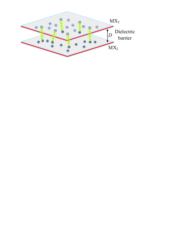
Figure 1: Spatially separated electrons and holes in two monolayers of TMDC.

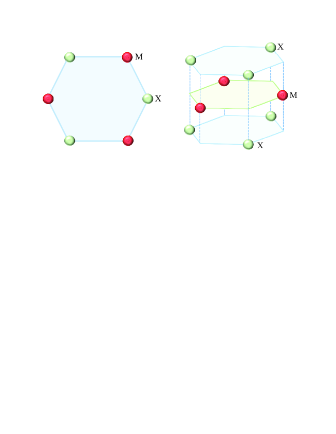
Figure 2: The structure of a TMDC monolayer.

We consider two parallel TMDC layers with the interlayer separation $D$. The dipolar excitons in this double-layer system are formed by the electrons located in one TMDC layer, while the holes located in another one. Let us mention that the electron moves in one TMDC layer, and the hole moves in the other TMDC layer. So the coordinate vectors of the electron and hole can be replaced by their 2D projections on plane of one of the TMDC layer. These new in-plane coordinates $\mathbf{r}_{1}$ and $\mathbf{r}_{2}$ for an electron and a hole, correspondingly, will be used everywhere below. In each TMDC layer a quasiparticle is characterized by the coordinates $\mathbf{r}_{j}$ in the conduction ($c$) and valence ($v$) band with the corresponding direction of spin ($s_{j})$ up $\uparrow$ or down $\downarrow$, and index $j=1,2$ referring to the two monolayers, one with electrons and the other with holes. The spinful basis for description of two particles in different monolayers is given by $\left\{\left|\Psi_{jc},s_{jc}\right\rangle,\left|\Psi_{jv},s_{jv}\right\rangle\right\}$, where $\left|\Psi_{jc},s_{jc}\right\rangle=\left|\Psi_{jc}\right\rangle\otimes\left|s_{jc}\right\rangle$ and $\left|\Psi_{jv},s_{jv}\right\rangle=\left|\Psi_{jv}\right\rangle\otimes\left|s_{jv}\right\rangle$ with the coordinate wave functions $\left|\Psi_{jc}\right\rangle$ and $\left|\Psi_{jv}\right\rangle$ and spin wave functions $\left|s_{jc}\right\rangle$ and $\left|s_{jv}\right\rangle,$ where $s=\left\{\uparrow,\downarrow\right\}$ is denoting the spin degree of freedom, in the conduction and valence bands for the first and second monolayers, correspondingly. Therefore, the two-particle wave function that describes the bound electron and hole in different monolayers, reads $\Psi_{s}(\mathbf{r}_{1},\mathbf{r}_{2})$. This wave function can also be understood as a four-component spinor, where the spinor components refer to the four possible values of the conduction/valence band indices:

$$\Psi_{\uparrow}(\mathbf{r}_{1},\mathbf{r}_{2})=\left({\begin{array}[]{c}\phi_{c\uparrow c\uparrow}(\mathbf{r}_{1},\mathbf{r}_{2})\\ \phi_{c\uparrow v\uparrow}(\mathbf{r}_{1},\mathbf{r}_{2})\\ \phi_{v\uparrow c\uparrow}(\mathbf{r}_{1},\mathbf{r}_{2})\\ \phi_{v\uparrow v\uparrow}(\mathbf{r}_{1},\mathbf{r}_{2})\end{array}}\right)\equiv\left({\begin{array}[]{c}\Psi_{c\uparrow}\\ \Psi_{v\uparrow}\end{array}}\right),\text{ where }\Psi_{c\uparrow}=\left({\begin{array}[]{c}\phi_{c\uparrow c\uparrow}\\ \phi_{c\uparrow v\uparrow}\end{array}}\right),\ \ \ \Psi_{v\uparrow}=\left({\begin{array}[]{c}\phi_{v\uparrow c\uparrow}\\ \phi_{v\uparrow v\uparrow}\end{array}}\right)\ .$$ (12)

The two components reflect one particle being in the conduction (valence) band and the other particle being in the valence (conduction) band, correspondingly. Let us mention that while Eq. (12) represents the spin-up particles, the spin-down particles are represented by the same expression replacing $\uparrow$ by $\downarrow$.

Each TMDC layer has an energy gap. Following the procedure applied for double-layer gapped graphene in Ref. BKZ, , the Hamiltonian $H_{\uparrow(\downarrow)}$ for spin-up (spin-down) particles can be written as

$$\mathcal{H}_{\uparrow(\downarrow)}=\left(\begin{array}[]{cccc}V(r)&d_{2}&d_{1}&0\\ d_{2}^{\dagger}&-\Delta^{\prime}+V(r)&0&d_{1}\\ d_{1}^{\dagger}&0&\Delta^{\prime}+V(r)&d_{2}\\ 0&d_{1}^{\dagger}&d_{2}^{\dagger}&V(r)\end{array}\right)\ ,$$ (17)

where $V(r)$ is the potential energy of the attraction between an electron and a hole, the parameter $\Delta^{\prime}$ is defined as $\Delta^{\prime}=\Delta-\lambda$ for spin-up particles, and $\Delta^{\prime}=\Delta+\lambda$ for spin-down particles. In Eq. (17) $d_{1}=at(-i\partial_{x_{1}}-\partial_{y_{1}})$, $d_{2}=at(-i\partial_{x_{2}}-\partial_{y_{2}})$ and the corresponding Hermitian conjugates are $d_{1}^{\dagger}=at(-i\partial_{x_{1}}+\partial_{y_{1}})$, $d_{2}^{\dagger}=at(-i\partial_{x_{2}}+\partial_{y_{2}})$, where $\partial_{x}=\partial/\partial x$ and $\partial_{y}=\partial/\partial y,$ $x_{1}$, $y_{1}$ and $x_{2}$, $y_{2}$ are the coordinates of vectors $\mathbf{r}_{1}$ and $\mathbf{r}_{2}$, correspondingly.

The single-particle energy spectrum of an electron-hole pair can be found by solving the eigenvalue problem for Hamiltonian (17):

$$\mathcal{H}_{\uparrow(\downarrow)}\Psi_{\uparrow(\downarrow)}=\epsilon_{\uparrow(\downarrow)}\Psi_{\uparrow(\downarrow)}\ ,$$ (18)

where $\Psi_{\uparrow(\downarrow)}$ are four-component eigenfunctions as given in Eq. (12), and $\epsilon_{\uparrow(\downarrow)}$ is the single-particle energy spectrum for an electron-hole pair with the up and down spin orientation, correspondingly. In this notation we assume that a spin-up (-down) hole describes the absence of a spin-down (-up) valence electron.

For Hamiltonian (17) the center-of-mass motion cannot be separated from the relative motion due the chiral nature of Dirac electron in TMDC. The similar conclusion was made for the two-particle problem in graphene in Ref. Sabio, and gapped graphene in Ref. BKZ, . Since the electron-hole Coulomb interaction depends only on the relative coordinate, we introduce the new “center-of-mass” coordinates in the plane of a TMDC layer:

$$\mathbf{R}=\alpha\mathbf{r}_{1}+\beta\mathbf{r}_{2}\ ,$$

$$\mathbf{r}=\mathbf{r}_{1}-\mathbf{r}_{2}\ ,$$ (19)

were the coefficients $\alpha$ and $\beta$ are supposed to be found below from the condition of the separation of the coordinates of the center-of-mass and relative motion in the Hamiltonian in the one-dimensional equation for the corresponding component of the wave function.

We make the following Anzätze to obtain the solution of Eq. (18)

$$\Psi_{j\uparrow(\downarrow)}(\mathbf{R},\mathbf{r})=\mathtt{e}^{i\mathbf{K}\cdot\mathbf{R}}\psi_{j\uparrow(\downarrow)}(\mathbf{r})\ ,$$ (20)

and follow the procedure described for the two-body problem in double-layer gapped graphene in Ref. BKZ, . The solution of a two-particle problem is demonstrated in Appendix A. Finally Eq. (101) that describes the bound electron-hole system can be written in the following form

$$\left(-F_{1}(\epsilon_{\uparrow(\downarrow)})\nabla_{\mathbf{r}}^{2}+V(r)\right)\phi_{c\uparrow(\downarrow)v\uparrow(\downarrow)}=F_{0}^{\prime}(\epsilon_{\uparrow(\downarrow)})\phi_{c\uparrow(\downarrow)v\uparrow(\downarrow)}\ ,$$ (21)

where

$$F_{1}(\epsilon_{\uparrow(\downarrow)})=\frac{2a^{2}t^{2}}{\epsilon_{\uparrow(\downarrow)}}\ ,\hskip 142.26378ptF_{0}^{\prime}(\epsilon_{\uparrow(\downarrow)})=\epsilon_{\uparrow(\downarrow)}+\Delta^{\prime}-\frac{a^{2}t^{2}\mathcal{K}^{2}}{2\epsilon_{\uparrow(\downarrow)}}\ .$$ (22)

We consider spatially separated an electron and a hole in two parallel TMDC layers at large distances $D\gg a_{B}$, where $a_{B}$ is a 2D Bohr radius of a dipolar exciton. For TMDC materials the Bohr radius of the dipolar exciton is found to be in the rangde from $1.5\ \mathrm{{\mathring{A}}}$ for $\mathrm{MoTe_{2}}$ Ashwin up to $3.9\ \mathrm{{\mathring{A}}}$ for $\mathrm{MoS_{2}}$ Louie .

It is obvious that the electron and hole are interacting via the Coulomb potential. However, in general, the electron-hole interaction is effected by the screening effects Reichman . However, the screening effects are negligible at long range for electron-hole distances larger than the screening length $\rho_{0}$, and at long range the electron-hole interaction is described by the Coulomb’s potential Reichman . The screening length is defined as $\rho_{0}=2\pi\chi_{2D}$, where $\chi_{2D}$ is the 2D polarizability of the planar material Rubio . Substituting $\chi_{2D}$ from Ref. Reichman, , we conclude that for TMDC $\rho_{0}$ is estimated as $38\ \mathrm{{\mathring{A}}}$ for $\mathrm{WS_{2}}$, $41\ \mathrm{{\mathring{A}}}$ for $\mathrm{MoS_{2}}$, $45\ \mathrm{{\mathring{A}}}$ for $\mathrm{WSe_{2}}$, $52\ \mathrm{{\mathring{A}}}$ for $\mathrm{MoSe_{2}}$. The binding energy for the dipolar exciton was estimated for two $\mathrm{MoS_{2}}$ layers separated by $N$ hBN insulating layers from $N=1$ up to $N=6$ Fogler . These dipolar excitons were observed experimentally for $N=2$ Calman . The interlayer separation $D$ is given by $D=Nc$, where $c=0.333\ \mathrm{nm}$ Fogler . We assume that the indirect excitons in TMDC can survive for a larger interlayer separation $D$ than in semiconductor coupled quantum wells, because the thickness of a TMDC layer is fixed (for example, for $\mathrm{MoS_{2}}$ this thickness is $0.312\ \mathrm{nm}$ Fogler ), while the spatial fluctuations of the thickness of the semiconductor quantum well effect the structure of the dipolar exciton.

Since for the TMDCs materials the characteristic values for the 2D exciton Bohr radius are found to be much less than the characteristic values of the screening length $\rho_{0}$, Coulomb’s potential describes the electron hole interaction for $D>\rho_{0}$. Otherwise, for $D\lesssim\rho_{0}$, the electron-hole interaction is described by Keldysh’s potential due to the screening effects Keldysh . Though the two-body electron-hole problem with Keldysh’s potential can be solved only numerically, it cannot be solved analytically. We solve the two-body electron-hole problem analytically for large interlayer distances $D>\rho_{0}$. In this case, when the screening effects for the interaction between an electron and a hole at large distances are negligible, the potential energy $V(r)$ corresponding to the attraction between an electron and a hole is given by

$$V(r)=-\frac{ke^{2}}{\epsilon_{d}\sqrt{r^{2}+D^{2}}}\ ,$$ (23)

where $k=9\times 10^{9}\ N\times m^{2}/C^{2}$, $\epsilon_{d}$ is the dielectric constant of the dielectric, which separates two TMDC layers. Assuming $r\ll D$, we approximate $V(r)$ by the first two terms of the Taylor series, and substituting

$$V(r)=-V_{0}+\gamma r^{2}\ ,$$ (24)

where

$$V_{0}=\frac{ke^{2}}{\epsilon_{d}D}\ ,\hskip 142.26378pt\gamma=\frac{ke^{2}}{2\epsilon_{d}D^{3}}\ ,$$ (25)

into Eq. (21), one obtains the equation in the form of Schrödinger equation for the 2D isotropic harmonic oscillator:

$$\left(-F_{1}(\epsilon_{\uparrow(\downarrow)})\nabla_{\mathbf{r}}^{2}+\gamma r^{2}\right)\phi_{c\uparrow(\downarrow)v\uparrow(\downarrow)}=F_{0}(\epsilon_{\uparrow(\downarrow)})\phi_{c\uparrow(\downarrow)v\uparrow(\downarrow)}\ ,$$ (26)

where

$$F_{0}(\epsilon_{\uparrow(\downarrow)})=\epsilon_{\uparrow(\downarrow)}+\Delta^{\prime}+V_{0}-\frac{a^{2}t^{2}\mathcal{K}^{2}}{2\epsilon_{\uparrow(\downarrow)}}\ .$$ (27)

The solution of the Schrödinger equation for the harmonic oscillator, is well known and is given by

$$\frac{\mathcal{F}_{0}(\epsilon_{\uparrow(\downarrow)})}{\mathcal{F}_{1}(\epsilon_{\uparrow(\downarrow)})}=2N\sqrt{\frac{\gamma}{\mathcal{F}_{1}(\epsilon_{\uparrow(\downarrow)})}}\ ,$$ (28)

where $N=2\tilde{N}+|L|+1$, and $\tilde{N}=\mathrm{min}(\widetilde{n},\widetilde{n}^{\prime})$, $L=\widetilde{n}-\widetilde{n}^{\prime}$, $\widetilde{n},$ $\widetilde{n}^{\prime}=0,1,2,3,\ldots$ are the quantum numbers of the 2D harmonic oscillator. The corresponding 2D wave function at $\mathcal{K}=0$ in terms of associated Laguerre polynomials can be written as

$$\phi_{c\uparrow(\downarrow)v\uparrow(\downarrow)\tilde{N}\text{ }L,\mathcal{K}=0}(r)=\frac{\tilde{N}!}{a_{B}^{|L|+1}\sqrt{\widetilde{n}!\widetilde{n}^{\prime}!}}\mathrm{sgn}(L)^{L}r^{|L|-1/2}e^{-r^{2}/(4a_{B}^{2})}\times L_{\tilde{N}}^{|L|}(r^{2}/(2a_{B}^{2}))\frac{e^{-iL\phi}}{(2\pi)^{1/2}}\ ,$$ (29)

where $\phi$ is the polar angle, $L_{k}^{p}(x)$ are the associated Laguerre polynomials. and the Bohr radius of the dipolar exciton $a_{B}$ is given by

$$a_{B}=\left(\sqrt{F_{1}(\epsilon)}/\left(2\sqrt{\gamma}\right)\right)^{1/2}=\left(\frac{at}{\sqrt{2\gamma\left|\epsilon\right|}}\right)^{1/2}\ .$$ (30)

Substituting Eqs. (22) and (27) into Eq. (28), we obtain

$$2\epsilon_{\uparrow(\downarrow)}^{2}+2\left(\Delta^{\prime}+V_{0}\right)\epsilon_{\uparrow(\downarrow)}-\frac{8atN\sqrt{\gamma\epsilon_{\uparrow(\downarrow)}}}{\sqrt{2}}-a^{2}t^{2}\mathcal{K}^{2}=0\ .$$ (31)

The solution of Eq. (31) for the single exciton spectrum is shown in Appendix B. From Eq. (109), for the single exciton spectrum one obtains

$$\epsilon_{A(B)}=x_{0}^{2}+\frac{\hbar^{2}\mathcal{K}^{2}}{2M_{A(B)}}\ ,$$ (32)

where $M_{A(B)}$ is the dipolar exciton effective mass given by

$$M_{A(B)}=\frac{C_{A(B)}\hbar^{2}}{2a^{2}t^{2}x_{0}}\ ,$$ (33)

where in Eqs. (32) and (33) $x_{0}$ has the different value for A and B excitons.

The dipolar exciton binding energy is given by

$$E_{b\ A(B)}=-\left(x_{0}^{2}-\Delta^{\prime}\right)\ .$$ (34)

In Eq. (34), we assume $\Delta^{\prime}=\Delta-\lambda$ for A excitons, and $\Delta^{\prime}=\Delta+\lambda$ for B excitons.

III The collective excitations for spatially separated electrons and holes

Let us consider the dilute limit for the electrons and holes gases in parallel TMDC layers spatially separated by the dielectric, when $n_{A}a_{B\ A}^{2}\ll 1$ and $n_{B}a_{B\ B}^{2}\ll 1$, where $n_{A(B)}$ and $a_{B\ A(B)}$ are the concentration and effective exciton Bohr radius for A(B) dipolar excitons, correspondingly. In the experiments, the exciton density in a $\mathrm{WSe_{2}}$ monolayer was obtained up to $n=5\times 10^{11}\ \mathrm{cm^{-2}}$ You_bi . In the dilute limit, the dipolar A and B excitons are formed by the electron-hole pairs with the electrons and holes spatially separated in two different TMDC layers. The Hamiltonian $\hat{H}$ of the 2D A and B interacting dipolar excitons is given by

$$\hat{H}=\hat{H}_{A}+\hat{H}_{B}+\hat{H}_{I}\ ,$$ (35)

where $\hat{H}_{A(B)}$ are the Hamiltonians of A(B) excitons given by

$$\hat{H}_{A(B)}=\sum_{\mathbf{k}}E_{A(B)}(k)a_{\mathbf{k}A(B)}^{\dagger}a_{\mathbf{k}A(B)}+\frac{g_{AA(BB)}}{2S}\sum_{\mathbf{k}\mathbf{l}\mathbf{m}}a_{\mathbf{k}A(B)}^{\dagger}a_{\mathbf{l}A(B)}^{\dagger}a_{A(B)\mathbf{m}}a_{A(B)\mathbf{k}+\mathbf{l}-\mathbf{m}}\ ,$$ (36)

and $\hat{H}_{I}$ is the Hamiltonian of the interaction between A and B excitons given by

$$\hat{H}_{I}=\frac{g_{AB}}{S}\sum_{\mathbf{k}\mathbf{l}\mathbf{m}}a_{\mathbf{k}A}^{\dagger}a_{\mathbf{l}B}^{\dagger}a_{B\mathbf{m}}a_{A\mathbf{k}+\mathbf{l}-\mathbf{m}}\ ,$$ (37)

where $a_{\mathbf{k}A(B)}^{\dagger}$ and $a_{\mathbf{k}A(B)}$ are Bose creation and annihilation operators for A(B) dipolar excitons with the wave vector $\mathbf{k}$, correspondingly, $S$ is the area of the system, $E_{A(B)}(k)\equiv\epsilon_{A(B)}=\varepsilon_{(0)A(B)}(k)+\mathcal{A}_{A(B)}$ is the energy spectrum of non-interacting A(B) dipolar excitons, correspondingly, $\varepsilon_{(0)A(B)}(k)=\hbar^{2}k^{2}/(2M_{A(B)})$, $M_{A(B)}$ is an effective mass of non-interacting dipolar excitons, $\mathcal{A}_{A(B)}$ is the constant, which depends on A(B) dipolar exciton binding energy and the gap, formed by a spin-orbit coupling for the A(B) dipolar exciton, $g_{AA(BB)}$ and $g_{AB}$ are the interaction constants for the interaction between two A dipolar excitons, two B dipolar excitons with the same conduction band electron spin orientation and for the interaction between A and B dipolar excitons with the opposite conduction band electron spin orientation.

We consider the dilute system, when the average distance between the excitons is much larger than the interlayer separation $D$, which corresponds to the densities $n\ll 1/(\pi D^{2})$. Since we assume that $D>\rho_{0}$, the screening effects are negligible, and the interaction between the particles is described by the Coulomb’s potential. For example, for $D=50\ \mathrm{{\mathring{A}}}$, the exciton densities should be $n\ll 1.3\times 10^{12}\ \mathrm{cm^{-2}}$.

In the dilute system at the large interlayer separation $D$, two dipolar excitons at the distance $R$ repel due to the dipole-dipole interaction potential $U(R)=ke^{2}D^{2}/(\epsilon_{d}R^{3})$. Following the procedure presented in Ref. BKKL, , the interaction parameters for the exciton-exciton interaction in very dilute systems could be obtained assuming the exciton-exciton dipole-dipole repulsion exists only at the distances between excitons greater than distance from the exciton to the classical turning point. The distance between two excitons cannot be less than this distance, which is determined by the conditions reflecting the fact that the energy of two excitons cannot exceed doubled chemical potential of the system $\mu$:

$$2\mathcal{A}_{A}+U(R_{0AA})=2\mu\ ,\hskip 42.67912pt2\mathcal{A}_{B}+U(R_{0BB})=2\mu\ ,\hskip 42.67912pt\mathcal{A}_{A}+\mathcal{A}_{B}+U(R_{0AB})=2\mu\ ,$$ (38)

where $R_{0AA}$, $R_{0BB}$, and $R_{0AB}$ are distances between two dipolar excitons at the classical turning point for two A excitons, two B excitons, and one A and one B excitons, correspondingly. Let us mention that in the thermodynamical equilibrium the chemical potentials of A and B dipolar excitons are equal.

From Eq. (38) the following expressions are obtained

$$R_{0AA}=\left(\frac{ke^{2}D^{2}}{2\epsilon_{d}\left(\mu-\mathcal{A}_{A}\right)}\right)^{1/3}\ ,\hskip 28.45274ptR_{0BB}=\left(\frac{ke^{2}D^{2}}{2\epsilon_{d}\left(\mu-\mathcal{A}_{B}\right)}\right)^{1/3}\ ,\hskip 28.45274ptR_{0AB}=\left(\frac{ke^{2}D^{2}}{\epsilon_{d}\left(2\mu-\mathcal{A}_{A}-\mathcal{A}_{B}\right)}\right)^{1/3}\ .$$ (39)

Following the procedure presented in Ref. BKKL, , one can obtain the interaction constants for the exciton-exciton interaction

$$g_{AA}=\frac{2\pi ke^{2}D^{2}}{\epsilon_{d}R_{0AA}}\ ,\hskip 85.35826ptg_{BB}=\frac{2\pi ke^{2}D^{2}}{\epsilon_{d}R_{0BB}}\ ,\hskip 85.35826ptg_{AB}=\frac{2\pi ke^{2}D^{2}}{\epsilon_{d}R_{0AB}}\ .$$ (40)

We expect that at zero temperature $T=0$ almost all A and B excitons belong to the BEC of A and B excitons, correspondingly. Therefore, we assume the formation of the binary mixture of BECs. Using Bogoliubov approximation Lifshitz , generalized for two-component weakly-interacting Bose gas Timmermans , we obtain the chemical potential $\mu$ of the entire exciton system by minimizing $\hat{H}_{0}-\mu\hat{N}$ with respect to 2D concentration $n$, where $\hat{N}$ denotes the number operator

$$\hat{N}=\sum_{\mathbf{k}}a_{\mathbf{k}A}^{\dagger}a_{\mathbf{k}A}+\sum_{\mathbf{k}}a_{\mathbf{k}B}^{\dagger}a_{\mathbf{k}B}\ ,$$ (41)

and $H_{0}$ is the Hamiltonian describing the particles in the condensate with zero momentum $\mathbf{k}=0$. In the Bologoiubov approximation we assume $N=N_{0}$, $a_{\mathbf{k}=0,A(B)}^{\dagger}=\sqrt{N_{0A(B)}}e^{-i\Theta_{A(B)}}$ and $a_{\mathbf{k}=0,A(B)}=\sqrt{N_{0A(B)}}e^{i\Theta_{A(B)}}$, where $N$ is the total number of all excitons, and $N_{0}$ is the number of all excitons in the condensate, $N_{0A(B)}$ and $\Theta_{A(B)}$ are the number and phase for A(B) excitons in the corresponding condensate. From Eqs. (35), (36), and (37) we obtain

$$\hat{H}_{0}-\mu\hat{N}=S\left[\left(\mathcal{A}_{A}-\mu\right)n_{A}+\left(\mathcal{A}_{B}-\mu\right)n_{B}+\frac{g_{AA}n_{A}^{2}}{2}+\frac{g_{BB}n_{B}^{2}}{2}+g_{AB}n_{A}n_{B}\right]\ ,$$ (42)

where $n_{A}$ and $n_{B}$ are the 2D concentrations of A and B excitons, correspondingly. The minimization of $\hat{H}_{0}-\mu\hat{N}$ with respect to the number of A excitons $N_{A}=Sn_{A}$ results in

$$\mu-\mathcal{A}_{A}=g_{AA}n_{A}+g_{AB}n_{B}\ .$$ (43)

The minimization of $\hat{H}_{0}-\mu\hat{N}$ with respect to the number of B excitons $N_{B}=Sn_{B}$ results in

$$\mu-\mathcal{A}_{B}=g_{BB}n_{B}+g_{AB}n_{A}\ .$$ (44)

From Eqs. (43) and (44), we obtain

$$2\mu-\mathcal{A}_{A}-\mathcal{A}_{B}=g_{AA}n_{A}+g_{BB}n_{B}+g_{AB}n\ ,$$ (45)

where $n=n_{A}+n_{B}$ is the total 2D concentration of excitons.

Combining Eqs. (39), (40), (43), (44), (45), one obtains the following system of three cubical equations for the interaction constants $g_{AA}$, $g_{BB}$, $g_{AB}$:

$$g_{AA}^{3}-2\mathcal{B}n_{A}g_{AA}-2\mathcal{B}n_{B}g_{AB}=0\ ,$$

$$g_{BB}^{3}-2\mathcal{B}n_{B}g_{BB}-2\mathcal{B}n_{A}g_{AB}=0\ ,$$ (46)

$$g_{AB}^{3}-\mathcal{B}ng_{AB}-\mathcal{B}\left(n_{A}g_{AA}+n_{B}g_{BB}\right)=0\ ,$$

where $B$ are defined as

$$\mathcal{B}=\frac{(2\pi)^{3}(ke^{2}D^{2})^{2}}{\epsilon_{d}^{2}}\ .$$ (47)

Making the sum of the top two equations in (III), we can replace Eq. (III) by the following system of three cubical equations:

$$g_{AA}^{3}-2\mathcal{B}n_{A}g_{AA}-2\mathcal{B}n_{B}g_{AB}=0\ ,$$

$$g_{BB}^{3}-2\mathcal{B}n_{B}g_{BB}-2\mathcal{B}n_{A}g_{AB}=0\ ,$$ (48)

$$2g_{AB}^{3}=g_{AA}^{3}+g_{BB}^{3}\ .$$

The interaction constants $g_{AA}$, $g_{BB}$, $g_{AB}$ can be obtained from the solution of the system of three cubical equations represented by Eq. (III).

If the interaction constants for exciton-exciton interaction are negative, the spectrum of collective excitations at small momenta is imaginary which reflects the instability of the excitonic ground state BKL_i ; BKL_ii . The system of equations Eq. (III) has all real and positive roots only if $g_{AA}=g_{BB}=g_{AB}\equiv g$. Substituting this condition into Eq. (III), we obtain

$$g^{3}-2\mathcal{B}\left(n_{A}+n_{B}\right)g=0\ .$$ (49)

Using $n=n_{A}+n_{B}$, we get from Eq. (49) the following expression for $g$

$$g=\sqrt{2\mathcal{B}n}\ .$$ (50)

Substituting $\mathcal{B}$ from Eq. (47) into Eq. (50), we obtain $g$ as

$$g=\frac{4\pi ke^{2}D^{2}\sqrt{\pi n}}{\epsilon_{d}}\ .$$ (51)

Using the following notation,

$$G_{AA} = g_{AA}n_{A}=gn_{A},\hskip 56.9055ptG_{BB}=g_{BB}n_{B}=gn_{B},\hskip 56.9055ptG_{AB}=g_{AB}\sqrt{n_{A}n_{B}}=g\sqrt{n_{A}n_{B}}\ ,$$

$$\omega_{A}(k) = \sqrt{\varepsilon_{(0)A}^{2}(k)+2G_{AA}\varepsilon_{(0)A}(k)}\ ,$$ (52)

$$\omega_{B}(k) = \sqrt{\varepsilon_{(0)B}^{2}(k)+2G_{BB}\varepsilon_{(0)B}(k)}\ ,$$

we obtain two modes of the spectrum of Bose collective excitations $\varepsilon_{j}(k)$ in the Bogoliubov approximation for two-component weakly-interacting Bose gas Sun

$$\varepsilon_{j}(k)=\sqrt{\frac{\omega_{A}^{2}(k)+\omega_{B}^{2}(k)+(-1)^{j-1}\sqrt{\left(\omega_{A}^{2}(k)-\omega_{B}^{2}(k)\right)^{2}+\left(4G_{AB}\right)^{2}\varepsilon_{(0)A}(k)\varepsilon_{(0)B}(k)}}{2}}\ ,$$ (53)

where $j=1$, $2$. We can note that $G_{AB}^{2}=G_{AA}G_{BB}$.

In the limit of small momenta $p$, when $\varepsilon_{(0)A}(k)\ll G_{AA}$ and $\varepsilon_{(0)B}(k)\ll G_{BB}$, we expand the spectrum of collective excitations $\varepsilon_{j}(k)$ up to the first order with respect to the momentum $p=\hbar k$ and get two sound modes of the collective excitations $\varepsilon_{j}(p)=c_{j}p$, where $c_{j}$ is the sound velocity given by

$$c_{j}=\sqrt{\frac{G_{AA}}{2M_{A}}+\frac{G_{BB}}{2M_{B}}+(-1)^{j-1}\sqrt{\left(\frac{G_{AA}}{2M_{A}}-\frac{G_{BB}}{2M_{B}}\right)^{2}+\frac{G_{AB}^{2}}{M_{A}M_{B}}}}\ ,$$ (54)

In the limit of large momenta, when $\varepsilon_{(0)A}(k)\gg G_{AA}$ and $\varepsilon_{(0)B}(k)\gg G_{BB}$, we get two parabolic modes of collective excitations with the spectra $\varepsilon_{1}(k)=\varepsilon_{(0)A}(k)$ and $\varepsilon_{2}(k)=\varepsilon_{(0)B}(k)$, if $M_{A}<M_{B}$ and if $M_{A}>M_{B}$ with the spectra $\varepsilon_{1}(k)=\varepsilon_{(0)B}(k)$ and $\varepsilon_{2}(k)=\varepsilon_{(0)A}(k)$ .

The Hamiltonian $\hat{H}_{col}$ of the collective excitations, corresponding to two branches of the spectrum, in the Bogoliubov approximation for the entire two-component system is given by Sun

$$\hat{H}_{col}=\sum_{\mathbf{k}\neq 0}\varepsilon_{1}(k)\alpha_{1\mathbf{k}}^{\dagger}\alpha_{1\mathbf{k}}+\sum_{\mathbf{k}\neq 0}\varepsilon_{2}(k)\alpha_{2\mathbf{k}}^{\dagger}\alpha_{2\mathbf{k}}\ ,$$ (55)

where $\alpha_{j\mathbf{k}}^{\dagger}$ and $\alpha_{j\mathbf{k}}$ are the creation and annihilation Bose operators for the quasiparticles with the energy dispersion corresponding to the $j$th mode of the spectrum of the collective excitations.

If A and B excitons do not interact, we put $g_{AB}=0$ and $G_{AB}=0$, and in the limit of the small momenta we get for the sound velocity $c_{1}=\sqrt{\frac{G_{AA}}{M_{A}}}$ and $c_{2}=\sqrt{\frac{G_{BB}}{M_{B}}}$, which satisfies to the sound velocity in the Bogoliubov approximation for one-component system Lifshitz .

If for simplicity we consider the specific case when the densities of A and B excitons are the same $n_{A}=n_{B}=n/2$, we get from Eq. (III)

$$G_{AA} = G_{BB}=G_{AB}=gn/2\ ,$$

$$\omega_{A}(k) = \sqrt{\varepsilon_{(0)A}^{2}(k)+gn\varepsilon_{(0)A}(k)}\ ,$$ (56)

$$\omega_{B}(k) = \sqrt{\varepsilon_{(0)B}^{2}(k)+gn\varepsilon_{(0)B}(k)}\ .$$

From Eq. (53), we get the spectrum of collective excitations

$$\varepsilon_{j}(k)=\sqrt{\frac{\omega_{A}^{2}(k)+\omega_{B}^{2}(k)+(-1)^{j-1}\sqrt{\left(\omega_{A}^{2}(k)-\omega_{B}^{2}(k)\right)^{2}+4g^{2}n^{2}\varepsilon_{(0)A}(k)\varepsilon_{(0)B}(k)}}{2}}\ ,$$ (57)

and the sound velocity at $n_{A}=n_{B}=n/2$ is obtained as

$$c_{j}=\sqrt{\frac{gn}{2}\left(\frac{1}{2M_{A}}+\frac{1}{2M_{B}}+(-1)^{j-1}\sqrt{\left(\frac{1}{2M_{A}}-\frac{1}{2M_{B}}\right)^{2}+\frac{1}{M_{A}M_{B}}}\right)}\ .$$ (58)

It follows from Eq. (58), that there is only one non-zero sound velocity at $n_{A}=n_{B}=n/2$ given by

$$c=\sqrt{\frac{gn}{2}\left(\frac{1}{M_{A}}+\frac{1}{M_{B}}\right)}\ .$$ (59)

Interestingly enough, if for an one-component system the sound velocity is inversely proportional to the square root of the mass of the exciton, $M_{A}^{-1/2}$, $M_{B}^{-1/2}$ one or the other, for a two-component system it is inversely proportional to the square root of the reduced mass of two excitons, $\mu_{AB}^{-1/2}$, where $\mu_{AB}=M_{A}M_{B}/(M_{A}+M_{B})$. Since $M_{A}>\mu_{AB}$ and $M_{B}>\mu_{AB}$, it is always true that $M_{A}^{-1/2}<\mu_{AB}^{-1/2}$ or $M_{B}^{-1/2}<\mu_{AB}^{-1/2}.$ Thus, in the Bogoliubov approximation the sound velocity in a two-component system is always larger than in an one-component system.

IV Superfluidity

Since at small momenta the energy spectrum of the quasiparticles in the weakly-interacting gas of dipolar excitons is soundlike, this system satisfies to the Landau criterion for superfluidity Lifshitz ; Abrikosov . The critical velocity for the superfluidity is given by $v_{c}=\min\left(c_{1},c_{2}\right)$, because the quasiparticles are created at the velocities above the velocity of sound for the lowest mode of the quasiparticle dispersion.

The density of the superfluid component $\rho_{s}(T)$ is defined as $\rho_{s}(T)=\rho-\rho_{n}(T)$, where $\rho=M_{A}n_{A}+M_{B}n_{B}$ is the total 2D density of the system and $\rho_{n}(T)$ is the density of the normal component. We define the normal component density $\rho_{n}(T)$ by the standard procedure Pitaevskii . Suppose that the exciton system moves with a velocity $\mathbf{u}$, which means that the superfluid component moves with the velocity $\mathbf{u}$. At nonzero temperatures $T$ dissipating quasiparticles will appear in this system. Since their density is small at low temperatures, one can assume that the gas of quasiparticles is an ideal Bose gas. To calculate the superfluid component density, we define the total mass current for a two-component Bose-gas of quasiparticles in the frame, in which the superfluid component is at rest, as

$$\mathbf{J}=\int\frac{d^{2}p}{(2\pi\hbar)^{2}}\mathbf{p}\left(f\left[\varepsilon_{1}(p)-\mathbf{p}\mathbf{u}\right]+f\left[\varepsilon_{2}(p)-\mathbf{p}\mathbf{u}\right]\right)\ ,$$ (60)

where $f\left[\varepsilon_{1}(p))\right]=\left(\exp\left[\varepsilon_{1}(p)/(k_{B}T)\right]-1\right)^{-1}$ and $f\left[\varepsilon_{2}(p))\right]=\left(\exp\left[\varepsilon_{2}(p)/(k_{B}T)\right]-1\right)^{-1}$ are the Bose-Einstein distribution function for the quasiparticles with the dispersion $\varepsilon_{1}(p)$ and $\varepsilon_{2}(p)$, correspondingly, $k_{B}$ is the Boltzmann constant. Expanding the expression under the integral in terms of $\mathbf{p}\mathbf{u}/(k_{B}T)$ and restricting ourselves by the first order term, we obtain:

$$\mathbf{J}=-\frac{\mathbf{u}}{2}\int\frac{d^{2}p}{(2\pi\hbar)^{2}}p^{2}\left(\frac{\partial f\left[\varepsilon_{1}(p)\right]}{\partial\varepsilon_{1}(p)}+\frac{\partial f\left[\varepsilon_{2}(p)\right]}{\partial\varepsilon_{2}(p)}\right)\ .$$ (61)

The density $\rho_{n}$ of the normal component is defined as Pitaevskii

$$\mathbf{J}=\rho_{n}\mathbf{u}\ .$$ (62)

Using Eqs. (61) and (62), we obtain the density of the normal component as

$$\rho_{n}(T)=-\frac{1}{2}\int\frac{d^{2}p}{(2\pi\hbar)^{2}}p^{2}\left(\frac{\partial f\left[\varepsilon_{1}(p)\right]}{\partial\varepsilon_{1}(p)}+\frac{\partial f\left[\varepsilon_{2}(p)\right]}{\partial\varepsilon_{2}(p)}\right)\ .$$ (63)

At small temperatures $k_{B}T\ll M_{A(B)}c_{j}^{2}$, the small momenta, corresponding to the conditions $\varepsilon_{(0)A}(k)\ll G_{AA}$ and $\varepsilon_{(0)B}(k)\ll G_{BB}$ provide the main contribution to the integral in the r.h.s. of Eq. (63), which corresponds to the quasiparticles with the sound spectrum $\varepsilon_{j}(k)=c_{j}k$ with the sound velocity given by Eq. (54), results in

$$\rho_{n}(T)=\frac{3\zeta(3)}{2\pi\hbar^{2}}k_{B}^{3}T^{3}\left(\frac{1}{c_{1}^{4}}+\frac{1}{c_{2}^{4}}\right)\ ,$$ (64)

where $\zeta(z)$ is the Riemann zeta function ($\zeta(3)\simeq 1.202$).

For high temperatures $k_{B}T\gg M_{A(B)}c_{j}^{2}$, the large momenta $M_{A(B)}c_{j}^{2}\ll\varepsilon_{0A(B)}(k)\ll k_{B}T$ provide the main contribution to the integral in the r.h.s. of Eq. (63), which corresponds to quasiparticles with the parabolic spectrum. Using the result for these values of momenta for one-component system Pitaevskii , we get for high temperatures

$$\rho_{n}(T)=\left\{\begin{array}[]{c}\frac{k_{B}T}{2\pi\hbar^{2}}\left(M_{A}^{2}\ln\frac{k_{B}T}{M_{A}c_{1}^{2}}+M_{B}^{2}\ln\frac{k_{B}T}{M_{B}c_{2}^{2}}\right)\ ,\text{ if }M_{A}<M_{B}\\ \frac{k_{B}T}{2\pi\hbar^{2}}\left(M_{A}^{2}\ln\frac{k_{B}T}{M_{A}c_{2}^{2}}+M_{B}^{2}\ln\frac{k_{B}T}{M_{B}c_{1}^{2}}\right)\ ,\text{ if }M_{A}>M_{B}\ .\end{array}\right.$$ (67)

Neglecting the interaction between the quasiparticles, the mean field critical temperature $T_{c}$ of the phase transition related to the occurrence of superfluidity is given by the condition $\rho_{s}(T_{c})=0$ Pitaevskii :

$$\rho_{n}(T_{c})=\rho=M_{A}n_{A}+M_{B}n_{B}\ .$$ (68)

At small temperatures $k_{B}T\ll M_{A(B)}c_{j}^{2}$ substituting Eq. (64) into Eq. (68), we get

$$T_{c}=\left[\frac{2\pi\hbar^{2}\rho}{3\zeta(3)k_{B}^{3}\left(\frac{1}{c_{1}^{4}}+\frac{1}{c_{2}^{4}}\right)}\right]^{1/3}\ .$$ (69)

If $T_{c}$ obtained from Eq. (69) satisfies to the condition $k_{B}T_{c}\ll M_{A(B)}c_{j}^{2}$, it is the right value of the mean field critical temperature. Otherwise, at high temperatures $k_{B}T\gg M_{A(B)}c_{j}^{2}$, we obtain the critical temperature $T_{c}$ from the solution of the equation

$$\rho=\left\{\begin{array}[]{c}\frac{k_{B}T_{c}}{2\pi\hbar^{2}}\left(M_{A}^{2}\ln\frac{k_{B}T_{c}}{M_{A}c_{1}^{2}}+M_{B}^{2}\ln\frac{k_{B}T_{c}}{M_{B}c_{2}^{2}}\right)\ ,\text{ if }M_{A}<M_{B}\\ \frac{k_{B}T_{c}}{2\pi\hbar^{2}}\left(M_{A}^{2}\ln\frac{k_{B}T_{c}}{M_{A}c_{2}^{2}}+M_{B}^{2}\ln\frac{k_{B}T_{c}}{M_{B}c_{1}^{2}}\right)\ ,\text{ if }M_{A}>M_{B}c\ .\end{array}\right.$$ (72)

At $n_{A}=n_{B}=n/2$, we get the density of the normal component as

$$\rho_{n}(T)=\left\{\begin{array}[]{c}\frac{3\zeta(3)k_{B}^{3}T^{3}}{2\pi\hbar^{2}c^{4}}\ ,\text{ at low temperatures }\\ \frac{k_{B}T}{2\pi\hbar^{2}}\left(M_{A}^{2}\ln\frac{k_{B}T}{M_{A}c^{2}}+M_{B}^{2}\ln\frac{k_{B}T}{M_{B}c^{2}}\right)\ ,\text{ at high temperatures. }\end{array}\right.$$ (75)

At $n_{A}=n_{B}=n/2$, for the low-temperature case we get the mean field critical temperature as

$$T_{c}=\left[\frac{2\pi\hbar^{2}\rho c^{4}}{3\zeta(3)k_{B}^{3}}\right]^{1/3}\ .$$ (76)

At the first glance, Eq.  (77) is the same as for one-component exciton gas. However, after consideration of (45), one obtains

$$T_{c}=\left[\frac{\pi\hbar^{2}g^{2}n^{3}}{12\zeta(3)}Q\right]^{1/3}\ .$$ (77)

where the parameter $Q$ is defined as

$$Q=\frac{M_{A}+M_{B}}{\left(\mu_{AB}\right)^{2}}\ ,$$ (78)

and $\mu_{AB}$ is the reduced mass for two-component system of A and B excitons. For one-component dilute exciton gas $Q_{A}=1/M_{A}$ or $Q_{B}=1/M_{B},$ that is always less than the value of $Q$ for a two-component Bose gas of A and B dipolar excitons. Therefore, $T_{c}$ is always higher for a two-component dilute dipolar exciton gas than for an one-component dilute dipolar exciton gas.

If $T_{c}$ obtained from Eq. (77) satisfies to the condition $k_{B}T_{c}\ll M_{A(B)}c^{2}$, it is the right value of the mean field critical temperature. Otherwise, at high temperatures $k_{B}T\gg M_{A(B)}c^{2}$, we obtain the critical temperature $T_{c}$ from the solution of the equation

$$\rho=\frac{k_{B}T_{c}}{2\pi\hbar^{2}}\left(M_{A}^{2}\ln\frac{k_{B}T_{c}}{M_{A}c^{2}}+M_{B}^{2}\ln\frac{k_{B}T_{c}}{M_{B}c^{2}}\right)\ ,$$ (79)

where $\rho=\left(M_{A}+M_{B}\right)n/2$.

V Two-component direct exciton superfluidity in a TMDC monolayer

Let us consider the two-component weakly interacting Bose gas of direct A and B excitons in a single TMDC monolayer. The direct excitons of type A are formed by spin-up electrons from conduction and spin-down holes from valence bands in a single TMDC monolayer.

There are two differences between two-component weakly interacting Bose gas of A and B excitons in a single TMDC monolayer and two parallel TMDC layers with the spatially separated charge carriers. The first difference is that the effective mass of direct excitons in a single TMDC monolayer is different from the effective mass of indirect excitons in two parallel TMDC layers given by Eq. (33). The second difference is that the interaction constant for the contact exciton-exciton repulsion for direct excitons in a single TMDC monolayer is different from the interaction constant for the dipole-dipole exciton-exciton repulsion for dipolar excitons in two parallel TMDC layers given by Eq. (51).

As discussed in Refs. Ciuti-exex, and Laikht, for a dilute exciton gas, the excitons can be treated as bosons with a repulsive contact interaction. For small wave vectors $q\ll\rho^{-1}$ the exciton-exciton interaction constant, describing the pairwise exciton-exciton repulsion between A and A (B and B) direct excitons, correspondingly, can be approximated by a contact potential

$$g_{AA(BB)}=\frac{6ke^{2}a_{A(B)}}{\varepsilon_{m}}\ ,$$ (80)

where $a_{A(B)}$ is the exciton Bohr radius for A(B) direct excitons, correspondingly. This direct exciton Bohr radius $a_{A(B)}$ can be obtained analagousely to $\tilde{\beta}$ in Eq. (39) in Ref. BKZ, for a gapped graphene monolayer. In Eq. (80), $\varepsilon_{m}$ is the dielectric constant for the media, surrounding the TMDC monolayer, and for a freely suspended TMDC material in vacuum we have $\varepsilon_{m}=1$. This approximation for the exciton-exciton repulsion is applicable, because resonantly excited excitons have very small wave vectors Ciuti .

For the interaction constant, describing the pair contact repulsion between A and B excitons, we use

$$g_{AB}=\frac{6ke^{2}a_{AB}}{\varepsilon_{m}}\ ,$$ (81)

where $a_{AB}$ is the phenomenological parameter. Assuming the value of $a_{AB}$ is the average of $a_{A}$ and $a_{B}$, we have

$$a_{AB}=\frac{a_{A}+a_{B}}{2}\ .$$ (82)

For direct excitons in a single TMDC monolayer, substituting the direct exciton effective masses $M_{A(B)}$ and the direct excitons interaction parameters $g_{AA(BB)}$ and $g_{AB}$ into Eqs. (53) and (54), we obtain the two branches of the spectrum of collective excitations and the sound velocities for direct excitons in a single TMDC monolayer. Then substituting the sound velocities into Eqs. (64) and (69), we obtain the density of the superfluid component as a function of temperature and the mean-field temperature of the superfluid phase transition, correspondingly for two-component weakly-interacting Bose gas of direct excitons in as single TMDC monolayer.

The approach presented in this section can be easily applied to study the two-component superfluidity of A and B exciton polaritons in a TMDC layer embedded in a microcavity, which was studied in the experiment Menon .

VI Results and Discussion

In this section, we present the results of our calculations. Since the dipolar excitons were experimentally observed in two TMDC layers separated by hBN insulating layers Calman , we assume in our calculations the dielectric constant of the insulating barrier is the same as for hBN: $\varepsilon_{d}=7.1$. In our calculations we use the parameters $a,$ $t$, $\Delta$, and $\lambda$ for transition metal dichalcogenides $\mathrm{MoS_{2}}$, $\mathrm{MoSe_{2}}$, $\mathrm{WS_{2}}$, and $\mathrm{WSe_{2}}$ that are listed in Table 1 in Ref. Yao, and for $\mathrm{MoTe_{2}}$ and $\mathrm{WTe_{2}}$ from Ref. Kormanyos, . The results of calculations for the effective masses of A and B excitons for the layer separation $D=5\ \mathrm{nm}$ obtained from Eq. (33) are represented in Table 1.

Table 1: Effective masses of A and B excitons for different TMDC materials in units of the free electron mass at the interlayer separation $D=5\ \mathrm{nm}$.

	Mass of exciton
Exciton type	MoS2	MoSe2	MoTe2	WS2	WSe2	WTe2
A	0.499	0.555	0.790	0.319	0.345	0.277
B	0.545	0.625	0.976	0.403	0.457	0.501

According to Table 1, the B excitons are heavier than the A excitons for all TMDC. There is an advantage of our analytical approach that illustrates the dependence of the effective exciton masses on spin-orbit coupling resulting in the formation of two types of excitons A and B in TMDC and their dependence on the parameters $a,$ $t$, and $\Delta$. Also the results of our calculations show that the exciton effective mass very slightly depends on the distance between two parallel TMDC layers $D.$

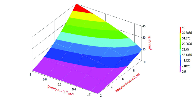
Figure 3: The interaction constant $g$.

The interaction constant $g$ as a function of the interlayer separation $D$ and exciton concentration $n$ is represented in Fig. 3. According to Fig. 3, the effective interaction constant $g$ increases with the increase of the interlayer separation $D$ and the increase of the exciton concentration $n$.

The mean field critical temperature $T_{c}$ for the excitonic superfluidity obtained from Eq. (77) is represented in Table 2. The critical temperature $T_{c}$ was calculated for different TMDC at the moderated concentration of excitons $n=3\times 10^{11}$ cm^-2, assuming $n_{A}=n_{B}=n/2$.

Table 2: Effective and reduced masses and factor $Q$ for two-component exciton gas of different TMDC materials at the interlayer separation $D=5\ \mathrm{nm}$.

	MoS2	MoSe2	MoTe2	WS2	WSe2	WTe2
$M_{A}+M_{B}$	1.044	1.180	1.766	0.722	0.802	0.778
$\mu_{AB}$	0.261	0.294	0.437	0.178	0.197	0.179
$Q$	15.380	13.655	9.260	22.750	20.769	24.453

Table 3: Dependence of the mean field critical temperature $T_{c}$ on the interlayer separation $D$ for different TMDC materials.

$D$, nm	$T_{c},$ K
	MoS2	MoSe2	MoTe2	WS2	WSe2	WTe2
2	22	21	19	25	24	26
3	38	36	32	43	41	44
4	55	53	47	63	61	64
5	74	71	63	85	82	87
6	95	91	80	108	105	110
7	116	112	98	132	128	136

Let us mention that for our calculations we substituted the exciton concentration $n=3\times 10^{11}$ cm^-2 smaller than the maximal exciton concentration obtained in the experiment You_bi : $n_{max}=5\times 10^{11}$ cm^-2. The exciton concentration $n=3\times 10^{11}$ cm^-2 used in our calculations corresponds to the degenerate exciton Bose gas in the phase diagram Fogler . While, in general, the electron-hole interaction is described by Keldysh’s potential Keldysh , we performed our calculations at the interlayer separation from $D=2\ \mathrm{nm}$ up to $D=10\ \mathrm{nm}$, when the screening effects are negligible, and the electron-hole interaction is described by Coulomb’s potential. We used for our calculations the interlayer separations $D$ larger than experimental values Calman by the following reasons: (i) the larger $D$ leads to the increase of the potential barrier for electron-hole tunneling between the layers, which results in the increase of the exciton life-time; (ii) the larger $D$ leads to the increase of the exciton dipole moment, which causes the increase of the exciton-exciton dipole-dipole repulsion, and, therefore, the increase of the sound velocity and the superfluid density, which results in the increase of the mean field temperature of the superfluidity, which can be seen in the Table 2.

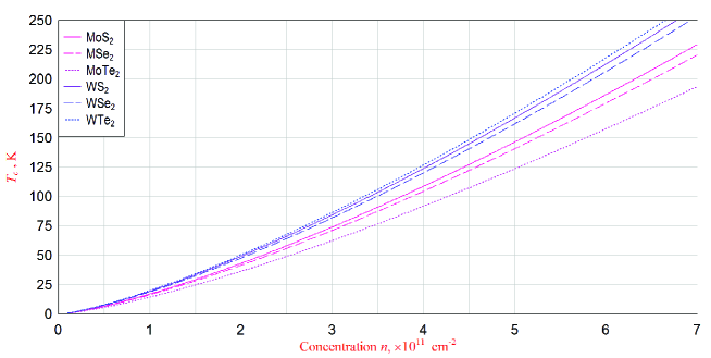
Figure 4: The mean field critical temperature of the superfluidity $T_{c}$ as a function of the exciton concentration $n$ for different TMDC materials at the interlayer separation $D=5\ \mathrm{nm}$.

The mean field critical temperature of the superfluidity $T_{c}$ as a function of the exciton concentration $n$ for MX₂ materials is represented in Fig. 4. According to Fig. 4, the critical temperature $T_{c}$ increases with the increase of the exciton concentration $n$, and $T_{c}$ is increased for different TMDC materials in the following order: $\mathrm{MoTe_{2}}$, $\mathrm{MoSe_{2}}$, $\mathrm{MoS_{2}}$, $\mathrm{WSe_{2}}$, $\mathrm{WS_{2}}$, $\mathrm{WTe_{2}}$. The critical temperature $T_{c}$ for all chalcogenides $\mathrm{Se}$, $\mathrm{S}$ and $\mathrm{Te}$ is larger for $\mathrm{WX_{2}}$ than for $\mathrm{MoX_{2}}$. It can be noticed that the order of types of different TMDC materials with respect to the increase of $T_{c}$, presented in Table 3 and Fig. 4, is exactly the same as the order of these TMDC materials with respect to the increase of the parameter $Q$, presented in Table 2. This is caused by the fact that, according to Eq. (77), $T_{c}$ is directly proportional to $Q^{1/3}$. Let us mention that the order of types of different TMDC materials with respect to the increase of $T_{c}$ is different from the order of these materials with respect to the exciton effective masses, presented in Table 1, and the parameters $a$, $t$, and the separation between $X$ planes $d_{X-X}$ taken from Ref. Kormanyos, .

The exciton-exciton interaction for studied in this Paper two-component weakly-interacting dilute system of A and B dipolar excitons leads to two branches of collective excitation spectrum characterized at small momenta by two different sound velocities $c_{1}$ and $c_{2}$, which is caused by the fact that the system under consideration is a two-component system. Therefore, at small temperatures the normal component is formed by the contributions from two types of quasiparticles, corresponding to two different branches of the collective excitations spectra with two different sound velocities at small momenta. All general expressions for the density of the normal and superfluid components and the mean-field phase transition temperature were calculated in this Paper, taking into account the existence of two branches of the spectrum of collective excitations. The calculations were presented for the specific case, when the concentrations of A and B excitons are equal, and the collective spectrum is characterized at small momenta by only one non-zero sound velocity.

We conclude that the critical temperature $T_{c}$ for superfluidity for two-component exciton gas in a TMDC bilayer is about one order of magnitude higher than $T_{c}$ for one-component exciton gas in the semiconductor coupled quantum wells. According to Eq. (77), the mean field critical temperature $T_{c}$ is directly proportional to the parameter $Q^{1/3}$, which is determined by the exciton reduced mass $\mu_{AB}$ and the sum of A and B exciton masses $M_{A}+M_{B}$, while for the one-component exciton Bose gas in CQWs $Q=M^{-1/3}$, where $M$ is the exciton mass in CQWs. For example, if $M_{A}$=$M_{B}$=$M$, then $Q$ for an one-component gas is eight times less than for a two-component Bose gas. Thus, for one-component dilute exciton gas $Q$ is always less than the value of $Q$ for a two-component Bose gas of A and B dipolar excitons. It can be easily seen that the inequalities $\mu_{AB}<M_{A}+M_{B}$ and $Q^{1/3}>\left(M_{A}+M_{B}\right)^{-1/3}$ are always true for any positive $M_{A}$ and $M_{B}$. Therefore, $T_{c}$ is always higher for a two-component dilute dipolar exciton gas than for any one-component dilute dipolar exciton gas in semiconductor CQWs in spite of the fact that the exciton masses for A and B excitons in CQWs are the same order of magnitude as exciton masses in CQWs. The advantage of the superfluidity of the dipolar excitons in a TMDC bilayer is in the possibility of the creating the superconducting electric currents in each TMDC layer by applying the external voltage, since electrons and holes in each monolayers are charge carriers. Since the quasiparticle gap and the exciton binding energy in TMDC can be tuned by externally applied voltage Chernikov_ef , the effective mass, the sound velocity for the collective excitations, the density of the superfluid component and the phase transition temperature for superfluidity can also be controlled by externally applied voltage.

VII Conclusions

We propose a physical realization to observe high-temperature superconducting electron-hole currents in two parallel TMDC layers which is caused by the superfluidity of quasi-two-dimensional dipolar A and B excitons in a TMDC bilayer. The effective exciton mass for A and B excitons is calculated analytically. The spectrum of collective excitations obtained in the Bogoliubov approximation for TMDC bilayer is characterized by two branches, reflecting the fact that the exciton system under consideration is a two-component weakly interacting Bose gas of A and B excitons. Two sound velocities for both branches of the collective spectrum are derived for two-component dipolar exciton system. It is shown that in the Bogolubov approximation the sound velocity in a two-component system is always larger than in an one-component system. The superfluid density, defined by the contributions from the collective excitations from two branches of collective spectrum, is obtained as a function of temperature for two-component system of A and B dipolar excitons. We show that the superfluid density and the mean-field phase transition temperature for superfluid increase with the increase of the excitonic concentration. The mean field critical temperature for the phase transition is analyzed for various TMDC materials. The mean field phase transition temperature, calculated for dipolar exciton bilayer, is about one order of magnitude higher than for any one-component exciton system of semiconductor CQWs due to the fact that $T_{c}$ for two-component exciton system in TMDC depends on the exciton reduced mass for the two-component system of A and B excitons, more exactly, depends on the factor $Q$, which is much larger for a two-component system than for an one-component exciton system.

Appendix A Eigenvalue problem for two particles

Let us introduce the following notations:

$$\mathcal{K}_{+} = \mathcal{K}\mathtt{e}^{i\Theta}=\mathcal{K}_{x}+i\mathcal{K}_{y}\ ,$$

$$\mathcal{K}_{-} = \mathcal{K}\mathtt{e}^{-i\Theta}=\mathcal{K}_{x}-i\mathcal{K}_{y}\ ,$$

$$\Theta = \tan^{-1}\left({\frac{\mathcal{K}_{y}}{\mathcal{K}_{x}}}\right)\ ,$$ (83)

and represent the Hamiltonian (17) in the form of a $2\times 2$ matrix as

$$\mathcal{H}_{\uparrow(\downarrow)}=\left({\ \begin{array}[]{cc}\mathcal{O}_{2}+V(r)\sigma_{0}-\frac{\Delta^{\prime}}{2}\sigma_{0}+\frac{\Delta^{\prime}}{2}\sigma_{3}&\mathcal{O}_{1}\\ \mathcal{O}_{1}^{\dagger}&\mathcal{O}_{2}+V(r)\sigma_{0}+\frac{\Delta^{\prime}}{2}\sigma_{0}+\frac{\Delta^{\prime}}{2}\sigma_{3}\end{array}}\right)\ ,$$ (86)

where $\mathcal{O}_{1}$ and $\mathcal{O}_{2}$ are given by

$$\mathcal{O}_{1} = at\left({\ \alpha\mathcal{K}_{-}-i\partial_{x}-\partial_{y}}\right)\sigma_{0},$$ (87)

$$\mathcal{O}_{2} = -at\left({\ \begin{array}[]{cc}0&\beta\mathcal{K}_{-}+i\partial_{x}+\partial_{y}\\ \beta\mathcal{K}_{+}+i\partial_{x}-\partial_{y}&0\end{array}}\right).$$ (90)

In Eqs. (A3) and (A4) $x$ and $y$ are the components of vector $\mathbf{r}$, $\sigma_{j}$ are the Pauli matrices, $\sigma_{0}$ is the $2\times 2$ unit matrix.

The eigenvalue problem (18) for the Hamiltonian (86) results in the following coupled equations:

$$\left({\mathcal{O}_{2}+V(r)\sigma_{0}-\frac{\Delta^{\prime}}{2}\sigma_{0}+\frac{\Delta^{\prime}}{2}\sigma_{3}}\right)\Psi_{c\uparrow(\downarrow)}+\mathcal{O}_{1}\Psi_{v\uparrow(\downarrow)} = \epsilon_{\uparrow(\downarrow)}\sigma_{0}\Psi_{c\uparrow(\downarrow)}$$

$$\mathcal{O}_{1}^{\dagger}\Psi_{c\uparrow(\downarrow)}+\left({\mathcal{O}_{2}+V(r)\sigma_{0}+\frac{\Delta^{\prime}}{2}\sigma_{0}+\frac{\Delta^{\prime}}{2}\sigma_{3}}\right)\Psi_{v\uparrow(\downarrow)} = \epsilon_{\uparrow(\downarrow)}\sigma_{0}\Psi_{v\uparrow(\downarrow)}\ .$$ (91)

It follows from Eq. (91) that

$$\Psi_{v\uparrow(\downarrow)}=\left({\epsilon_{\uparrow(\downarrow)}\sigma_{0}-\mathcal{O}_{2}-V(r)\sigma_{0}-\frac{\Delta^{\prime}}{2}\sigma_{0}-\frac{\Delta^{\prime}}{2}\sigma_{3}}\right)^{-1}\mathcal{O}_{1}^{\dagger}\Psi_{c\uparrow(\downarrow)}\ .$$ (92)

Assuming the electron-hole attraction potential energy and both relative and center-of-mass kinetic energies are small compared to the gap $\Delta^{\prime}$, the following approximation is applied:

$$\left(\epsilon_{\uparrow(\downarrow)}\sigma_{0}-\mathcal{O}_{2}-V(r)\sigma_{0}-\frac{\Delta^{\prime}}{2}\sigma_{0}-\frac{\Delta^{\prime}}{2}\sigma_{3}\right)^{-1}\simeq(\epsilon_{\uparrow(\downarrow)}\sigma_{0}-\frac{\Delta^{\prime}}{2}\sigma_{0}-\frac{\Delta^{\prime}}{2}\sigma_{3})^{-1}\ .$$ (93)

Applying

$$\mathcal{O}_{1}^{\dagger}\mathcal{O}_{1}=a^{2}t^{2}\left({\alpha^{2}\mathcal{K}^{2}-\nabla_{\mathbf{r}}^{2}-2i\alpha(\mathcal{K}_{x}\partial_{y}+\mathcal{K}_{y}\partial_{x})}\right)\sigma_{0}\ ,$$ (94)

and using Eq. (12) we obtain from Eq. (91) for the individual spinor components the following equations:

$$\left[V(r)+\frac{a^{2}t^{2}\left(\alpha^{2}\mathcal{K}^{2}-\nabla_{\mathbf{r}}^{2}-2i\alpha(\mathcal{K}_{x}\partial_{x}+\mathcal{K}_{y}\partial_{y})\right)}{\epsilon_{\uparrow(\downarrow)}-\Delta^{\prime}}\right]\phi_{c\uparrow(\downarrow)c\uparrow(\downarrow)}$$ (95)

$$- at\left({\beta\mathcal{K}_{-}+i\partial_{x}+\partial_{y}}\right)\phi_{c\uparrow(\downarrow)v\uparrow(\downarrow)}=\epsilon_{\uparrow(\downarrow)}\phi_{c\uparrow(\downarrow)c\uparrow(\downarrow)}\ ,$$

$$-at\left({\ \beta\mathcal{K}_{+}+i\partial_{x}-\partial_{y}}\right)\phi_{c\uparrow(\downarrow)c\uparrow(\downarrow)}$$ (96)

$$+ \left[V(r)-\Delta^{\prime}+\frac{a^{2}t^{2}\left(\alpha^{2}\mathcal{K}^{2}-\nabla_{\mathbf{r}}^{2}-2i\alpha\left(\mathcal{K}_{x}\partial_{x}+\mathcal{K}_{y}\partial_{y}\right)\right)}{\epsilon_{\uparrow(\downarrow)}}\right]\phi_{c\uparrow(\downarrow)v\uparrow(\downarrow)}=\epsilon_{\uparrow(\downarrow)}\phi_{c\uparrow(\downarrow)v\uparrow(\downarrow)}\ .$$

Following the procedure applied for calculation of the energy spectrum of the indirect excitons formed in two parallel gapped graphene layers BKZ , one gets from Eq. (95) for the spinor component

$$\phi_{c\uparrow(\downarrow)c\uparrow(\downarrow)}=-\left(\epsilon_{\uparrow(\downarrow)}-V(r)-\frac{a^{2}t^{2}\left(\alpha^{2}\mathcal{K}^{2}-\nabla_{\mathbf{r}}^{2}-2i\alpha\left(\mathcal{K}_{x}\partial_{x}+\mathcal{K}_{y}\partial_{y}\right)\right)}{\epsilon_{\uparrow(\downarrow)}-\Delta^{\prime}}\right)^{-1}\left(at\left(\beta\mathcal{K}_{-}+i\partial_{x}+\partial_{y}\right)\phi_{c\uparrow(\downarrow)v\uparrow(\downarrow)}\right)\ .$$ (97)

Assuming that the interaction potential and both the relative and center-of-mass kinetic energies are small compared to the exciton energy, we apply the following approximation:

$$\left[\epsilon_{\uparrow(\downarrow)}-V(r)-\frac{a^{2}t^{2}\left(\alpha^{2}\mathcal{K}^{2}-\nabla_{\mathbf{r}}^{2}-2i\alpha\left(\mathcal{K}_{x}\partial_{x}+\mathcal{K}_{y}\partial_{y}\right)\right)}{\epsilon_{\uparrow(\downarrow)}-\Delta^{\prime}}\right]^{-1}\approx\frac{1}{\epsilon_{\uparrow(\downarrow)}}\ .$$ (98)

Substituting $\phi_{c\uparrow(\downarrow)c\uparrow(\downarrow)}$ from Eq. (97) into Eq. (96) and applying the approximation given by Eq. (98), we obtain

$$\left[-\Delta^{\prime}+V(r)+\frac{a^{2}t^{2}\left(\beta^{2}\mathcal{K}^{2}-\nabla_{\mathbf{r}}^{2}+2i\beta\left(\mathcal{K}_{x}\partial_{x}+\mathcal{K}_{y}\partial_{y}\right)\right)}{\epsilon_{\uparrow(\downarrow)}}+\frac{a^{2}t^{2}\left(\alpha^{2}\mathcal{K}^{2}-\nabla_{\mathbf{r}}^{2}-2i\alpha\left(\mathcal{K}_{x}\partial_{x}+\mathcal{K}_{y}\partial_{y}\right)\right)}{\epsilon_{\uparrow(\downarrow)}}\right]\phi_{c\uparrow(\downarrow)v\uparrow(\downarrow)}$$ (99)

$$= \epsilon_{\uparrow(\downarrow)}\phi_{c\uparrow(\downarrow)v\uparrow(\downarrow)}\ .$$

Choosing the values for the coefficients $\alpha$ and $\beta$ to separate the coordinates of the center-of-mass (the wave vector $\mathcal{K}$ ) and relative motion $\mathbf{r}$ in Eq. (99), we have

$$\alpha=\frac{1}{2}\ ,\hskip 142.26378pt\beta=\frac{1}{2}\ .$$ (100)

Substituting Eq. (100) into Eq. (99), we get

$$\left[-\frac{2a^{2}t^{2}\nabla_{\mathbf{r}}^{2}}{\epsilon_{\uparrow(\downarrow)}}+\frac{a^{2}t^{2}\mathcal{K}^{2}}{2\epsilon}-\Delta^{\prime}+V(r)\right]\phi_{c\uparrow(\downarrow)v\uparrow(\downarrow)}=\epsilon_{\uparrow(\downarrow)}\phi_{c\uparrow(\downarrow)v\uparrow(\downarrow)}\ .$$ (101)

Appendix B Solution of the equation for the single exciton spectrum

Introducing $x=\sqrt{\epsilon_{\uparrow(\downarrow)}}$, we present Eq. (31) in the following form

$$2x^{4}+2\left(\Delta^{\prime}+V_{0}\right)x^{2}-\frac{8atN\sqrt{\gamma}x}{\sqrt{2}}-a^{2}t^{2}\mathcal{K}^{2}=0\ .$$ (102)

For small momenta $\hbar\mathcal{K}$, we assume

$$x=x_{0}+\Delta x\ ,$$ (103)

where $x=x_{0}$ corresponds to $\mathcal{K}=0$. In this case, we obtain from Eq. (102) the following equation:

$$x_{0}^{3}+\left(\Delta^{\prime}+V_{0}\right)x_{0}-\frac{4atN\sqrt{\gamma}}{\sqrt{2}}=0\ .$$ (104)

The cubic equation (104) has the following real root:

$$x_{0}=\left(\frac{q}{2}+\sqrt{\frac{q^{2}}{4}+\frac{p^{3}}{27}}\right)^{1/3}+\left(\frac{q}{2}-\sqrt{\frac{q^{2}}{4}+\frac{p^{3}}{27}}\right)^{1/3}\ ,$$ (105)

where the parameters $p$ and $q$ are given by

$$p=\Delta^{\prime}+V_{0}\ ,\hskip 142.26378ptq=\frac{4atN\sqrt{\gamma}}{\sqrt{2}}\ .$$ (106)

Substituting Eq. (103) into Eq. (102), in the first order with respect to $\Delta x$, we obtain

$$\Delta x=\frac{a^{2}t^{2}\mathcal{K}^{2}}{2C_{A(B)}}\ ,\hskip 85.35826ptC_{A(B)}=4x_{0}^{3}+2\left(\Delta^{\prime}+V_{0}\right)x_{0}-\frac{4atN\sqrt{\gamma}}{\sqrt{2}}\ ,$$ (107)

where $C_{A}$ and $C_{B}$ are related to the A and B excitons, when $\Delta^{\prime}=\Delta-\lambda$ and $\Delta^{\prime}=\Delta+\lambda$ are used for spin-down and spin-up particles, respectively. Let us also mention that the value of $x_{0}$ and $\Delta x$ are different for different TMDC material due to the values of parameters $a,$ $t$, $\Delta,$ and $\lambda.$ Using Eq. (104), we simplify Eq. (107) as

$$C_{A(B)}=3x_{0}^{3}+\left(\Delta^{\prime}+V_{0}\right)x_{0}\ .$$ (108)

Then we get for the exciton energy $\epsilon$ for A(B) exciton in the first order with respect to $\Delta x$:

$$\epsilon_{A(B)}=\epsilon_{\uparrow(\downarrow)}=\left(x_{0}+\Delta x\right)^{2}\approx x_{0}^{2}+2x_{0}\Delta x\ ,$$ (109)

where $x_{0}$ has the different value for A and B excitons.

References

- (1) S. N. Bose, Z. Phys. 26, 178 (1924).
- (2) A. Einstein, Sitzungsberich. Preussisch. Akad. Wissenschaft. 1, 3 (1925).
- (3) A. Griffin, Excitations in a Bose-condensed liquid (Cambridge University Press., Cambridge, UK, 1993).
- (4) L. Pitaevskii and S. Stringari, Bose-Einstein Condensation (Clarendon Press, Oxford, 2003).
- (5) M. H. Anderson and J. R. Ensher, Science 269, 198 (1995).
- (6) J. R. Ensher, D. S. Jin, M. R. Matthews, C. E. Wieman, and E. A. Cornell, Phys. Rev. Lett. 77, 4984 (1996).
- (7) W. Ketterle and N. J. Druten, Phys. Rev. A54, 656 (1996).
- (8) W. Ketterle and H.-J. Miesner, Phys. Rev. A56, 3291 (1997).
- (9) F. Daflovo, S. Giorgini, and L. P. Pitaevskii, Rev. Mod. Phys. 71, 463 (1999).
- (10) S. A. Moskalenko and D. W. Snoke, Bose-Einstein Condensation of Excitons and Biexcitons and Coherent Nonlinear Optics with Excitons (Cambridge University Press, New York, 2000).
- (11) Yu. E. Lozovik and V. I. Yudson, Sov. Phys. JETP 44, 389 (1976).
- (12) X. Zhu, P. B. Littlewood, M. S. Hybertsen, and T. M. Rice, Phys. Rev. Lett. 74, 1633 (1995).
- (13) G. Vignale and A. H. MacDonald, Phys. Rev. Lett. 76, 2786 (1996).
- (14) M. A. Olivares-Robles and S. E. Ulloa, Phys. Rev. B64, 115302 (2001).
- (15) D. W. Snoke, Science 298, 1368 (2002).
- (16) L. V. Butov, J. Phys. Condens. Matter 16, R1577 (2004).
- (17) J. P. Eisenstein and A. H. MacDonald, Nature (London) 432, 691 (2004).
- (18) O. L. Berman, Yu. E. Lozovik, D. W. Snoke, and R. D. Coalson, Phys. Rev. B70, 235310 (2004).
- (19) O. L. Berman, R. Ya. Kezerashvili, G. V. Kolmakov, and Yu. E. Lozovik, Phys. Rev. B86, 045108 (2012).
- (20) A. H. Castro Neto, F. Guinea, N. M. R. Peres, K. S. Novoselov, and A. K. Geim, Rev. Mod. Phys. 81, 109 (2009)
- (21) S. Das Sarma, S. Adam, E. H. Hwang, and E. Rossi, Rev. Mod. Phys. 83, 407 (2011).
- (22) Yu. E. Lozovik and A. A. Sokolik, JETP Lett. 87, 55 (2008).
- (23) C.-H. Zhang and Y. N. Joglekar, Phys. Rev. B77, 233405 (2008).
- (24) H. Min, R. Bistritzer, J.-J. Su, and A. H. MacDonald, Phys. Rev. B78, 121401(R) (2008).
- (25) R. Bistritzer and A. H. MacDonald, Phys. Rev. Lett. 101, 256406 (2008).
- (26) M. Yu. Kharitonov and K. B. Efetov, Phys. Rev. B78, 241401(R) (2008).
- (27) O. L. Berman, R. Ya. Kezerashvili, and K. Ziegler, Phys. Rev. B85, 035418 (2012).
- (28) A. Kormányos, G. Burkard, M. Gmitra, J. Fabian, V. Zólyomi, N. D. Drummond, and V. Fal’ko, 2D Mater. 2, 022001 (2015).
- (29) K. F. Mak, C. Lee, J. Hone, J. Shan, and T. F. Heinz, Phys. Rev. Lett. 105, 136805 (2010).
- (30) K. F. Mak, K. He, J. Shan, and T. F. Heinz, Nat. Nanotechnol. 7, 494 (2012).
- (31) L. Britnell, R. M. Ribeiro, A. Eckmann, R. Jalil, B. D. Belle, A. Mishchenko, Y.-J. Kim, R. V. Gorbachev, T. Georgiou, S. V. Morozov, A. N. Grigorenko, A. K. Geim, C. Casiraghi, A. H. Castro Neto, and K. S. Novoselov, Science 340, 1311 (2013).
- (32) W. Zhao, Z. Ghorannevis, L. Chu, M. Toh, C. Kloc, P.-H. Tan, and G. Eda, ACS Nano 7, 791 (2013).
- (33) D. Xiao, G.-B. Liu, W. Feng, X. Xu, and W. Yao, Phys. Rev. Lett. 108, 196802 (2012).
- (34) T. Cao, et al., Nat. Commun. 3, 887 (2012).
- (35) J. S. Ross, S. Wu, H. Yu, N. J. Ghimire, A. M. Jones, G. Aivazian, J. Yan, D. G. Mandrus, D. Xiao, W. Yao, and X. Xu, Nat. Commun. 4, 1474 (2013).
- (36) K. F. Mak, et al., Nat. Mater. 12, 207 (2013).
- (37) R. A. Bromley, R. B. Murray, and A. D. Yoffe, J. Phys. C 5, 759 (1972).
- (38) R. A. Bromley and R. B. Murray, J. Phys. C 5, 738 (1972).
- (39) L. F. Mattheis, Phys. Rev. B8, 3719 (1973).
- (40) T. Cheiwchanchamnangij and W. R. L. Lambrecht, Phys. Rev. B85, 205302 (2012).
- (41) A. Ramasubramaniam, Phys. Rev. B86, 115409 (2012).
- (42) A. Molina-Sánchez, D. Sangalli, K. Hummer, A. Marini, and L. Wirtz, Phys. Rev. B88, 045412 (2013).
- (43) F. Hüser, T. Olsen, and K. S. Thygesen, Phys. Rev. B88, 245309 (2013).
- (44) G. Berghäuser and E. Malic, Phys. Rev. B89, 125309 (2014).
- (45) A. Chernikov, T. C. Berkelbach, H. M. Hill, A. Rigosi, Y. Li, O. B. Aslan, D. R. Reichman, M. S. Hybertsen, and T. F. Heinz, Phys. Rev. Lett. 113, 076802 (2014).
- (46) F. Wu, F. Qu, and A. H. MacDonald, Phys. Rev. B91, 075310 (2015).
- (47) H.-P. Komsa and A. V. Krasheninnikov, Phys. Rev. B86, 241201(R) (2012).
- (48) H. Shi, H. Pan, Y.-W. Zhang, and B. I. Yakobson, Phys. Rev. B87, 155304 (2013).
- (49) T. C. Berkelbach, M. S. Hybertsen, and D. R. Reichman, Phys. Rev. B88, 045318 (2013).
- (50) A. Ramirez-Torres, V. Turkowski, and T. S. Rahman, Phys. Rev. B90, 085419 (2014).
- (51) T. C. Berkelbach, M. S. Hybertsen, and D. R. Reichman, Phys. Rev. B92, 085413 (2015).
- (52) M. M. Fogler, L. V. Butov, and K. S. Novoselov, Nature Commun. 5, 4555 (2014).
- (53) E. V. Calman, C. J. Dorow, M. M. Fogler, L. V. Butov, S. Hu, A. Mishchenko, and A. K. Geim, arXiv: 1510.04410 (2015).
- (54) F. Ceballos, M. Z. Bellus, H.-Y. Chiu, and H. Zhao, ACS Nano 8, 12717 (2014).
- (55) G. Wang, X. Marie, L. Bouet, M. Vidal, A. Balocchi, T. Amand, D. Lagarde, and B. Urbaszek, Appl. Phys. Lett. 105, 182105 (2014).
- (56) D. S. Jin, M. R. Matthews, J. R. Ensher, C. E. Wieman, and E. A. Cornel, Phys. Rev. Lett. 78, 764 (1997).
- (57) P. Öhberg and S. Stenholm, Phys. Rev. A57, 1272 (1998).
- (58) E. Altman, W. Hofstetter, E. Demler, and M. D. Lukin, New Journal of Physics 5, 113 (2003).
- (59) K. Kasamatsu, M. Tsubota, and M. Ueda, Phys. Rev. Lett. 91, 150406 (2003).
- (60) P. Tommasini, E. J. V. de Passos, A. F. R. de Toledo Piza, M. S. Hussein, and E. Timmermans, Phys. Rev. A67, 023606 (2003).
- (61) C.-Y. Lin, E. J. V. de Passos, A. F. R. de Toledo Piza, D.-S. Lee, and M. S. Hussein, Phys. Rev. A73, 013615 (2006).
- (62) B. Sun and M. S. Pindzola, J. Phys. B 43 055301 (2010).
- (63) A. A. Abrikosov, L. P. Gorkov, and I. E. Dzyaloshinskii, Methods of Quantum Field Theory in Statistical Physics(Prentice-Hall, Englewood Cliffs, NJ, 1963).
- (64) E. M. Lifshitz and L. P. Pitaevskii, Statistical Physics, Part 2 (Pergamon Press, Oxford, 1980).
- (65) D. Y. Qiu, F. H. da Jornada, and S. G. Louie, Phys. Rev. Lett. 111, 216805 (2013).
- (66) L. V. Keldysh, JETP Lett. 29, 658 (1979).
- (67) P. Cudazzo, I. V. Tokatly, and A. Rubio, Phys. Rev. B84, 085406 (2011).
- (68) O. L. Berman, R. Ya. Kezerashvili, and K. Ziegler, Phys. Rev. A87, 042513 (2013).
- (69) J. Sabio, F. Sols, and F. Guinea, Phys. Rev. B81, 045428 (2010).
- (70) Y. You, X.-X. Zhang, T. C. Berkelbach, M. S. Hybertsen, D. R. Reichman, and T. F. Heinz, Nature Physics. 11, 477 (2015).
- (71) O. L. Berman, R. Ya. Kezerashvili, and Yu. E. Lozovik, Phys. Rev. B78, 035135 (2008).
- (72) O. L. Berman, R. Ya. Kezerashvili, and Yu. E. Lozovik, Phys. Lett. A 372, 6536 (2008).
- (73) C. Ciuti, V. Savona, C. Piermarocchi, A. Quattropani, and P. Schwendimann, Phys. Rev. B58, 7926 (1998).
- (74) S. Ben-Tabou de-Leon and B. Laikhtman, Phys. Rev. B63, 125306 (2001).
- (75) C. Ciuti, P. Schwendimann, and A. Quattropani, Semicond. Sci. Technol. 18 S279 (2003).
- (76) O. L. Berman, R. Ya. Kezerashvili, and K. Ziegler, Phys. Rev. B86, 235404 (2012).
- (77) X. Liu, T. Galfsky, Z. Sun, F. Xia, E.-C. Lin, Y.-H. Lee, Stéphane Kéna-Cohen, and V. M. Menon, Nature Photonics 9, 30 (2015).
- (78) A. Chernikov, A. M. van der Zande, H. M. Hill, A. F. Rigosi, A. Velauthapillai, J. Hone, and T. F. Heinz, Phys. Rev. Lett. 115, 126802 (2015).