Duality symmetries behind solutions of the classical simple pendulum

Abstract

The solutions that describe the motion of the classical simple pendulum have been known for very long time and are given in terms of elliptic functions, which are doubly periodic functions in the complex plane. The independent variable of the solutions is time and it can be considered either as a real variable or as a purely imaginary one, which introduces a rich symmetry structure in the space of solutions. When solutions are written in terms of the Jacobi elliptic functions the symmetry is codified in the functional form of its modulus, and is described mathematically by the six dimensional coset group $\Gamma/\Gamma(2)$ where $\Gamma$ is the modular group and $\Gamma(2)$ is its congruence subgroup of second level. In this paper we discuss the physical consequences this symmetry has on the pendulum motions and it is argued they have similar properties to the ones termed as duality symmetries in other areas of physics, such as field theory and string theory. In particular a single solution of pure imaginary time for all allowed value of the total mechanical energy is given and obtained as the $S$-dual of a single solution of real time, where $S$ stands for the $S$ generator of the modular group.

I Introduction

The simple plane pendulum constitutes an important physical system whose analytical solutions are well known. Historically the first systematic study of the pendulum is attributed to Galileo Galilei, around 1602. Thirty years later he discovered that the period of small oscillations is approximately independent of the amplitude of the swing, property termed as isochronism, and in 1673 Huygens published the mathematical formula for this period. However, as soon as 1636, Marin Mersenne and René Descartes had stablished that the period in fact does depend of the amplitude Matthews (1994). The mathematical theory to evaluate this period took longer to be established.

The Newton second law for the pendulum leads to a nonlinear differential equation of second order whose solutions are given in terms of either Jacobi elliptic functions or Weierstrass elliptic functions Whittaker and Watson (1927); Du Val (1973); Lang (1973); Lawden (1989); McKean and Moll (1999); Armitage and Eberlein (2006). There are several textbooks on classical mechanics Appell (1897); Von Helmholtz and Krigar-Menzel (1898); Whittaker (1917), and recent papers Beléndez et al. (2007); Brizard (2009); Ochs (2011), that give account of these solutions. From the mathematical point of view the subject of interest is the one of elliptic curves such as $y^{2}=(1-x^{2})(1-k^{2}x^{2})$, with $k^{2}\neq 0,1$, the corresponding elliptic integrals $\int_{0}^{x}dx/y$ and the elliptic functions which derive from the inversion of them. Generically the domain of the elliptic functions is the complex plane $\mathbb{C}$ and they depend also on the value of the modulus $k$. The theory began to be studied in the mid eighteenth century and involved great mathematicians such as Fagnano, Euler, Gauss and Lagrange. The cornerstone in its development is due to Abel Abel (1827) and Jacobi Jacobi (1827, 1829), who replaced the elliptic integrals by the elliptic functions as the object of study. Since then they both are recognized jointly as the mathematicians that developed the elliptic functions theory in their current form and to the theory itself as one of the jewels of nineteen-century mathematics.

Because the solutions to the simple pendulum problem are given in terms of elliptic functions and the founder fathers of the subject taught us all the interesting properties of these functions, it can be concluded that all the characteristics of the different type of motions of the pendulum are known. This is strictly true, however most of the references on elliptic functions (see for instance Whittaker and Watson (1927); Du Val (1973); Lang (1973); Lawden (1989); McKean and Moll (1999); Armitage and Eberlein (2006) and references therein) focus, as it should be, on its mathematical properties, applying just some of them to the simple pendulum as an example. In this paper we review part of the analysis made by Klein Klein (1890), who studied the properties that the transformations of the modular group $\Gamma$ and its congruence subgroups of finite index $\Gamma(N)$ have on the modular parameter $\tau$, being the latter a function of the quarter periods $K$ and $K_{c}$ which in turn are determined by the value of the square modulus $k^{2}$. Our main interest in this paper is accentuate the physical meaning that these transformations have in the specific case of the simple pendulum, in our opinion this is a piece of analysis missing in the literature.

For our purposes the relevant mathematical result is that the congruence subgroup of level 2, denoted as $\Gamma(2)$, is of order six in $\Gamma$ and therefore a fundamental cell for $\Gamma(2)$ can be formed from six copies of any fundamental region ${\cal F}$ of $\Gamma$ produced by the action of the six elements on the set of modular parameters $\tau$ that belong to ${\cal F}$. Each of these copies is distinguished from each other, according to the functional form of the modulus $k^{2}$ the six transformations leave invariant, being they: $k^{2}$, $1-k^{2}$, $1/k^{2}$, $1-1/k^{2}$, $1/(1-k^{2})$ and $k^{2}/(k^{2}-1)$, interestingly these kind of relations appear in other areas of physics under the concept of duality transformations, nomenclature we will use here. This result can be understood from different mathematical points of view and provides a link between concepts such as lattices, complex structures on the topological torus ${\mathbb{T}}^{2}$, the modular group $\Gamma$ and elliptic functions. In the appendices we review briefly the basics of these concepts in order to keep the paper self contained as possible, emphasizing in every moment its role in the solutions of the simple pendulum. From the physical point of view, the pendulum can follow basically two kind of motions (with the addition of some limit situations), the specific type of motion depends entirely on the value of the total mechanical energy $k^{2}_{E}$, if $0<k^{2}_{E}<1$ the motion is oscillatory and if $1<k^{2}_{E}<\infty$ the motion is circulatory. Therefore in the problem of the simple pendulum, there are two relevant parameters, the square modulus $k^{2}$ of the elliptic functions that parameterize its solutions in terms of the time variable, and the total mechanical energy of the motion $k^{2}_{E}$. As we will discuss throughout the paper, the relation between these two parameters is not one-to-one due to the duality relations between the different invariant functional forms of $k^{2}$. For instance, for an oscillatory motion whose energy is $0<k^{2}_{E}<1$, it is possible to express the solution in terms of an elliptic Jacobi function whose square modulus is $k^{2}$, $1-k^{2}$, $1/k^{2}$, etc., in other words, the duality symmetries between the functional forms of the square modulus $k^{2}$ induce different equivalent ways to write the solution for an specific physical motion of the pendulum. The nature of the time variable also plays an important role in the equivalence of solutions, it turns out that whereas some solutions are functions of a real time, others are functions of a pure imaginary time. In this paper we will discuss all these issues and we will write down explicitly several equivalent solutions to describe an specific pendulum motion. These results constitute an example in classical mechanics of a broader concept in physics termed under the name dualities. It is worth mentioning that many of the results we present here are already scattered throughout the mathematical literature but our exposition collects them together and is driven by a golden rule in physics that demands to explore all the physical consequences from symmetries. Notwithstanding some formulas have been worked out specifically for building up the arguments given in here and to the best knowledge of the author they are not present in the available literature. As an example, we obtain a single solution that describes the motions of the simple pendulum as function of a pure imaginary time parameter, and we show it can be obtained through an $S$-duality transformation from a single formula that describes the motions of the simple pendulum for all permissible value of the total energy and which is function of a real time variable..

In a general context the duality symmetries we refer to, involve the special linear group $SL(2,\mathbb{Z})$ and appear often in physics either as an invariance of a theory or as a relationship among two different theories. Typically these discrete symmetries relate strong coupled degrees of freedom to weakly coupled ones and vice versa, and the relationship is useful when one of the two systems so related can be analyzed, permitting conclusions to be drawn for its dual by acting with the duality transformations. There is a plethora of examples in physics that obey duality symmetries, which have led to important developments in field theory, gravity, statistical mechanics, string theory etc. (for an explicit account of examples see for instance Petropoulos and Vanhove (2012) and references therein). As a manner of illustration let us mention just two examples of theories that own duality symmetries: i) in string theory appear three types of dualities, and the one that have the properties described above goes by the name $S$-duality, being the $S$ group element, one of the two generators of the group $SL(2,\mathbb{Z})$ Schwarz (1997). In this case the modular parameter $\tau$ is given by the coupling constant and therefore the $S$-duality relates the strong coupling regime of a given string theory to the weak coupling one of either the same string theory or another string theory. It is conjectured for instance that the type I superstring is $S$-dual to the $SO(32)$ heterotic superstring, and that the type $IIB$ superstring is $S$-dual to itself. ii) In 2D systems there is a broad class of dual relationships for which the electromagnetic response is governed by particles and vortices whose properties are similar. In particular for systems having fermions as the particles (or those related to fermions by the duality) the vortex-particle duality implies the duality group is the level-two subgroup $\Gamma_{0}(2)$ of $PSL(2,\mathbb{Z})$ Burgess and Dolan (2001). The so often appearance of these duality symmetries in physics is our main motivation to heighten the fact that in classical mechanics there are also systems like the simple pendulum whose motions are related by duality symmetries.

The structure of the paper is as follows. In section II we summarize the real time solutions of the simple pendulum system in terms of elliptical Jacobi functions. The relations between solutions with real time and pure imaginary time in terms of the $S$ group element of the modular group $\Gamma$ are exemplified in section III and the whole web of dualities is discussed in section IV. We make some final remarks in V. There are two appendices, appendix A is dedicated to define the modular group, its congruence subgroups and its relation to double lattices whereas in appendix B we give some properties of the elliptic Jacobi functions that are relevant for the analysis of the solutions of the simple pendulum.

II Real time solutions

The Lagrangian for a pendulum of point mass $m$ and length $l$, in a constant downwards gravitational field, of magnitude $-g$ ($g>0$), is given by

$$L(\theta,\dot{\theta})=\frac{1}{2}ml^{2}\dot{\theta}^{2}-mgl(1-\cos\theta),$$ (1)

where $\theta$ is the polar angle measured counterclockwise respect to the vertical line and $\dot{\theta}$ stands for the time derivative of this angular position. Here the zero of the potential energy is set at the lowest vertical position of the pendulum, for which $\theta=2n\pi$, with $n\in\mathbb{Z}$. The equation of motion for this system is

$$\ddot{\theta}+\frac{g}{l}\sin\theta=0.$$ (2)

This equation can be integrated once giving origin to a first order differential equation, whose physical meaning is the conservation of energy

$$E=\frac{1}{2}ml^{2}\dot{\theta}^{2}+2mgl\sin^{2}\left(\frac{\theta}{2}\right)=constant.$$ (3)

Physical solutions exist only if $E\geq 0$. We can rewrite this equation of conservation, in dimensionless form, in terms of the dimensionless energy parameter: $k_{E}^{2}\equiv\frac{E}{2mgl}$, and the dimensionless real time variable: $x\equiv\sqrt{\frac{g}{l}}t\in\mathbb{R}$, obtaining

$$\frac{1}{4}\left(\frac{d\theta}{dx}\right)^{2}+\sin^{2}\left(\frac{\theta}{2}\right)=k_{E}^{2}.$$ (4)

Analyzing the potential, it is concluded that the pendulum has four different types of solutions depending of the value of the constant $k_{E}^{2}$. The analytical solutions in two of the four cases are given in terms of Jacobi elliptic functions and can be found for instance in Lawden (1989); Armitage and Eberlein (2006); Appell (1897); Von Helmholtz and Krigar-Menzel (1898); Whittaker (1917); Beléndez et al. (2007); Brizard (2009); Ochs (2011). The other two cases can be considered just as limit situations of the previous two. The Jacobi elliptic functions are doubly periodic functions in the complex $z$-plane (see appendix B for a short summary of the basic properties of these functions), for example, the function $\mbox{sn}(z,k)$ of square modulus $0<k^{2}<1$, has the real primitive period $4K$ and the pure imaginary primitive period $2iK_{c}$, where the so called quarter periods $K$ and $K_{c}$ are defined by the equations (45) and (48) respectively. The properties of the different solutions are as follows:

$\bullet$ Static equilibrium ($\dot{\theta}=0$): The trivial behavior occurs when either $k_{E}^{2}=0$ or $k_{E}^{2}=1$. In the first case, necessarily $\dot{\theta}=0$. For the case $k_{E}^{2}=1$ we consider also the situation where $\dot{\theta}=0$. In both cases, the pendulum does not move, it is in static equilibrium. When $\theta=2n\pi$ the equilibrium is stable and when $\theta=(2n+1)\pi$ the equilibrium is unstable.

$\bullet$ Oscillatory motions ($0<k_{E}^{2}<1$): In these cases the pendulum swings to and fro respect to a point of stable equilibrium. The analytical solutions are given by

$$\theta(x) = 2\arcsin[k_{E}\,\mbox{sn}(x-x_{0},k_{E})],$$ (5)

$$\frac{d\theta}{dx}\equiv\omega(x) = 2\,k_{E}\,\mbox{cn}(x-x_{0},k_{E}),$$ (6)

where the square modulus $k^{2}$ of the elliptic functions is given directly by the energy parameter: $k^{2}\equiv k^{2}_{E}$. Here $x_{0}$ is a second constant of integration and appears when equation (4) is integrated out. It means physically that we can choose the zero of time arbitrarily. Derivatives of the basic Jacobi elliptic functions are given in (54).

Without loose of generality, in our discussion we consider that the lowest vertical point of the oscillation corresponds to the angular value $\theta=0$, and therefore that $\theta$ takes values in the closed interval $[-\theta_{m},\theta_{m}]$, where $0<\theta_{m}<\pi$ is the angle for which $\dot{\theta}_{m}=0$. This means that: $\sin(\theta/2)\in[-\sin(\theta_{m}/2),\sin(\theta_{m}/2)]$, where according to equation (4), $\sin^{2}(\theta_{m}/2)=k^{2}_{E}<1$. Now according to (5) the solution is obtained by mapping : $\sin(\theta/2)\rightarrow k_{E}\,\mbox{sn}(x-x_{0},k_{E})$, where $x-x_{0}\in[-K,K]$, or equivalently: $\mbox{sn}(x-x_{0},k_{E})\in[-1,1]$. With this map we describe half of a period of oscillation. To describe the another half, without loose of generality, we can extend the mapping in such a way that for a complete period of oscillation, $x-x_{0}\in[-K,3K]$. Because the Jacobi function cn$(x-x_{0},k_{E})\in[-1,1]$, the dimensionless angular velocity $\omega(x)$ is restricted to values in the interval $[-2k_{E},2k_{E}]$.

Figure 1: The first set of graphs represents an oscillatory motion of energy $k_{E}^{2}=3/4$ with $x_{0}=K\approx 2.1565$. $\theta(x)$ is given by the magenta graph and it oscillates in the interval $\theta(x)\in[-2\pi/3,2\pi/3]$. The angular velocity $\omega(x)$ is showed in blue and takes values in the interval $\omega(x)\in[-\sqrt{3},\sqrt{3}]$. Both graphs have period $4K$. The second set of graphs represents a couple of circulating motions both of energy $k_{E}^{2}=4/3$ with $x_{0}=K/k_{E}\approx 1.8676$. For the motion in the counterclockwise direction, the monotonic increasing function $\theta(x)$ is plotted in magenta, for the time interval $x\in[0,2x_{0})$ it takes values in the interval $\theta(x)\in[-\pi,\pi)$, whereas for the interval $x\in[2x_{0},4x_{0})$ it takes values in the interval $\theta(x)\in[\pi,3\pi)$. The angular velocity is showed in blue, it has period $2K/k_{E}$, is always positive and takes values in the interval $\omega(x)\in[2/\sqrt{3},4/\sqrt{3}]$. The other two plots represent a similar motion in the clockwise direction.

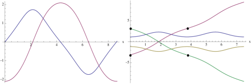
As an example we can choose $x_{0}=K$, so at the time $x=0$, the pendulum is at minimum angular position $\theta(0)=-\theta_{m}$, with angular velocity $\omega(0)=0$. The pendulum starts moving from left to right, so at $x=K$ it reaches the lowest vertical position $\theta(K)=0$ at highest velocity $\omega(K)=2k_{E}$ and at $x=2K$ it is at maximum angular position $\theta(2K)=\theta_{m}$ with velocity $\omega(2K)=0$. At this very moment the pendulum starts moving from right to left, so at $x=3K$ it is again at $\theta(3K)=0$ but now with lowest angular velocity $\omega(3K)=-2k_{E}$ and it completes an oscillation at $x=4K$ when the pendulum reaches again the point $\theta(4K)=-\theta_{m}$ with zero velocity (see figure 1). We can repeat this process every time the pendulum swings in the interval $[-\theta_{m},\theta_{m}]$, in such a way that the argument of the elliptic function $\mbox{sn}(x,k_{E})$, becomes defined in the whole real line $\mathbb{R}$. It is clear that the period of the movement is $4K$, or restoring the dimension of time, $4K\sqrt{g/l}$.

Of course the value of $x_{0}$ can be set arbitrarily and it is also possible to parameterize the solution in such a way that at zero time $x=0$, the motion starts in the angle $\theta_{m}$ instead of $-\theta_{m}$. In this case the mapping of a complete period of oscillation can be defined for instance in the interval $x-x_{0}\in[K,5K]$ and the initial condition can be taken as $x_{0}=-K$. In the discussion of the following section we will set $x_{0}=0$, so at time $x=0$, the pendulum is at the lowest vertical position ($\theta(0)=0$) moving from left to right.

$\bullet$ Asymptotical motion ($k_{E}^{2}=1$ and $\dot{\theta}\neq 0$): In this case the angle $\theta$ takes values in the open interval $(-\pi,\pi)$ and therefore, $\sin(\theta/2)\in(-1,1)$. The particle just reach the highest point of the circle. The analytical solutions are given by

$$\theta(x) = \pm 2\arcsin[\tanh(x-x_{0})],$$ (7)

$$\omega(x) = \pm 2\,\mbox{sech}(x-x_{0}).$$ (8)

The sign $\pm$ corresponds to the movement from $(\mp\pi\rightarrow\pm\pi)$. Notice that $\tanh(x-x_{0})$, takes values in the open interval $(-1,1)$ if: $x-x_{0}\in(-\infty,\infty)$. For instance if $\theta\rightarrow\pi$, $x-x_{0}\rightarrow\infty$ and $\tanh(x-x_{0})$ goes asymptotically to 1. It is clear that this movement is not periodic. In the literature it is common to take $x_{0}=0$.

$\bullet$ Circulating motions ($k_{E}^{2}>1$): In these cases the momentum of the particle is large enough to carry it over the highest point of the circle, so that it moves round and round the circle, always in the same direction. The solutions that describe these motions are of the form

$$\theta(x) = \pm 2\,\mbox{sgn}\left[\mbox{cn}\left(k_{E}(x-x_{0}),\frac{1}{k_{E}}\right)\right]\arcsin\left[\mbox{sn}\left(k_{E}(x-x_{0}),\frac{1}{k_{E}}\right)\right],$$ (9)

$$\omega(x) = \pm 2\,k_{E}\,\mbox{dn}\left(k_{E}(x-x_{0}),\frac{1}{k_{E}}\right),$$ (10)

where the global sign $(+)$ is for the counterclockwise motion and the $(-)$ sign for the motion in the clockwise direction. The symbol sgn$(x)$ stands for the piecewise sign function which we define in the form

$$\mbox{sgn}\left[\mbox{cn}\left(k_{E}(x-x_{0}),\frac{1}{k_{E}}\right)\right]=\left\{\begin{array}[]{cc}+1&\mbox{if}\,\,\,\,\,(4n-1)K\leq k_{E}(x-x_{0})<(4n+1)K,\\ -1&\mbox{if}\,\,\,\,\,(4n+1)K\leq k_{E}(x-x_{0})<(4n+3)K,\end{array}\right.$$ (11)

and its role is to shorten the period of the function sn$(k_{E}(x-x_{0}),1/k_{E})$ by half, as we argue below. This fact is in agreement with the expression for the angular velocity $\omega(x)$ because the period of the elliptic function dn$(k_{E}(x-x_{0}),1/k_{E})$ is $2K/k_{E}$ instead of $4K/k_{E}$ that is the period of the elliptic function sn$(k_{E}(x-x_{0}),1/k_{E})$.

The square modulus $k^{2}$ of the elliptic functions is equal to the inverse of the energy parameter $0<k^{2}=1/k_{E}^{2}<1$. Without loosing generality we can assume both that $k_{E}(x-x_{0})\in[-K,K)$, where $K$ is defined in (45) and evaluated for $k^{2}=1/k^{2}_{E}$ and that arcsin[sn$(k_{E}(x-x_{0}),1/k_{E})]\in[-\pi/2,\pi/2)$. Because in this interval the function sgn[cn$(k_{E}(x-x_{0}),1/k_{E})]=1$, the angular position function $\theta(x)\in[\mp\pi,\pm\pi)$ for the global sign ($\pm$) in (9). As for the interval $k_{E}(x-x_{0})\in[K,3K)$, we can consider that the function arcsin[sn$(k_{E}(x-x_{0}),1/k_{E})]\in(-3\pi/2,-\pi/2]$, and because the function sgn[cn$(k_{E}(x-x_{0}),1/k_{E})]=-1$, it reflects the angular position interval, obtaining finally that $\theta\in[\pm\pi,\pm 3\pi)$ for the global ($\pm$) sign in (9) (see figure 1). We stress that the consequence of flipping the sign of the angular interval through the sgn function is to make the function $\theta(x)$ piecewise periodic, whereas the consequence of taking a different angular interval for the image of the arcsin function every time its argument changes from an increasing to a decreasing function and vice versa, is to make the function $\theta(x)$ a continuous monotonic increasing (decreasing) function for the global sign + (-). Explicitly the angular position function changes as

$$\theta\left(x+n\frac{2K}{k_{E}}\right)=\theta(x)\pm 2\pi n.$$ (12)

It is interesting to notice that if we would not have changed the image of the arcsin function, the angular position function $\theta(x)$ would have resulted into a piecewise function both periodic and discontinuous.

The angular velocity is a periodic function whose period is given by $T_{circulating}=2(K/k_{E})\sqrt{g/l}$ which means as expected that higher the energy, shorter the period. Because the image of the Jacobi function dn$(x,k)\in[\sqrt{1-1/k_{E}^{2}},1]$, the angular velocity takes values in the interval $|\omega|\in[2\sqrt{k_{E}^{2}-1},2|k_{E}|]$. An interesting property of the periods that follows from solutions (6) and (10) is that $T_{oscillatory}=k_{E}T_{circulating}$ where $k_{E}^{2}$ is the energy of a circulating motion and $k^{2}=1/k_{E}^{2}$ is the modulus used to compute $K$ in both cases. This is a clear hint that a relation between circulating and oscillatory solutions exists.

These are all the possible motions of the simple pendulum. It is straightforward to check that the solutions satisfy the equation of conservation of energy (4) by using the following relations between the Jacobi functions (in these relations the modulus satisfies $0<k^{2}<1$) and its analogous relation for hyperbolic functions (which is obtained in the limit case $k=1$)

$$\mbox{sn}^{2}(x,k)+\mbox{cn}^{2}(x,k) = 1,$$ (13)

$$\tanh^{2}(x)+\mbox{sech}^{2}(x) = 1,$$ (14)

$$k^{2}\mbox{sn}^{2}(x,k)+\mbox{dn}^{2}(x,k) = 1.$$ (15)

III Imaginary time solutions and $S$-duality

The argument $z$ of the Jacobi elliptic functions is defined in the whole complex plane $\mathbb{C}$ and the functions are doubly periodic (see appendix B), however in the analysis above, time was considered as a real variable, and therefore in the solutions of the simple pendulum only the real quarter period $K$ appeared. In 1878 Paul Appell clarified the physical meaning of the imaginary time and the imaginary period in the oscillatory solutions of the pendulum Appell (1878); Armitage and Eberlein (2006), by introducing an ingenious trick, he reversed the direction of the gravitational field: $g\rightarrow-g$, i.e. now the gravitational field is upwards. In order the Newton equations of motion remain invariant under this change in the force, we must replace the real time variable $t$ by a purely imaginary one: $\tau\equiv\pm it$. Implementing these changes in the equation of motion (2) leads to the equation

$$\frac{d^{2}\theta}{d\tau^{2}}-\frac{g}{l}\sin\theta=0.$$ (16)

Writing this equation in dimensionless form requires the introduction of the pure imaginary time variable $y\equiv\pm\tau\sqrt{g/l}=\pm ix$. Integrating once the resulting dimensionless equation of motion gives origin to the following equation

$$\frac{1}{4}\left(\frac{d\theta}{dy}\right)^{2}-\sin^{2}\left(\frac{\theta}{2}\right)=E^{\prime},$$ (17)

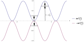
which looks like equation (4) but with an inverted potential (see figure 2).

Figure 2: In the figure we show the pendulum potential (blue) for the dynamical motion parameterized with a real time variable. The inverted potential (magenta) corresponds to a dynamics parameterized by a pure imaginary time variable.

We can solve the equation in two different but equivalent ways: i) the first option consists in writing down the equation in terms of a real time variable and then flipping the sign of the whole equation in order to have positive energies, the resulting equation is of the same form as equation (4), ii) the second option consists in solving the equation directly in terms of the imaginary time $y$. Because both solutions describe to the same physical system, we can conclude that both are just different representations of the same physics. These two-ways of working provide relations between the elliptic functions with different argument and different modulus. As we will discuss the relations among different time variables and modulus can be termed as duality relations and because the mathematical group operation beneath these relations is the $S$ generator of the modular group $PSL(2,\mathbb{Z})$, we can refer to this duality relation as $S$-duality.

III.1 Real time variable

If we write down (17) explicitly in terms of the real time parameter $x$, we obtain a conservation equation of the form

$$-\frac{1}{4}\left(\frac{d\theta}{dx}\right)^{2}-\sin^{2}\left(\frac{\theta}{2}\right)=E^{\prime}.$$ (18)

The first feature of this equation is that the constant $E^{\prime}$ is negative $(E^{\prime}<0)$. This happens because as a consequence of the imaginary nature of time, the momentum also becomes an imaginary quantity and when it is written in terms of a real time it produces a negative kinetic energy. On the other side the inversion of the force produces a potential modified by a global sign. Flipping the sign of the whole equation and denoting $E^{\prime}=-k^{2}_{E}$, leads to the equation (4)

$$\frac{1}{4}\left(\frac{d\theta}{dx}\right)^{2}+\sin^{2}\left(\frac{\theta}{2}\right)=k_{E}^{2}.$$ (19)

We have already discussed the solutions to this equation (see section II). However because we want to understand the symmetry between solutions, it is convenient to write down the ones of the circulating motions (9)-(10) relating the modulus of the Jacobi elliptic functions not to the inverse of the energy but to the energy itself, which can be accomplished by considering that the Jacobi elliptic functions can be defined for modulus greater than one. So we can write down both the oscillatory and the circulating motions in a single expression Ochs (2011)

$$\theta(x)=\pm 2k_{E}\,\mbox{sgn}[\mbox{dn}(x-x_{0},k_{E})]\arcsin[\mbox{sn}(x-x_{0},k_{E})].$$ (20)

Here the square modulus $k^{2}=k_{E}^{2}$ takes values in the intervals $0<k_{E}^{2}<1$ for the oscillatory motions and $1<k_{E}^{2}<\infty$ for the circulating ones. The reason of writing down the circulating solutions in this way is because introducing another group element of $PSL(2,\mathbb{Z})$, we can relate them to the standard form of the solution (9) with modulus smaller than one. We shall do this explicitly in the next section.

III.2 Imaginary time variable

In order to solve equation (17) directly in terms of a pure imaginary time variable, it is convenient to rewrite the equation in a form that looks similar to equation (19), which we have already solved, and with this solution at hand go back to the original equation and obtain its solution. We start by shifting the value of the potential energy one unit such that its minimum value be zero. Adding a unit of energy to both sides of the equation leads to

$$\frac{1}{4}\left(\frac{d\theta}{dy}\right)^{2}+\cos^{2}\left(\frac{\theta}{2}\right)=1-k_{E}^{2}.$$ (21)

The second step is to rewrite the potential energy in such a form it coincides with the potential energy of (19) and in this way allowing us to compare solutions. We can accomplish this by a simple translation of the graph, for instance by translating it an angle of $\pi/2$ to the right (see figure 2). Defining $\theta^{\prime}=\theta-\pi$, we obtain

$$\frac{1}{4}\left(\frac{d\theta^{\prime}}{dy}\right)^{2}+\sin^{2}\left(\frac{\theta^{\prime}}{2}\right)=1-k_{E}^{2}.$$ (22)

Solutions to this equation are given formally as

$$\sin\left(\frac{\theta^{\prime}}{2}\right)=\pm\sqrt{1-k_{E}^{2}}\,\mbox{sn}\left(y-\tilde{y}_{0},\sqrt{1-k_{E}^{2}}\right).$$ (23)

Now it is straightforward to obtain the solution to the original equation (17), by going back to the original $\theta$ angle, obtaining

$$\theta(x)=\pm\,2\,\mbox{sgn}\left[\sqrt{1-k_{E}^{2}}\,\mbox{sn}\left(y-\tilde{y}_{0},\sqrt{1-k_{E}^{2}}\right)\right]\arcsin\left[\mbox{dn}\left(y-\tilde{y}_{0},\sqrt{1-k_{E}^{2}}\right)\right].$$ (24)

In this last expression we are assuming that equation (15) is valid for every allowed value of the energy $k^{2}_{E}\in(0,1)\cup(1,\infty)$, or equivalently $1-k_{E}^{2}\in(-\infty,0)\cup(0,1)$ (see equations (62) and (87)). It is important to stress that while $k_{E}^{2}$ has the interpretation of being an energy, $1-k_{E}^{2}$ can not be interpreted as such, as we will discuss below. Notice we have denoted to the integration constant in the variable $y$ as $\tilde{y}_{0}$ to emphasize that $\tilde{y}_{0}\in\mathbb{C}$ and is not necessarily a pure imaginary number. This happen because in contrast to the case of a real time variable where the integral along the real line $x\in\mathbb{R}$ can be performed directly, when the variable is complex it is necessary to chose a valid integration contour in order to deal with the poles of the Jacobi elliptic functions Whittaker and Watson (1927). For instance, the function dn$(y,k)$ has poles in $y=(2n+1)iK_{c}$ (mod $2K$) for $n\in\mathbb{Z}$, but dn$(ix+(2n+1)K,k)$ is oscillatory for every $x\in\mathbb{R}$ and $0<k<1$. The sign function in the solutions is introduced again in order to halve the period of the circulating motions respect to the oscillatory ones.

III.3 Equivalent solutions

In the following discussion we will assume without losing generality that $0<k^{2}\leq 1/2$ and therefore that its complementary modulus is defined in the interval $1/2\leq k_{c}^{2}<1$. The cases where $1/2\leq k^{2}<1$ and therefore where $0<k_{c}^{2}\leq 1/2$ can be obtained from the case we are considering by interchanging the modulus and the complementary modulus $k^{2}\leftrightarrow k_{c}^{2}$.

$\bullet$ Oscillatory motion: Let us consider oscillatory solutions for total mechanical energy $0<k_{E}^{2}=k^{2}\leq 1/2$. Solutions for these motions can be expressed in terms of either i) a real time variable and given by equation (20), or ii) in terms of a pure imaginary time variable. In the latter case the suitable constant is $\tilde{y}_{0}=iK-K_{c}$ and according to the equation (24) and due to the equivalence of solutions we have

$$\theta_{k}(x)\equiv 2\arcsin[k\,\mbox{sn}(x,k)]=2\arcsin[\mbox{dn}(ix-iK+K_{c},k_{c})]\equiv\theta_{k_{c}}(ix).$$ (25)

This result is very interesting, it is telling us that any oscillatory solution can be represented as an elliptic function either of a real time variable or a pure imaginary time variable and although they have the same energy, they differ in the value of its modulus. For solutions with real time the square modulus coincides with the energy $k_{E}^{2}$ and for solutions with pure imaginary time, the square modulus is equal to $1-k_{E}^{2}$. It is clear that the modulus of the two representations of an oscillatory solution satisfies the relation

$$k^{2}+k_{c}^{2}=1.$$ (26)

As discussed in appendix B, the elliptic function dn$(z,k_{c})$ has an imaginary period $4iK$, therefore the period of the imaginary time oscillatory motion is $4iK\sqrt{g/l}$, which is in complete agreement with the periods $4K\sqrt{g/l}$ for the solutions with real time. From equations (25) it is straightforward to compute the angular velocity in terms of an elliptic function whose argument is a pure imaginary time variable (see table 1). A similar result is obtained for an oscillatory motion with energy $k_{E}^{2}=k_{c}^{2}$.

Two final comments are necessary, first in the general solutions (20) and (24) the $\pm$ signs appeared, however in (25) there is not reference to them. This happen because they are explicitly necessary only in the circulating motions. In the case of oscillatory motions the $(-)$ sign can be absorbed in the solution by rescaling the time variable in both cases (real and pure imaginary time). Regarding the elliptic function inside the sign function it does not appear because in the case of (20) we have sgn[dn$(x,k)]=1$ and also in (24) sgn[$k_{c}$ sn$(ix-iK_{c}+K,k)]=1$.

$\bullet$ Circulating motion: For the circulating motion we must also separate the energy ranks in two cases. If we are considering the solutions (20) which have real time variable, the corresponding energy ranks are $1<k_{E}^{2}=1/k_{c}^{2}\leq 2$ and $2\leq k_{E}^{2}=1/k^{2}<\infty$. On the other side, if the solution involves a pure imaginary time variable (equation (23)) the relevant energies take values in the ranks $-1\leq 1-k_{E}^{2}=-k^{2}/k_{c}^{2}<0$, and $-\infty<1-k_{E}^{2}=-k^{2}_{c}/k^{2}\leq-1$. Explicitly we have for the first rank

$$\theta_{1/k_{c}}(x) \equiv 2\,\mbox{sgn}\left[\mbox{dn}\left(x,\frac{1}{k_{c}}\right)\right]\arcsin\left[\frac{1}{k_{c}}\,\mbox{sn}\left(x,\frac{1}{k_{c}}\right)\right]$$ (27)

$$= 2\,\mbox{sgn}\left[\left(i\frac{k}{k_{c}}\right)\mbox{sn}\left(ix-iK,i\frac{k}{k_{c}}\right)\right]\arcsin\left[\mbox{dn}\left(ix-iK,i\frac{k}{k_{c}}\right)\right]\equiv\theta_{ik/k_{c}}(ix).$$

Notice that in a similar way to the oscillatory case, we have the following relations between the sum of the square modulus

$$\frac{1}{k_{c}^{2}}-\frac{k^{2}}{k_{c}^{2}}=1.$$ (28)

Analogous relations can be found for the solutions with energy $k_{E}^{2}=1/k^{2}$ and for motions in the clockwise direction.

III.4 $S$ group element as member of $PSL(2,\mathbb{Z})$

It is possible to reach the same conclusions as in the previous subsection but this time following a slightly different path. In appendix B we have summarized the action of the different group elements of $PSL(2,\mathbb{Z})$ on the Jacobi elliptic functions, in particular the action of the $S$ group element. Starting for instance with a solution involving a real time variable and applying the action of the $S$ group element, it is possible to obtain the corresponding solution in terms of a pure imaginary time variable. As we will show, the obtained results coincide with the ones we have discussed.

$\bullet$ Oscillatory motion: In this case the starting point is the solution (5) and its time derivative (6) which depends on a real time variable and describe an oscillatory pendulum solution with energy $k^{2}_{E}$. To fix the discussion we choose $x_{0}=0$. Applying the Jacobi’s imaginary transformations equations (56) which are the transformations generated by the $S$ generator of the $PSL(2,\mathbb{Z})$ group, we obtain

$$k\,\mbox{sn}(x,k) = -ik\,\mbox{sc}(ix,k_{c})=-k\,\mbox{nd}(ix+iK,k_{c})=\mbox{dn}(ix-iK+K_{c},k_{c}),$$ (29)

$$k\,\mbox{cn}(x,k) = k\,\mbox{nc}(ix,k_{c})=-ik\,k_{c}\,\mbox{sd}(ix+iK,k_{c})=-ik_{c}\,\mbox{cn}(ix-iK+K_{c},k_{c}),$$ (30)

recovering relation (25) with their respective expressions for its time derivative. Notice that although the transformed functions have modulus $k_{c}$ they satisfy

$$\mbox{dn}^{2}(ix-iK+K_{c},k_{c})-k_{c}^{2}\mbox{cn}^{2}(ix-iK+K_{c},k_{c})=k^{2},$$ (31)

which is telling that the solution is indeed of oscillatory energy $k_{E}^{2}=k^{2}$ as it should be. An analogous result is obtained if we start instead with a solution of modulus $k_{c}^{2}$ and real time variable.

$\bullet$ Circulating case: In the circulating case we have a similar story, under an $S$ transformation the circulating solutions (9)-(10) lead to the set

$$\mbox{sgn}\left[\mbox{dn}\left(kx,\frac{1}{k}\right)\right]\frac{1}{k}\mbox{sn}\left(kx,\frac{1}{k}\right) = \mbox{sgn}\left[i\frac{k_{c}}{k}\,\mbox{sn}\left(ix-iK,i\frac{k_{c}}{k}\right)\right]\mbox{dn}\left(ix-iK,i\frac{k_{c}}{k}\right),$$ (32)

$$\mbox{cn}\left(kx,\frac{1}{k}\right) = k_{c}\mbox{cn}\left(ix-iK,i\frac{k_{c}}{k}\right),$$ (33)

which coincide with the solutions (24) for a choice of the constant $\tilde{y}_{0}=iK$.

IV Web of dualities

IV.1 The set of $S$-dual solutions

We have argued that a symmetry of the equation of motion for the simple pendulum leads to the possibility that its solutions can be obtained in two ways: i) considering a real time variable and ii) considering a pure imaginary time variable. The solutions for energies in the rank $k_{E}^{2}\in(0,1)\cup(1,\infty)$ are given by Jacobi elliptic functions, the ones for energies $k_{E}^{2}\in(0,1)$ describe oscillatory motions and the ones for energies $k_{E}^{2}\in(1,\infty)$ describe circulating ones. On the other hand we also know that the Jacobi elliptic functions are doubly periodic functions in the complex plane $\mathbb{C}$ (see appendix B), and additionally to the complex argument $z$, they also depend on the value of the modulus whose square $k^{2}$ takes values in the real line $\mathbb{R}$ with exception of the points $k^{2}\neq 0$ and 1. In the previous section we have discussed that given a type of motion, for instance an oscillatory motion with energy $0<k_{E}^{2}\leq 1/2$, there are at least two equivalent angular functions describing it, one with modulus $k=k_{E}$ and real time denoted as $\theta_{k}(x)$ in (25) and a second one with modulus $k_{c}=\sqrt{1-k^{2}_{E}}$ and pure imaginary time denoted as $\theta_{k_{c}}(ix)$. We can refer to this dual description of the same solution as $S$-duality. In table 1 we give the solutions for all the simple pendulum motions (oscillatory and circulating) in terms of real time and its $S$-dual solution given in terms of a pure imaginary time.

Energy $k_{E}^{2}$	Variable	Real time solution	Imaginary time solution
$k^{2}\in(0,1/2]$	$\theta/2$	$\arcsin[k$ sn$(x,k)]$	$\arcsin$[dn$(ix-iK+K_{c},k_{c})]$
	$\omega/2$	$k$ cn$(x,k)$	$-ik_{c}$ cn$(ix-iK+K_{c},k_{c})$
$1-k^{2}\in[1/2,1)$	$\theta/2$	$\arcsin[k_{c}$ sn$(x,k_{c})]$	$\arcsin[$dn$(ix-iK_{c}+K,k)]$
	$\omega/2$	$k_{c}$ cn$(x,k_{c})]$	$-ik$ cn$(ix-iK_{c}+K,k)$
$\frac{1}{1-k^{2}}\in(1,2]$	$\theta/2$	$\pm$ sgn[dn$(x,1/k_{c})]\arcsin[$sn$(x,1/k_{c})/k_{c}]$	$\pm$ sgn[$(ik/k_{c})$ sn$(ix-iK_{c},ik/k_{c})]\arcsin[$dn $(ix-iK_{c},ik/k_{c})]$
	$\omega/2$	$\pm(1/k_{c})$ cn$(x,1/k_{c})$	$\pm(k/k_{c})$ cn $(ix-iK_{c},ik/k_{c})$
$\frac{1}{k^{2}}\in[2,\infty)$	$\theta/2$	$\pm$ sgn[dn$(x,1/k)]\arcsin[$sn$(x,1/k)/k]$	$\pm$ sgn[$(ik_{c}/k)$ sn$(ix-iK,ik_{c}/k)$] $\mbox{dn}(ix-iK,ik_{c}/k)$
	$\omega/2$	$\pm(1/k)$ cn$(x,1/k)$	$\pm(k_{c}/k)$ cn $(ix-iK,ik_{c}/k)$

Table 1: The third column shows the solutions to the simple pendulum problem in terms of a real time variable when the total mechanic energy of the motion and the square modulus of the Jacobi elliptic function are the same. The fourth column shows its $S$-dual solutions in terms of a pure imaginary time variable.

The fact that the solutions involve either real time or pure imaginary time only, but not a general complex time leads to the conclusion that although the domain of the elliptic Jacobi functions are all the points in a fundamental cell, or due to its doubly periodicity, in the full complex plane $\mathbb{C}$, the pendulum solutions take values only in a subset of this domain. Let us exemplify this fact for a vertical fundamental cell, i.e., for values of the square modulus in the interval $0<k^{2}<1/2$, which correspond to a normal lattice $L^{*}$ (see appendix B). In this case the generators are given by $4K$ and $4iK_{c}$ with $K_{c}>K$. If the time variable $x$ is real, the solutions are given by the function sn($x,k$) which owns a pure imaginary period $2iK_{c}$. The oscillatory solutions on the fundamental cell are given generically either by $\arcsin[k$ sn($x-x_{0},k$)] or $\arcsin[k$ sn($x-x_{0}+2iK_{c},k$)], or in general on the complex plane $\mathbb{C}$ the domain of these solutions is given by all the horizontal lines whose imaginary part is constant and given by $2niK_{c}$ with $n\in\mathbb{Z}$. According to table 1, the oscillatory solutions of pure imaginary time on the same fundamental cell, have energies in the interval $1/2\leq k^{2}_{E}=k^{2}_{c}<1$ and are given generically by $\arcsin[$dn($ix-ix_{0}+K,k$) or $\arcsin[$dn($ix-ix_{0}+3K,k$). In general the domain of these solutions in the complex plane $\mathbb{C}$ are all the vertical lines whose real part is constant and given by $(2n+1)K$ with $n\in\mathbb{Z}$, which is in agreement with the fact that the function dn$(z,k)$ owns a real period $2K$. Any other point in the domain of the elliptic Jacobi functions, different to the ones mentioned do not satisfy the initial conditions of the pendulum motions. This discussion can be extended to the horizontal fundamental cells (normal lattices $iL^{*}$) whose modulus is given by $k_{c}$ and the ones that involve an $STS$ transformation and therefore a Dehn twist (see appendix B).

We conclude that if we consider only solutions of real time variable such that the square modulus and the energy coincide (the four types of table 1), then the corresponding domains are horizontal lines on the normal lattices $L^{*}$, $iL^{*}$, $kL^{*}$ and $ik_{c}L^{*}$. If instead we consider the four solutions of pure imaginary time parameter, the corresponding domains are vertical lines on the normal lattices $iL^{*}$, $L^{*}$, $ikL^{*}$ and $k_{c}L^{*}$. However due to the fact that the modular group relates the normal lattices one to each other, we can consider less normal lattices and instead consider other Jacobi functions on the smaller set of normal lattices to obtain the same four group of solutions. We shall address this issue below.

IV.2 The lattices domain

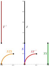
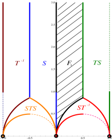
At this point it is convenient to discuss the domain of the lattices that play a role in the elliptic Jacobi functions and therefore in the solutions of the simple pendulum. As discussed in the appendix A, the quarter periods of a Jacobi elliptic function whose square modulus is in the interval $0<k^{2}\leq 1/2$, generate vertical lattices represented by a modular parameter of the form $\tau=iK_{c}/K$. The point $\tau=i$ is associated to the case where the rectangular lattice becomes square and corresponds to the value $k^{2}=1/2$. The set of all these lattices (black line in figure 3) is represented in the complex plane by the left vertical boundary of the region ${\cal F}_{1}$ (figure 5) since the quotient $K_{c}/K\in[1,\infty)$. Acting on these values of the modular parameter with the six group elements of $PSL(2,\mathbb{Z}/2\mathbb{Z})$ produce the whole set of values of the modular parameter (figure 3) that are consistent with the elliptic Jacobi functions. For example, acting with the $S$ group element of $\Gamma$ on the vertical line $\tau=iK_{c}/K$, generates the blue vertical line described mathematically by the set of modular parameters $\tau=iK/K_{c}$, with $K/K_{c}\in(0,1]$. It is clear that the set of six lines is a subset of the ${\cal F}_{2}$ fundamental region and constitutes the whole lattice domain of the elliptic Jacobi functions.

Figure 3: Figure shows the whole domain of values that the modular parameter $\tau$ can take for the Jacobi elliptic functions. This domain is a subset of the ${\cal F}_{2}$ fundamental region (figure 5). Black dots represent the values of the square modulus $k^{2}=1/2$, $1-k^{2}=1/2$, $1/k^{2}=2$, $1/(1-k^{2})=2$, $1-1/k^{2}=-1$ and $k^{2}/(k^{2}-1)=-1$.

In table 2 we give the numerical values (approximated) of the generators of the fundamental cell as well as the modular parameter for some values of the square modulus.

Modulus $k^{2}$	$\omega_{1}/4$	$\omega_{2}/4$	$\tau$
0	$\pi/2$	$i\cdot\infty$	$i\cdot\infty$
1/4	1.68575	$(2.15652)\,i$	$1.27926\,i$
1/2	1.85407	$(1.85407)\,i$	$i$
3/4	2.15652	$(1.68575)\,i$	$0.78170\,i$
1	$\infty$	$i\,\pi/2$	0
4/3	$2.87536+i\,2.24767$	$(2.24767)\,i$	$0.37929+i\,0.48521$
2	$3.70814(1\pm i)$	$(3.70814)\,i$	$\pm 0.5+i\,0.5$
4	$6.743-i\,8.62608$	$(8.62608)\,i$	$-0.62071+i\,0.48521$

Table 2: Approximated numerical values of the periods and the modular parameter for some real values of the modulus of the Jacobi elliptic functions. The values $k=0$ and $k=1$ correspond to limit situations where one of the two periods is lost. The value $k^{2}=1/2$ is known as a fixed point, it belongs both to the boundary of the regions ${\cal F}_{1}$ and $S$ of the fig. 5 and is represented by the black dot whose coordinates are $(0,i)$ in fig. 3. The value $k^{2}=2$ is degenerated in the sense it can be represented by two different types of fundamental cells, in one case the cell belongs to the boundary of the region $STS$ and in the another case it belongs to the boundary of $ST^{-1}$. The fundamental cell for some values of $k^{2}$ in this table are plotted in fig. 6.

As a conclusion, for every value of the parameter $0<k^{2}\leq 1/2$ there are six normal lattices related one to each other by transformations of the modular group. Therefore each solution of the simple pendulum with real time variable, showed in table 1, can be written in six different but equivalent ways, where each one of the six forms is in one to one correspondence with one of the six normal lattices. Their $S$-dual solutions (see table 1) which are functions of a pure imaginary time are just one of the six different ways in which solutions can be written.

IV.3 $STS$-duality

The form of the solutions for the simple pendulum expressed in table 1 does not coincide with the expressions given in section II, which by the way, are the standard form in which the solutions are commonly written in the literature. In order to reproduce the standard form it is necessary to introduce the $STS$ transformation (see appendix B). This transformation takes for instance a Jacobi function with modulus $0<k<1$ into a Jacobi function with modulus greater than one $1<1/k<\infty$. Taking the inverse transformation it is possible to take a Jacobi function with modulus $1<1/k$ into one with modulus $k<1$. Using the relations of the appendix B it is straightforward to obtain equations (78) which written in terms of $k_{E}$ instead of $k$ (remember than in this case $1<1/k=k_{E}$ $\Rightarrow$ $k=1/k_{E}<1$), lead to

$$k_{E}\,\mbox{sn}\left(x,k_{E}\right)=\mbox{sn}\left(k_{E}\,x,1/k_{E}\right),\hskip 14.22636ptk_{E}\,\mbox{cn}\left(x,k_{E}\right)=\mbox{dn}\left(k_{E}\,x,1/k_{E}\right),\hskip 14.22636pt\mbox{dn}\left(x,k_{E}\right)=\mbox{cn}\left(k_{E}\,x,1/k_{E}\right).$$ (34)

Inserting this relations in the circulating solutions of table 1 reproduce solutions (9) and (10).

What we have done is to use the $STS$-duality between lattices and transform two of them $kL^{*}$ and $ik_{c}L^{*}$ into $L^{*}$ and $iL^{*}$. Restricted to solutions with real time, two of the four type of solutions for which $k^{2}=k_{E}^{2}>1$, are transformed to solutions for which $k^{2}=1/k_{E}^{2}<1$. As we have discussed the domain of the solutions with real time variable are horizontal lines in the normal lattices $L^{*}$ and $iL^{*}$, thus in order to keep the four different types of solutions it is necessary to evaluate two different set of Jacobi functions (5) and (9) on the domain of each one of the two normal lattices $L^{*}$ and $iL^{*}$. It is clear that this is not the only way we can proceed, in fact we can transform the oscillatory solutions with $k<1$ into oscillatory solutions with modulus grater than 1. A similar analysis follows if we consider only solutions with imaginary time.

IV.4 A single normal lattice

It is natural to wonder about the minimum number of normal lattices needed to express all the solutions of the simple pendulum. Due to the duality symmetries between lattices this number is one. As an example, if we now use the $S$-duality to relate the normal horizontal lattice $iL^{*}$ to the normal vertical lattice $L^{*}$, the horizontal lines that compose the domain in the horizontal lattice becomes vertical lines in the vertical lattices, which means to consider solutions with imaginary time in $L^{*}$. Thus we can end up with only one normal lattice and in order to have the four different types of solutions, it is necessary to consider the whole domain of the lattice, i.e. both vertical lines (imaginary time) and horizontal lines (real time) and on each set of lines to consider two different solutions one oscillatory and one circulating. For completeness in table 3 we give the four type of solutions in terms of only one value of the modulus

Energy interval	Solution $\theta$
$k_{E}^{2}\in(0,1/2]$	2 $\arcsin[k$ sn$(x,k)]$
$k_{E}^{2}\in[1/2,1)$	2 $\arcsin[$dn$(ix-iK_{c}+K,k)]$
$k_{E}^{2}\in(1,2]$	$\pm$ 2 sgn[$(-ik/k_{c})$ cn$(ix/k_{c}-iK_{c}/k_{c},k)]\arcsin[(1/k_{c})$ dn$(ix/k_{c}-iK_{c}/k_{c},k)]$
$k_{E}^{2}\in[2,\infty)$	$\pm$ 2 sgn[cn$(x/k,k)]\arcsin$[sn$(x/k,k)]$

Table 3: Solutions to the simple pendulum problem written in a unique lattice of square modulus $0<k^{2}\leq 1/2$.

It is clear that we can express all the solutions also for the other five different functional forms of the square modulus.

V Final remarks

In this paper we have addressed the meaning of the fact that the complex domain of the solutions of the simple pendulum is not unique and in fact they are related by the $PSL(2,\mathbb{Z}/2\mathbb{Z})$ group, finding that the important issue for express the solutions is the relation between the values of the square modulus $k^{2}$ of the Jacobi elliptic functions, and the value of the total mechanical energy $k^{2}_{E}$ of the motion of the pendulum. Due to the symmetry we conclude that there are six different expressions of the square modulus that are related one to each other trough the six group elements of $PSL(2,\mathbb{Z}/2\mathbb{Z})$. These six group actions can be termed as duality-transformations and therefore we have six dual representations of $k^{2}$. As a consequence there are six different but equivalent ways in which we can write an specific pendulum solution, and abusing a little bit of the language we could say there are duality relations between solutions. This analysis teach us the lesson that we can restrict the domain of lattices to the ones whose modular parameter is in the pure imaginary interval $\tau\in i(1,\infty)$, or equivalently that we can express every solution of the simple pendulum either oscillatory or circulating with Jacobi elliptic functions whose value of the square modulus is in the interval $0<k^{2}\leq 1/2$ (see table 3).

It is well known that there are several physical systems in different areas of physics whose solutions are also given by elliptic functions, for instance in classical mechanics some examples are the spherical pendulum, the Duffing oscillator, etc., in Field Theory the Korteweg de Vries equation, the Ising model, etc., Brizard (2009); Petropoulos and Vanhove (2012). It would be very interesting to investigate on similar grounds to the ones followed here, the physical meaning of the symmetries of the elliptic functions in these systems.

Appendix A The modular group and its congruence subgroups

A.1 The modular group

The modular group $\Gamma$ is the group defined by the linear fractional transformations on the modular parameter $\tau\in\mathbb{C}$ (see for instance Du Val (1973); Lang (1973); Serre (1973); Lawden (1989); McKean and Moll (1999); Armitage and Eberlein (2006); Diamond and Shurman (2000) and references therein)

$$\tau\mapsto\Gamma(\tau)=\frac{a\tau+b}{c\tau+d},$$ (35)

where $a,b,c,d\in\mathbb{Z}$ satisfying $ad-bc=1$, and the group operation is function composition. These maps all transform the real axis of the $\tau$ plane (including the point at infinity) into itself, and rational values into rational values. The group has two generators defined by the transformations

$$S(\tau)\equiv-1/\tau,\hskip 14.22636pt\mbox{and}\hskip 14.22636ptT(\tau)\equiv 1+\tau.$$ (36)

The modular group is isomorphic to the projective special linear group $PSL(2,\mathbb{Z})$, which is the quotient of the 2-dimensional special linear group $SL(2,\mathbb{Z})$ by its center $\{\mathbb{I},-\mathbb{I}\}$. In other words, $PSL(2,\mathbb{Z})=SL(2,\mathbb{Z})/\mathbb{Z}_{2}$ consists of all matrices of the form

$$A=\left(\begin{matrix}a&b\\ c&d\end{matrix}\right),$$ (37)

with unit determinant, and pair of matrices $A$, $-A$, are considered to be identical. The group operation is multiplication of matrices and the generators accordingly with (36) are

$$S=\left(\begin{matrix}0&-1\\ 1&\,\,\,\,0\end{matrix}\right),\hskip 28.45274ptT=\left(\begin{matrix}1&1\\ 0&1\end{matrix}\right).$$ (38)

These group elements satisfy $S^{2}=(ST)^{3}=-\mathbb{I}\sim\mathbb{I}$ and $T^{n}=\left(\begin{matrix}1&n\\ 0&1\end{matrix}\right)$.

One important property of the modular group is that the upper half plane of $\mathbb{C}$, usually denoted as $\cal{H}$ and defined as ${\cal H}\equiv\{z\in\mathbb{C}:Im(z)>0\}$, can be generated by the elements of $PSL(2,\mathbb{Z})$ from a fundamental domain or region ${\cal F}$. Mathematically this region is the quotient space ${\cal F}={\cal H}/PSL(2,\mathbb{Z})$ and satisfies two properties: (i) ${\cal F}$ is a connected open subset of ${\cal H}$ such that no two points in ${\cal F}$ are related by a $\Gamma$ transformation (35) and (ii) for every point in ${\cal H}$ there is a group element $g\in\Gamma$ such that $g\tau\in{\cal F}$. There are many ways of constructing ${\cal F}$, and the most common one found in the literature is to take the set of all points $z$ in the open region $\{z:-1/2<\mbox{Re}(z)<1/2\cap|z|>1\}$, union “half” of its boundary, for instance, the one that includes the points: $z=-1/2+iy$ with $y\geq\sin(2\pi/3)$, and $|z|=1$ with $-1/2\leq$ Re$(z)\leq 0$ (see figure 4). It is assumed that the imaginary infinite is also included.

Figure 4: Tessellation of ${\cal H}$. The fundamental region ${\cal F}$ is represented by the shaded area and the heavy part of the boundary. This region is mapped to the whole upper plane $\mathbb{C}$ by the modular group $\Gamma$. The region can be viewed as a complete list of the inequivalent complex structures on the topological torus since conformal equivalence of tori is determined by the modular equivalence of their period ratios. In the figure we show some copies of the fundamental region obtained by application of some group elements of $PSL(2,\mathbb{Z})$.

Geometrically, $T$ represents a shift of ${\cal F}$ to the right by 1, while $S$ represents the inversion of ${\cal F}$ about the unit circle followed by reflection about the imaginary axis. As an example, the figure 4 represents the transformations of the fundamental region ${\cal F}$ by the elements of the group: $\{\mathbb{I},T,T^{-1},S,TS,T^{-1}S,ST,ST^{-1},ST^{-1}S,TST^{-1},STS,T^{-1}ST\}$ Serre (1973). Notice that these 12 elements are all the independent ones that we can construct as iterative products of $S$, $T$ and $T^{-1}$ without powers of any of them involved ($S^{-1}$ is simply $-S\sim S$ and therefore is not a different modular transformation). The other two transformations we can construct are not independent $TST=-ST^{-1}S$ and $T^{-1}ST^{-1}=STS$. Further products of the generators with these transformations give us the whole tessellation of the upper complex plane. In particular the orbit of the points Im$(z)\rightarrow\infty$ are the rational numbers $\mathbb{Q}$ and are called cusps.

A.2 Congruence subgroups

Relevant for our discussion are the congruence subgroups of level $N$ denoted as $\Gamma(N)$ (or $\Gamma_{N}$). They are defined as subgroups of the modular group $\Gamma$, which are obtained by imposing that the set of all modular transformations be congruent to the identity mod $N$

$$\Gamma(N)=\left\{\left(\begin{matrix}a&b\\ c&d\end{matrix}\right)\subset SL(2,\mathbb{Z}):\left(\begin{matrix}a&b\\ c&d\end{matrix}\right)=\left(\begin{matrix}1&0\\ 0&1\end{matrix}\right)\,(\mbox{mod}\,N)\right\}.$$ (39)

In this nomenclature the modular group $\Gamma$ is called the modular group of level 1 and denoted as $\Gamma(1)$ McKean and Moll (1999); Diamond and Shurman (2000). A relevant mathematical structure is the coset of the modular group with the congruence subgroups which are isomorphic to $PSL(2,\mathbb{Z}/N\mathbb{Z})$ Diamond and Shurman (2000)

$$\frac{SL(2,\mathbb{Z})}{\Gamma(N)}\rightarrow PSL(2,\mathbb{Z}/N\mathbb{Z}).$$ (40)

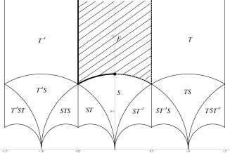
For the solutions of the simple pendulum the relevant congruence subgroup is the one of level 2: $\Gamma(2)$. It turns out that all the groups $PSL(2,\mathbb{Z}/N\mathbb{Z})$ are of finite order and in particular $PSL(2,\mathbb{Z}/2\mathbb{Z})$ is of order six. In table 4 we give explicitly the six elements of the coset and their corresponding form as group elements of $PSL(2,\mathbb{Z})$. Analogously to the case of the modular group, a fundamental cell for a subgroup $\Gamma(N)$ is a region ${\cal F}_{N}$ in the upper half plane that meets each orbit of $\Gamma(N)$ in a single point. Because $\Gamma(2)$ is of order six in $\Gamma$, a fundamental cell for $\Gamma(2)$ can be formed from the six copies of any fundamental cell ${\cal F}$ of $\Gamma$ produced by the action of the six elements. In figure 5 we show the fundamental region ${\cal F}_{2}$ of $\Gamma(2)$. This cell can be obtained from the region denoted as ${\cal F}_{1}$ which is a different fundamental region for $\Gamma$ as compared to the usual region ${\cal F}$ of the figure 4. ${\cal F}_{1}$ is obtained if ${\cal F}$ is replaced by its right half, plus inversion of its left half by the $S$ transformation. Thus ${\cal F}_{1}$ consists of the open region $\{z:0<\mbox{Re}(z)<1/2\cap\frac{z\bar{z}}{z+\bar{z}}>1\}$ and part of its boundary must be included. Geometrically $\frac{z\bar{z}}{z+\bar{z}}=1$ represents a unitary circle with center at $z=1$. A possible choice of the boundary includes the set of all points $\{z:z=iy$ with $y\geq 1\}$ union $\{z:\frac{z\bar{z}}{z+\bar{z}}=1$ with $0<$ Re$(z)\leq 1/2\}$. The full fundamental region ${\cal F}_{2}$ so produced is the part of the half-plane above the two circles of radius $1/2$ centered at $\pm 1/2$.

Figure 5: Fundamental cell ${\cal F}_{2}$ for $\Gamma(2)$. The heavy part of the figure is retained, the rest is not. In particular the cusps $-1$, $0$, $1$ and $i\infty$ are excluded.

As a complementary comment we mention that sometimes in the literature $\Gamma(2)$ appears under the name of modular group $\Lambda$. It turns out that the group is isomorphic to the symmetric group $S_{3}$, which is the group of all permutations of a three-element set and also to the dihedral group of order six (degree three) $D_{6}$, which represents, the group of symmetries (rotations and reflections) of the equilateral triangle.

A.3 Lattices

A lattice $L$ is an aggregate of complex numbers with two properties Du Val (1973): (i) is a group with respect to addition and (ii) the absolute magnitudes of the non-zero elements are bounded below. Because the Jacobi elliptic functions are meromorphic functions on $\mathbb{C}$, that are periodic in two directions: $f(z)=f(z+\omega_{1})=f(z+\omega_{2})$, we are interested in the so-called double lattices, consisting of all linear combinations with integer coefficients of two generating coefficients or primitive periods $\omega_{1},\omega_{2}\in\mathbb{C}$, whose ratio is imaginary

$$L(\omega_{1},\omega_{2})=\{n\omega_{1}+m\omega_{2}|n,m\in\mathbb{Z}\}\hskip 14.22636pt\mbox{such that}\hskip 14.22636ptf(z)=f(z+n\omega_{1}+m\omega_{2}),\hskip 14.22636pt\forall\,\,z\in\mathbb{C}.$$ (41)

The lattice points are the vertices of a pattern of parallelograms filling the whole plane, whose sides can be taken to be any pair of generators. The shapes of the lattices define equivalence classes. If $L(\omega_{1},\omega_{2})$ is any lattice, and the number $k\neq 0\in\mathbb{C}$, then $kL(\omega_{1},\omega_{2})$ denotes the aggregate of complex numbers $kz$ for all $z\in L(\omega_{1},\omega_{2})$ and it is also a lattice, which is said to be in the same equivalence class as $L(\omega_{1},\omega_{2})$. If $\bar{L}$ denotes the aggregate of complex numbers $\bar{z}$, $\forall$ $z\in L$; $\bar{L}$ is also a lattice. If $\bar{L}=L$, the lattice is called real. If the primitive periods can be chosen so that $\omega_{1}$ is real and $\omega_{2}$ pure imaginary, $L$ is called rectangular.

Rectangular lattices are real, and they are called horizontal or vertical, according as the longer sides of the rectangles are horizontal or vertical. The particular case in which both sides are equal is called the square lattice. Every lattice satisfies $L=-L$, and the only square lattice for which, $L=\alpha L$, with $\alpha\neq\pm 1$, is the lattice $iL$. If $L$ is a vertical rectangular lattice, $iL$ is a horizontal rectangular lattice and vice versa.

Associated to the lattice is the concept of residue classes. If $z$ is any complex variable, $z+L$ denotes the aggregate of values $z+\omega$ for all $\omega$ in the lattice $L$. This aggregate is called a residue class (mod $L$). The residue classes (mod $L$) form a continuous group under addition, defined in the way $(z+L)+(w+L)=(z+w)+L$. $L$ itself is a residue class (mod $L$), the zero element of the group. These residue classes allow to introduce the concept of fundamental region of $L$, consisting in a simply connected region of the complex plane which contains exactly one member of each residue class (mod $L$) . A fundamental region can be chosen in many ways, the simplest and usually the most convenient, is what is called either a unit cell, a fundamental cell or a fundamental parallelogram which is defined by all the points of the sides $\vec{\omega}_{1}$ and $\vec{\omega_{2}}$, including the vertex $\vec{0}$, but excluding the rest of the boundary and of course the whole interior points of the parallelogram. Mathematically the cell is given by the coset space $\mathbb{C}/L(\omega_{1},\omega_{2})$, where abusing of the notation, in this expression $L$ is considered as a residue class. Since the opposite sides of the fundamental cell must be identified, the coset space $\mathbb{C}/L(\omega_{1},\omega_{2})$ is homeomorphic to the torus $\mathbb{T}^{2}$. In other words, the pair $(\omega_{1},\omega_{2})$ defines a complex structure of $\mathbb{T}^{2}$ Nakahara (2003).

The shape of the lattice is determined by the modular parameter $\tau\equiv\omega_{2}/\omega_{1}$. It is important to note that, while a pair of primitive periods $\omega_{1}$, $\omega_{2}$, generates a lattice, a lattice does not have any unique pair of primitive periods, that is, many fundamental pairs (in fact, an infinite number) correspond to the same lattice. Specifically a change of generators $\omega_{1}$, $\omega_{2}$ to $\omega^{\prime}_{1}$ and $\omega^{\prime}_{2}$ of the form

$$\left(\begin{matrix}\omega^{\prime}_{2}\\ \omega^{\prime}_{1}\end{matrix}\right)=\left(\begin{matrix}a&b\\ c&d\end{matrix}\right)\left(\begin{matrix}\omega_{2}\\ \omega_{1}\end{matrix}\right),$$ (42)

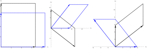
induces a mapping on the modular parameter $\tau$, belonging to the modular group. These maps are the link between the concepts of lattices, torus and modular group. As an example we discuss the mapping on $\tau$ induced by the generators (36). The generator $S$ interchanges the roles of the generators of the lattice $\omega_{1}\leftrightarrow\omega_{2}$ or equivalently it changes the longitude $l$ for the meridian $m$ of the torus and vice versa. The transformation $T$ generates a Dehn twist along the meridian which can be understood as follows Nakahara (2003). As a first step cut the torus along the meridian $m$, then take one of the lips of the cut and rotate it by $2\pi$ with the other lip kept fix and finally glue the lips together again.

Figure 6: Figure shows the fundamental cell for six different normal lattices. In the first plot the vertical cell corresponds to a value of the square modulus $k^{2}=1/4$ and belongs to a normal lattice of the type $L^{*}$. Under an $S$ transformation, the cell transforms to the horizontal one whose value of the square modulus is $k^{2}=3/4$ and belongs to a normal lattice $iL^{*}$. Analogously in the second and third plots, the fundamental cells in black belong to the lattices $kL^{*}$ and $ik_{c}L^{*}$ respectively, with values of the square modulus $k^{2}=4$ and $k^{2}=4/3$. The blue cells are obtained as their $S$-dual fundamental cells and have the values $k^{2}=-3$ and $k^{2}=-1/3$ and belong to normal lattices of the kind $ikL^{*}$ and $k_{c}L^{*}$ respectively. In every case, the continuous lines are included in the fundamental cell, whereas the dashed lines are not. The numerical values of the two generators $\omega_{1}$ and $\omega_{2}$ are given in table 2.

If the stationary values $e_{1}$, $e_{2}$ and $e_{3}$ are the roots of the cubic equation $4x^{3}-g_{2}x-g_{3}=0$, for any lattice $L$, with assigned generators $\omega_{1}$, $\omega_{2}$, we can define the scale constant $h$ by means of the relation: $h^{2}=e_{1}-e_{2}$, and the moduli as

$$k^{2}=\frac{e_{3}-e_{2}}{h^{2}},\hskip 28.45274ptk_{c}^{2}=\frac{e_{1}-e_{3}}{h^{2}}.$$ (43)

A lattice for which $h^{2}=1$ is called normal, and using the notation of Du Val (1973), we write it with a star $L^{*}$. Every lattice $L$ with assigned generators is similar to a unique normal lattice $L^{*}=hL$ with corresponding generators, since $e_{i}(hL)=h^{-2}e_{i}(L)$. For a given lattice shape with no assignments of generators, there are six normal lattices, as any of the six differences $e_{i}-e_{j}$ can be taken as $h^{2}$. If one of these is $L^{*}$, with modulus $k$, the others are $iL^{*}$, $kL^{*}$, $ikL^{*}$, $k_{c}L^{*}$ and $ik_{c}L^{*}$, with moduli $k_{c}$, $1/k$, $ik_{c}/k$, $ik/k_{c}$ and $1/k_{c}$ respectively, where $k^{2}+k_{c}^{2}=1$. These fall into three pairs which are of the same size, interchanged by a rotation of a right angle.

For the rectangular lattice shape, the six normal lattices are all real. Ordinarily $\omega_{1}$ is taken real and $\omega_{2}$ pure imaginary, so that $e_{1}>e_{3}>e_{2}$, and $0<k^{2}<1$, $0<k_{c}^{2}<1$, with $k^{2}<1/2<k_{c}^{2}$ if $L$ is vertical. We summarize the properties of the normal lattices in table 4

$\Gamma$	$PSL(2,\mathbb{Z})$	$PSL(2,\mathbb{Z}/2\mathbb{Z})$	Modulus	Quarter periods	Action on $k^{2}$	Normal lattice
$\tau$	$\pm\mathbb{I}$	$\pm\left(\begin{array}[]{cc}1&0\\ 0&1\end{array}\right)$	$k$	$K$, $iK_{c}$	$k^{2}\in(0,1/2]$	$L^{*}$
$-\frac{1}{\tau}$	$\pm S$	$\pm\left(\begin{array}[]{cc}0&-1\\ 1&\,\,\,\,0\end{array}\right)$	$k_{c}$	$K_{c}$, $iK$	$1-k^{2}\in[1/2,1)$	$iL^{*}$
$\frac{\tau}{1-\tau}$	$\pm STS$	$\mp\left(\begin{array}[]{cc}\,\,\,\,1&0\\ -1&1\end{array}\right)$	$\frac{1}{k}$	$k(K-iK_{c})$, $ikK_{c}$	$\frac{1}{k^{2}}\in[2,\infty)$	$kL^{*}$
$\frac{\tau-1}{\tau}$	$\pm TS$	$\pm\left(\begin{array}[]{cc}1&-1\\ 1&\,\,\,\,0\end{array}\right)$	$i\frac{k_{c}}{k}$	$kK_{c}$, $ik(K-iK_{c})$	$1-\frac{1}{k^{2}}\in(-\infty,-1]$	$ikL^{*}$
$\frac{1}{1-\tau}$	$\pm ST^{-1}$	$\mp\left(\begin{array}[]{cc}\,\,\,\,0&1\\ -1&1\end{array}\right)$	$\frac{1}{k_{c}}$	$k_{c}(K_{c}+iK)$, $ik_{c}K$	$\frac{1}{1-k^{2}}\in(1,2]$	$ik_{c}L^{*}$
$\tau-1$	$\pm T^{-1}$	$\pm\left(\begin{array}[]{cc}1&-1\\ 0&\,\,\,\,1\end{array}\right)$	$i\frac{k}{k_{c}}$	$k_{c}K$, $ik_{c}(K_{c}+iK)$	$\frac{k^{2}}{k^{2}-1}\in[-1,0)$	$k_{c}L^{*}$

Table 4: Main characteristics of the six order $PSL(2,\mathbb{Z}/2\mathbb{Z})$ group and its relation to the six normal lattices.

Appendix B Jacobi elliptic functions

In the previous appendix we reviewed the action of the modular group on the modular parameter. In this appendix we want to specialize that discussion to the case of the elliptic Jacobi functions. In particular we are interested in the relation between the six dimensional group $PSL(2,\mathbb{Z}/2\mathbb{Z})$ and what is called transformations of the elliptic Jacobi functions. There are three transformations that are exposed often in the literature, the Jacobi’s imaginary transformation, the Jacobi’s imaginary modulus transformation and the Jacobi’s real transformation. These are transformations that relate the Jacobi elliptic functions with different value of the square modulus $k^{2}$. Behind these transformations is the property that the modulus of the Jacobi functions can be defined in the real line $k^{2}\in\mathbb{R}$ with exception of the points $z=-1,0,1$, and it can be divided in six intervals

$$k^{2}\in(-\infty,-1]\,\cup[-1,0)\cup(0,1/2]\cup[1/2,1)\cup(1,2]\cup[2,\infty).$$

These six intervals are in one to one relation to the column Action on $k^{2}$ in table (4), if we consider that the modulus in the fundamental region ${\cal F}_{1}$ of $PSL(2,\mathbb{Z})$ takes values in the interval $0\leq k^{2}\leq 1/2$. In the following we summarize some of the properties of the Jacobi elliptic functions that are useful throughout the paper.

B.1 Jacobi elliptic functions with modulus $0<k^{2}<1$

The Jacobi elliptic functions are meromorphic functions in ${\mathbb{C}}$, that have a fundamental real period and a fundamental complex period, i.e., they are doubly periodic. The periods are determined by the value of the square modulus and in the following we assume that $0<k^{2}<1$.

The primitive real period of the three basic functions can be inferred from the following relations which are dictated by the addition formulas for the Jacobi functions Whittaker and Watson (1927); Du Val (1973); Lang (1973); Lawden (1989); McKean and Moll (1999); Armitage and Eberlein (2006)

$$\mbox{sn}(z+K,k)=\frac{\mbox{cn}(z,k)}{\mbox{dn}(z,k)},\hskip 14.22636pt\mbox{cn}(z+K,k)=-k_{c}\frac{\mbox{sn}(z,k)}{\mbox{dn}(z,k)},\hskip 14.22636pt\mbox{dn}(z+K,k)=k_{c}\frac{1}{\mbox{dn}(z,k)},$$ (44)

where the quarter-period $K$ is defined as function of the square modulus $k^{2}$ as

$$K\equiv\int_{0}^{1}\frac{du}{\sqrt{(1-u^{2})(1-k^{2}u^{2})}}.$$ (45)

In particular we obtain the values sn$(K,k)=1$, cn$(K,k)=0$ and dn$(K,k)=k_{c}$, from the ones sn$(0,k)=0$, cn$(0,k)=1$ and dn$(0,k)=1$. Iteration of relations (44) leads to

$$\mbox{sn}(z+2K,k)=-\mbox{sn}(z,k),\hskip 14.22636pt\mbox{cn}(z+2K,k)=-\mbox{cn}(z,k),\hskip 14.22636pt\mbox{dn}(z+2K,k)=\mbox{dn}(z,k).$$ (46)

The last relation is telling that the function dn($z,k$) has real period $2K$. A further $2K$ iteration will tell us that the other two Jacobi elliptic functions (sn($z,k$) and cn($z,k$)) have primitive real period $4K$. Regarding the complex period, we have the relations

$$\mbox{sn}(z+iK_{c},k)=\frac{1}{k}\frac{1}{\mbox{sn}(z,k)},\hskip 14.22636pt\mbox{cn}(z+iK_{c},k)=-i\frac{1}{k}\frac{\mbox{dn}(z,k)}{\mbox{sn}(z,k)},\hskip 14.22636pt\mbox{dn}(z+iK_{c},k)=-i\frac{\mbox{cn}(z,k)}{\mbox{sn}(z,k)},$$ (47)

where $K_{c}$ is defined as function of the so-called complementary modulus $k_{c}^{2}\equiv 1-k^{2}$ in the form

$$K_{c}\equiv\int_{0}^{1}\frac{du}{\sqrt{(1-u^{2})(1-k_{c}^{2}u^{2})}}.$$ (48)

Iterating these relations once leads to

$$\mbox{sn}(z+2iK_{c},k)=\mbox{sn}(z,k),\hskip 14.22636pt\mbox{cn}(z+2iK_{c},k)=-\mbox{cn}(z,k),\hskip 14.22636pt\mbox{dn}(z+2iK_{c},k)=-\mbox{dn}(z,k).$$ (49)

The first relation is telling us that the elliptic function sn($z,k$) has a pure imaginary primitive period $2iK_{c}$. A further $2iK_{c}$ iteration leads to the conclusion that the elliptic function dn($z,k$) has a pure imaginary primitive period $4iK_{c}$ whereas the elliptic function cn($z,k$) has a fundamental period $4iK_{c}$. In the latter case notice that combining the second relation of (46) and the second relation of (49) leads to the result cn$(z+2K+2iK_{c},k)=\mbox{cn}(z,k)$ concluding that this elliptic function has a primitive complex period $2K+2iK_{c}$. In summary, the primitive periods of the three basic Jacobi functions are

$$\mbox{sn}(z,k) = \mbox{sn}(z+4K,k)=\mbox{sn}(z+2iK_{c},k),$$ (50)

$$\mbox{cn}(z,k) = \mbox{cn}(z+4K,k)=\mbox{cn}(z+2K+2iK_{c},k),$$ (51)

$$\mbox{dn}(z,k) = \mbox{dn}(z+2K,k)=\mbox{dn}(z+4iK_{c},k).$$ (52)

Because these periods do not coincide one looks for two common periods in order to define a common fundamental cell for the three functions. These fundamental periods are $4K$ and $4iK_{c}$, they are not primitive because linear combinations of them does not give origin for instance to the primitive period $2K+2iK_{c}$ of cn$(z,k)$. The fundamental cell for the Jacobi elliptic functions is, therefore, the parallelogram with vertices $(0,4K,4iK_{c},4K+4iK_{c})$, and the modular parameter $\tau$ turns out to be

$$\tau\equiv\frac{iK_{c}}{K}.$$ (53)

Given this definition of the modular parameter we see that not every point of ${\cal F}_{1}$ corresponds to a modulus $k^{2}$ of the Jacobi functions but only the values on the vertical boundary $\tau\in[i,i\infty)$, being the point $\tau=i$ the one that corresponds to $k^{2}=1/2$, since in this case $K=K_{c}$ and therefore the corresponding normal lattice is squared. The rest of points on the vertical boundary corresponds to vertical normal lattices because $K<K_{c}$ and all of them have a value of the square modulus $0<k^{2}<1/2$. By acting the five group elements of $PSL(2,\mathbb{Z}/2\mathbb{Z})$ different from the identity to the modular parameter values on the vertical boundary of ${\cal F}_{1}$, we can generate the whole set of possible values of $\tau$ and therefore the whole set of possible values of the square modulus $k^{2}$ of the Jacobi functions (see figure 3).

Derivatives of the basic functions, which are necessary to obtain the angular velocities are

$$\frac{d}{dz}\mbox{sn}(z,k)=\mbox{cn}(z,k)\,\mbox{dn}(z,k),\hskip 8.5359pt\frac{d}{dz}\mbox{cn}(z,k)=-\mbox{sn}(z,k)\,\mbox{dn}(z,k),\hskip 8.5359pt\frac{d}{dz}\mbox{dn}(z,k)=-k^{2}\mbox{sn}(z,k)\,\mbox{cn}(z,k).$$ (54)

B.2 Jacobi’s imaginary transformation

The transformation induced by the generator $S(\tau)$ of the modular group on the Jacobi functions with modulus $k$, is known as the Jacobi’s imaginary transformation. In this case the modulus and the complementary modulus exchange with each other

$$k\mapsto k_{c}\hskip 14.22636pt\mbox{and}\hskip 14.22636ptk_{c}\mapsto k\hskip 14.22636pt\Rightarrow\hskip 14.22636ptK\mapsto K_{c}\hskip 14.22636pt\mbox{and}\hskip 14.22636ptK_{c}\mapsto K.$$ (55)

Applying this transformation on the vertical boundary of ${\cal F}_{1}$, generates both the transformed pure imaginary modular parameter and the transformed modulus which belong to the intervals $\tau\in(0,i]$ and $1/2\leq k_{c}^{2}=1-k^{2}<1$, respectively. The Jacobi functions itself transform as

$$\mbox{sn}(z,k_{c})=-i\,\mbox{sc}(iz,k),\hskip 14.22636pt\mbox{cn}(z,k_{c})=\mbox{nc}(iz,k),\hskip 14.22636pt\mbox{dn}(z,k_{c})=\mbox{dc}(iz,k).$$ (56)

This is the mathematical property behind the analysis made by Appell to deal with solutions of imaginary time. These transformations are used very often to change a pure imaginary argument $ix$ to one real $x$, obtaining

$$\mbox{sn}(ix,k)=i\,\mbox{sc}(x,k_{c}),\hskip 14.22636pt\mbox{cn}(ix,k)=\mbox{nc}(x,k_{c}),\hskip 14.22636pt\mbox{dn}(ix,k)=\mbox{dc}(x,k_{c}).$$ (57)

From a geometrical point of view the normal vertical cell $L^{*}$ with vertices $(0,4K,4iK_{c},4K+4iK_{c})$ changes to the normal horizontal cell $iL^{*}$ with vertices $(0,4K_{c},4iK,4K_{c}+4iK)$ and the corresponding torus is obtained from the original one by an interchange of their respective meridians and longitudes. The rest of properties of the functions are obtained from the ones in (section B.1) by setting $z=ix$ and implementing in the expressions the interchanges $k\leftrightarrow k_{c}$ and $K\leftrightarrow K_{c}$.

B.3 Jacobi’s imaginary modulus transformation

The transformation induced by the generator $T(\tau)$ of the modular group on the Jacobi functions, is known as the imaginary modulus transformation, because under this transformation the modulus change as

$$k\mapsto i\frac{k}{k_{c}},\hskip 14.22636pt\mbox{and}\hskip 14.22636ptk_{c}\mapsto\frac{1}{k_{c}},$$ (58)

which induces a change in the quarter periods of the form

$$K\mapsto k_{c}K,\hskip 14.22636pt\mbox{and}\hskip 14.22636ptK_{c}\mapsto k_{c}(K_{c}-iK).$$ (59)

Applying this transformation to the vertical boundary of ${\cal F}_{1}$, generates the transformed modular parameter which lies on the vertical line $\tau\in[1+i,1+i\infty)$ and the transformed square modulus which takes values in the interval $-1\leq\frac{k^{2}}{k^{2}-1}<0$. The transformation rule for the Jacobi functions itself are

$$\mbox{sn}(z,ik/k_{c})=k_{c}\,\mbox{sd}(z/k_{c},k),\hskip 14.22636pt\mbox{cn}(z,ik/k_{c})=\mbox{cd}(z/k_{c},k),\hskip 14.22636pt\mbox{dn}(z,ik/k_{c})=\mbox{nd}(z/k_{c},k).$$ (60)

It is clear that this transformation allows us to define the Jacobi functions with an imaginary modulus in terms of the Jacobi functions with real modulus. Replacing $z\mapsto k_{c}z$, we can express these transformations in its more usual form

$$\mbox{sn}(k_{c}z,ik/k_{c})=k_{c}\,\mbox{sd}(z,k),\hskip 14.22636pt\mbox{cn}(k_{c}z,ik/k_{c})=\mbox{cd}(z,k),\hskip 14.22636pt\mbox{dn}(k_{c}z,ik/k_{c})=\mbox{nd}(z,k).$$ (61)

From a geometrical point of view the fundamental vertical cell with vertices $(0,4K,4iK_{c},4K+4iK_{c})$ changes to the fundamental cell with vertices $(0,4k_{c}K,4k_{c}K+4ik_{c}K,8k_{c}K+4ik_{c}K_{c})$ and the corresponding torus is changed by a Dehn twist. Notice that by applying further the transformation $S$ to these expressions, we obtain a fundamental cell where the quarter periods (59) are interchange among them an the value of the square modulus is defined in the interval, $1<\frac{1}{1-k^{2}}\leq 2$, since the modulus (58) also interchanges one to the another.

The elliptic Jacobi functions with negative square modulus satisfy analogous relations to the Jacobi functions with modulus $0<k^{2}<1$, these are obtained from equations (60) and the corresponding relation of the Jacobi functions with $0<k^{2}<1$. For instance, the equations analogous to (13) and (15) are

$$\mbox{sn}^{2}(z,ik/k_{c})+\mbox{cn}^{2}(z,ik/k_{c})=1,\hskip 8.5359pt\mbox{and}\hskip 8.5359pt-\frac{k^{2}}{k_{c}^{2}}\mbox{sn}^{2}(z,ik/k_{c})+\mbox{dn}^{2}(z,ik/k_{c})=1.$$ (62)

Proceeding in a similar way it is possible to obtain the equations analogous to (44), these are

$$\mbox{sn}(z+K,ik/k_{c})=\frac{\mbox{cn}(z,ik/k_{c})}{\mbox{dn}(k_{c}z,ik/k_{c})},\hskip 2.84544pt\mbox{cn}(z+K,ik/k_{c})=-\frac{1}{k_{c}}\frac{\mbox{sn}(z,ik/k_{c})}{\mbox{dn}(k_{c}z,ik/k_{c})},\hskip 2.84544pt\mbox{dn}(z+K,ik/k_{c})=\frac{1}{k_{c}}\frac{1}{\mbox{dn}(z,ik/k_{c})},$$ (63)

which iterating once lead to the relations

$$\mbox{sn}(z+2K,ik/k_{c})=-\mbox{sn}(z,ik/k_{c}),\hskip 5.69046pt\mbox{cn}(z+2K,ik/k_{c})=-\mbox{cn}(z,ik/k_{c}),\hskip 5.69046pt\mbox{dn}(z+2K,ik/k_{c})=\mbox{dn}(z,ik/k_{c}).$$ (64)

The third relation is telling us that the function dn($z,ik/k_{c}$) has a fundamental period $2K$. A further $2K$ iteration leads to the conclusion that the other two Jacobi functions have a fundamental period of $4K$. Regarding the imaginary period, the equations analogous to (47) are

$$\mbox{sn}(z+iK_{c},ik/k_{c}) = i\frac{k_{c}}{k}\frac{\mbox{dn}(z,ik/k_{c})}{\mbox{cn}(k_{c}z,ik/k_{c})},$$ (65)

$$\mbox{cn}(z+iK_{c},ik/k_{c}) = \frac{1}{k}\frac{1}{\mbox{cn}(z,ik/k_{c})},$$ (66)

$$\mbox{dn}(z+iK_{c},ik/k_{c}) = i\frac{1}{k_{c}}\frac{\mbox{sn}(z,ik/k_{c})}{\mbox{cn}(k_{c}z,ik/k_{c})},$$ (67)

which after an iteration lead to

$$\mbox{sn}(z+2iK_{c},ik/k_{c})=-\mbox{sn}(z,ik/k_{c}),\hskip 2.84544pt\mbox{cn}(z+2iK_{c},ik/k_{c})=\mbox{cn}(z,ik/k_{c}),\hskip 2.84544pt\mbox{dn}(z+2iK_{c},ik/k_{c})=-\mbox{dn}(z,ik/k_{c}).$$ (68)

These relations indicate that the function cn$(z,ik/k_{c})$ has fundamental imaginary period $2iK_{c}$, whereas the other two Jacobi functions have $4iK_{c}$. In summary, the primitive periods of the three basic Jacobi functions are

$$\mbox{sn}(z,ik/k_{c}) = \mbox{sn}(z+4K,ik/k_{c})=\mbox{sn}(z+2K+2iK_{c},ik/k_{c}),$$ (69)

$$\mbox{cn}(z,ik/k_{c}) = \mbox{cn}(z+4K,ik/k_{c})=\mbox{cn}(z+2iK_{c},ik/k_{c}),$$ (70)

$$\mbox{dn}(z,ik/k_{c}) = \mbox{dn}(z+2K,ik/k_{c})=\mbox{dn}(z+4iK_{c},ik/k_{c}).$$ (71)

It is straightforward to verify that in this case the derivatives of the fundamental relations that follows from (54) are

$$\frac{d}{dz}\mbox{sn}(z,ik/k_{c})=\mbox{cn}(z,ik/k_{c})\,\mbox{dn}(z,ik/k_{c}),\hskip 8.5359pt\frac{d}{dz}\mbox{cn}(z,ik/k_{c})=-\mbox{sn}(z,ik/k_{c})\,\mbox{dn}(z,ik/k_{c}),$$ (72)

and

$$\frac{d}{dz}\mbox{dn}(z,ik/k_{c})=\frac{k^{2}}{k_{c}^{2}}\mbox{sn}(z,ik/k_{c})\,\mbox{cn}(z,ik/k_{c}).$$ (73)

B.4 Jacobi’s real transformation

In the literature of the elliptic functions, the transformation generated by the element $STS$ of the modular group

$$\tau_{I}=\frac{\tau}{1-\tau},$$ (74)

which can be obtained as a composition of the following three transformations

$$\tau_{I}=-\frac{1}{\tau_{2}},\hskip 28.45274pt\tau_{2}=1+\tau_{1},\hskip 28.45274pt\mbox{and}\hskip 28.45274pt\tau_{1}=-\frac{1}{\tau},$$ (75)

generates the so-called Jacobi’s real transformation. Under it, the modulus of the elliptic functions change as

$$k\mapsto\frac{1}{k},\hskip 14.22636pt\mbox{and}\hskip 14.22636ptk_{c}\mapsto i\frac{k_{c}}{k},$$ (76)

whereas the quarter periods transform as

$$K\mapsto k(K-iK_{c}),\hskip 14.22636pt\mbox{and}\hskip 14.22636ptK_{c}\mapsto kK_{c}.$$ (77)

Applying this transformation to the vertical boundary of ${\cal F}_{1}$, generates the transformed modular parameter which lies on the line $\tau=-\frac{y^{2}}{1+y^{2}}+i\frac{y}{1+y^{2}}$, with $y$ in the interval $y\in[1,\infty)$ and the transformed square modulus which takes values in the interval $2\leq 1/k^{2}<\infty$. The transformation rules for the Jacobi functions itself are

$$\mbox{sn}(z,1/k)=k\,\mbox{sn}(z/k,k),\hskip 14.22636pt\mbox{cn}(z,1/k)=\mbox{dn}(z/k,k),\hskip 14.22636pt\mbox{dn}(z,1/k)=\mbox{cn}(z/k,k).$$ (78)

This transformations allows us to define the Jacobi elliptic functions with square modulus greater than two in terms of Jacobi functions with modulus $0<k^{2}\leq 1/2$. Replacing $z\mapsto kz$, allows to express these transformations in its more usual form

$$\mbox{sn}(kz,1/k)=k\,\mbox{sn}(z,k),\hskip 14.22636pt\mbox{cn}(kz,1/k)=\mbox{dn}(z,k),\hskip 14.22636pt\mbox{dn}(kz,1/k)=\mbox{cn}(z,k).$$ (79)

A further application of the group transformation $S$ to these expressions leads to the interchange of the modulus (76) and to the interchange of the quarter periods (77). In this case the square modulus of the Jacobi functions is defined in the interval $-\infty<1-1/k^{2}\leq-1$.

As in the previous cases it is possible to obtain the fundamental periods of the three different basic Jacobi elliptic functions, since the arguments as before, we just list the equations. For the real period we have

$$\mbox{sn}(z+K,1/k)=k\,\frac{\mbox{dn}(z,1/k)}{\mbox{cn}(z,1/k)},\hskip 8.5359pt\mbox{cn}(z+K,1/k)=k_{c}\,\frac{1}{\mbox{cn}(z,1/k)},\hskip 8.5359pt\mbox{dn}(z+K,1/k)=-\frac{k_{c}}{k}\,\frac{\mbox{sn}(z,1/k)}{\mbox{cn}(z,1/k)},$$ (80)

and iterating we get

$$\mbox{sn}(z+2K,1/k)=-\mbox{sn}(z,1/k),\hskip 8.5359pt\mbox{cn}(z+2K,1/k)=\mbox{cn}(z,1/k),\hskip 8.5359pt\mbox{dn}(z+2K,1/k)=-\mbox{dn}(z,1/k).$$ (81)

As for the imaginary period

$$\mbox{sn}(z+iK_{c},1/k)=\frac{k}{\mbox{sn}(z,1/k)},\hskip 2.84544pt\mbox{cn}(z+iK_{c},1/k)=-ik\frac{{\mbox{dn}(z,1/k)}}{\mbox{sn}(z,1/k)},\hskip 2.84544pt\mbox{dn}(z+iK_{c},1/k)=-i\frac{\mbox{cn}(z,1/k)}{\mbox{sn}(z,1/k)},$$ (82)

and after an iteration

$$\mbox{sn}(z+2iK_{c},1/k)=\mbox{sn}(z,1/k),\hskip 2.84544pt\mbox{cn}(z+2iK_{c},1/k)=-\mbox{cn}(z,1/k),\hskip 2.84544pt\mbox{dn}(z+2iK_{c},1/k)=-\mbox{dn}(z,1/k).$$ (83)

In summary, the primitive periods of the three basic Jacobi functions are

$$\mbox{sn}(z,1/k) = \mbox{sn}(z+4K,1/k)=\mbox{sn}(z+2iK_{c},1/k),$$ (84)

$$\mbox{cn}(z,1/k) = \mbox{cn}(z+2K,1/k)=\mbox{cn}(z+4iK_{c},1/k),$$ (85)

$$\mbox{dn}(z,1/k) = \mbox{dn}(z+4K,1/k)=\mbox{dn}(z+2K+2iK_{c},1/k).$$ (86)

Finally, the equations analogous to (13) and (15) are

$$\mbox{sn}^{2}(z,1/k)+\mbox{cn}^{2}(z,1/k)=1,\hskip 8.5359pt\mbox{and}\hskip 8.5359pt\frac{1}{k^{2}}\mbox{sn}^{2}(z,1/k)+\mbox{dn}^{2}(z,1/k)=1.$$ (87)

whereas the derivatives of the basic functions are

$$\frac{d}{dz}\mbox{sn}(z,1/k)=\mbox{cn}(z,1/k)\,\mbox{dn}(z,1/k),\hskip 8.5359pt\frac{d}{dz}\mbox{cn}(z,1/k)=-\mbox{sn}(z,1/k)\,\mbox{dn}(z,1/k),$$ (88)

and

$$\frac{d}{dz}\mbox{dn}(z,1/k)=-\frac{1}{k^{2}}\mbox{sn}(z,1/k)\,\mbox{cn}(z,1/k).$$ (89)