Matter-wave soliton interferometer based on a nonlinear splitter

Abstract

We elaborate a model of the interferometer which, unlike previously studied ones, uses a local ($\delta$-functional) nonlinear repulsive potential, embedded into a harmonic-oscillator trapping potential, as the splitter for the incident soliton. An estimate demonstrates that this setting may be implemented by means of the localized Feshbach resonance controlled by a focused laser beam. The same system may be realized as a nonlinear waveguide in optics. Subsequent analysis produces an exact solution for scattering of a plane wave in the linear medium on the $\delta$-functional nonlinear repulsive potential, and an approximate solution for splitting of the incident soliton when the ambient medium is nonlinear. The most essential result, obtained by means of systematic simulations, is that the use of the nonlinear splitter provides the sensitivity of the soliton-based interferometer to the target, inserted into one of its arms, which is much higher than the sensitivity provided by the usual linear splitter.

I Introduction and the model

Matter-wave solitons are self-trapped modes in Bose gases with attractive interactions between atoms, which have been created in Bose-Einstein condensates (BECs) of ⁷Li Li and ⁸⁵Rb Rb ; reflection . Available experimental methods make it possible to efficiently steer the motion of solitons in matter-wave conduits, and study various dynamical phenomena, such as reflection of solitons from potential barriers reflection and collisions between solitons collision .

In addition to the obvious significance to fundamental studies, the solitons may find an important application to the design of matter-wave interferometers. Soliton-based interferometric schemes have been elaborated in many theoretical works interf-theory -Helm , and recently implemented in the experiment interf-exp . The main element of the interferometer is a narrow potential barrier, which provides for splitting of an incident soliton into two matter-wave pulses, that move apart in the harmonic-oscillator (HO) trapping potential into which the splitter is embedded, and return back, to collide and recombine on the splitter, as shown schematically in Fig. 1.

Figure 1: (a) The scheme of the soliton-based interferometer, with the initial soliton trapped in the HO potential and the splitting barrier installed at the center. The arrow indicates the direction of motion of the soliton. (b) A sketch of the operation of the interferometer, shown by means of the spatiotemporal evolution of the density: splitting of the incident soliton, followed by recombination of the secondary pulses (incomplete, in the general case), after the collision between them.

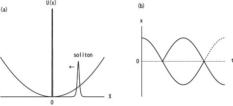
The interferometric effect is produced by placing a target in one arm of the interferometer (on the left- or right-hand side of the splitter), which affects the outcome of the secondary collision by shifting the phase of the pulse passing the target. The elaboration of this scheme makes it necessary to study in detail collisions of the pulses with the potential barrier, including such aspects as the deviation from one-dimensionality Cuevas , finite width of the barrier wide-rectangular , quantum effects beyond the limits of the mean-field theory quantum ; Helm ; quantum2 , collisions of two-component solitons 2comp-collision , etc. For the overall operation of the interferometer, a crucial factor is the phase stability of the colliding pulses phase-control ; collision , as the relative phase of the pulses determines the outcome of the collision. In this respect, the use of the solitons offers a potential advantage, as its collective phase degree of freedom is canonically conjugate to its norm (the same is true for quantum states squeeze ), hence for heavy solitons random phase fluctuations may be efficiently suppressed by the large value of the norm.

The main objective of the present work is to elaborate the soliton-based interferometric scheme which uses a nonlinear potential barrier (splitter), instead of the linear repulsive defect studied in the previous works. Assuming that the tight transverse confinement is provided by an isotropic HO potential with frequency $\Omega_{\perp}$, the corresponding mean-field wave function is looked for, as usual, in the factorized form BEC :

$$\Psi\left(\rho,X,T\right)=\frac{1}{\sqrt{\pi}a_{\perp}}\exp\left(-i\hbar\Omega_{\perp}T-\frac{\rho^{2}}{2a_{\perp}^{2}}\right)\Phi\left(X,T\right),~{}a_{\perp}^{2}=\frac{\hbar}{m\Omega_{\perp}},$$ (1)

where $\rho$ and $X$ are, respectively, the transverse-radial and longitudinal coordinates, $T$ is time, and $m$ the atomic mass. The ensuing scaled form of the one-dimensional (1D) Gross-Pitaevskii equation (GPE), which includes the barrier combining linear and nonlinear localized repulsive potentials, with respective strengths $\varepsilon_{0}>0$ and $\varepsilon_{2}>0$, as well as the longitudinal HO potential with strength $\Omega^{2}$, is

$$i\frac{\partial\phi}{\partial t}=\left[-\frac{1}{2}\frac{\partial^{2}}{\partial x^{2}}-g|\phi|^{2}+\frac{1}{2}\Omega^{2}x^{2}+\varepsilon_{0}\delta(x)+\varepsilon_{2}\delta(x)|\phi|^{2}\right]\phi,$$ (2)

where the strength of the background self-attraction is set to be $g=1$, unless $g=0$ in the linearized model, and $\delta(x)$ is the Dirac’s delta function. In numerical simulations reported below, it is replaced by a rectangular potential tower of width $\Delta x$ and height $1/\Delta x$, centered at $x=0$. The relation between the variables measured in physical units and their scaled counterparts is

$$X=X_{0}x,~{}T=\left(mX_{0}^{2}/\hbar\right)t,~{}\Phi=a_{\perp}\left(X_{0}\sqrt{\left|2\left(a_{s}\right)_{\mathrm{backgr}}\right|}\right)^{-1}\phi,$$ (3)

where $X_{0}$ is a characteristic scale of the longitudinal coordinate, and $\left(a_{s}\right)_{\mathrm{backgr}}<0$ is the scattering lengths of atomic collisions far from the barrier. Further, the frequency of the HO potential, measured in physical units, is $\omega=\left(\hbar/mX_{0}^{2}\right)\Omega$, the linear potential barrier is $\left(\hbar^{2}/mX_{0}\right)\varepsilon_{0}\delta(X)$, and the nonlinear barrier is defined, in terms of the full underlying GPE, as $\left(4\pi\hbar^{2}/m\right)X_{0}^{2}\varepsilon_{2}\delta(X)\left|\Psi\right|^{2}$.

The Hamiltonian (energy) corresponding to Eq. (2) is

$$E=\frac{1}{2}\int_{-\infty}^{+\infty}\left(\left|\frac{\partial\phi}{\partial x}\right|^{2}-g\left|\phi\right|^{4}+\Omega^{2}x^{2}\left|\phi\right|^{2}\right)dx$$

$$+\varepsilon_{0}\left|\phi(x=0)\right|^{2}+\frac{1}{2}\varepsilon_{2}\delta(x)\left|\phi(x=0)\right|^{4}$$ (4)

The number of atoms in the condensate, given by the norm of wave function (1) in physical units, is

$$N_{\mathrm{at}}=2\pi\int_{0}^{\infty}\rho d\rho\int_{-\infty}^{+\infty}dX~{}\left|\Psi\left(\rho,X\right)\right|^{2}\equiv\pi a_{\perp}^{2}\int_{-\infty}^{+\infty}\left|\Phi(x)\right|^{2}dX.$$ (5)

It is proportional to the norm of the scaled 1D wave function,

$$N=\int_{-\infty}^{+\infty}\left|\phi(x)\right|^{2}dx.$$ (6)

Indeed, it follows from Eq. (3) that

$$N_{\mathrm{at}}=a_{\perp}^{2}\left(2X_{0}\left|\left(a_{s}\right)_{\mathrm{backgr}}\right|\right)^{-1}N.$$ (7)

Estimates for typical values of physical parameters, including $N_{\mathrm{at}}$, which are relevant in the present context, are given below.

It is worthy to note that, for a sufficiently dense atomic gas, the factorization procedure leads to a deviation of the effective 1D nonlinearity from the simple cubic term 1D3D . The consideration of the nonlinear barrier combined with the more sophisticated background nonlinearity is an interesting issue too, which is left beyond the framework of the present work.

We will chiefly consider the model with the fully nonlinear potential barrier, setting $\varepsilon_{0}=0$ in Eq. (2). Recently, soliton dynamics in systems with spatially modulated nonlinearity has drawn much attention, as it opens new possibilities for controlling outcomes of the evolution of solitons by means of their amplitude, which is proportional to $N_{\mathrm{at}}$, see review RMP and references therein. A still more recent use of nonlinear potential barriers, of the same type as introduced in Eq. (2), was proposed in Ref. students in a model of a pumped laser cavity, where nonlinear barriers confined intra-cavity solitons, but allowed the release of small-amplitude radiation, thus stabilizing the trapped soliton modes students . In optics, strong local change of the nonlinearity may be induced by doping the respective small-area region by atoms providing resonant two-photon interaction with the electromagnetic wave Kip . In this connection, it is worthy to note that GPE (2) may also be realized, in terms of optics, as the nonlinear Schrödinger equation for the spatial-domain propagation in a planar waveguide, with transverse coordinate $x$, and $t$ replaced by the appropriately scaled propagation distance, $z$. In that case, the trapping potential defines the guiding channel, which is split into two by the $\delta$-functional terms $\sim\varepsilon_{0,2}$ NatPhot .

For the atomic BEC, the localized barrier can be created by means of the optically-controlled Feshbach resonance (FR) Feshbach-optical ; Tom ; Nicholson , that reverses the intrinsic BEC nonlinearity from uniformly attractive to strongly repulsive in a narrow region of width $\Delta x$, onto which the control laser beam is focused. It is relevant to estimate physical parameters which will make the creation of such a nonlinear barrier possible. Far from the barrier, the free soliton with amplitude $A$, moving at velocity $v$, is given by the commonly known solution of Eq. (2) with $g=1$ and $\Omega=0$:

$$\phi=A~{}\mathrm{sech}\left(x-\xi(t)\right)\exp\left(\frac{i}{2}\left(A^{2}-v^{2}\right)t\right),~{}v=\frac{d\xi}{dt}.$$ (8)

The scaled norm and energy of the free soliton are given by Eqs. (6) and (4) (dropping terms $\sim\Omega$ and $\varepsilon_{0,2}$ in the latter equation), with $\phi(x)$ substituted by expression (9):

$$N_{\mathrm{sol}}=2A,~{}E_{\mathrm{sol}}=-(1/3)A^{3}+Av^{2},$$ (9)

its effective mass being $2A$, in the scaled notation. Thus, the amplitude of the soliton is determined by the number of atoms bound in it ($N_{\mathrm{at}}$), as per Eqs. (9) and (7).

As shown below, in the framework of Eq. (2) the soliton, hitting the nonlinear barrier, may split into secondary pulses under condition $A\varepsilon_{2}\gtrsim 1$, see Eq. (26). Undoing the above rescalings, it is easy to convert the latter condition into one written for physical parameters:

$$\frac{\left(a_{s}\right)_{\mathrm{barrier}}}{\left|\left(a_{s}\right)_{\mathrm{backgr}}\right|}\gtrsim\frac{a_{\perp}^{2}}{N_{\mathrm{at}}\left|\left(a_{s}\right)_{\mathrm{backgr}}\right|\Delta X},$$ (10)

where $\left(a_{s}\right)_{\mathrm{barrier}}>0$ is the scattering lengths of the atomic collisions switched by means of the FR inside of the barrier, and $\Delta X\equiv X_{0}\Delta x$ is the width of the barrier in physical units, whose minimum size, admitted by the diffraction limit for the control optical beam, is $\Delta X\sim 1$ $\mathrm{\mu}$m. For instance, in the case of the gas of ⁸⁸Sr atoms, where the optically-controlled FR may be used efficiently Tom , the background scattering length is $\left(a_{s}\right)_{\mathrm{background}}=-1.6\times\left(\mathrm{Bohr~{}radius}\right)\sim-0.1$ nm. Then, taking an appropriate value of the transverse-confinement radius, $a_{\perp}\sim 1$ $\mathrm{\mu}$m (it corresponds to $\Omega_{\perp}\sim 2\pi\times 100$ Hz), and $\Delta X\sim 1$ $\mathrm{\mu}$m, Eq. (10) amounts to

$$\frac{\left(a_{s}\right)_{\mathrm{barrier}}}{\left|\left(a_{s}\right)_{\mathrm{backgr}}\right|}\gtrsim\frac{10^{4}}{N_{\mathrm{at}}}.$$ (11)

Available experimental techniques make it definitely possible to make the ratio on the left-hand side of Eq. (11) $\sim 10$, hence the nonlinear barrier should work for solitons with $N_{\mathrm{at}}\gtrsim 10^{3}$, this number of atoms bound in the soliton being a realistic one. It is also relevant to write the corresponding estimate for the axial size of the soliton, corresponding to the above-mentioned values $a_{\perp}\sim 1$ $\mathrm{\mu}$m and $\left(a_{s}\right)_{\mathrm{backgr}}\sim 0.1$ nm, in physical units:

$$l\sim\frac{a_{\perp}^{2}}{N_{\mathrm{at}}\left|\left(a_{s}\right)_{\mathrm{backgr}}\right|}\sim\frac{10^{4}}{N_{\mathrm{at}}}~{}\mathrm{\mu m}.$$ (12)

In particular, for $N_{\mathrm{at}}\sim 10^{4}$, which is also a realistic number of atoms in the soliton, Eq. (12) yields $l\sim 1~{}\mathrm{\mu m}$. In the combination with $a_{\perp}\sim 1$ $\mathrm{\mu m}$, this implies that the soliton will effectively look as a nearly isotropic 3D object, in agreement with its actual shape observed in the experiments Li .

The detailed theoretical analysis of the optically-controlled FR, performed in the framework of the coupled-channel  model Nicholson , suggests that a laser beam focused on a relatively narrow spot will, generally, induce a linear component of the potential barrier, in addition to the nonlinear one introduced above (as demonstrated in recent experimental work Marchant , an effective linear potential produced by a tightly focused laser beam may produce effects similar to those induced by multi-peak potentials). However, the linear component is weaker as it is not a resonant one, and, as shown below, the nonlinear potential barrier produces a much stronger effect on the operation of the soliton interferometer than its linear counterpart (irrespective of the particular width of the barrier). For these reasons, we focus below on the nonlinear-barrier model (2), with $\varepsilon_{0}=0$.

The rest of the paper is structured as follows. First, in Section II we consider the underlying problem of the scattering of incident waves on the nonlinear splitter. For the linear plane wave ($g=\Omega=0$ in Eq. (2)) we obtain an exact solution, and an approximate analytical one is obtained for the splitting of an incident soliton ($g=1$). The analysis of the full model of the interferometer is reported in Section III. The central issue of the operation of the “loaded” interferometer (the one with the target placed in one of its arms), using the nonlinear splitter, is preceded by the consideration of simpler situations, including revisiting the interferometer model with the linear splitter, where additional results are obtained, which help one to compare efficiencies provided by the linear and nonlinear splitters. These considerations are carried out by means of systematic simulations, in combination with some analytical approximations. The most essential result of the work is reported in the last subsection of Section III: the use of the nonlinear splitter provides for sensitivity of the soliton-based interferometer which is definitely superior to what is offered by the use of the linear potential barrier. The paper is concluded by Section IV.

II Analytical considerations: scattering on the nonlinear potential barrier

II.1 The exact solution for linear plane waves

The solution of the scattering problem for the linearized GPE in free space with the linear $\delta$-shaped potential barrier (Eq. (2) with $g=\Omega=\varepsilon_{2}=0$) is commonly known Griffiths :

$$\phi\left(x,t\right)=Ae^{-i\left(k^{2}/2\right)t}\left\{\begin{array}[]{c}e^{ikx}+re^{-ikx},~{}\mathrm{at}~{}~{}x<0;\\ \tau e^{ikx},~{}\mathrm{at}~{}~{}x>0.\end{array}\right.$$ (13)

where $k>0$ and real $A$ are arbitrary wavenumber and amplitude of the incident wave, the transmission and reflection amplitudes being

$$\tau(\varepsilon_{0})=-\frac{ik}{\varepsilon_{0}-ik}\equiv i|\tau|e^{i\theta},~{}r\left(\varepsilon_{0}\right)=-\frac{\varepsilon_{0}}{\varepsilon_{0}-ik}\equiv\left|r\right|e^{i\theta}$$ (14)

(the representation of the amplitudes in the form of the absolute values and phases aims to stress the phase shift of $\pi/2$ between them). The result (14) can also be applied to the scattering of broad but finite wave packets, with size

$$L\gg\pi/k$$ (15)

and group velocity $v=k$.

An exact solution can be constructed too for the linearized GPE in free space with the $\delta$-shaped combined linear-nonlinear potential barrier, corresponding to Eq. (2) with $g=\Omega=0$. It is easy to see that, in this case, Eq. (14) may still be used, with $\varepsilon_{0}$ replaced by

$$\varepsilon_{\mathrm{eff}}\equiv\varepsilon_{0}+\varepsilon_{2}\left|\psi(x=0)\right|^{2}=\varepsilon_{0}+\varepsilon_{2}A^{2}\left|\tau\left(\varepsilon_{\mathrm{eff}}\right)\right|^{2}=\frac{\varepsilon_{0}\varepsilon_{\mathrm{eff}}^{2}+\left(\varepsilon_{0}+\varepsilon_{2}A^{2}\right)k^{2}}{\varepsilon_{\mathrm{eff}}^{2}+k^{2}}.$$ (16)

A simple consideration demonstrates that this cubic equation for $\varepsilon_{\mathrm{eff}}$ always has a single physically relevant solution.

In the case of $\varepsilon_{0}=0$ (the purely nonlinear defect, which is the case of major interest), Eq. (16) simplifies, remaining a cubic equation:

$$\varepsilon_{\mathrm{eff}}^{3}+k^{2}\varepsilon_{\mathrm{eff}}=\varepsilon_{2}A^{2}k^{2}.$$ (17)

The relevant solution of Eq. (17) is a monotonically growing function of $k^{2}$. In particular, in the limit of $k^{2}\rightarrow 0$, the solution is

$$\varepsilon_{\mathrm{eff}}\approx\left(\varepsilon_{2}A^{2}\right)^{1/3}k^{2/3},$$ (18)

which means that in this limit the transmission coefficient is

$$\left|\tau\left(\varepsilon_{\mathrm{eff}}\right)\right|^{2}\approx\left(\varepsilon_{2}A^{2}\right)^{-2/3}k^{2/3},$$ (19)

to be compared with a much smaller asymptotic expression, $\left|\tau\left(\varepsilon_{0}\right)\right|^{2}\approx k^{2}/\varepsilon_{0}^{2}$, in the linear model, see Eq. (14). On the other hand, in the limit of $k^{2}\rightarrow\infty$, the solution to Eq. (17) is asymptotically constant:

$$\varepsilon_{\mathrm{eff}}\approx\varepsilon_{2}A^{2},$$ (20)

which makes the situation similar to that in the linear model. For amplitude $A=1$, the so obtained result, in the form of

$$T\equiv\left|\tau\left(k\right)\right|^{2}=k^{2}/\left(\varepsilon_{\mathrm{eff}}^{2}+k^{2}\right),$$ (21)

as obtained from the solution of cubic equation (17), is displayed by the thin continuous line in Fig. 2(b).

In the case of $\varepsilon_{0}=0$, $\varepsilon_{2}<0$ (the attractive nonlinear defect), the respective scattering problem was solved in Ref. Azbel . In that case, it gives rise to a localized modulational instability of the incident wave, when its amplitude exceeds a critical value.

II.2 The scattering of solitons on the nonlinear barrier

The interaction of the incident soliton with the local defect may be analyzed by means of the perturbation theory. For the linear potential barrier, this is a known procedure old ; narrow-barrier . In the case of the nonlinear barrier, the effective potential of the interaction of soliton (8) with the nonlinear defect is given by the respective term in the Hamiltonian corresponding to Eq. (2), that should be added to energy (9) of the free soliton:

$$U_{\mathrm{int}}(\xi)=\left(\varepsilon_{2}/2\right)\left|\phi\left(x=0\right)\right|^{4}=\varepsilon_{2}A^{4}\mathrm{sech}^{4}\left(A~{}\xi\right),$$ (22)

the height of the corresponding potential barrier being

$$U_{0}=\varepsilon_{2}A^{4}/2.$$ (23)

For comparison, the height of the barrier created by the linear $\delta$-shaped term in Eq. (2) is $U_{0}^{(0)}=\varepsilon_{0}A^{2}.$

The kinetic energy of the moving soliton being $E_{\mathrm{kin}}=Av^{2}$, see Eq. (9), the critical value of the velocity separating the rebound of the soliton from the nonlinear defect and its passage is determined by relation $E_{\mathrm{kin}}=U_{0}$, i.e.,

$$V_{\mathrm{cr}}^{2}=\left(\varepsilon_{2}/2\right)A^{3}.$$ (24)

Further if, at $v=v_{\mathrm{cr}}$, the incident soliton, which comes to a halt around $x=0$, splits into a pair of secondary ones with amplitudes $A/2$ (to provide for the conservation of the total norm, per Eq. (9)) and velocities $\pm v_{\mathrm{spl}}$, which may be predicted from the conservation of the total energy. Indeed, it follows from Eq. (9) that the corresponding energy-balance equation is $-(1/3)A^{3}+Av_{\mathrm{cr}}^{2}=2\left[-(1/3)\left(A/2\right)^{3}+(A/2)v_{\mathrm{spl}}^{2}\right],$ i.e.,

$$v_{\mathrm{spl}}^{2}=v_{\mathrm{cr}}^{2}-\left(A/2\right)^{2}=\left(A^{2}/2\right)\left(\varepsilon_{2}A-1/2\right).$$ (25)

Thus, the efficient splitting is possible if condition $v_{\mathrm{spl}}^{2}>0$ holds, as given by Eq. (25), i.e., at

$$\varepsilon_{2}>\left(\varepsilon_{2}\right)_{\min}\equiv 1/\left(2A\right).$$ (26)

It is relevant to compare this result with its counterpart in the case of the linear potential barrier, which can be easily derived in a similar way: $\varepsilon_{0}>\left(\varepsilon_{0}\right)_{\min}\equiv A/4$. As follows from here, $\left(\varepsilon_{2}\right)_{\min}$ decreases with the increase of the soliton’s amplitude, $A$, while $\left(\varepsilon_{0}\right)_{\min}$ grows with $A$ (this result for the linear splitter is similar to one recently reported in Ref. Helm ).

An alternative interpretation of Eq. (26) is possible too: for given strength $\varepsilon_{2}$ of the nonlinear defect, the incident soliton will split if its amplitude exceeds a minimum (critical) value,

$$A>A_{\mathrm{c}}=\left(2\varepsilon_{2}\right)^{-1}.$$ (27)

On the contrary, the linear defect with strength $\varepsilon_{0}$ will split the soliton if its amplitude is not too large:

$$A<A_{\mathrm{c}}^{(0)}=4\varepsilon_{0}.$$ (28)

These approximate analytical results are compared with numerical findings below, see Fig. 6.

Furthermore, for the combined linear-nonlinear barrier, Eq. (25) is replaced by

$$v_{\mathrm{spl}}^{2}=v_{\mathrm{cr}}^{2}-\left(A/2\right)^{2}=\left(A^{2}/2\right)\left[\varepsilon_{2}A+2\left(\varepsilon_{0}/A\right)-1/2\right],$$ (29)

hence condition (26) is replaced by

$$2\varepsilon_{2}A^{2}-A+4\varepsilon_{0}>0.$$ (30)

A simple corollary of Eq. (30) is that, at $\varepsilon_{2}\varepsilon_{0}>1/32$, the splitting should be possible for any value of $A$.

III Numerical results

III.1 Splitting of the incident Gaussian pulse on the linear and nonlinear barriers in the linear equation

First, following the previous section, we briefly consider the scattering of pulses in the framework of linearized GPE (2), with $g=0$. In this case, the ground state of the HO is commonly known, in the absence of the splitting barrier:

$$\phi=A\exp\left[\left(\Omega/2\right)\left(it-x^{2}\right)\right],$$ (31)

where $A$ is an arbitrary amplitude. If placed off the center, this Gaussian pulse oscillates with frequency $\Omega$.

In simulations, the center of Gaussian (31) was initially set at $x=-x_{0}<0$ with zero velocity. Accordingly, rolling down in the HO potential, the pulse impinges upon the splitter with velocity

$$k=\sqrt{\Omega}x_{0},$$ (32)

which is denoted like the wavenumber in the scattering problem, $k$, because (as mentioned above), for broad pulses satisfying condition (15) the velocity actually plays the role of $k$. In this approximation, the intensity of the transmitted wave can be obtained from Eq. (14),

$$T_{1}\equiv|\tau|^{2}=k^{2}/(k^{2}+\varepsilon_{0}^{2}),$$ (33)

where subscript $1$ implies the first collision. In the numerical scheme, the $\delta$-function was typically replaced by the rectangular potential tower of width $\Delta x=0.4$ (then, the above-mentioned estimate $\Delta X\sim 1$ $\mathrm{\mu}$m for the width measured in physical units implies the choice of length scale $X_{0}\sim 2.5$ $\mathrm{\mu}$m, see Eq. (3)). Most important results were reproduced for other values of $\Delta x$ too, to check that they do not essentially depend on $\Delta x$, see Fig. 11 below.

The simulations demonstrate that the incident Gaussian pulse splits into two secondary pulses and additional small-amplitude radiation waves. Figure 2(a) shows $T_{1}$ vs. $k$, as found from the simulations, and compares it to analytical approximation (33). Naturally, the approximation is accurate for large $k$, and inaccurate for smaller $k,$ which does not satisfy condition (15) (as follows from Eq. (31), in the present notation $\Omega^{-1/2}$ plays the role of $L$, hence, for $\Omega=0.004$, adopted in Fig. 2, the condition amounts to $k\gg 0.2$).

Figure 2: The transmission coefficient, $T_{1}$, vs. the collision velocity, $k$, for the Gaussian pulse impinging on the linear (a) or nonlinear (b) potential barrier, in the case of the linearized GPE with $\Omega^{2}=0.004$. (a) $\varepsilon_{1}=1,\varepsilon_{2}=0$; (b) $\varepsilon_{1}=0,\varepsilon_{2}=0.6$, and the pulse’s amplitude is $A=1$, see Eq. (31). Chains of symbols show numerical results, while the dashed lines depict the plane-wave approximations (33) and (34). The thin continuous line in (b) separately shows the exact solution for the scattering of the plane incident wave on the $\delta$-shaped nonlinear splitter, as given by Eq. (21).

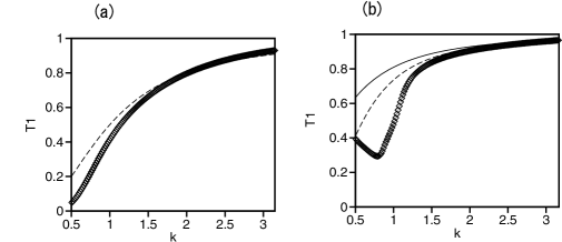
For the nonlinear splitter, a coarse approximation for the transmission coefficient is given by Eq. (33) with $\varepsilon_{0}$ replaced by $\varepsilon_{2}A^{2}$, cf. Eq. (16):

$$T_{1}=k^{2}/(k^{2}+\varepsilon_{2}^{2}A^{4})$$ (34)

Figure 2(b) shows that the discrepancy of this approximation at small $k$ is essentially larger than in the case of the linear splitter. The plots are not extended to $k<0.5$, as in that case the simulations do not show clear separation between the slowly moving broad transmitted and reflected pulses.

III.2 The operation of the “idle” interferometer in the linear regime

Proceeding to modeling the work of the interferometer, with the original splitting and subsequent recombination, it is natural to start with the linear model, based on Eq. (2) with $g=\varepsilon_{2}=0$, $\varepsilon_{0}>0$. Note that the target which should be detected by the interferometer is not introduced yet, therefore we name the setting “idle”. As above, a shifted Gaussian pulse (31) is used as the input.

The outcome of the linear operational cycle may be predicted as the product of the two scattering events, approximated by amplitudes (14). In the framework of the linear model, each secondary pulse acquires the same additional phase in the course of the half-oscillation in the HO trap between the two events, therefore this phase shift cancels in the analysis. Thus, the effective transmission and reflection amplitudes for routing the incident pulse to the right and left are, respectively, $2r\tau=2i|\tau||r|e^{2i\theta}$ and $\tau^{2}-r^{2}=(|\tau|^{2}-|r|^{2})e^{2i\theta}$. Accordingly, the overall transmission coefficient is

$$T_{2}=|2r\tau|^{2}=4T_{1}(1-T_{1}),$$ (35)

where $T_{1}$ is the transmission coefficient for the first collision given by Eq. (33), and relation $|r|^{2}+|\tau|^{2}=1$ is taken into regard.

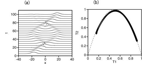
Equation (35) predicts $T_{2}=1$ in the case of $T_{1}=1/2$, i.e., complete recombination of the secondary pulses, after the second collision, into the Gaussian pulse moving in the original direction (to the right). The full simulation of the linear model, displayed in Fig. 3(a) for parameters corresponding to $T_{1}\approx 0.56$ indeed demonstrates virtually complete merger of the split pulses. In addition, Fig. 3(b) demonstrates that Eq. (35) very accurately approximates data collected from the direct simulations.

Figure 3: (a) The evolution of the Gaussian pulse with the center initially placed at $x=-18$, in the case of the linearized GPE (2) with $g=0$, $\Omega^{2}=0.004$ and $\varepsilon_{0}=1$, $\varepsilon_{2}=0$. In this case, Eqs. (32) and (33) yield $T_{1}\approx 0.56$. (b) The relation between the transmission coefficients corresponding to the primary splitting and subsequent  recombination, $T_{1}$ and $T_{2}$, in the same system. The chain of symbols and dashed line show, respectively, numerical results and analytical approximation (35).

III.3 The operation of the idle soliton-based interferometer with the linear splitter

Addressing the splitting and subsequent recombination of soliton (8) in the model based on Eq. (2) with $g=1$, we expect that a phase difference, $\Delta\theta=(T_{1}A^{2}-R_{1}A^{2})(\pi/2\Omega)$ is added to the pair of secondary (split) solitons at the moment of their collision ($t=\pi/\Omega$), due to the growth of their phases in time, as $(T_{1}A^{2}/2)t$ and $(R_{1}A^{2}/2)t$, after the splitting induced by the first collision (here, $R_{1}\equiv|r_{1}|^{2}=1-T_{1}$ is the respective reflection coefficient). Then, the eventual transmission coefficient may be evaluated as

$$T_{2}=T_{1}(1-T_{1})|1+e^{i\Delta\theta}|^{2}=2T_{1}(1-T_{1})[1+\cos\{(2T_{1}-1)A^{2}(\pi/2\Omega)\}],$$ (36)

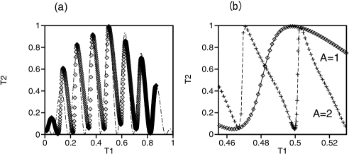
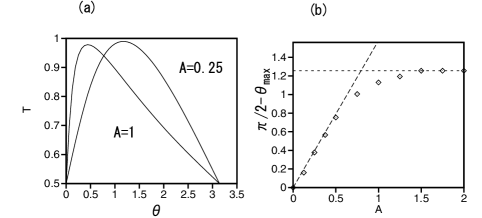
which oscillates sinusoidally as a function of $T_{1}$. Figure 4(a) shows the relation between $T_{1}$ and $T_{2}$, as obtained from numerical simulations. It is compared to the analytical approximation (36), which shows good agreement. Figure 4(b) zooms the relation around $T_{1}=0.5$. Note that smooth moderately asymmetric oscillations observed for $A=1$ are replaced by strongly asymmetric sawtooth-like oscillations for $A=2$, which corresponds to stronger background nonlinearity. Figure 3 clearly identifies a point of the virtually perfect recombination ($T_{2}=1$) very close to $T_{1}=0.5$, and a series of satellite points with gradually deteriorating recombination quality ($T_{2}<1$).

Figure 4: (a) The relation between the transmission coefficients corresponding to the original splitting and subsequent  recombination of the soliton, $T_{1}$ and $T_{2}$, in the model of the soliton-based interferometer (“idle”, i.e., without the target to be detected) in the model based on Eq. (2) with $\Omega^{2}=0.004$, $\varepsilon_{0}=1$, and $\varepsilon_{2}=0$. The soliton’s amplitude is $A=1,$ see Eq. (8).The chain of symbols and dashed line show, respectively, numerical results and the analytical prediction provided by Eq. (36). (b) A zoom of (b) around $T_{1}=0$, for $A=1$ and $A=2$.

To understand the asymmetric behavior observed in Fig. 4(b) in the case of the strong nonlinearity, we have performed numerical simulations of Eq. (2) for the collision of two solitons with a phase shift, $\theta$, taking the initial condition as

$$\phi=A\left\{\mathrm{sech}\left[A(x+x_{0})\right]+e^{i\theta}\mathrm{sech}\left[A(x-x_{0})\right]\right\}.$$ (37)

Figure 5(a) shows the corresponding recombination rate (defined as the integral transmission coefficient toward $x>0$, $T=\int_{0}^{\infty}|\phi(x)|^{2}dx/\int_{-\infty}^{+\infty}|\phi(x)|^{2}dx$), calculated at some moment of time after the end of the complete or incomplete collision-induced recombination. It is seen that, if $A$ is sufficiently small, a smooth quasi-sinusoidal dependence of $T$ on $\theta$ is observed, which changes to sawtooth-like oscillations as $A$ increases, i.e., the nonlinearity gets stronger. The quasi-sinusoidal behavior is due to the linear combination of the reflected and transmitted waves in the nearly-linear regime,

$$T\sim\left(1/2)\{|i|\tau|+|r|e^{i\theta}\right|^{2}\}=(1/2)+|r||\tau|\sin\theta,$$ (38)

see Eq. (14). Phase $\theta_{\max}$ corresponding to the largest recombination rate, which is $\theta=\pi/2$ in Eq. (38), deviates from $\pi/2$ as $A$ increases, due to the nonlinearity-induced phase shift. Figure 5(b) shows the deviation, $\pi/2-\theta_{\max}$, as a function of $A$.

Figure 5: (a) The relation between the recombination rate, $T$, and the phase shift, $\theta$, of the two colliding solitons, taken per Eq. (37) with amplitudes $A=0.25$ and $1$, as obtained from simulations of Eq. (2) with $g=1$, $\Omega^{2}=0.004$, $\varepsilon_{0}=1,$ $\varepsilon_{2}=0$. (b) $\pi/2-\theta_{\max}$ vs. $A$, where $\theta_{\max}$ is the phase shift in input (37) which produces the largest recombination rate. The dashed straight line in (b) is a linear fit for small $A$, $\pi/2-\theta_{\max}\approx 1.58A$.

The steep dependence of the recombination rate on $\theta$ is promising for the operation of the interferometer, with the target placed into one of its arms, as such a dependence may be used to secure high sensitivity of the operation, see below. It is relevant to mention that a similar transition from a smooth dependence to steep one with the increase of the nonlinearity strength was reported, for a soliton interferometer with a linear splitter, in Ref. Martin (see Figs. 1(d,e) in that work). Thus, Fig. 5(a) suggests that the accuracy of the interferometer using the linear splitter should improve if heavier solitons are used, with larger $A$. On the other hand, the increase of $A$ is limited by the fact that the solitons with the amplitude exceeding the critical value $A_{\mathrm{c}}^{(0)}$, given by Eq. (28) (or, strictly speaking, by its numerically generated counterpart), may not split at all. In particular, for $\varepsilon_{0}=1$ considered above, Eq. (28) suggests that only values $A<4$ may be usable.

III.4 The operation of the idle soliton-based interferometer with the nonlinear splitter

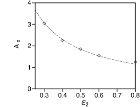
Prior to the simulations of the full soliton-based interferometer model using the nonlinear splitter, with $\varepsilon_{0}=0$ and $\varepsilon_{2}>0$ in Eq. (2), it makes sense to study, in some detail, the primary collision of soliton (8) with the nonlinear potential barrier. An essential prediction of the analysis reported in the previous section is that collision will lead to splitting of the incident soliton if its amplitude exceeds the critical value, which is given by Eq. (27) (on the contrary to the case of the linear barrier, which splits the soliton if its amplitude is smaller than the corresponding critical value, see Eq. (28)). Simulations corroborate the prediction, and produce the critical value, $A_{\mathrm{c}}$, which is displayed as a function of $\varepsilon_{2}$ in Fig. 6. The numerically found dependence may be fitted to

$$A_{\mathrm{c}}=0.92/\varepsilon_{2},$$ (39)

which yields larger values than the analytical estimate (27), but the dependence on $\varepsilon_{2}$ is essentially the same as predicted. The discrepancy in the overall factor ($0.92$ versus $0.5$) is explained by the fact that analytical consideration did not take into account deformation of the soliton’s shape in the course of the splitting.

Figure 6: The critical amplitude of the incident soliton, $A_{\mathrm{c}}$, above which it is split by the collision with the nonllinear potential barrier of strength $\varepsilon_{2}$, see Eq. (2). The dashed line shows the fit given by Eq. (39).

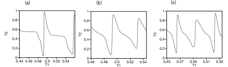
Proceeding to modeling the full scheme (but still for the interferometer in the idle mode), Fig. 7 shows relations between $T_{2}$ and $T_{1}$, similar to those displayed in Fig. 4 for the interferometer with the linear splitter, at different values of the amplitudes. The smallest one is chosen as $A=1.7$ because Eq. (39) shows that the incident soliton may be split by the nonlinear barrier with $\varepsilon_{2}=0.6$, considered here, only for $A>\allowbreak 1.\,\allowbreak 53$. Sharp sawtooth oscillations are observed in all the cases. The period of the oscillations increases with $A$, similar to what was seen for the model with the linear splitter. However, on the contrary to that model, in which the asymmetry and sharpness monotonically increase with $A$, here they are largest for the smallest amplitude considered, $A=1.7$. This finding is naturally explained by the fact that the variation must indeed be steepest closer to critical point. Because the steepest variation suggests the highest sensitivity, the use of the nonlinear splitter is potentially more promising than of its linear counterpart. Also promising is the fact that a relatively light soliton, which is easier to make in the experiment, will provide the higher accuracy. On the other hand, quantum fluctuations may come into the play for very light solitons quantum ; Helm .

Figure 7: Numerically generated relations between the transmission coefficients corresponding to the original splitting and subsequent  recombination of the soliton, $T_{1}$ and $T_{2}$ (cf. Fig. 3), in the model of the soliton-based interferometer (idle, i.e., without the target to be detected), in the model based on Eq. (2) with $\Omega^{2}=0.004$ and the nonlinear splitter: $\varepsilon_{0}=0$, $\varepsilon_{2}=0.6$. The amplitude of the incident soliton is $A=1.7$ in (a), $A=2$ in (b), and $A=2.3$ in (c).

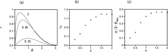
As suggested by the above analysis of the scheme with the linear potential barrier (see Fig. 5), the operation of the setup with the nonlinear splitter should be further characterized by the consideration of the on-splitter collision of two solitons with the same amplitude $A$ and phase shift $\theta$, corresponding to input (37). Figure 8 displays numerically generated dependences of the recombination rate, $T$, on $\theta$, for several values of the amplitude. It is seen that the largest value of $T$ increases with $A$, as well the deviation of the phase shift, $\theta_{\max}$, providing the largest value, from $\pi/2$. These dependences are markedly different from their counterparts in the model with the linear splitter, cf. Fig. 5.

Figure 8: (a) The relation between the recombination rate, $T$, and the phase shift, $\theta$, of the two colliding solitons, taken per Eq. (37) with amplitudes $A=0.25$, $0.85$, and $2$, as obtained from simulations of Eq. (2) with $g=1$, $\Omega^{2}=0.004$, $\varepsilon_{0}=0,$ $\varepsilon_{2}=0.6$. Value $A=0.85$ corresponds to Fig. 7(a). (b) The largest (peak) value, $T_{\mathrm{p}}$, of the recombination rate, which may be attained at given $A$, vs. $A$. (c) $\pi/2-\theta_{\max}$ vs. $A$, where $\theta_{\max}$ is the phase shift in input (37) which produces the largest recombination rate.

III.5 The operation of the loaded soliton-based interferometer

The most important step of the analysis is its application to the model of the interferometer in which one arm is “loaded” with the target that should be detected by the device. The above results, which demonstrate strong dependence of the recombination on phase changes suggest that the detection procedure may be quite sensitive.

The model of the loaded interferometer is derived from Eq. (2) (with $g=1$) by adding the target in the form of the $\delta$-functional linear potential placed at $x=x_{0}/2$, with strength $\varepsilon_{3}$:

$$i\frac{\partial\phi}{\partial t}=\left[-\frac{1}{2}\frac{\partial^{2}}{\partial x^{2}}-|\phi|^{2}+\frac{1}{2}\Omega^{2}x^{2}+\varepsilon_{0}\delta(x)+\varepsilon_{2}\delta(x)|\phi|^{2}+\varepsilon_{3}\delta\left(x-\frac{x_{0}}{2}\right)\right]\phi.$$ (40)

Note that $\varepsilon_{3}$ may be both positive and negative (repulsive or attractive), unlike $\varepsilon_{0}$ and $\varepsilon_{2}$ which should be positive to work as splitters (in principle, incident solitons hitting a local potential well may feature splitting too Brand ). Simulations of this model aimed to produce the recombination rate as a function of $\varepsilon_{3}$ for different values of the soliton’s amplitude, $A$. Here, we present results obtained for the case when the largest (peak) value of the recombination rate (as above, it is defined as the transmission coefficient, $T_{2}$, produced by the collision of the secondary solitons) is close to $T_{\mathrm{p}}=0.5$ at $\varepsilon_{3}=0$, which actually implies the choice of parameters at which the recombination does not occur in the idle interferometer.

First, Fig. 9(a) shows the dependence of the recombination rate on the target’s strength, $\varepsilon_{3}$, in the interferometer using the linear splitter with $\varepsilon_{0}=1,\varepsilon_{2}=0$. It is observed that $T_{2}$ varies very smoothly at $A=0.5$. To quantify the sensitivity, we have defined it as the value of $dT_{2}/d\varepsilon_{3}$ at $\varepsilon_{3}=0$. Figure 9(b) shows its dependence on the initial amplitude of the probe soliton.

Figure 9: (a) The dependence of the recombination rate, $T_{2}$, on the target’s strength, $\varepsilon_{3},$ for two values of the initial amplitude of the probe soliton, $A=$ $0.5$ and $1.5$, produced by simulations of Eq. (40) with the linear splitter, $\varepsilon_{0}=1,\varepsilon_{2}=0$. (b) The dependence of the sensitivity, $dT_{2}/d\varepsilon_{3}$ at $\varepsilon_{3}=0$, for the same system.

Figure 10: The same as in Fig. 9, but for the system with the nonlinear splitter ($\varepsilon_{0}=0,\varepsilon_{2}=0.6$), at three values of the initial amplitude of the probe soliton: $A=2.0,2.125$, and $2.3$.

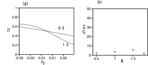
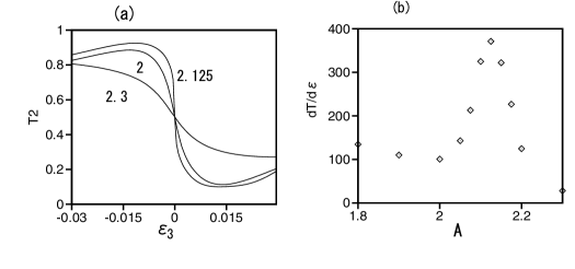
Next, Fig. 10(a) shows the most essential results produced by the analysis, i.e., $T_{2}$ as a function of $\varepsilon_{3}$, and the sensitivity, $dT_{2}/d\varepsilon_{3}$ at $\varepsilon_{3}=0$, as a function of the initial soliton’s amplitude, $A$ in the system using the nonlinear splitter, with $\varepsilon_{0}=0,\varepsilon_{2}=0.6$. In this case, $T_{2}$ varies much faster near $\varepsilon_{3}=0$, and the sensitivity is much higher in comparison with the setup using the linear splitter, cf. Fig. 9. In particular, the sensitivity takes a very large value $370$ near $A=2.125$, as shown in Fig. 10(b). A relative width of the high-sensitivity region is $\Delta A/A\simeq 0.03$, implying that the optimal use of the present setup requires rather accurate selection of parameters of the probe soliton, which may be a challenge to the implementation of the present scheme. In principle, if a stable source of solitons is available, such as a matter-wave soliton laser laser , the scheme may be adjusted to the optimal operation regime empirically, by tuning parameters of the optical beam which controls the action of the nonlinear splitter. However, a discussion of further details of the experimental implementation does not seem relevant in this theoretical paper.

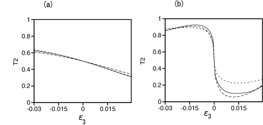
While the highest sensitivity is attained at $\varepsilon_{2}=0.6$, similar results were obtained for other values of strength $\varepsilon_{2}$, with lower values of the largest sensitivity, which is $26$ at $\varepsilon_{2}=0.7$, and $102$ at $\varepsilon_{2}=0.5$. It was also checked that the results reported in this subsection are robust in the sense that they do not vary conspicuously with the change of width $\Delta x$ used for the approximation of the $\delta$-function. The robustness is illustrated by Fig. 11, which demonstrates that findings collected in Figs. 9(a) and 10(a) vary weakly with $\Delta x$. Thus, the use of the nonlinear splitter offers the possibility to build very efficient soliton-based interferometers, in comparison with the previously developed setups, that use the linear splitter.

Figure 11: (a) and (b): The same as in Figs. 9(a) for $A=1.5$ and 10(a) for $A=2.125$, respectively, but with widths $\Delta x=0.2$ (long-dash lines), $0.4$ (solid lines), and $0.6$ (short-dash lines) of the finite barrier approximating the $\delta$-function.

IV Conclusion

We have introduced the model of the soliton-based interferometer which utilizes, unlike the previously studied schemes, the nonlinear splitter, in the form of the localized region with the strongly repulsive intrinsic nonlinearity, embedded into the uniform self-attractive medium. It was demonstrated that this setting may be realized with the help of the Feshbach resonance, controlled by a laser beam focused on a narrow region, where it creates the repulsive nonlinearity. The systematic analysis of the scattering of plane waves and solitons on the localized nonlinear potential, and of the operation of the full interferometric setup, has been carried out by means of combined analytical and numerical methods. For the sake of comparison with the new setup, additional analysis was also developed for the traditional one, based on the linear splitter. Essential results include the exact solution for the scattering of the plane wave in the linear medium on the nonlinear $\delta$-functional nonlinear potential and perturbative analysis of the splitting of the incident solitons by the same potential. The most significant finding is that the use of the nonlinear splitter predicts operational regimes for the interferometer with the sensitivity to the target much higher than provided, in the same range of parameters, by the usual linear splitter.

The work may be extended by considering the generalized form of the GPE which takes into account deviations from the one-dimensionality, making use of approaches developed in Refs. 1D3D and Cuevas . Another interesting possibility is the use of probe solitons with embedded vorticity, cf. Ref. Luca-vortex .

References

- (1) Strecker K E, Partridge G B, Truscott A G, and Hulet R G 2002 Nature 417 150 Khaykovich L, Schreck F, Ferrari G, Bourdel T, Cubizolles J, Carr L D, Castin Y, and Salomon C 2002 Science 296 1290 Strecker K E, Partridge G B, Truscott A G, and Hulet R G 2003 New J. Phys. 5 73.1 Medley P, Minar M A, Cizek N C, Berryrieser D, and Kasevich M A 2014 Phys. Rev. Lett. 112 060401
- (2) Cornish S L, Thompson S T, and Wieman C E 2006 Phys. Rev. Lett. 96 170401
- (3) Marchant A L, Billam T P, Wiles T P, Yu M M H, Gardiner S A, and Cornish S L 2013 Nature Comm. 4 1865
- (4) Nguyen J H V, Dyke P, Luo D, Malomed B A, and Hulet R G 2014 Nature Phys. 10 918
- (5) Veretenov N, Rozhdestvenskya Yu, Rosanov N, Smirnov V, and Fedorov S, Eur. Phys. J. D 2007 42 455 Abdullaev F Kh and Brazhnyi V A 2012 J Phys B: At Mol Opt Phys 45 085301 Gertjerenken B and Weiss C 2012 J Phys B: At Mol Opt Phys 45 165301 Kageyama Y and Sakaguchi H 2012 J. Phys. Soc. Jpn. 81 033001 Gertjerenken B 2013 Phys. Rev. A 88 053623 Polo J and Ahufinger V 2013 Phys. Rev. A 88 053628 Helm J L, Cornish S L, and Gardiner S A 2015 Phys Rev Lett 114 134101
- (6) Martin A D and Ruostekoski J 2012 New J. Phys. 14 043040
- (7) Helm J L, Billam T P, and Gardiner S A 2012 Phys. Rev. A 85 053621
- (8) Helm J L,Rooney S J, Weiss C, and Gardiner S A 2014 Phys. Rev. A 89 033610
- (9) McDonald G D, Kuhn C C N, Hardman K S, Bennetts S, Everitt P J, Altin P A, Debs J E, Close J D, and Robins N P 2014 Phys Rev Lett 113 013002
- (10) Cuevas J Kevrekidis P G Malomed B A Dyke P and Hulet R G 2013 New J. Phys. 15 063006
- (11) Carr L D, Miller R R, Bolton D R, and Strong S A 2012 Phys. Rev. A 86 023621
- (12) Banchi L, Compagno E, and Bose S 2015 Phys. Rev. A 91 052323
- (13) Gertjerenken B, Billam T P, Khaykovich L, and Weiss C 2012 Phys. Rev. A 86 033608 Banchi L, Compagno E, and Bose S 2015 Phys. Rev. A 91 052232.
- (14) Li S C and Dou F-D 2015 EPL 111 30005
- (15) Billam T P, Cornish S L, and Gardiner S A 2011 Phys. Rev. A 83 041602(R)
- (16) Orzel C, Tuchman A K, Fenselau M L, Yasuda M, and Kasevich M A 2001 Science 291 2386
- (17) Pitaevskii L P and Stringari A 2003 Bose-Einstein Condensation (Clarendon Press, Oxford).
- (18) Kartashov Y V, Malomed B A, and Torner L, Rev. Mod. Phys. 2011 83 247
- (19) Maor O, Dror N, and Malomed B A 2013 Opt. Lett. 38 5454
- (20) Hukriede J, Runde D, and Kip D 2003 J. Phys. D 36, R1
- (21) Malomed B A 2015 Nature Phot. 9 287
- (22) Salasnich L, Parola A, and Reatto L 2002 Phys. Rev. A 65 043614 Muryshev A E, Shlyapnikov G V, Ertmer W, Sengstock K, and Lewenstein M 2002 Phys. Rev. Lett. 89 110401 Muñoz Mateo A and Delgado V 2008 Phys. Rev. A 77 013617
- (23) Salasnich L, Malomed B A, and Toigo F 2007 Phys. Rev. A 76 063614.
- (24) Fedichev P O, Kagan Y, Shlyapnikov G V, and Walraven J T M 1996 Phys. Rev. Lett. 77 2913 Theis M, Thalhammer G, Winkler K, Hellwig M, Ruff G, Grimm R, and Denschlag J H 2004 Phys. Rev. Lett. 93 123001 Bauer D M, Lettner M, Vo C, Rempe G, and Dürr S 2009 Nature Phys. 5 339 Yamazaki R, Taie S, Sugawa S, and Takahashi Y 2010 Phys. Rev. Lett. 105 050405 Yan M, DeSalvo B J, Ramachandhran B, Pu H, and Killian T C 2013 Phys. Rev. Lett. 110 123201 Clark L W, Ha L-C, Xu C-Y, and Chin C 2015 Phys. Rev. Lett. 115 155301
- (25) Mickelson P G, Matrtinez de Escobar Y N, Yan M, DeSalvo B I, and Killian T C 2010 Phys. Rev. A 81 051601(R)
- (26) Nicholson T L, Blatt S, B. J. Bloom B J, Williams J R, Thomsen J R, Ye J and Julienne P S 2015 Phys. Rev. A 92 022709
- (27) Marchant A L, Billam T P, Yu M M H, Rakonjac A, Helm J L, Polo J, Weiss C, Gardiner S A, and Cornish S L 2015 arXiv:1507.04639
- (28) Griffiths D J, Introduction to Quantum Mechanics (2nd ed.) (Prentice Hall, 2005)
- (29) Malomed B A and Azbel M Ya 1993 Phys. Rev. B 1993 47 10402
- (30) Kivshar Yu S and Malomed B A 1989 Rev. Mod. Phys. 763
- (31) Ernst T and Brand J 2010 Phys. Rev. A 81 033614
- (32) Carr L D and Brand J 2004 Phys. Rev. A 70 033607 Carpentier A V, Michinel H, and Rodas-Verde M I 2006 Phys. Rev. A 74 013619 Chen P Y P and Malomed B A 2006 J. Phys. B: At. Mol. Opt. Phys. 39 2803