Stabilization of Systems with Asynchronous Sensors and Controllers

Abstract

We study the stabilization of networked control systems with asynchronous sensors and controllers. Offsets between the sensor and controller clocks are unknown and modeled as parametric uncertainty. First we consider multi-input linear systems and provide a sufficient condition for the existence of linear time-invariant controllers that are capable of stabilizing the closed-loop system for every clock offset in a given range of admissible values. For first-order systems, we next obtain the maximum length of the offset range for which the system can be stabilized by a single controller. Finally, this bound is compared with the offset bounds that would be allowed if we restricted our attention to static output feedback controllers.

I Introduction

In networked and embedded control systems, the outputs of plants are often sampled in a nonperiodic fashion and sent to controllers with time-varying delays. To address robust control with such imperfections, various techniques have been developed, for example, the input-delay approach [11, 22], the gridding approach [12, 25, 7], and the impulsive systems approach based on Lyapunov functionals [23], on looped functionals [4], and on clock-dependent Lyapunov functions [3]; see also the surveys [17, 18]. In contrast to the references mentioned above, here we assume that time-stamps are used to provide the controller with information about the sampling times and the communication delays incurred by each measurement. In this approach, sensors send measurements to controllers together with time-stamps, and the controllers exploit this information to mitigate the effect of variable delays and sampling periods [15, 24, 13]. However, when the local clocks at the sensors and at the controllers are not synchronized, the time-stamps and the true sampling instants do not match. Protocols to establish synchronization have been actively studied as surveyed in [28], and synchronization by the global positioning system (GPS) or radio clocks has been utilized in some systems. Nevertheless, synchronizing clocks over networks has fundamental limits [10], and a recent study [19] has shown that synchronization based on GPS signals is vulnerable against attacks.

In this paper, we study the stabilization problem of systems with asynchronous sensing and control. We assume that the controller can use the time-stamps but does not know the offset between the sensor and controller clocks, but we do assume that this offset is essentially constant over the time scales of interest. Our objective is to find linear time-invariant (LTI) controllers that achieve closed-loop stability for every clock offset in a given range.

We formulate the stabilization of systems with clock offsets as the problem of stabilizing systems with parametric uncertainty, which can be regarded as the simultaneous stabilization of a family of plants, as studied in [32, Sec. 5.4] and [33]. However, we had to overcome a few technical difficulties that distinguish the problem considered here from previously published results:

Infinitely many plants: We consider a family of plant models that is indexed by a continuous-valued parameter. Such a family includes infinitely many plants, but the approaches for simultaneous stabilization e.g., in [30] exploit the property that the number of plant models is finite.

Nonlinearity of the uncertain parameter: In this work, the uncertain parameter appears in a non-linear form. Therefore, it is not suitable to use the techniques based on linear matrix inequalities (LMIs) in [6] for the robust stabilization of systems with polytopic uncertainties. Although the robust stability analysis based on continuous paths of systems with respect to the $\nu$-gap metric was developed in [5], controller designs based on this approach have not been fully investigated.

Common unstable poles and zeros: Earlier studies on simultaneous stabilization consider a restricted class of plants. For example, the sufficient condition in [2] is obtained for a family of plants with no common unstable zeros or poles. The set of plants in [21] has common unstable zeros (or poles) but all the plants are stable (or minimum-phase). These assumptions are not satisfied for the systems in the present paper.

We make the following technical contributions for multi-input systems and first-order systems: First we consider multi-input systems and obtain a sufficient condition for stabilization with asynchronous sensing and control. We construct a stabilizing controller from the solution of an appropriately defined $\mathcal{H}^{\infty}$ control problem. The above mentioned difficulties found in the simultaneous stabilization problem we consider is circumvented by exploiting geometric properties on $\mathcal{H}^{\infty}$. For first-order systems, we obtain an explicit formula for the exact bound on the clock offset that can be allowed for stability. This result is based on the stabilization of interval systems [14, 27], to which our problem can be reduced for first-order plants. We start by formulating the problem in the context of state feedback without disturbances and noise, but we show in Section 3.2 that the above results also apply for output feedback with disturbances and noise.

The authors in the previous study [26] have considered systems with time-varying clock offsets and have proposed a stabilization method with causal controllers, based on the analysis of data rate limitations in quantized control. The stability analysis and the $\mathcal{L}^{2}$-gain analysis of systems with variable clock offsets have been investigated in [34] and [36], respectively. The major difference with respect to those studies is that here we consider only constant offsets but design stabilizing LTI controllers. This paper is based on the conference paper [35], but here we extend the preliminary results for single-input systems to the multi-input case.

The remainder of the paper is organized as follows. Section 2 introduces the closed-loop system we consider and presents the problem formulation. Section 3 is devoted to the discretization of the closed-loop system. In Section 4, we obtain a sufficient condition for the stabilizability of general-order systems. In Section 5, we derive the exact bound on the permissible clock offset for first-order systems. In Section 6, we discuss stabilizability with static controllers and the comparison of the offset bounds obtained for LTI controllers and static controllers.

Notation and definitions:  We denote by $\mathbb{Z}_{+}$ the set of non-negative integers. The symbols $\mathbb{D}$, $\bar{\mathbb{D}}$, and $\mathbb{T}$ denote the open unit disc $\{z\in\mathbb{C}:~{}|z|<1\}$, the closed unit disc $\{z\in\mathbb{C}:~{}|z|\leq 1\}$, and the unit circle $\{z\in\mathbb{C}:~{}|z|=1\}$, respectively. We denote by $\mathbb{D}^{c}$ the complement of the open unit disc $\{z\in\mathbb{C}:~{}|z|\geq 1\}$.

A square matrix $F$ is said to be Schur stable if all its eigenvalues lie in the unit disc $\mathbb{D}$. We say that a discrete-time LTI system $\xi_{k+1}=F\xi_{k}+Gu_{k},~{}y_{k}=H\xi_{k}$ is stabilizable (detectable) if there exists a matrix $K$ ($L$) such that $F-GK$ ($F-LH$) is Schur stable. We also use the terminology $(F,G)$ is stabilizable (respectively, $(F,H)$ is detectable) to denote this same concept.

We denote by $\mathcal{RH}^{\infty}$ the space of all bounded holomorphic real-rational functions in $\mathbb{D}$. The field of fractions of $\mathcal{RH}^{\infty}$ is denoted by $\mathcal{RF}^{\infty}$. For a commutative ring $R$, $\mathbf{M}(R)$ denotes the set of matrices with entries in $R$, of any order. For $M\in\mathbf{M}(\mathbb{C})$, $\|M\|$ denotes the induced 2-norm. For $G\in\mathbf{M}(\mathcal{RH}^{\infty})$, the $\mathcal{RH}^{\infty}$-norm is defined as $\|G\|_{\infty}=\sup_{z\in\mathbb{D}}\|G(z)\|$. For $G=\begin{bmatrix}G_{11}&\quad G_{12}\\ G_{21}&\quad G_{22}\end{bmatrix}\in\mathbf{M}(\mathcal{RF}^{\infty})$ and $Q\in\mathbf{M}(\mathcal{RF}^{\infty})$, we define a lower linear fractional transformation of $G$ and $Q$ as $\mathcal{F}_{\ell}(G,Q):=G_{11}+G_{12}Q(I-G_{22}Q)^{-1}G_{21}$.

A pair $(N,D)$ in $\mathbf{M}(\mathcal{RH}^{\infty})$ is said to be right coprime if the Bezout identity $XN+YD=I$ holds for some $X$, $Y\in\mathbf{M}(\mathcal{RH}^{\infty})$. $P\in\mathbf{M}(\mathcal{RF}^{\infty})$ admits a right coprime factorization if there exist $D$, $N\in\mathbf{M}(\mathcal{RH}^{\infty})$ such that $P=ND^{-1}$ and the pair $(N,D)$ is right coprime. Similarly, a pair $(\tilde{D},\tilde{N})$ in $\mathbf{M}(\mathcal{RH}^{\infty})$ is left coprime if the Bezout identity $\tilde{N}\tilde{X}+\tilde{D}\tilde{Y}=I$ holds for some $\tilde{X}$, $\tilde{Y}\in\mathbf{M}(\mathcal{RH}^{\infty})$. $P\in\mathbf{M}(\mathcal{RF}^{\infty})$ admits a left coprime factorization if there exist $\tilde{D}$, $\tilde{N}\in\mathbf{M}(\mathcal{RH}^{\infty})$ such that $P=\tilde{D}^{-1}\tilde{N}$ and the pair $(\tilde{D},\tilde{N})$ is left coprime. If $P$ is a scalar-valued function, then we use the expressions coprime and coprime factorization.

II Problem Statement

Consider the following LTI plant:

$$\Sigma_{P}:~{}\dot{x}(t)=Ax(t)+Bu(t),$$ (1)

where $x(t)\in\mathbb{R}^{n}$ and $u(t)\in\mathbb{R}^{m}$ are the state and the input of the plant, respectively. As shown in Fig. 1, this plant is connected through a sampler and a zero-order hold (ZOH) to a time-stamp aware estimator and a controller, which will be described soon.

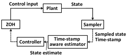
Figure 1: Closed-loop system with a time-stamp aware estimator.

Let $s_{1},s_{2},\dots$ be sampling instants from the perspective of the controller clock. A sensor measures the state $x(s_{k})$ and sends it to a controller together with a time-stamp. However, since the sensor and the controller may not be synchronized, the time-stamp determined by the sensor typically includes an unknown offset with respect to the controller clock. In this paper, we assume that the clock offset is constant. Although clock properties are affected by environment such as temperature and humidity, the change of such properties is slow for the time scales of interest. Furthermore, the difference of clock frequencies can be ignored. This is justified by noting that time synchronization techniques, like the one proposed in [16], can achieve asymptotic convergence of the clock frequencies (in the mean-square sense), even in the presence of random network delays. We thus assume that the time-stamp $\hat{s}_{k}$ reported by the sensor is given by

$$\hat{s}_{k}=s_{k}+\Delta\qquad(k\in\mathbb{N})$$ (2)

for some unknown constant $\Delta\in\mathbb{R}$.

Let $h>0$ be the update period of the ZOH. The control signal $u(t)$ is assumed to be piecewise constant and updated periodically at times $t_{k}=kh$ ($k\in\mathbb{N}$) with values $u_{k}$ computed by the controller: $u(t)=u_{k}$ for $t\in[t_{k},t_{k+1})$. We place a basic assumption for stabilization of sampled-data systems.

Assumption II.1

(Stabilizability and non-pathological control update) The plant $(A,B)$ is stabilizable and the update period $h$ is non-pathological, that is, $(\lambda_{p}-\lambda_{q})h\not=2\pi j\ell$ ($\ell=\pm 1,\pm 2,\dots$) for each pair $(\lambda_{p},\lambda_{q})$ of eigenvalues of $A$.

While the ZOH updates the control signal $u(t)$ periodically, the true sampling times $s_{k}$ and the reported sampling times $\hat{s}_{k}$ may not be periodic. However, we do assume that both $s_{k}$ and $\hat{s}_{k}$ do not fall behind $t_{k}$ by more than the ZOH update period $h$. This assumption is formally stated as follows.

Assumption II.2

(Bounded clock offset) For every $k\in\mathbb{Z}_{+}$, $s_{k},\hat{s}_{k}\in[t_{k},t_{k+1})$.

This assumption implies that the clock offset $\Delta$ is smaller than the control update period $h$, which holds in most mechatronics systems. In fact, control update periods for mechatronics systems generally take values from 100 $\mu$s to 10 ms, while recent clock synchronization algorithms such as the IEEE 1588 Precision Time Protocol (PTP) [1] make clock offsets smaller than a few tens of microseconds.

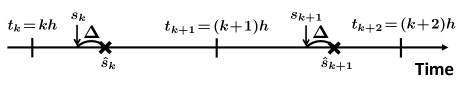
Figure 2: Sampling instants $s_{k}$, reported time-stamps $\hat{s}_{k}$, and updating instants $t_{k}$ of the zero-order hold.

Fig. 2 shows the timing diagram of the sampling instants $s_{k}$, the reported time-stamps $\hat{s}_{k}$, and updating instants $t_{k}$ of the control inputs.

The controller side is comprised of a time-stamp aware estimator and a controller as in the model-based or emulation-based control of networked control systems [13]. The time-stamp aware estimator generates the state estimate $\hat{x}(t_{k+1})\in\mathbb{R}^{n}$ from the data $(x(s_{k}),\hat{s}_{k})$ according to the following dynamics:

$$\Sigma_{E}:~{}\begin{cases}\dot{\hat{x}}(t)=A\hat{x}(t)+Bu(t)&\qquad(t_{k}<t\leq t_{k+1})\\ \hat{x}(\hat{s}_{k})=x(s_{k}),&\qquad(k\in\mathbb{Z}_{+}).\end{cases}$$ (3)

Note that if the time-stamp is correct, i.e., $s_{k}=\hat{s}_{k}$, then this estimator consistently produces $\hat{x}(t)=x(t)$ for all $t$, perfectly compensating transmission delays. Time-stamp aware estimators have been used to compensate for network-induced imperfections, e.g., in [15, 24, 13].

The controller is a discrete-time LTI system and generates the control input $u_{k}$ based on the state estimate $\hat{x}_{k}:=\hat{x}(t_{k})$:

$$\Sigma_{C}:~{}\begin{cases}\zeta_{k+1}=A_{c}\zeta_{k}+B_{c}\hat{x}_{k}\\ u_{k}=C_{c}\zeta_{k}+D_{c}\hat{x}_{k},\end{cases}$$ (4)

where $\zeta_{k}\in\mathbb{R}^{n_{c}}$ is the state of the controller.

The objective of the present paper is to find a discrete-time LTI controller $\Sigma_{C}$ as in (4) that achieves closed-loop stability for every clock offset in a given range of admissible values. Specifically, we want to solve the following problem:

Problem II.3

Given an offset interval $[\underline{\Delta},\overline{\Delta}]$, determine if there exists a controller $\Sigma_{C}$ as in (4) such that $x(t)$, $\hat{x}(t)\to 0$ as $t\to\infty$ and $\zeta_{k}\to 0$ as $k\to\infty$ for every $\Delta\in[\underline{\Delta},\overline{\Delta}]$ and for every initial states $x(0)$ and $\zeta_{0}$. Furthermore, if one exists, find such a controller $\Sigma_{C}$.

III Discretization of the Closed-loop System

To solve Problem II.3, we discretize the system comprised of the plant $\Sigma_{P}$, the estimator $\Sigma_{E}$, the ZOH, and the sampler. In this section, we obtain a realization for the discretized system and describe its basic properties related to stability, stabilizability, and detectability. Moreover, we extend the discretized system to scenarios with disturbances/noise and output feedback.

III-A Discretized system and its basic properties

The following lemma provides a realization for the discretized system:

Lemma III.1

Define

$$\xi_{k}:=\begin{bmatrix}x(t_{k})-\hat{x}(t_{k})\\ \hat{x}(t_{k})\end{bmatrix}.$$

The dynamics of the discretized system $\Sigma_{d}$ comprised of the plant $\Sigma_{P}$, the estimator $\Sigma_{E}$, the ZOH, and the sampler can be described by the following equations:

$$\Sigma_{d}:~{}\xi_{k+1}=F_{\Delta}\xi_{k}+G_{\Delta}u_{k},\qquad\eta_{k}=H_{\Delta}\xi_{k},$$ (5)

where $\Lambda:=e^{Ah}$, $\Theta:=e^{-A\Delta}-I$, and

$$F_{\Delta} :=\begin{bmatrix}-\Lambda\Theta&\quad-\Lambda\Theta\\ \Lambda(I+\Theta)&\quad\Lambda(I+\Theta)\end{bmatrix},\quad H_{\Delta}:=\begin{bmatrix}0&\quad I\end{bmatrix}$$

$$G_{\Delta} :=\begin{bmatrix}\Lambda\left(\int^{h}_{0}e^{-A\tau}d\tau-(I+\Theta)\int^{h-\Delta}_{0}e^{-A\tau}d\tau\right)B\\ \Lambda(I+\Theta)\int^{h-\Delta}_{0}e^{-A\tau}d\tau B\end{bmatrix}.$$ (6)

Proof: Using $\Lambda=e^{Ah}$, we have from the state equation (1) that

$$x(t_{k+1}) =\Lambda x(t_{k})+\Lambda\int^{h}_{0}e^{-A\tau}d\tau\cdot Bu_{k}.$$ (7)

We compute $\hat{x}(t_{k+1})$ in terms of $x(t_{k})$ and $u_{k}$. It follows from the dynamics of the estimator $\Sigma_{E}$ in (3) that

$$\hat{x}(t_{k+1})=e^{A(t_{k+1}-\hat{s}_{k})}\hat{x}(\hat{s}_{k})+\int^{t_{k+1}}_{\hat{s}_{k}}e^{A(t_{k+1}-\tau)}Bd\tau\cdot u_{k}$$ (8)

and

$$\hat{x}(\hat{s}_{k})=x(s_{k})=e^{A(s_{k}-t_{k})}x(t_{k})+\int^{s_{k}}_{t_{k}}e^{A(s_{k}-\tau)}Bd\tau\cdot u_{k}.$$ (9)

Since $t_{k+1}-t_{k}=h$ and $\hat{s}_{k}=s_{k}+\Delta$, it follows that

$$e^{A(t_{k+1}-\hat{s}_{k})}\cdot e^{A(s_{k}-t_{k})}=e^{A(h-\Delta)},$$ (10)

and also that

$$e^{A(t_{k+1}-\hat{s}_{k})}\int^{s_{k}}_{t_{k}}e^{A(s_{k}-\tau)}d\tau=\int^{\hat{s}_{k}}_{t_{k}+\Delta}e^{A(t_{k+1}-\tau)}d\tau.$$ (11)

Using $\Lambda=e^{Ah}$ and $\Theta=e^{-A\Delta}-I$, we conclude from (8)–(11) that

$$\hat{x}(t_{k+1}) =\Lambda(I+\Theta)x(t_{k})+\Lambda(I+\Theta)\int^{h-\Delta}_{0}e^{-A\tau}Bd\tau\cdot u_{k}.$$ (12)

From (7) and (12), we obtain the $F_{\Delta}$ and $G_{\Delta}$ in (6). Moreover, we have $H_{\Delta}=[0~{}~{}I]$ by the definition of the extended state $\xi_{k}$. $\Box$  ∎

Next we show that if the extended state $\xi_{k}$ and the controller state $\zeta_{k}$ converge to the origin, then the intersample values of $x$ and $\hat{x}$ also converge to the origin.

Proposition III.2

For the discreteized system $\Sigma_{d}$ in Lemma III.1, we have that $\xi_{k},\zeta_{k}\to 0$ as $k\to\infty$ if and only if $x(t),\hat{x}(t)\to 0$ as $t\to\infty$ and $\zeta_{k}\to 0$ as $k\to\infty$.

Proof: The statement that $x(t),\hat{x}(t)\to 0$ as $t\to\infty$ and $\zeta_{k}\to 0$ as $k\to\infty$ imply $\xi_{k},\zeta_{k}\to 0$ as $k\to\infty$, follows directly from the definition of $\xi_{k}$.

To prove the converse statement, assume that $\xi_{k},\zeta_{k}\to 0$ as $k\to\infty$. Then $\hat{x}(t_{k})=H_{\Delta}\xi_{k}\to 0$ and $x(t_{k})$, $u_{k}\to 0$ as $k\to\infty$. Since

$$\|x(t_{k}+\tau)\|\leq e^{\|A\|h}\|x(t_{k})\|+\int^{h}_{0}e^{\|A\|h}\|B\|dt\cdot\|u_{k}\|$$

for all $k\in\mathbb{Z}_{+}$ and all $\tau\in[0,h)$, we derive $x(t)\to 0$ ($t\to\infty$). Similarly, we see from the dynamics of the estimator $\Sigma_{E}$ that $\hat{x}(t)\to 0$ as $t\to\infty$. This completes the proof. $\Box$  ∎

This proposition allows us to conclude Problem II.3 can be solved by finding LTI controllers $\Sigma_{C}$ achieving $\xi_{k}$, $\zeta_{k}\to 0$ ($k\to\infty$) for every $\Delta\in[\underline{\Delta},\overline{\Delta}]$ and for every initial states $\xi_{0}$ and $\zeta_{0}$.

The following result allows us to conclude that the discretized system $\Sigma_{d}$ is detectable and stabilizable for all $\Delta$ and almost all $h$ if the plant $(A,B)$ is stabilizable.

Proposition III.3

The discretized system $\Sigma_{d}$ in (5) is detectable for all $\Delta$ and $h$. Moreover, $\Sigma_{d}$ is stabilizable for all $\Delta$ if Assumption II.1 holds.

Proof: Let us first obtain another realization $(\bar{F}_{\Delta},\bar{G}_{\Delta},\bar{H}_{\Delta})$ of the discretized system $\Sigma_{d}$ in (5). We can transform $F_{\Delta}$ into

$$\bar{F}_{\Delta} :=T^{-1}F_{\Delta}T=\begin{bmatrix}\Lambda&\quad 0\\ 0&\quad 0\end{bmatrix},\text{~{}~{}where~{}~{}}T:=\begin{bmatrix}-\Theta&\quad-I\\ I+\Theta&\quad I\end{bmatrix}.$$

Furthermore, if we define

$$J_{1}:=\int^{h}_{0}e^{-A\tau}d\tau,\qquad J_{2}:=\int^{h-\Delta}_{0}e^{-A\tau}d\tau,$$

then we obtain

$$\bar{G}_{\Delta}:=T^{-1}G_{\Delta}=\begin{bmatrix}\Lambda J_{1}B\\ -\Lambda(J_{1}-(I+\Theta)J_{2})B-\Theta\Lambda J_{1}B\end{bmatrix}$$

and $\bar{H}_{\Delta}:=H_{\Delta}T=[I+\Theta\quad I].$ We have thus another realization $(\bar{F}_{\Delta},\bar{G}_{\Delta},\bar{H}_{\Delta})$ for $\Sigma_{d}$.

Next we check detectability and stabilizability by using the realization $(\bar{F}_{\Delta},\bar{G}_{\Delta},\bar{H}_{\Delta})$. Define

$$L_{\Delta}:=\begin{bmatrix}\Lambda(I+\Theta)^{-1}\\ 0\end{bmatrix}.$$ (13)

Then we have that

$$\bar{F}_{\Delta}-L_{\Delta}\bar{H}_{\Delta}=\begin{bmatrix}0&-\Lambda(I+\Theta)^{-1}\\ 0&0\end{bmatrix},$$ (14)

and clearly $\bar{F}_{\Delta}-L_{\Delta}\bar{H}_{\Delta}$ is Schur stable. Therefore, the discreteized system $\Sigma_{d}$ is detectable for all $h$ and $\Delta$.

To show stabilizability, we use the well-known rank conditions (see, e.g., [40, Sec. 3.2]). We have that $[zI-\bar{F}_{\Delta}~{}~{}\bar{G}_{\Delta}]$ is full row rank for all $z\in\mathbb{D}^{c}$ if and only if

$$\begin{bmatrix}zI-\Lambda&\quad\Lambda J_{1}B\end{bmatrix}=\begin{bmatrix}zI-e^{Ah}&\quad\int^{h}_{0}e^{A\tau}Bd\tau\end{bmatrix}$$

is full row rank for all $z\in\mathbb{D}^{c}$. Hence, the discretized system $\Sigma_{d}$ is stabilizable for all $\Delta$ if Assumption II.1 holds.  ∎

III-B Extension to the output feedback case with disturbances and noise

Instead of $\Sigma_{P}$ in (1), consider a plant $\Sigma_{P}^{\prime}$ with disturbances, noise, and output feedback:

$$\Sigma_{P}^{\prime}:~{}\begin{cases}\dot{x}(t)=Ax(t)+Bu(t)+d(t)\\ y(t)=Cx(t)+n(t),\end{cases}$$

where $d(t)\in\mathbb{R}^{n}$ and $n(t)$, $y(t)\in\mathbb{R}^{p}$ are the disturbance, measurement noise, and output of the plant, respectively. As in [13, Chap. 3], [38], and the references therein, we assume that a smart sensor is co-located with the plant and that the sensor has the following observer to generate the state estimate, which is sampled and sent to the controller side:

$$\Sigma_{O}:~{}\dot{\bar{x}}(t)=A{\bar{x}}(t)+Bu(t)+L(y(t)-C\bar{x}(t)),$$

where $\bar{x}(t)\in\mathbb{R}^{n}$ is the state estimate and $L$ is an observer gain such that $A-LC$ is Hurwitz. The sampler sends the state estimate $\bar{x}$, and the resulting dynamics of the time-stamp aware estimator $\Sigma_{E}^{\prime}$ is provided by

$$\Sigma_{E}^{\prime}:~{}\begin{cases}\dot{\hat{x}}(t)=A\hat{x}(t)+Bu(t)&\qquad(t_{k}\leq t<t_{k+1})\\ \hat{x}(\hat{s}_{k})=\bar{x}(s_{k})+w_{k},&\qquad(k\in\mathbb{Z}_{+}),\end{cases}$$

where $w_{k}\in\mathbb{R}^{n}$ is the quantization noise. A calculation similar to the one performed in the proof of in Lemma III.1 can be used to show that the dynamics of the discretized system $\Sigma_{d}^{\prime}$ is given by

$$\Sigma_{d}^{\prime}:~{}\xi_{k+1}=F_{\Delta}\xi_{k}+G_{\Delta}u_{k}+d_{k},\qquad\eta_{k}=H_{\Delta}\xi_{k},$$ (15)

where $d_{k}:=[d_{1,k}^{\top}~{}~{}d_{2,k}^{\top}]^{\top}$ and

$$d_{1,k} :=\int^{t_{k+1}}_{t_{k}}e^{A(t_{k+1}-\tau)}d(\tau)d\tau-d_{2,k}$$

$$d_{2,k} :=-e^{A(t_{k+1}-\hat{s}_{k})}\Bigg{(}e^{(A-LC)(s_{k}-t_{k})}e_{k}-w_{k}$$

$$\hskip 30.0pt+\int^{s_{k}}_{t_{k}}\left(e^{(A-LC)(s_{k}-\tau)}(d(\tau)-Ln(\tau))-e^{A(s_{k}-\tau)}d(\tau)\right)d\tau\Bigg{)}$$

$$e_{k} :=x(t_{k})-\bar{x}(t_{k}).$$

The only difference from the original idealized system $\Sigma_{d}$ in (5) is that $\Sigma_{d}^{\prime}$ has the disturbance $d_{k}$. Hence, for the output feedback case with bounded disturbances and noise, solutions of Problem II.3 achieve the boundedness of the closed-loop state.

Proposition III.4

Assume that $\xi_{k},\zeta_{k}\to 0$ as $k\to\infty$ for the idealized system $\Sigma_{d}$ in Lemma III.1 (in the context of state feedback without distubances and measurement noise). If $d(t)$, $n(t)$, and $w_{k}$ are bounded for all $t\geq 0$ and all $k\in\mathbb{Z}_{+}$, then the states $x(t)$, $\bar{x}(t)$, $\hat{x}(t)$, and $\zeta_{k}$ are also bounded for all $t\geq 0$ and all $k\in\mathbb{Z}_{+}$. Moreover, if $d(t)=n(t)=w_{k}=0$ for all $t\geq 0$ and all $k\in\mathbb{Z}_{+}$, then $x(t)$, $\bar{x}(t)$, $\hat{x}(t)$, and $\zeta_{k}$ converge to the origin.

Proof: Since $d_{k}$ is bounded for every $k\geq 0$ and every $s_{k},\hat{s}_{k}\in[t_{k},t_{k+1})$, it follows that $\xi_{k}$ and $\zeta_{k}$ are also bounded for all $k\geq 0$. The rest of the proof follows the similar lines as that of Proposition III.2, and hence it is omitted.  ∎

See also [36] for the $\mathcal{L}^{2}$-gain analysis of systems with time-varying offsets.

IV Controller Design via Simultaneous Stabilization

IV-A Preliminaries

We first consider a general simultaneous stabilization problem not limited to the system introduced in Section 2.

The transfer function $P$ of the system $\xi_{k+1}=F\xi_{k}+Gu_{k},~{}y_{k}=H\xi_{k}$ is usually defined by the Z-transform of the system’s impulse response, i.e., $H(zI-F)^{-1}G$, but in this paper, we define the transfer function $P$ by $P(z):=H(1/z\cdot I-F)^{-1}G$ for consistency of the Hardy space theory; see [32, Sec. 2.2] for details. Hence the transfer function of a causal system is not proper. We say that $C\in\mathbf{M}(\mathcal{RF}^{\infty})$ stabilizes $P\in\mathbf{M}(\mathcal{RF}^{\infty})$ if $(I+PC)^{-1}$, $C(I+PC)^{-1}$, and $(I+PC)^{-1}P$ belong to $\mathbf{M}(\mathcal{RH}^{\infty})$. We recall that when these three transfer functions belong to $\mathbf{M}(\mathcal{RH}^{\infty})$, they will have no poles in the closed unit disk.

Consider the family of plants $P_{\theta}\in\mathbf{M}(\mathcal{RF}^{\infty})$ parameterized by $\theta\in S$, where $S$ is a nonempty parameter set, and assume that we have a doubly coprime factorization of $P_{\theta}$ over $\mathcal{RH}^{\infty}$

$$\begin{bmatrix}Y_{\theta}&\quad X_{\theta}\\ -\tilde{N}_{\theta}&\quad\tilde{D}_{\theta}\end{bmatrix}\begin{bmatrix}D_{\theta}&\quad-\tilde{X}_{\theta}\\ N_{\theta}&\quad\tilde{Y}_{\theta}\end{bmatrix}=I,$$ (16)

where $P_{\theta}=N_{\theta}D_{\theta}^{-1}$ and $P_{\theta}=\tilde{D}_{\theta}^{-1}\tilde{N}_{\theta}$ are a right coprime factorization and a left coprime factorization, respectively. We explicitly construct the matrices in (16) using a stabilizable and detectable realization of $P_{\theta}$; see, e.g., [32, Theorem 4.2.1].

The following theorem provides a necessary and sufficient condition for simultaneous stabilization:

Theorem IV.1 ([33, 32])

Given a nonempty set $S$, consider the plant $P_{\theta}$ having a doubly coprime factorization (16) for each $\theta\in S$. Fix $\theta_{0}\in S$ and define

$$\begin{bmatrix}U_{\theta}&V_{\theta}\end{bmatrix}:=\begin{bmatrix}\tilde{D}_{\theta}&\quad\tilde{N}_{\theta}\end{bmatrix}\begin{bmatrix}\tilde{Y}_{\theta_{0}}&\quad-N_{\theta_{0}}\\ \tilde{X}_{\theta_{0}}&\quad D_{\theta_{0}}\end{bmatrix}\qquad(\theta\in S).$$ (17)

Then $(V_{\theta},U_{\theta})$ is right coprime for every $\theta\in S$. Moreover, there exists a controller that stabilizes $P_{\theta}$ for every $\theta\in S$ if and only if there exists $Q\in\mathbf{M}(\mathcal{RH}^{\infty})$ such that for all $\theta\in S$,

$$(U_{\theta}+V_{\theta}Q)^{-1}\in\mathbf{M}(\mathcal{RH}^{\infty}).$$ (18)

Such a stabilizing controller is given by

$$C:=(\tilde{X}_{\theta_{0}}+D_{\theta_{0}}Q)(\tilde{Y}_{\theta_{0}}-N_{\theta_{0}}Q)^{-1}.$$ (19)

Remark IV.2

Although the simultaneous stabilization of a finite family of plants is considered in [32, Sec. 5.4] and [33], generalization to an arbitrary family of plants is readily apparent, as mentioned in the last paragraph of Section 3 in [33].

Remark IV.3

A left coprime factorization of stabilizing controllers is used in [32, Sec. 5.4] and [33], whereas we represent controllers by a right coprime factorization in (19). Therefore, Theorem IV.1 is slightly different from its counterpart in [32, Sec. 5.4] and [33].

IV-B Robust Controller Design

It is generally not easy to verify in a computationally efficient fashion that a transfer function $Q$ satisfying (18) exists. In the next theorem, we develop a simple sufficient condition for (18) to hold, by exploiting geometric properties on $\mathcal{H}^{\infty}$ inspired by results on strong stabilization [39].

Theorem IV.4

Given a nonempty set $S$, assume that each plant $P_{\theta}$ ($\theta\in S$) has a doubly coprime factorization (16) such that there exist $\theta_{0}\in S$, $W\in\mathbf{M}(\mathcal{RH}^{\infty})$, and $R(\theta)\in\mathbf{M}(\mathbb{R})$ satisfying $\tilde{D}_{\theta}=\tilde{D}_{\theta_{0}}$ and

$$\tilde{N}_{\theta}(z)-\tilde{N}_{\theta_{0}}(z)=R(\theta)W(z),$$ (20)

for all $\theta\in S$. If there exists $Q\in\mathbf{M}(\mathcal{RH}^{\infty})$ satisfying the following $\mathcal{H}^{\infty}$-norm condition:

$$\|W(\tilde{X}_{\theta_{0}}+D_{\theta_{0}}Q)\|_{\infty}<\frac{1}{\sup_{\theta\in S}\|R(\theta)\|},$$ (21)

then $Q$ satisfies (18), and hence the controller $C$ in (19) stabilizes $P_{\theta}$ for every $\theta\in S$.

Proof: We define $U_{\theta}$ and $V_{\theta}$ as in (17). Since $\tilde{D}_{\theta}=\tilde{D}_{\theta_{0}}$, it follows from (17) and the Bezout identity $\tilde{D}_{\theta_{0}}\tilde{Y}_{\theta_{0}}+\tilde{N}_{\theta_{0}}\tilde{X}_{\theta_{0}}=I$ in (16) that

$$U_{\theta} =\tilde{D}_{\theta}\tilde{Y}_{\theta_{0}}+\tilde{N}_{\theta}\tilde{X}_{\theta_{0}}=I+(\tilde{N}_{\theta}-\tilde{N}_{\theta_{0}})\tilde{X}_{\theta_{0}}.$$

Moreover, since $\tilde{D}_{\theta_{0}}^{-1}\tilde{N}_{\theta_{0}}=N_{\theta_{0}}D_{\theta_{0}}^{-1}$, we obtain

$$V_{\theta} =-\tilde{D}_{\theta}N_{\theta_{0}}+\tilde{N}_{\theta}D_{\theta_{0}}=(\tilde{N}_{\theta}-\tilde{N}_{\theta_{0}})D_{\theta_{0}}.$$

Hence $U_{\theta}+V_{\theta}Q=I+(\tilde{N}_{\theta}-\tilde{N}_{\theta_{0}})(\tilde{X}_{\theta_{0}}+D_{\theta_{0}}Q).$ Since $(I+\Phi)^{-1}\in\bf{M}(\mathcal{RH}^{\infty})$ for all $\Phi\in\bf{M}(\mathcal{RH}^{\infty})$ satisfying $\|\Phi\|_{\infty}<1$, it follows that if

$$\|(\tilde{N}_{\theta}-\tilde{N}_{\theta_{0}})(\tilde{X}_{\theta_{0}}+D_{\theta_{0}}Q)\|_{\infty}<1\qquad(\theta\in S),$$ (22)

then (18) holds for all $\theta\in S$. From the assumption (20),

$$\|(\tilde{N}_{\theta}-\tilde{N}_{\theta_{0}})(\tilde{X}_{\theta_{0}}+D_{\theta_{0}}Q)\|_{\infty}\leq\|R(\theta)\|\cdot\|W(\tilde{X}_{\theta_{0}}+D_{\theta_{0}}Q)\|_{\infty}.$$

Hence if $Q$ satisfies (21) for all $\theta\in S$, then (22) holds, and consequently $P_{\theta}$ is simultaneously stabilizable by $C$ in (19) from Theorem IV.1. $\Box$  ∎

The proposition below shows that our discretized system $\Sigma_{d}$ in (5) always satisfies the assumptions on $\tilde{D}_{\theta}$ and $\tilde{N}_{\theta}$ that appear in Theorem IV.4. This result also provides the matrices $R$ and $W$ in (20) without explicitly calculating a coprime factorization of $P_{\theta}$ for all $\theta\in S$.

Proposition IV.5

Define the transfer function $P_{\Delta}(z):=H_{\Delta}(1/z\cdot I-F_{\Delta})^{-1}G_{\Delta}$. For all $\Delta\in(-h,h)$, there exists a doubly coprime factorization (16) such that $\tilde{D}_{\Delta}(z)=\tilde{D}_{0}(z)=I-ze^{Ah}$, and (20) holds with

$$R(\Delta) :=\int^{\Delta}_{0}e^{A(h-\tau)}Bd\tau\in\mathbb{R}^{n\times m}$$ (23)

$$W(z) :=z(z-1)\in\mathcal{RH}^{\infty}.$$ (24)

Proof: Consider the realization $(\bar{F}_{\Delta},\bar{G}_{\Delta},\bar{H}_{\Delta})$ in the proof of Proposition III.3. For every $\Delta\in(-h,h)$, the matrix $L_{\Delta}$ in (13) achieves the Schur stability of $\bar{F}_{\Delta}-L_{\Delta}\bar{H}_{\Delta}$ as shown in (14). From the realization of $\tilde{D}_{\Delta}$, e.g., in [32, Theorem 4.2.1], we can write $\tilde{D}_{\Delta}$ as

$$\tilde{D}_{\Delta}(z)=I-\bar{H}_{\Delta}(1/z\cdot I-(\bar{F}_{\Delta}-L_{\Delta}\bar{H}_{\Delta}))^{-1}L_{\Delta}=I-z\Lambda.$$

Noticing that the far right-hand side of the equation above does not depend on $\Delta$, we have $\tilde{D}_{\Delta}(z)=\tilde{D}_{0}(z)=I-z\Lambda$.

It follows that $\tilde{N}_{\Delta}-\tilde{N}_{0}=\tilde{D}_{0}(P_{\Delta}-P_{0})$. From the realization $(\bar{F}_{\Delta},\bar{G}_{\Delta},\bar{H}_{\Delta})$, we see that

$$P_{\Delta}(z) =z\bigl{(}(I+\Theta)(I-z\Lambda)^{-1}\Lambda J_{1}-\Lambda(J_{1}-(I+\Theta)J_{2})-\Theta\Lambda J_{1}\bigr{)}B.$$

Since $\Theta=0$ and $J_{2}=J_{1}$ for $\Delta=0$, it follows that

$$P_{\Delta}(z)-P_{0}(z) =z\bigr{(}\Theta(I-z\Lambda)^{-1}\Lambda J_{1}-\Lambda(J_{1}-(I+\Theta)J_{2})-\Theta\Lambda J_{1}\bigr{)}B.$$ (25)

On the other hand, we have $J_{1}-(I+\Theta)J_{2}=\int^{\Delta}_{0}e^{-A\tau}d\tau=:\bar{\Theta},$ and

$$\bar{\Theta}A=-\int^{\Delta}_{0}\left(\frac{d}{d\tau}e^{-A\tau}\right)d\tau=-\Theta.$$ (26)

Since $A(I-z\Lambda)=A-zAe^{Ah}=A-ze^{Ah}A=(I-z\Lambda)A$, it follows that $A(I-z\Lambda)^{-1}=(I-z\Lambda)^{-1}A$. Therefore we derive from (25)

$$P_{\Delta}-P_{0} =z\Lambda\bar{\Theta}(I-z\Lambda)^{-1}\left(-I+z\Lambda(I-AJ_{1})\right)B.$$

Similarly to (26), we have $I-AJ_{1}=\Lambda^{-1}$, and hence $P_{\Delta}-P_{0}=z(z-1)\Lambda\bar{\Theta}(I-z\Lambda)^{-1}B.$ Since $\lambda$, $\bar{\Theta}$, and $(I-z\Lambda)^{-1}$ are commutative, we derive

$$P_{\Delta}-P_{0}=z(z-1)(I-z\Lambda)^{-1}\bar{\Theta}\Lambda B,$$

and $\tilde{N}_{\Delta}-\tilde{N}_{0}=z(z-1)\bar{\Theta}\Lambda B.$ Thus (20) holds with $R$ in (23) and $W$ in (24) $\Box$  ∎

Define

$$\gamma:=\frac{1}{{\displaystyle　\max_{\Delta\in[\underline{\Delta},\overline{\Delta}]}}\left\|\int^{\Delta}_{0}e^{A(h-\tau)}Bd\tau\right\|}.$$ (27)

From Theorem IV.4, to obtain a controller $\Sigma_{C}$ as in (4), it is enough to solve the following suboptimal problem: Find $Q\in\mathbf{M}(\mathcal{RH}^{\infty})$ satisfying $\|W(\tilde{X}_{0}-D_{0}Q)\|_{\infty}<\gamma$. This problem is equivalent to a standard suboptimal $\mathcal{H}^{\infty}$ control problem [40, Chaps. 16, 17]: Find $Q\in\mathbf{M}(\mathcal{RH}^{\infty})$ such that $\|\mathcal{F}_{\ell}(\Phi,Q)\|_{\infty}<\gamma$, where $\Phi$ is defined by

$$\Phi:=\begin{bmatrix}W\tilde{X}_{0}&\quad WD_{0}\\ -I&0\end{bmatrix}.$$ (28)

The results of this section can be summarized through the following controller design algorithm:

Algorithm IV.6

1. Using the realization

   $$(\bar{F}_{0},\bar{G}_{0},\bar{H}_{0})=\left(\begin{bmatrix}e^{Ah}&\quad 0\\ 0&\quad 0\end{bmatrix}\!,~{}\begin{bmatrix}\int^{h}_{0}e^{Ah}Bd\tau\\ 0\end{bmatrix}\!,~{}\begin{bmatrix}I&\quad I\end{bmatrix}\right),$$

   the matrix $L_{0}=[e^{A^{\top}h}~{}~{}0]^{\top},$ and an arbitrary matrix $K_{0}$ such that $\Phi:=\bar{F}_{0}-\bar{G}_{0}K_{0}$ is Schur stable, set

   $$D_{0}(z) :=I-K_{0}(1/z\cdot I-\Phi)^{-1}\bar{G}_{0}$$

   $$N_{0}(z) :=\bar{H}_{0}(1/z\cdot I-\Phi)^{-1}\bar{G}_{0}$$

   $$\tilde{X}_{0}(z) :=K_{0}(1/z\cdot I-\Phi)^{-1}L_{0}$$

   $$\tilde{Y}_{0}(z) :=I+H_{0}(1/z\cdot I-\Phi)^{-1}K_{0}$$

   $$W(z) :=z(z-1).$$

2. For a given offset interval $[\underline{\Delta},\overline{\Delta}]$, set $\gamma$ as in (27), and solve the $\mathcal{H}^{\infty}$ control problem [40, Chaps. 16, 17]: Find $Q\in\mathbf{M}(\mathcal{RH}^{\infty})$ such that $\|\mathcal{F}_{\ell}(\Phi,Q)\|_{\infty}<\gamma$, where $\Phi$ is defined by (28).

3. If the $\mathcal{H}^{\infty}$ control problem is not solvable, then the algorithm fails. Otherwise the transfer function $C$ of the controller $\Sigma_{C}$ is given by $C=(\tilde{X}_{0}+D_{{}_{0}}Q)(\tilde{Y}_{{}_{0}}-N_{0}Q)^{-1}$.

Remark IV.7

We have from Proposition IV.5 that $P_{\Delta}=P_{0}+WD_{0}^{-1}R(\Delta)$ for constant $\Delta$, where $P_{\Delta}$ is expressed as the nominal component $P_{0}$ plus the uncertainty block $WD_{0}^{-1}R(\Delta)$. If we obtain a similar formula for the case of time-varying offsets as studied for systems with aperiodic sampling in [12], we can deal with the stabilization problem of systems with time-varying offsets through a small gain theorem. Although the uncertainty part of the discretized system $\Sigma_{d}$ may be non-causal, the small gain theorem for systems with non-causal uncertainty in [31] can be used. This extension is a subject for future research.

Example IV.8

Consider the unstable batch reactor studied in [29], where the system matrices $A$ and $B$ in (1) are given by

$$A :=\begin{bmatrix}1.38&\quad-0.2077&\quad 6.715&\quad-5.676\\ -0.5814&\quad-4.29&\quad 0&\quad 0.675\\ 1.067&\quad 4.273&\quad-6.654&\quad 5.893\\ 0.048&\quad 4.273&\quad 1.343&\quad-2.104\end{bmatrix},\qquad B:=\begin{bmatrix}0&\quad 0\\ 5.679&\quad 0\\ 1.136&\quad-3.146\\ 1.136&\quad 0\end{bmatrix}.$$

This example has been developed over the years as a benchmark example for networked control systems, and its data were transformed by a change of basis and time scale [29].

Here we compare the proposed method with the robust stabilization method in [8] and [32, Chap. 7] based on the following fact: Consider a family of plants $P_{\Delta}\in\mathbf{M}(\mathcal{RF}^{\infty})$ with $\Delta\in[\underline{\Delta},\overline{\Delta}]$. Assume that $P_{\Delta}$ has no poles on $\mathbb{T}$ and the same number of unstable poles for every $\Delta\in[\underline{\Delta},\overline{\Delta}]$ and that a function $r\in\mathcal{RH}^{\infty}$ satisfies

$$\|P_{\Delta}(e^{j\omega})-P_{0}(e^{j\omega})\|<|r(e^{j\omega})|$$ (29)

for all $\Delta\in[\underline{\Delta},\overline{\Delta}]$ and all $\omega\in[0,2\pi]$. If the controller $C\in\mathbf{M}(\mathcal{RF}^{\infty})$ stabilizes $P_{0}$ and satisfies

$$\left\|rC(I+P_{0}C)^{-1}\right\|_{\infty}\leq 1,$$ (30)

then $C$ stabilizes $P_{\Delta}$ for all $\Delta\in[\underline{\Delta},\overline{\Delta}]$. The order of such a controller is typically equal to the order of the following transfer function:

$$\begin{bmatrix}0&\quad rI\\ I&\quad P_{0}\end{bmatrix}.$$

We compute the length of the allowable offset interval $[\underline{\Delta},\overline{\Delta}]$ obtained from the sufficient condition (21) for each $h\in[0.2,~{}3.6]$, which is shown as the solid line in Fig. 3. On the other hand, the dashed line in the figure represents the length of the offset interval $[\underline{\Delta},\overline{\Delta}]$ obtained from the robust control approach that leads to the condition (30) with an appropriate function $r\in\mathcal{RH}^{\infty}$ satisfying (29). For example, we use $r(z)=0.1766(z-1)/(z-0.9389)$ for $h=1$ and $[\underline{\Delta},\overline{\Delta}]=[-0.02,0.02]$, and this $r$ satisfies (29) and

$$\frac{1}{2\pi}\int_{0}^{2\pi}\left(|r(e^{j\omega})|-\|P_{\Delta}(e^{j\omega})-P_{0}(e^{j\omega})\|\right)\leq 8.5\times 10^{-3}$$

for all $\Delta\in[\underline{\Delta},\overline{\Delta}]=[-0.02,0.02]$. The solid line is obtained by finding the maximum and minimum of $\Delta$ that satisfies the condition

$$\left\|\int^{\Delta}_{0}e^{A(h-\tau)}Bd\tau\right\|\leq\frac{1}{\min_{Q\in\mathcal{RH}^{\infty}}\|\mathcal{F}_{\ell}(\Phi,Q)\|_{\infty}},$$

whereas to derive the dashed line, we first calculate $r$ satisfying (29) for a fixed $[\underline{\Delta},\overline{\Delta}]$ and then check the existence of a controller $C$ that stabilizes $P_{0}$ and achieves the $\mathcal{H}^{\infty}$-norm condition (30). We see from Fig. 3 that the proposed sufficient condition (21) is less conservative than (30).

Consider the case $h=1$, and let $C_{1}$ and $C_{2}$ be controllers that are obtained from the sufficient conditions (21) and (30) with the maximum offset length, respectively. The order of the controller $C_{1}$ is 7, but applying balanced model truncation [40, Chap. 6] to the controller $C_{1}$, we can obtain an approximated controller $C_{\text{app}}$ with order 5, which satisfies $\|C_{\text{app}}-C_{1}\|_{\infty}/\|C_{1}\|_{\infty}=0.023$. From iterative calculations of the eigenvalues of the discretized closed-loop system for each $\Delta$, we find that both $C_{1}$ and $C_{\text{app}}$ stabilize the discretized system $\Sigma_{d}$ in (5) for all $\Delta\in(-1,1)$. The controller $C_{2}$ has order $5$ and allows the offsets $\Delta\in[-0.054,0.068]$ without compromising the closed-loop stability. Approximated controllers with any order obtained by applying balanced model truncation to $C_{2}$ do not achieve the closed-loop stability even in the case $\Delta=0$. For comparison, a linear quadratic regulator whose state weighting matrix and input weighting matrix are identity matrices with appropriate dimension stabilizes the discretized system $\Sigma_{d}$ in (5) only for $\Delta\in[-0.029,0.062]$. From this numerical result, we see that the derived controller achieves better robust performance against clock offsets than a linear quadratic regulator designed without regard to the clock offset and also than the robust controller based on (30).

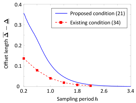
Figure 3: Allowable offset length $\overline{\Delta}-\underline{\Delta}$ versus sampling period $h$.

V Exact Bound on Offsets for First-order Systems

In this section, the bounds on the clock offset that were obtained for LTI controllers (from Theorems V.1 and IV.4) are compared with the exact bound that would be allowed if we restricted our attention to a time-invariant static output feedback controller, and with an offset range that gives a sufficient condition for the existence of a time-varying 2-periodic static output feedback controller. We also derive a bound obtained using standard robust control tools, regarding the clock offset as an additive uncertainty.

In this section, the plant class is restricted to scalar systems, and we reduce the necessary and sufficient condition for stabilizability in Theorem IV.1 to a computationally verifiable one, which gives an explicit formula for the exact bound on the clock offset that LTI controllers can allow.

Consider an unstable scalar plant: $\dot{x}=ax+bu$ with $a>0$. If $a<0$, the stabilization problem is trivial because a zero control input $u(t)=0$ leads to the stability of the closed-loop system. So in the reminder o this section, we will focus our attention to the case $a>0$. The case $a=0$ will be addressed separately later.

Solving explicitly the integrals that appear in (6), the extended system (5) is given by

$$\xi_{k+1} =\begin{bmatrix}-\lambda\theta&-\lambda\theta\\ \lambda(1+\theta)&\lambda(1+\theta)\end{bmatrix}\xi_{k}+\frac{b}{a}\begin{bmatrix}-\lambda\theta\\ \lambda(1+\theta)-1\end{bmatrix}u_{k}$$

$$y_{k} =\begin{bmatrix}0&1\end{bmatrix}\xi_{k},$$ (31)

where $\lambda:=e^{ah}$ and $\theta:=e^{-a\Delta}-1.$ In what follows, we take $b/a=1$ for simplicity of notation, because stabilizability does not depend on the value of this ratio.

The extended system (31) is stabilizable and detectable except for $\theta=-1$, at which point the system loses detectability. Since $\theta=e^{-a\Delta}-1$, it follows that

$$\Delta\in[\underline{\Delta},\overline{\Delta}]~{}~{}\Leftrightarrow~{}~{}\theta\in[e^{-a\overline{\Delta}}-1,e^{-a\underline{\Delta}}-1]=:S.$$ (32)

We have from Assumption II.2 that $-h<\Delta<h$, and hence the set $S$ on $\theta$ is a subset of

$$(e^{-ah}-1,e^{ah}-1)=:S_{\max}.$$ (33)

As in Section 3, taking the Z-transform of (31) and then mapping $z\mapsto 1/z$, we obtain the transfer function $P_{\theta}$:

$$P_{\theta}(z)=\frac{(\lambda-1)z}{1-\lambda z}-\theta\frac{\lambda z(z-1)}{1-\lambda z}\quad(\theta\in S\subset S_{\max}).$$ (34)

The system (34) belongs to a class of the so-called interval systems. The stabilization of general interval systems has been studied, e.g., in [14, 27]. Here we shall develop a new approach based on Theorem IV.1.

V-A Main result for scalar plants

The following theorem gives the exact bound on the clock offset for scalar systems:

Theorem V.1

Define $\lambda:=e^{ah}$ and $\theta:=e^{-a\Delta}-1$. Let $\underline{\theta}<0<\overline{\theta}$ and consider the set $S$ in (32) of the form $S=[\underline{\theta},\overline{\theta}]\subset S_{\max}$. There exists a controller that stabilizes $P_{\theta}$ in (34) for all $\theta\in S$, that is, there exists $Q\in\mathcal{RH}^{\infty}$ satisfying (18) for all $\theta\in S$ if and only if

$$(\lambda-1)^{2}\overline{\theta}-(\lambda+1)^{2}\underline{\theta}<4\lambda.$$ (35)

In particular, if $-\underline{\theta}=\overline{\theta}$, then (35) is equivalent to

$$\overline{\theta}<\frac{2\lambda}{\lambda^{2}+1}.$$ (36)

Furthermore, define a conformal mapping $\phi$ from $\mathbb{G}:=\mathbb{C}\setminus\{(-\infty,1/\underline{\theta}]\cup[1/\overline{\theta},\infty)\}$ to $\mathbb{D}$ by

$$\phi:~{}\mathbb{G}\to\mathbb{D}:~{}s\mapsto\frac{1-\sqrt{(1-\overline{\theta}s)/(1-\underline{\theta}s)}}{1+\sqrt{(1-\overline{\theta}s)/(1-\underline{\theta}s)}}.$$ (37)

If (35) holds, then a finite-dimensional stabilizing controller $C$ is given by

$$C:=\frac{X_{0}+D_{0}Q}{Y_{0}-N_{0}Q},\qquad Q:=\frac{\phi^{-1}\circ g-T_{1}}{T_{2}},$$

where the $\mathcal{RH}^{\infty}$ functions $N_{0}$, $D_{0}$, $X_{0}$, $Y_{0}$, $T_{1}$, and $T_{2}$ are defined by

$$N_{0}(z):=\frac{(\lambda-1)z}{z-c},\qquad D_{0}(z):=\frac{1-\lambda z}{z-c}$$

$$X_{0}(z):=\frac{1-c\lambda}{\lambda-1},\qquad Y_{0}(z):=-c$$ (38)

$$T_{1}(z):=\lambda\frac{1-c\lambda}{\lambda-1}\frac{z(z-1)}{z-c},~{}T_{2}(z):=\lambda\frac{z(z-1)(1-\lambda z)}{(z-c)^{2}}.$$

for any arbitrarily fixed $c\in\mathbb{C}$ with $|c|>1$, and any rational function $g:~{}\bar{\mathbb{D}}\to\mathbb{D}$ that satisfies the interpolation conditions $g(0)=\phi(0)$, $g(1)=\phi(0)$, and $g(1/\lambda)=\phi(-1)$. Such a function $g$ always exists if (35) holds.

Proof: See Section 4.2.  ∎

Remark V.2

The rational function $g$ in Theorem V.1 can be obtained from the Schur-Nevanlinna algorithm; see, e.g., [20, 37].

Remark V.3

Since the inverse mapping $\phi^{-1}$ is given by the following rational function:

$$\phi^{-1}(s)=\frac{4s}{\overline{\theta}(s+1)^{2}-\underline{\theta}(s-1)^{2}},$$ (39)

the stabilizing controller $C$ is finite dimensional for a rational function $g$.

If we change the offset variable from $\theta=e^{-a\Delta}-1$ to $\Delta$, then (32) and (35) give the maximum length of the offset interval $[\underline{\Delta},\overline{\Delta}]$ allowed by an LTI controller.

Corollary V.4

Assume $-h<\underline{\Delta}<0<\overline{\Delta}<h$. There exists a controller that stabilizes the extended system (31) for all $\Delta\in[\underline{\Delta},\overline{\Delta}]$ if and only if

$$\overline{\Delta}-\underline{\Delta}<\frac{2\left(\log(e^{ah}+1)-\log(e^{ah}-1)\right)}{a}.$$ (40)

Proof: See Section 4.2.  ∎

Remark V.5

In the case $a=0$, the extended system $P_{\Delta}$ is given by

$$P_{\Delta}(z)=\frac{hz}{1-z}-\Delta z.$$

Similarly to the case $a>0$, one can show that there exists a controller stabilizing $P_{\Delta}$ for all $\Delta\in(-h,h)$. This result is consistent with that in the case when $a\to 0$ in Corollary V.4, but we omit the proof for brevity.

Example V.6

Consider a scalar plant with unstable pole $a=1$. In Fig. 4, we plot the maximum length of the offset interval $(\underline{\Delta},\overline{\Delta})$ versus the ZOH-update period $h$. The solid line is the maximum length $\overline{\Delta}-\underline{\Delta}$ and the vertical dotted lines indicate $h=h_{0}:=(\log(1+\sqrt{2}))/a$. If $h<h_{0}$, then the restriction $-h<\underline{\Delta}<\overline{\Delta}<h$ arising from Assumption II.2 gives the bound $\overline{\Delta}-\underline{\Delta}<2h$. On the other hand, if $h\geq h_{0}$, then $\overline{\Delta}-\underline{\Delta}$ is bounded by (40). The maximum offset length $\overline{\Delta}-\underline{\Delta}$ exponentially decreases as $h\geq h_{0}$ becomes larger.

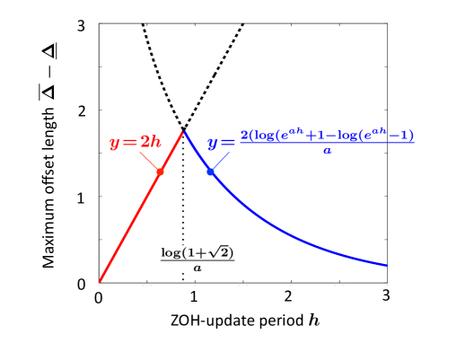
Figure 4: Maximum offset length $\overline{\Delta}-\underline{\Delta}$ versus ZOH-update period $h$ (unstable pole $a=1$): The solid line is the maximum offset length. The vertical dotted line indicates $h=(\log(1+\sqrt{2}))/a$.

V-B Proofs of Theorem V.1 and Corollary V.4

We prove Theorem V.1 by reducing the stabilization problem to a Nevanlinna-Pick interpolation problem. This reduction relies on results stated in Lemmas V.7 and V.9 have appeared in [14, 27], but we give new proofs of these results based on Theorem IV.1.

First we show that the stabilization problem is equivalent to an interpolation problem with a specified codomain:

Lemma V.7

Let $\underline{\theta}<0<\overline{\theta}$ and $S:=[\underline{\theta},\overline{\theta}]\subset S_{\max}$. There exists a controller that stabilizes $P_{\theta}$ in (34) for all $\theta\in S$, that is, there exists $Q\in\mathcal{RH}^{\infty}$ satisfying (18) for all $\theta\in S$ if and only if there exists $f\in\mathcal{RH}^{\infty}$ such that $f$ is a map from $\bar{\mathbb{D}}$ to $\mathbb{G}:=\mathbb{C}\setminus\{(-\infty,1/\underline{\theta}]\cup[1/\overline{\theta},\infty)\}$ and satisfies the interpolation conditions $f(0)=0$, $f(1)=0$, and $f(1/\lambda)=-1$.

Proof: We obtain an $\mathcal{RH}^{\infty}$ coprime factorization $P_{\theta}=N_{\theta}/D_{\theta}$ with

$$N_{\theta}(z):=\frac{(\lambda-1)z}{z-c}-\theta\frac{\lambda z(z-1)}{z-c},\quad D_{\theta}(z):=\frac{1-\lambda z}{z-c},$$ (41)

where $c$ is a fixed complex number with $|c|>1$. If we define $X_{0}$ and $Y_{0}$ as in (38), then the Bezout identity $N_{0}X_{0}+D_{0}Y_{0}=1$ holds. Hence defining $T_{1}$ and $T_{2}$ by (38), we see that $U_{\theta}+V_{\theta}Q$ in (18) satisfies

$$U_{\theta}+V_{\theta}Q=1-\theta\left(T_{1}+T_{2}Q\right)\quad(Q\in\mathcal{RH}^{\infty}).$$ (42)

Theorem IV.1 and (42) show that the plant $P_{\theta}$ is simultaneously stabilizable by a single LTI controller if and only if there exists $Q\in\mathcal{RH}^{\infty}$ such that

$$(1-\theta(T_{1}+T_{2}Q))^{-1}\in\mathcal{RH}^{\infty}\qquad(\theta\in S).$$ (43)

We have (43) if and only if $1-\theta(T_{1}+T_{2}Q)$ has no zero in $\bar{\mathbb{D}}$ for all $\theta\in S$, that is, $T_{1}(z)+T_{2}(z)Q(z)\in\mathbb{G}$ for all $z\in\bar{\mathbb{D}}$.

It is now enough to show that $G\in\mathcal{RH}^{\infty}$ if and only if $f:=T_{1}+T_{2}Q$ satisfies $f\in\mathcal{RH}^{\infty}$ and the interpolation conditions in the lemma.

Suppose that $Q\in\mathcal{RH}^{\infty}$. Since $T_{1},T_{2}\in\mathcal{RH}^{\infty}$, we have $f=T_{1}+T_{2}Q\in\mathcal{RH}^{\infty}.$ Moreover, since the unstable zeros of $T_{2}$ are $0$, $1$, and $1/\lambda$ and since $Q$ has no unstable poles, it follows that $f(0)=T_{1}(0)=0$, $f(1)=T_{1}(1)=0$, and $f(1/\lambda)=T_{1}(1/\lambda)=-1$.

Conversely, let $f\in\mathcal{RH}^{\infty}$ satisfy $f(0)=0$, $f(1)=0$, and $f(1/\lambda)=-1$. If we define

$$Q:=\frac{f-T_{1}}{T_{2}},$$ (44)

then $Q$ belongs to $\mathcal{RH}^{\infty}$. Assume, to get a contradiction, that $Q\not\in\mathcal{RH}^{\infty}$. Since

$$T_{2}Q=f-T_{1}\in\mathcal{RH}^{\infty},$$ (45)

it follows that $Q$ has some unstable poles that are zeros of $T_{2}$ in $\bar{\mathbb{D}}$. Let $p_{0}$ be one of the poles. Since $T_{2}$ has only simple zeros in $\bar{\mathbb{D}}$, it follows that $(T_{2}Q)(p_{0})\not=0$. The interpolation conditions of $f$ lead to $f(p_{0})-T_{1}(p_{0})=0$, which contradicts the equality in (45).  ∎

From Lemma V.7, it suffices to study the following interpolation problem for stabilizability:

Problem V.8

Let $z_{1},\dots,z_{n}$ be distinct points in $\bar{\mathbb{D}}$ and let $w_{1},\dots,w_{n}$ belong to $\mathbb{G}:=\mathbb{C}\setminus\{(-\infty,1/\underline{\theta}]\cup[1/\overline{\theta},\infty)\}$. Find a function $f\in\mathcal{RH}^{\infty}$ such that

$$f:~{}\bar{\mathbb{D}}\to\mathbb{G}\text{~{}~{}~{}and~{}~{}~{}}f(z_{i})=w_{i}\quad(i=1,\dots,n).$$ (46)

We solve Problem V.8 by reducing it to the Nevanlinna-Pick interpolation. To this effect, we need a conformal map from $\mathbb{G}$ to $\mathbb{D}$. In [27], [9, Section 4.1], such a conformal map $\phi$ is given in (37).

Using the conformal map defined in (37), we see that Problem V.8 can be reduced to the Nevanlinna-Pick interpolation problem.

Lemma V.9

Problem V.8 is solvable if and only if the following Nevanlinna-Pick interpolatoin problem is solvable: Find a function $g\in\mathcal{RH}^{\infty}$ such that

$$g:~{}\bar{\mathbb{D}}\to\mathbb{D}\text{~{}~{}~{}and~{}~{}~{}}g(z_{i})=\phi(w_{i})\quad(i=1,\dots,n).$$ (47)

Proof: Let $f$ be a solution to Problem V.8, and set $g=\phi\circ f$. Then we derive the equivalence between (46) and (47). Since $\phi$ is a conformal map, we see that $f$ is holomorphic in $\bar{\mathbb{D}}$ if and only if $g$ is so.

Regarding the rationality of solutions, since $\phi^{-1}$ is given by a rational function in (39) and since $f=\phi^{-1}\circ g$, it follows that $f$ is rational for every rational solution $g$.

Conversely, $\phi\circ f$ may not be rational for a rational function $f$. However, $\phi\circ f$ is holomorpic in $\bar{\mathbb{D}}$, and hence it is an irrational solution of the Nevanlinna-Pick interpolation problem. If the Nevanlinna-Pick interpolation problem is solvable, then there exists a rational solution, which can be obtained from the Schur-Nevanlinna algorithm, e.g., in [20, 37] and the explicit formula of the solutions in [9, Sec. 2.11]. We therefore have the desired rational function $g$.  ∎

Interpolating functions and a conformal map in Lemma V.9 are illustrated by the commutative diagram in Fig. 5.

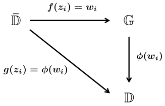
Figure 5: Interpolating functions $f,g$ and a conformal map $\phi$.

Finally we obtain the proof of Theorem V.1.

Proof of Theorem V.1: Lemmas V.7 and V.9 show that the stabilization problem for systems with clock offsets can be reduced to the Nevanlinna-Pick interpolation problem with a boundary condition; see, e.g., [9, Sec. 2.11] for the interpolation problem. We therefore obtain a necessary and sufficient condition based on the positive definiteness of the associated Pick matrix:

$$\begin{bmatrix}1&1\\ 1&\frac{1-|\phi(-1)|^{2}}{1-1/\lambda^{2}}\end{bmatrix}>0.$$ (48)

From the Schur complement formula, (48) is equivalent to

$$\frac{1-|\phi(-1)|^{2}}{1-1/\lambda^{2}}>1.$$ (49)

We see that (49) is

$$\lambda^{2}\left|1-\sqrt{\frac{1+\overline{\theta}}{1+\underline{\theta}}}\right|^{2}<\left|1+\sqrt{\frac{1+\overline{\theta}}{1+\underline{\theta}}}\right|^{2}.$$ (50)

Since $-1<\underline{\theta}<\overline{\theta}$, it follows that (50) is equivalent to

$$(p-1)^{2}(1+\overline{\theta})<(p+1)^{2}(1+\underline{\theta}).$$ (51)

After rearranging this, we derive (35). $\blacksquare$

Proof of Corollary V.4: Substituting $\underline{\theta}=e^{-a\overline{\Delta}}-1$ and $\overline{\theta}=e^{-a\underline{\Delta}}-1$ into (51), we obtain

$$(\lambda-1)^{2}e^{-a\underline{\Delta}}<(\lambda+1)^{2}e^{-a\overline{\Delta}},$$

and hence

$$e^{a(\overline{\Delta}-\underline{\Delta})}<\left(\frac{\lambda+1}{\lambda-1}\right)^{2}.$$

Taking the logarithm function of both sides gives the desired conclusion. $\blacksquare$

V-C Comparison with time-invariant/2-periodic static controllers

The proposition below gives the exact bound on the clock offset that could be obtained using a static stabilizer for a scalar plant.

Proposition V.10

Consider the extended system (31). Define $\lambda:=e^{ah}$, $\theta:=e^{-a\Delta}-1$, and $S_{\max}$ as in (33). There exists a static output feedback controller $u_{k}=-Ky_{k}$ that achieves $\lim_{k\to\infty}\xi_{k}=0$ for every $\theta\in S\subset S_{\max}$ if and only if

$$S\subset\left(-\frac{1}{\lambda},~{}\frac{1}{\lambda}\right).$$ (52)

Proof: Without loss of generality, we assume that $b/a=1$. Introducing the static controller

$$u_{k}=-K\begin{bmatrix}0&1\end{bmatrix}\xi_{k}$$

into the extended system (31), we have

$$\xi_{k+1}=\left[\begin{array}[]{cc}-\lambda\theta&-\lambda\theta(1-K)\\ \lambda(1+\theta)&\lambda(1+\theta)(1-K)+K\end{array}\right]\xi_{k}.$$ (55)

From the Jury stability criterion, the above system is stable if and only if the following three inequalities hold:

$$(\lambda-1)(K-1) >0$$ (56)

$$\lambda\theta K+1 >0$$ (57)

$$2\lambda\theta K+(\lambda-1)K-\lambda-1 <0.$$ (58)

From (56) and $\lambda>1$, we have

$$K>1.$$ (59)

Therefore (57) and (58) give a lower and upper bound on $\theta$, respectively:

$$\theta>-\frac{1}{\lambda K},\quad\theta<\frac{p+1}{2\lambda K}-\frac{\lambda-1}{2\lambda}.$$ (60)

Notice that the lower (upper) bound in (60) is increasing (decreasing) with respect to $K$. Hence these bounds take the inifimum and the supremum under (59) when $K\to 1$, and

$$\lim_{K\to 1}\left(-\frac{1}{\lambda K}\right)=-\frac{1}{\lambda},~{}~{}\lim_{K\to 1}\left(\frac{p+1}{2\lambda K}-\frac{\lambda-1}{2\lambda}\right)=\frac{1}{\lambda}.$$

Thus, there exists a static controller $K$ that stabilizes the extended system (31) for all $\theta\in S$ if and only if $S$ satisfies (52).  ∎

The next result provides a sufficient condition on the offset range $(\underline{\theta},\overline{\theta})$ for the existence of time-varying 2-periodic controllers that stabilize the extended system (31).

Proposition V.11

Consider the extended system (31). Define $\lambda:=e^{ah}$, $\theta:=e^{-A\Delta}-1$, and $S_{\max}$ as in (33). There exists a 2-periodic static controller

$$\begin{bmatrix}u_{k}\\ u_{k+1}\end{bmatrix}=-\begin{bmatrix}K_{1}&0\\ 0&K_{2}\end{bmatrix}\begin{bmatrix}y_{k}\\ y_{k+1}\end{bmatrix}$$ (61)

that achieves $\lim_{k\to\infty}\xi_{k}=0$ for every $\theta\in S\subset S_{\max}$ if

$$S\subset\left(-\frac{1}{\lambda\kappa},~{}\frac{1}{\lambda\kappa}\right),$$ (62)

where

$$\kappa:=\frac{\sqrt{\lambda^{2}+1}\sqrt{\lambda^{2}-4\sqrt{2}+5}-2\left(\sqrt{2}-1\right)\lambda}{\lambda^{2}-1}<1.$$

Proof: This is also based on the Jury stability criterion.

Without loss of generality, we assume that $b/a=1$. With the 2-periodic controller (61), the extended system (31) can be written as

$$\xi_{k+2}=\left(F^{2}-\left[\begin{array}[]{cc}FG&G\\ \end{array}\right]\left[\begin{array}[]{cc}1&0\\ -K_{2}HG&1\end{array}\right]\left[\begin{array}[]{cc}K_{1}&0\\ 0&K_{2}\end{array}\right]\left[\begin{array}[]{c}H\\ HF\end{array}\right]\right)\xi_{k},$$ (70)

where

$$F:=\left[\begin{array}[]{cc}-\lambda\theta&-\lambda\theta\\ \lambda(1+\theta)&\lambda(1+\theta)\end{array}\right],\quad G:=\left[\begin{array}[]{c}-\lambda\theta\\ \lambda(1+\theta)-1\end{array}\right],\quad H:=\left[\begin{array}[]{cc}0&1\\ \end{array}\right].$$ (76)

Denote the characteristic polynomial $\rho(\lambda)$ of the matrix in (70) by $\rho(\lambda)=\lambda^{2}+\alpha_{1}\lambda+\alpha_{0}$. The coefficients $\alpha_{0},\alpha_{1}$ are given as

$$\alpha_{0}:=\zeta p^{2}\theta^{2},$$

$$\alpha_{1}:=-\zeta\lambda^{2}\theta^{2}+(2\zeta-\eta)(1-\lambda)\lambda\theta-(\zeta-\eta+1)\lambda^{2}+(2\zeta-\eta)\lambda-\zeta,$$

where $\zeta:=K_{1}K_{2}$ and $\eta:=K_{1}+K_{2}$. From the Jury stability test, we have that stability of (70) is equivalent to the following three inequalities i)–iii): i) The first condition is given by

$$1-\alpha_{0}=1-\zeta\lambda^{2}\theta^{2}>0.$$ (77)

ii) Furthermore,

$$1+\alpha_{1}+\alpha_{0} =(2\zeta-\eta)(1-\lambda)\lambda\theta-(\zeta-\eta-1)\lambda^{2}+(2\zeta-\eta)\lambda-\zeta+1$$

$$=(1-\lambda)\left\{(2\zeta-\eta)\lambda\theta+(\zeta-\eta+1)\lambda-\zeta+1\right\}>0.$$

This inequality is equivalent to the following inequalities:

$$\begin{cases}\theta<-\frac{(\zeta-\eta+1)\lambda-\zeta+1}{(2\zeta-\eta)\lambda}&\text{if }2\zeta-\eta>0\\ \zeta>1&\text{if }2\zeta-\eta=0\\ \theta>-\frac{(\zeta-\eta+1)\lambda-\zeta+1}{(2\zeta-\eta)\lambda}&\text{if }2\zeta-\eta<0.\end{cases}$$ (78)

iii) Finally,

$$1-\alpha_{1}+\alpha_{0}=2\zeta\lambda^{2}\theta^{2}+\lambda(\lambda-1)(2\zeta-\eta)\theta+(\zeta-\eta+1)\lambda^{2}-(2\zeta-\eta)\lambda+\zeta+1>0.$$ (79)

In what follows, we fix a controller, or $(\zeta,\eta)$, and then evaluate the range of permissible $\theta$ with the controller. Suppose that $\zeta>0$ and $2\zeta-\eta<0$. For such parameters $(\zeta,\eta)$, (77) and (78) are reduced to

$$-\frac{1}{\sqrt{\zeta}\lambda}<\theta<\frac{1}{\sqrt{\zeta}\lambda}$$ (80)

and

$$\theta>-\frac{(\zeta-\eta+1)\lambda-\zeta+1}{(2\zeta-\eta)\lambda},$$ (81)

respectively. Select the parameters $(\zeta,\eta)$ so that the lower bounds on $\theta$ in (80) and (81) coincide with each other. That is, $\zeta$ and $\eta$ are chosen to satisfy the following relation:

$$\frac{1}{\sqrt{\zeta}}=\frac{(\zeta-\eta+1)\lambda-\zeta+1}{2\zeta-\eta}.$$ (82)

Moreover, we select $(\zeta,\eta)$ so that (79) holds for any $\theta\in\mathbb{R}$. This implies that

$$(\lambda-1)^{2}(2\zeta-\eta)^{2}-8\zeta\left\{(\zeta-\eta+1)p^{2}-(2\zeta-\eta)\lambda+\zeta+1\right\}<0.$$ (83)

With the above class of controllers, where $\zeta$ and $\eta$ satisfy $\zeta>0$, $2\zeta-\eta<0$, (82), and (83), the conditions (77)–(79) for stability hold if and only if (80) follows. We will show that $\zeta$ and $\eta$ satisfy $\zeta>0$, $2\zeta-\eta<0$, (82), and (83) if and only if

$$\zeta\in(\kappa^{2},1),$$ (84)

$$\eta=\frac{\sqrt{\zeta}\left\{(\lambda-1)\zeta-2\sqrt{\zeta}+\lambda+1\right\}}{\sqrt{\zeta}\lambda-1},$$ (85)

where $\kappa$ is defined in (V.11). We then analyze the bounds on $\theta$ followed by (80) when the controller belongs the class characterized by (84) and (85).

The equation (85) is obtained from (82) with the fact that $\sqrt{\zeta}\lambda-1\neq 0$.

We now aim to show (84). Substituting (82) into (83) and using $2\zeta-\eta<0$, we have that (83) is satisfied if and only if

$$\eta<2\left(\zeta+2\sqrt{\zeta}\frac{\sqrt{2}-1}{\lambda-1}\right).$$ (86)

From (85) and (86), $\zeta$ satisfies

$$\frac{(\sqrt{\zeta}-\kappa)(\sqrt{\zeta}-\kappa^{\prime})}{\sqrt{\zeta}\lambda-1}>0,$$ (87)

where $\kappa^{\prime}$ is given as

$$\kappa^{\prime}:=\frac{-\sqrt{\lambda^{2}+1}\sqrt{\lambda^{2}-4\sqrt{2}+5}-2(\sqrt{2}-1)\lambda}{\lambda^{2}-1}.$$

Note that $\sqrt{\zeta}-\kappa^{\prime}>0$ from $\lambda>1$. Thus, from (87), $\zeta$ satisfies one of the following two cases: i) $\sqrt{\zeta}>1/\lambda$ and $\sqrt{\zeta}>\kappa$, or ii) $\sqrt{\zeta}<1/\lambda$ and $\sqrt{\zeta}<\kappa$. A routine calculation shows that $\kappa>1/\lambda$. Thus, i) is reduced to $\sqrt{\zeta}>\kappa$ and ii) is to $\sqrt{\zeta}<1/\lambda$. On the other hand, from $2\zeta-\eta<0$ and (85), it follows that $\sqrt{\zeta}>1/\lambda$ and $\zeta<1$. Therefore, we arrive at (84).

Conversely, (84) implies that $\zeta>0$. Moreover, from (85), we have (82) and

$$2\zeta-\eta=\frac{\sqrt{\zeta}(\zeta-1)(\lambda+1)}{\sqrt{\zeta}\lambda-1}.$$

The right-hand side is negative by (84) and the fact $\kappa>1/\lambda$. Note also that (83) holds if $\zeta$ and $\eta$ are taken as (84) and (85).

Finally, taking the supremum and the infimum of the upper bound and the lower bound on $\theta$ in (80) over (84), we conclude the proof.  ∎

We are now in a position to compare the bounds (36), (52), and (62). For all $\lambda=e^{ah}>1$, a routine calculation shows that

$$\frac{1}{\lambda}<\frac{1}{\lambda\kappa}<\frac{2\lambda}{\lambda^{2}+1}.$$ (88)

As expected, the offset condition (52) for time-invariant static controllers results in the smallest range for values of $\theta=e^{-a\Delta}-1$ because the set of all time-invariant static controllers is a subset of the class of LTI controllers and that of 2-periodic static controllers in (61). On the other hand, 2-periodic static stabilizers do not belong to the class of LTI controllers, and vice versa. The second inequality in (88) always holds for all $\lambda>1$, but the bound (88) is a sufficient condition. In order to compare the ability to robustly stabilize the closed loop of 2-periodic static controllers versus LTI controllers, we need to do a brute-force computation for the exact bound on clock offset that would be allowed by a 2-periodic static controller.

Example V.12

Consider a scalar plant with ZOH-update period $h=1$. Fig. 6 shows the maximum offset lengths $\overline{\Delta}-\underline{\Delta}$ allowed by LTI stabilizers and static ones, which are obtained by Theorem V.1 and Proposition V.10, respectively. The figure also gives a lower bound on the maximum offset length obtained using 2-periodic static stabilizers, which is derived from Proposition V.11. All lines decreases exponentially as the unstable pole $a$ grows to $\infty$. If the unstable pole $a$ is smaller than 0.9, then Assumption II.2 gives the bound $\overline{\Delta}-\underline{\Delta}<2h=2$. We also observe that LTI controllers double the robustness with respect to that achieved by time-invariant static controllers. For example, for the unstable pole $a=1$, the maximum offset length by LTI controllers is $\overline{\Delta}-\underline{\Delta}=1.544$, whereas that by time-invariant static controllers is $\overline{\Delta}-\underline{\Delta}=0.7719$.

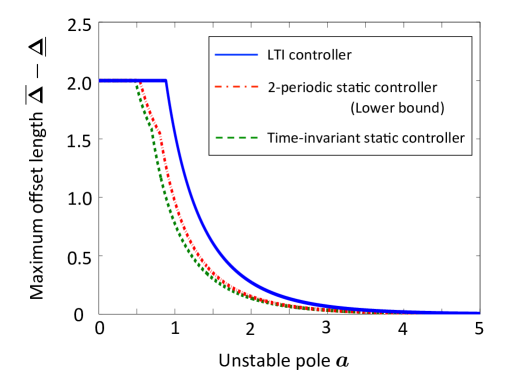
Figure 6: Comparison among the maximum offset length $\overline{\Delta}-\underline{\Delta}$ obtained using each class of controllers ($h=1$): The solid (dashed) line is the exact bound on the maximum offset length allowed by LTI (time-invariant static) controllers. The dashed-dotted line is a lower bound on the maximum offset length by 2-periodic static controllers.

V-D Conservativeness due to the small gain theorem

The sufficient condition in Theorem IV.4 with

$$L(z):=\frac{\lambda z(z-1)}{z-c},\qquad R(\theta):=\theta\qquad(c\in\mathbb{C},~{}|c|>1)$$

in (20), shows that there exists a controller stabilizing $P_{\theta}$ for all $\theta\in(-1/\lambda,1/\lambda)$. This bound of $\theta$ is the same as that was obtained in (52) for a static controller, which shows that the use of the small gain theorem is as conservative as the restriction of controllers to static gains.

This conservativeness arises from the codomain of interpolating functions. For simplicity, let the offset bound $[\underline{\theta},\overline{\theta}]=[-1,1]$. In Theorem IV.4, the stabilization problem we consider is equivalent to finding $f:\bar{\mathbb{D}}\to\mathbb{D}$ satisfying $f(0)=0$, $f(1)=0$, $f(1/\lambda)=-1$. Recall that a necessary and sufficient condition for stabilization in Lemma V.7 is the existence of a function $f:\bar{\mathbb{D}}\to\mathbb{G}=\mathbb{C}\setminus\{(-\infty,1]\cup[1,\infty)\}$ satisfying the same interpolation conditions. The difference between the codomains $\mathbb{D}$ and $\mathbb{G}$ leads to conservativeness in the stabilization analysis.

V-E Regarding a clock offset as an additive uncertainty

The transfer function $P_{\theta}$ in (34) can be viewed as a perturbation of the nominal transfer function $P_{0}=(\lambda-1)z/(1-\lambda z)$ by the following additive uncertainty:

$$P_{\theta}(z)-P_{0}(z)=m(z)r_{\theta}(z)$$

where

$$m(z):=\frac{z(\lambda-z)}{1-\lambda z},\quad r_{\theta}(z):=\frac{\theta\lambda(z-1)}{\lambda-z}.$$

Since $|m(e^{j\omega})|=1$, it follows that

$$|P_{\theta}(e^{j\omega})-P_{0}(e^{j\omega})|\leq|W_{\overline{\theta}}(e^{j\omega})|$$

for all $\omega\in[0,2\pi]$ and $\theta\in[-\overline{\theta},\overline{\theta}]$ with $\overline{\theta}>0$. Hence, as shown in [9, Sec. 3.5], there exists a controller stabilizing $P_{\theta}$ for all $\theta\in[-\overline{\theta},\overline{\theta}]$ if $\overline{\theta}$ satisfies

$$\left\|W_{\overline{\theta}}(X_{0}+QD_{0})\right\|_{\infty}<1$$ (89)

for some $Q\in\mathcal{RH}^{\infty}$, where the $\mathcal{RH}^{\infty}$ functions $X_{0}$ and $D_{0}$ are part of the coprime factorization $P_{0}=N_{0}/D_{0}$ satisfying the Bezout identity $N_{0}X_{0}+D_{0}Y_{0}=1$. Reducing the problem of finding $Q\in\mathcal{RH}^{\infty}$ with (89) to the Nevanlina-Pick interpolation problem as in [9, Sec. 4.3], we see that $\overline{\theta}$ satisfies (89) for some $Q\in\mathcal{RH}^{\infty}$ if and only if $\overline{\theta}<1/\lambda.$

This bound derived from the classical approach of $\mathcal{H}^{\infty}$ robust control turns out to also coincide with the one in (52) obtained for a static controller. This shows that the classical $\mathcal{H}^{\infty}$ robust control approach uses an unnecessarily large class of parametric uncertainty. In conjunction with the observation in Section 5.2, this discussion implies that the use of the small gain theorem, the over-approximation of a offset uncertainty by an $\mathcal{H}^{\infty}$-additive uncertainty, and the restriction of controllers to static gains have the same level of conservativeness for scalar plants.

VI Concluding Remarks

We studied the problem of stabilizing systems in which the sensor and the controller have a constant clock offset. We formulated the problem as the stabilization problem for systems with parametric uncertainty. For multi-input systems, we derived a sufficient condition that is numerically testable, based on the results of simultaneous stabilization. For first-order systems, we obtained the maximum offset length that can be allowed by an LTI controller. However, a full investigation of the problem for general-order systems and systems with model uncertainty is still an open area for future research.

References

• [1] Precision Clock Synchronization Protocol for Networked Measurement and Control Systems. IEC 61588(E):2004–IEEE Std. 1588(E), 2002.
• [2] V. Blondel, G. Campion, and M. Gevers. A sufficient condition for simultaneous stabilization. IEEE Trans. Automat. Control, 38:1264–1266, 1993.
• [3] C. Briat. Convex conditions for robust stability analysis and stabilization of linear aperiodic impulsive and sampled-data systems under dwell-time constraints. Automatica, 49:3449–357, 2013.
• [4] C. Briat and A. Seuret. Convex dwell-time characterizations for uncertain linear impulsive systems. IEEE Trans. Automat. Control, 57:3241–3246, 2012.
• [5] M. Cantoni, U. T. Jönsson, and C.-K. Kao. Robustness analysis for feedback interconnections of distributed systems via integral quadratic constraints. IEEE Trans. Automat. Control, 57:302–317, 2012.
• [6] M. C. de Oliveira, J. Bernussou, and J. C. Geromel. A new discrete-time robust stability condition. Systems Control Lett., 37:261–265, 1999.
• [7] M. C. F. Donkers, W. P. M. H. Heemels, N. van de Wouw, and L. Hetel. Stability analysis of networked control systems using a switched linear systems approach. IEEE Trans. Automat. Control, 56:2101–2115, 2011.
• [8] J. C. Doyle and G. Stein. Multivariable feedback design: Concepts for a classical/modern synthesis. IEEE Trans. Automat. Control, 26:4–16, 1981.
• [9] C. Foiaş, H. Özbay, and A. Tannenbaum. Robust Control of Infinite Dimensional Systems: Frequency Domain Methods. London: Springer, 1996.
• [10] N. M. Freris, S. R. Graham, and P. R. Kumar. Fundamental limits on synchronizing clocks over network. IEEE Trans. Automat. Control, 56:1352–1364, 2011.
• [11] E. Fridman, A. Seuret, and J.-P. Richard. Robust sampled-data stabilization of linear systems: An input delay approach. Automatica, 40:1441–1446, 2004.
• [12] H. Fujioka. A discrete-time approach to stability analysis of systems with aperiodic sample-and-hold devices. IEEE Trans. Automat. Control, 54:2440–2445, 2009.
• [13] E. Garcia, P. J. Antsaklis, and A. Montestruque. Model-Based Control of Networked Systems. Springer, 2014.
• [14] B. K. Ghosh. An approach to simultaneous system design. Part II: Nonswitching gain and dynamic feedback compensation by algebraic geometric methods. SIAM J. Control Optim., 26:919–963, 1988.
• [15] S. Graham and P. R. Kumar. Time in general-purpose control systems: The Control Time Protocol and an experimental evaluation. In Proc. 43rd IEEE CDC, 2004.
• [16] J. He, P. Cheng, L. Shi, C. Chen, and Y. Sun. Time synchronization in WSNs: A maximum-value-based consensus approach. IEEE Trans. Automat. Control, 59:660–675, 2014.
• [17] J. P. Hespanha, P. Naghshtabrizi, and Y. Xu. A survey of recent results in networked control systems. Proc. IEEE, 95:138–162, 2007.
• [18] L. Hetel, C. Fiter, H. Omran, A. Seuret, E. Fridman, J.-P. Richard, and S.-I. Niculescu. Recent developments on the stability of systems with aperiodic sampling: An overview. Automatica, 76:309–335, 2017.
• [19] X. Jiang, J. Zhang, J. J. Harding, B. J. Makela, and A. D. Domíngues-García. Spoofing GPS receiver clock offset of phasor measurement units. IEEE Trans. Power Systems, 28:3253–3262, 2013.
• [20] L. A. Luxemburg and P. R. Brown. The scalar Nevanlinna-Pick interpolation problem with boundary conditions. J. Comput. Appl. Math., 235:2615–2625, 2011.
• [21] H. Maeda and M. Vidyasagar. Some results on simultaneous stabilization. Systems Control Lett., 5:205–208, 1984.
• [22] L. Mirkin. Some remarks on the use of time-varying delay to model sample-and-hold circuits. IEEE Trans. Automat. Control, 52:1109–1112, 2007.
• [23] P. Naghshtabrizi, J. P. Hespanha, and A. R. Teel. Stability of delay impulsive systems with application to networked control systems. Trans. Inst. Meas. Control, 32:511–528, 2010.
• [24] Y. Nakamura, K. Hirata, and K. Sugimoto. Synchronization of multiple plants over networks via switching observer with time-stamp information. In Proc. SICE Annu. Conf., 2008.
• [25] H. Oishi, Y. Fujioka. Stability and stabilization of aperiodic sampled-data control systems using robust linear matrix inequalities. Automatica, 46:1327–1333, 2010.
• [26] K. Okano, M. Wakaiki, and J. P. Hespanha. Real-time control under clock offsets between sensors and controllers. In Proc. HSCC’15, 2015.
• [27] A. W. Olbrot and M. Nikodem. Robust stabilization: Some extensions of the gain margin maximization problem. IEEE Trans. Automat. Control, 39:652–657, 1994.
• [28] I.-K. Rhee, J. Lee, J. Kim, E. Serpedin, and Y.-C. Wu. Clock synchronization in wireless sensor networks: An overview. Sensors, 9:56–85, 2009.
• [29] H. H Rosenbrock. Computer-Aided Control System Design. New York: Academic Press, 1974.
• [30] H.-B. Shi and L. Qi. Static output feedback simultaneous stabilisation via coordinates transformations with free variables. IET Control Theory Appl., 3:1051–1058, 2009.
• [31] H. U. Ünal and A. İftar. A small gain theorem for systems with non-causal subsystems. Automatica, 44:2950–2953, 2008.
• [32] M. Vidyasagar. Control System Synthesis: A Factorization Approach. Cambridge, MA: MIT Press, 1985, Republished in Morgan & Claypool, 2011.
• [33] M. Vidyasagar and N. Viswanadham. Algebraic design techniques for reliable stabilization. IEEE Trans. Automat. Control, 27:1085–1095, 1982.
• [34] M. Wakaiki, K. Okano, and J. P. Hespanha. Control under clock offsets and actuator saturation. In Proc. 54th IEEE CDC, 2015.
• [35] M. Wakaiki, K. Okano, and J. P. Hespanha. Stabilization of networked control systems with clock offsets. In Proc. ACC’15, 2015.
• [36] M. Wakaiki, K. Okano, and J. P. Hespanha. $L^{2}$-gain analysis of systems with clock offsets. In Proc. ACC’16, 2016.
• [37] M. Wakaiki, Y. Yamamoto, and H. Özbay. Sensitivity reduction by strongly stabilizing controllers for MIMO distributed parameter systems. IEEE Trans. Automat. Control, 57:2089–2094, 2012.
• [38] Y. Xu and J. P. Hespanha. Estimation under controlled and uncontrolled communications in networked control systems. In Proc. 44th IEEE CDC, 2005.
• [39] M. Zeren and H. Özbay. On the strong stabilization and stable $H^{\infty}$-controller design problems for MIMO systems. Automatica, 36:1675–1684, 2000.
• [40] K. Zhou, J. C. Doyle, and K. Glover. Robust and Optimal Control. Prentice Hall, 1996.