Possible interpretation on the origin of four-fermion interaction

Abstract

We present a possible interpretation on the origin of the four-fermion interaction used in effective field theories. Inspired by the sharp momentum peak seen in Bose-Einstein condensate state, we incorporate the special gluon condensate effect into the gluon propagator. We then find that, if one considers hypothetic situation with the condensed gluon, the four-fermion contact interaction can arise from the first principle theory of quantum chromodynamics.

I Introduction

Quantum chromodynamics (QCD) is known to be the fundamental theory of quarks and gluons whose ultimate goal is to describe all the phenomena observed on hadrons, such as the proton and mesons. Perturbative approach in QCD works well at high energy thanks to the nature of asymptotic freedom Gross:1973id . However, it is difficult to investigate the physics at low energy where the strong coupling becomes large. Then people often use some effective models of QCD which contain nontrivial four-fermion interactions Nambu:1961tp ; Gross:1974jv .

The purpose of this letter is to discuss how this four-fermion interaction occurs from the first principle theory of quantum field theory. Motivated by the fact that the momentum have the sharp peak in a Bose-Einstein condensate of gaseous matter, we incorporate this momentum distribution into the propagator of gluons. Under the assumption, we find that the four-fermion contact interaction appears as the consequence of the condensate gluon momentum.

The paper is organized as follows. We present our motivation in Sec. II. We then show the four-fermion interaction can be derived starting from QCD in Sec. III. Section. IV gives a numerical test with gluon condensate. Then some discussion and concluding remarks are put in Secs. V and VI.

II Motivation

A Bose-Einstein condensate (BEC) is the interesting physical state of matter which can be realized at extremely low temperature, e.g., 170 nanokelvin for gas of rubidium atoms. The typical atomic scale corresponds to $\AA\sim 10^{7}$K so the temperature is indeed ultimately low. Under such the extreme circumstance, the particles involved share their phase information, then act as if they are one large quantum particle (this is the reason why mean-field approximation works well for condensed matter system). The characteristic observation on a BEC is the realization of the momentum peak shown in Fig. 1

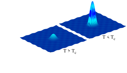
Figure 1: Schematic image of the velocity-distribution in a BEC state.

where it exhibits the image of the velocity-distribution of typical gaseous BEC matter.

We postulate, in this letter, that the gluons in hadronic state may have a similar tendency on the momentum distribution, i.e., the momentum is sharply condensed around typical QCD scale, $\mu_{\rm QCD}\sim 1{\rm fm}^{-1}(\sim 200$MeV $\sim 10^{12}$K). Note that the room temperature ($\sim 10^{2}$K) is extremely low compare to the hadron scale. We then apply this speculation by modifying the form of the gluon propagator in QCD calculation. This is the main motivation of the paper.

III Four-fermion interaction

We consider the model treatment through evaluating the partition function of QCD under the special condition mentioned in the previous section. Thereafter we try to find the relation between the original QCD Lagrangian and resulting effective model, in particular, the relation between the quark-gluon interaction and an effective four-fermion contact interaction.

III.1 QCD partition function

We first review the evaluation of the partition function in QCD whose Lagrangian density is given by

$$\mathcal{L}_{\rm QCD}=\overline{\psi}(iD_{\mu}\gamma^{\mu}-m)\psi-\frac{1}{4}F^{a}_{\mu\nu}F^{a\mu\nu},$$ (1)

where $\psi$ and $m$ are the quark field and its mass, $F_{\mu\nu}$ is the field strength tensor and $D_{\mu}$ indicates the covariant derivative defined by

$$F_{\mu\nu}^{a}=\partial_{\mu}A_{\nu}^{a}-\partial_{\nu}A_{\mu}^{a}+gf^{abc}A^{b}_{\mu}A^{c}_{\nu},$$ (2)

$$D_{\mu}=\partial_{\mu}-igA_{\mu}^{a}t^{a},$$ (3)

with the gluon field $A_{\mu}$ and the coupling constant for the strong interaction $g$. In this article, we follow the notations used in the textbook by Peskin and Schroeder Peskin:1995ev . It may be useful to separate the Lagrangian into the free and the interacting parts as

$$\mathcal{L}_{\rm QCD}=\mathcal{L}_{\rm q}^{0}+\mathcal{L}_{\rm g}^{0}+\mathcal{L}_{\rm I},$$ (4)

$$\mathcal{L}_{\rm q}^{0}=\overline{\psi}(i\partial\!\!\!/-m)\psi,$$ (5)

$$\mathcal{L}_{\rm g}^{0}=-\frac{1}{4}(\partial_{\mu}A^{a}_{\nu}-\partial_{\nu}A^{a}_{\mu})^{2},$$ (6)

$$\mathcal{L}_{\rm I}=g\overline{\psi}\gamma^{\mu}t^{a}\psi A^{a}_{\mu}-gf^{abc}(\partial_{\mu}A_{\nu}^{a})A^{\mu b}A^{\nu c}$$

$$\qquad-\frac{1}{4}g^{2}(f^{eab}A^{a}_{\mu}A^{b}_{\nu})(f^{ecd}A^{\mu c}A^{\nu d}),$$ (7)

and we also use the notation $\mathcal{L}_{0}=\mathcal{L}_{\rm q}^{0}+\mathcal{L}_{\rm g}^{0}$. This separated form helps us to write the partition function by the Taylor expansion

$$\mathcal{Z}_{\rm QCD}=\int\!\mathcal{D}\psi\int\!\mathcal{D}\!A\exp\left[i\int\mathrm{d}^{4}x\mathcal{L}_{\rm QCD}\right]$$

$$=\int\!\mathcal{D}\psi\int\!\mathcal{D}\!Ae^{i\int\mathrm{d}^{4}x{\mathcal{L}}_{0}}\sum_{n=0}^{\infty}\frac{1}{n!}\left(i\int\mathrm{d}^{4}x\mathcal{L}_{\rm I}\right)^{n}$$ (8)

where we will consider the terms up to the order of $g^{2}$ in this article.

Before proceeding the further calculations, we define the notation $\langle O\rangle$ for later convenience,

$$\langle O\rangle=\frac{\int\mathcal{D}\psi\int\mathcal{D}\!Ae^{i\int\mathrm{d}^{4}x{\mathcal{L}}_{0}}\left[O\right]}{\int\mathcal{D}\psi\int\mathcal{D}\!Ae^{i\int\mathrm{d}^{4}x{\mathcal{L}}_{0}}},$$ (9)

here Eq. (9) indicates the expectation value of $O$.

As is well known, quarks and gluons have never been observed as free particles due to non-trivial effect of the confinement, we expect the amplitudes containing the outgoing quarks and gluons vanish, namely,

$$\langle\overline{\psi}\gamma^{\mu}t^{a}\psi A^{a}_{\mu}\rangle=0,$$ (10)

$$\langle(\partial_{\mu}A_{\nu}^{a})A^{\mu b}A^{\nu c}\rangle=0.$$ (11)

Retaining non-vanishing contributions in the partition function, we have

$$\mathcal{Z}_{\rm QCD}\simeq\int\!\mathcal{D}\psi\int\!\mathcal{D}\!Ae^{i\int\mathrm{d}^{4}x{\mathcal{L}}_{0}}$$

$$\quad\times\biggl{[}1+\frac{1}{2}\left(ig\int\mathrm{d}^{4}x\overline{\psi}\gamma^{\mu}t^{a}\psi A^{a}_{\mu}\right)^{2}$$

$$\qquad+\frac{1}{2}\left(ig\int\mathrm{d}^{4}xf^{abc}(\partial_{\mu}A_{\nu}^{a})A^{\mu b}A^{\nu c}\right)^{2}$$

$$\qquad-\frac{1}{4}\left(ig^{2}\int\mathrm{d}^{4}x(f^{eab}A^{a}_{\mu}A^{b}_{\nu})(f^{ecd}A^{\mu c}A^{\nu d})\right)\biggr{]}.$$ (12)

This is the partition function of QCD at $g^{2}$ order, and we will try to consider this quantity under special circumstance in the following.

III.2 Quark sector

In this subsection, we are going to study what happens if one integrates out the gluon degree of freedom, then discuss the possible relation between original QCD interaction and the four-fermion interaction.

The term relating to the quark-gluon interaction can be evaluated by

$$\mathcal{Z}_{{\rm qq}g}=-\frac{g^{2}}{2}\int\!\mathcal{D}\psi\int\!\mathcal{D}\!Ae^{i\int\mathrm{d}^{4}x{\mathcal{L}}_{0}}$$

$$\quad\times\left(\int\mathrm{d}^{4}x\overline{\psi}_{x}\gamma^{\mu}t^{a}\psi_{x}A^{a}_{\mu x}\int\mathrm{d}^{4}y\overline{\psi}_{y}\gamma^{\nu}t^{b}\psi_{y}A^{b}_{\nu y}\right),$$ (13)

where we introduced the abbreviated notations $\psi_{x}=\psi(x)$ and $A^{a}_{\mu x}=A^{a}_{\mu}(x)$. The usual rule for the gluon propagator reads

$$\bigl{\langle}A^{a}_{\mu}(x)A^{b}_{\nu}(y)\bigr{\rangle}=\int\frac{\mathrm{d}^{4}p}{(2\pi)^{4}}\frac{-ig_{\mu\nu}\delta^{ab}}{p^{2}}e^{-ip\cdot(x-y)},$$ (14)

in the Feynman gauge $\xi=1$. Up to here, the treatment is general; we just briefly reviewed quantum field theory calculation. In the following, we will introduce some crude hypothesis.

Assuming the situation that the gluon is highly condensed and its momentum has narrow peak around $\mu_{\rm g}$ as discussed in Sec. II, we perform the following replacement,

$$\frac{1}{p^{2}}\to\frac{1}{\mu_{\rm g}^{2}}.$$ (15)

We regard the quantity $\mu_{\rm g}$ as the energy scale of the gluon. Once this brute force manipulation is allowed, we have

$$\bigl{\langle}A^{a}_{\mu}(x)A^{b}_{\nu}(y)\bigr{\rangle}=\frac{-ig_{\mu\nu}\delta^{ab}}{\mu_{\rm g}^{2}}\delta^{(4)}(x-y).$$ (16)

This becomes our Feynman rule for the gluon propagator in the present model. Substituting the above rule into Eq. (13), we obtain

$$\mathcal{Z}_{{\rm qq}g}={\mathcal{N}}_{A}\int\!\mathcal{D}\psi e^{i\int\mathrm{d}^{4}x{\mathcal{L}}_{\rm q}^{0}}$$

$$\times\left[\frac{ig^{2}}{2\mu_{\rm g}^{2}}\int\mathrm{d}^{4}x(\overline{\psi}_{x}\gamma^{\mu}t^{a}\psi_{x})(\overline{\psi}_{x}\gamma_{\mu}t^{a}\psi_{x})\right].$$ (17)

where ${\mathcal{N}}_{A}$ is the overall constant from the functional integration on gluon. Note that the integral for $y$ disappears due to the delta function $\delta^{(4)}(x-y)$, then $\psi(y)$ turns out to be $\psi(x)$ in Eq. (17). This may be regarded as the reason of contact interactions which come from the resulting delta function.

As the final step, using the approximated relation $e^{\epsilon}\simeq 1+\epsilon$, we put back the resulting term inside the exponential,

$$\mathcal{Z}_{{\rm q}} ={\mathcal{N}}_{A}\int\!\mathcal{D}\psi e^{i\int\mathrm{d}^{4}x{\mathcal{L}}_{\rm q}^{0}}$$

$$\times\exp\left[\frac{ig^{2}}{2\mu_{\rm g}^{2}}\int\mathrm{d}^{4}x(\overline{\psi}\gamma^{\mu}t^{a}\psi)(\overline{\psi}\gamma_{\mu}t^{a}\psi)\right].$$ (18)

Since there arises no confusion in the above expression we drop the suffix $x$ in $\psi_{x}(=\psi(x))$. Then we finally arrive at the form

$$\mathcal{Z}_{{\rm q}}={\mathcal{N}}_{A}\int\!\mathcal{D}\psi e^{i\int\mathrm{d}^{4}x{\mathcal{L}}_{\rm q}},$$ (19)

with

$${\mathcal{L}}_{\rm q}=\overline{\psi}(i\partial\!\!\!/-m)\psi+\frac{g^{2}}{2\mu_{\rm g}^{2}}(\overline{\psi}\gamma^{\mu}t^{a}\psi)(\overline{\psi}\gamma_{\mu}t^{a}\psi).$$ (20)

Thus we obtained the effective Lagrangian with four-fermion contact interaction.

It is interesting that the only one replacement, although it looks awful, leads the four-fermion contact interaction. We think this can be a possible interpretation on the origin of the four-fermion interaction in effective field theories.

III.3 Gluon sector

We consider the gluon energy in this subsection by evaluating the contribution of the third and fourth lines in Eq. (12).

By using our propagator, we see that the contribution

$$f^{abc}f^{def}\Bigl{\langle}(\partial^{x}_{\mu}A_{\nu x}^{a})A_{x}^{\mu b}A_{x}^{\nu c}(\partial^{y}_{\rho}A_{\lambda y}^{d})A_{y}^{\rho e}A_{y}^{\lambda f}\Bigr{\rangle}$$ (21)

from the third line in Eq. (12) vanishes, due to the property of the antisymmetric tensor $f^{abc}$. Non-zero contribution occurs from the fourth line, in which one sees

$${\mathcal{Z}}_{\rm QCD}^{(4)}=-{\mathcal{Z}}_{0}\cdot 72g^{2}i\int\mathrm{d}^{4}x\phi_{\rm g}^{2}.$$ (22)

where ${\mathcal{Z}}_{0}\equiv\int\mathcal{D}\psi\int\mathcal{D}\!Ae^{i\int\mathrm{d}^{4}x{\mathcal{L}}_{0}}$ and $\phi_{\rm g}$ is the gluon one-loop amplitude,

$$\phi_{\rm g}=\int\frac{\mathrm{d}^{4}p}{(2\pi)^{4}}\frac{-i}{\mu_{\rm g}^{2}},$$ (23)

with the propagator for the gluon field set by Eq. (15). As obviously seen from the equation, this one-loop contribution, $\phi_{\rm g}$, badly diverges, then one needs to perform the renormalization to obtain finite physical quantity.

Putting back the resulting term into the exponential as done in the fermion case using the trick ($1+\epsilon\to e^{\epsilon}$), we obtain the following form

$${\mathcal{L}}_{\rm g}=-\frac{1}{4}(\partial_{\mu}A^{a}_{\nu}-\partial_{\nu}A^{a}_{\mu})^{2}-72g^{2}\phi_{\rm g}^{2}.$$ (24)

This is our effective Lagrangian for the gluon sector. We will not make further analyses on this form because our focus here is to construct the four-fermion quark model.

IV Numerical test

We have calculated the effective Lagrangian in the previous section, and it may be now ready for performing the actual numerical analyses.

As a simple test, we draw the phase diagram of the chiral phase transition on temperature and chemical potential plane. The model with the form Eq. (20) is the NJL-type model, and we just follow the prescriptions in preceding analyses Klevansky:1992qe ; Hatsuda:1994pi . Applying the mean-field approximation after the Fiertz transformation to Eq. (20) in the massless two-flavor version, we have

$${\mathcal{L}}=\overline{\psi}(i\partial\!\!\!/-M)\psi-\frac{2g^{2}}{9\mu_{\rm g}^{2}}\phi_{\psi}^{2},$$ (25)

where $M$ is the constituent (dynamical) quark mass $M=-2G\phi_{\psi}$ with $G=2g^{2}/(9\mu_{\rm g}^{2})$, and $\phi_{\psi}$ represents the chiral condensate,

$$\phi_{\psi}=\langle\overline{\psi}\psi\rangle=-{\rm tr}\int\frac{\mathrm{d}^{4}q}{(2\pi)^{4}}\frac{i}{q\!\!\!/-M}.$$ (26)

In the above expression, the trace runs for the color, flavor and spinor spaces, then the relation $\langle\overline{\psi}\psi\rangle=\langle\bar{u}u+\bar{d}d\rangle$, namely, $\phi_{\psi}=\phi_{u}+\phi_{d}$ holds. Here we treat $\mu_{\rm g}$ as the model parameter being some constant, then we no longer have the renormalizability of the original theory.

The evaluation of the effective potential at finite temperature ($T$) and chemical potential ($\mu$) is straightforward due to the mean-field approximation, and we have

$${\mathcal{V}}=\frac{2g^{2}}{9\mu_{\rm g}^{2}}\phi_{\psi}^{2}-12\int\frac{\mathrm{d}^{3}q}{(2\pi)^{3}}\left[E+T\sum_{\pm}\ln\left(1+e^{-\beta E^{\pm}}\right)\right],$$ (27)

with $E^{\pm}=E\pm\mu$, $E=\sqrt{q^{2}+M^{2}}$ and $\beta=1/T$ Huang:2004ik . Once we have the effective potential, the expectation value of the order parameter, $\phi_{\psi}$, can be determined by the gap equation, $\partial\mathcal{V}/(\partial\phi_{\psi})=0$, corresponding to the stational condition of the effective potential.

The remaining preparation for the numerical analysis is the parameter fitting. As usual, we introduce the three-momentum cutoff, $\Lambda$, to obtain the finite contribution from the loop integral. Thereafter the present model contains three parameters, the strong coupling $g$, the three momentum cutoff $\Lambda$ and the gluon energy scale $\mu_{\rm g}$. Here we chose, $\Lambda=623$MeV and $g=1.27$, then test various values of $\mu_{\rm g}$. The above parameters are chosen so that the model reproduces the numbers, $M=335$MeV and $f_{\pi}=92$MeV for $\mu_{\rm g}=250$MeV.

Figure 2 displays the numerical results of the phase diagram on the chiral phase transition.

Figure 2: $\mu_{\rm g}$ dependence on the phase diagram.

One sees that the region of the broken phase shrinks with increasing $\mu_{\rm g}$. This can easily be understood, because the effective coupling strength, $G(\mu_{\rm g}^{2})=2g^{2}/(9\mu_{\rm g}^{2})$, becomes weak when $\mu_{\rm g}^{2}$ is larger. Observing the gluon scale dependence on the model, we think that $\mu_{\rm g}$ plays a similar role with the renormalization scale in quantum field theory.

V Other relation

It may also be worth mentioning that the relation between the Schwinger-Dyson equation (SDE) Dyson:1949ha ; Schwinger:1951ex and the NJL can be seen by a similar way. Below shows the SDE for the dynamical mass, $M(p)$,

$$M(p)=-iC_{2}g^{2}{\rm tr}\int\frac{\mathrm{d}^{4}q}{(2\pi)^{4}}\frac{-i}{k^{2}}\frac{i}{q\!\!\!/-M(q)}$$ (28)

with $C_{2}=(N_{\rm c}^{2}-1)/(2N_{\rm c})$ and $k=p-q$, where we chose the Feynman gauge and set the field strength renormalization factor to be unity in the original equation for explanation simplicity. It should be noted that the trace does not include the flavor space in Eq. (28) contrary to Eq. (26). Performing the replacement, $1/k^{2}=-1/\mu_{\rm g}^{2}$, we see

$$M(p)=C_{2}\frac{g^{2}}{\mu_{\rm g}^{2}}{\rm tr}\int\frac{\mathrm{d}^{4}q}{(2\pi)^{4}}\frac{i}{q\!\!\!/-M(q)}.$$ (29)

Further, if one drops the momentum dependence on $M(p)\to M$ and recalls the relation $M_{u}=-4G\phi_{u}$ for up quark,

$$\phi_{u}=-\frac{9C_{2}}{8}{\rm tr}\int\frac{\mathrm{d}^{4}q}{(2\pi)^{4}}\frac{i}{q\!\!\!/-M_{u}}.$$ (30)

Thus we just get the same form with the NJL gap equation. Note that if the models are numerically close under the assumption of constant $k^{2}$ and $M(p)$, the relation for the coupling strength is expected to be $g_{\rm SDE}^{2}/g_{\rm NJL}^{2}\simeq 2/3$. Although the direct comparison is difficult, practical analyses show both couplings may have similar values Roberts:1994dr .

VI Concluding remarks

We find that the frequently studied four-fermion interaction in effective models can be derived by QCD, if we employ the brute forth hypothesis shown in Eq. (15). The performed manipulation is based on the speculation that the gluon momentum may have narrow peak as seen in a BEC state in condensed matter physics. We believe that, since the simple replacement can produce the four point interaction, the treatment employed here may have some physical importance.

Since the NJL model, an effective model of QCD, is introduced by using the analogy from the Bardeen Cooper Schrieffer (BCS) theory Bardeen:1957kj , an effective theory of quantum electrodynamics (QED). Therefore, we believe that the relation between QED and the BCS theory can be read in a similar manner presented in this paper.

- (1) D. J. Gross and F. Wilczek, Phys. Rev. Lett. 30, 1343 (1973).
- (2) Y. Nambu and G. Jona-Lasinio, Phys. Rev. 122, 345 (1961); 124, 246 (1961).
- (3) D. J. Gross and A. Neveu, Phys. Rev. D 10, 3235 (1974).
- (4) M. E. Peskin and D. V. Schroeder, Reading, USA: Addison-Wesley (1995).
- (5) S. P. Klevansky, Rev. Mod. Phys. 64 (1992) 649.
- (6) T. Hatsuda and T. Kunihiro, Phys. Rept. 247 (1994) 221.
- (7) M. Huang, Int. J. Mod. Phys. E 14 (2005) 675.
- (8) F. J. Dyson, Phys. Rev. 75, 1736 (1949).
- (9) J. S. Schwinger, Proc. Nat. Acad. Sci. 37, 452 (1951).
- (10) C. D. Roberts and A. G. Williams, Prog. Part. Nucl. Phys. 33, 477 (1994).
- (11) J. Bardeen, L. N. Cooper and J. R. Schrieffer, Phys. Rev. 106, 162 (1957).