Dislocation patterning in a 2D continuum theory of dislocations

Abstract

Understanding the spontaneous emergence of dislocation patterns during plastic deformation is a long standing challenge in dislocation theory. During the past decades several phenomenological continuum models of dislocation patterning were proposed, but few of them (if any) are derived from microscopic considerations through systematic and controlled averaging procedures. In this paper we present a 2D continuum theory that is obtained by systematic averaging of the equations of motion of discrete dislocations. It is shown that in the evolution equations of the dislocation densities diffusion like terms neglected in earlier considerations play a crucial role in the length scale selection of the dislocation density fluctuations. It is also shown that the formulated continuum theory can be derived from an averaged energy functional using the framework of phase field theories. However, in order to account for the flow stress one has in that case to introduce a nontrivial dislocation mobility function, which proves to be crucial for the instability leading to patterning.

I Introduction

Shortly after the first images of dislocations were seen in TEM it was realized that the dislocation distribution in a deformed crystalline material is practically never homogeneous. Depending on the slip geometry, the mode of loading and the temperature, rather different pattern morphologies (e.g. cell Kawasaki and Takeuchi (1980), labyrinth Zhang et al. (2003), vein Siu and Ngan (2013) or wall Mughrabi (1983) structures) emerge. There are, however, two important feature common to all these patterns: It is almost always observed that the characteristic wavelength $\Lambda$ of the patterns is proportional to the dislocation spacing, $\Lambda\propto 1/\sqrt{\rho}$ where $\rho$ is the total dislocation density, and inversely proportional to the stress at which the patterns have formed. These relationships are commonly referred to as “law of similitude” (for a general overview see Ref. Sauzay and Kubin (2011)).

Since the early 1960s several theoretical and numerical attempts have been made to model dislocation pattern formation. The first models were based on analogies with other physical problems like spinodal decomposition Holt (1970), patterning in chemical reaction-diffusion systems Walgraef and Aifantis (1985); Pontes et al. (2006), internal energy minimization Hansen and Kuhlmann-Wilsdorf (1986), or noise-induced phase transitions Hahner (1996); Hahner and Zaiser (1999). Since, however, it is difficult to see how these models are related to the rather specific properties of dislocations (like long range scale free interactions, motion on well defined slip planes, or different types of short-range effects, etc.) they have to be considered as attempts to reproduce some phenomenological aspects of the patterns based on heuristic analogies, rather than deriving them from the physics of dislocation systems.

To identify the key ingredients responsible for the emergence of inhomogeneous dislocation patterms, discrete dislocation dynamics (DDD) simulation is a promising possibility Ghoniem and Sun (1999); Kubin and Canova (1992); Rhee et al. (1998); Gomez-Garcia et al. (2006). The major difficulty, however, is that according to experimental observations the characteristic length scale of the dislocation patterns is an order of magnitude larger than the dislocation spacing Sauzay and Kubin (2011). So, to be able to detect patterning in a DDD simulation one has to work with systems containing a large amount of dislocation lines: to see 3-5 pattern wavelengths in each spatial direction, the system size should be 30-50 times larger than $1/\sqrt{\rho}$. Especially in 3D this is a rather hard task. Although irregular clusters or veins are regularly observed in simulations Devincre, B and Kubin, LP and Lemarchand, C and Madec, R (2001); Madec, R and Devincre, B and Kubin, LP (2002); Hussein, Ahmed M. and Rao, Satish I. and Uchic, Michael D. and Dimiduk, Dennis M. and El-Awady, Jaafar A. (2015) clear evidence of the emergence of a characteristic length scale has not been published so far.

During the past decade continuum theories of dislocations derived by rigorous homogenization of the evolution equations of individual dislocations have been proposed in 2D single slip Groma (1997); Zaiser et al. (2001); Groma et al. (2003, 2007, 2015) by the present authors and by Mesarovic et.al. Mesarovic et al. (2010). Later these models were extended to multiple slip by Limkumnerd and Van der Giessen Limkumnerd and Van der Giessen (2008). In order to obtain closed sets of evolution equations for the dislocation densities, assumptions about the correlation properties of dislocation systems have to be made, but there are essential differences with earlier phenomenological models: Not only can these assumptions be shown to be consistent with the fundamental scaling properties of dislocation systems Zaiser et al. (2001); Zaiser and Sandfeld (2014), but also the numerical parameters entering the theories can be deduced from DDD simulations in a systematic manner without fitting them in an ad-hoc manner to desired results. As a consequence, the models are predictive and can be directly validated by comparing their results to the outcomes of DDD simulations Groma et al. (2003); Zaiser et al. (2001); Yefimov et al. (2004); Groma et al. (2015).

Since 2D models are not able to account for several effects playing an important role in the evolution of the dislocation network, most importantly dislocation multiplication and junction formation, several 3D continuum theories have been proposed. For example Acharya Roy et al. (2007) and later on Chen et.al. Chen et al. (2013) proposed models in which the coarse grained dislocation density (Nye’s) tensor plays a central role. This tensor provides information about the distribution of ’geometrically necessary’ dislocations with excess Burgers vector. However, incipient dislocation patterns are often associated with modulations in the total density of dislocations rather than modulations of the Burgers vector content. Hence it is doubtful whether models which concentrate on the transport of excess Burgers vector only can capture patterning.

Applying statistical approaches, El-Azab El-Azab (2000) and Sedlacek et.al. Sedlacek et al. (2007); Kratochvil and Sedlacek (2008) suggested methods to handle curved dislocations, but the evolution equations obtained are valid only for quite specific situations. Considerable progress towards a generic statistical theory of dislocation motion in 3D has been made by Hochrainer et.al. Hochrainer et al. (2007, 2014); Hochrainer (2015) by deriving a theory of dislocation density transport which applies to systems of three-dimensionally curved dislocations and can represent the evolution of generic dislocation systems comprising not only ’geometrically necessary’ but also ’statistically stored’ dislocations with zero net Burgers vector. Depending on the desired accuracy, the approach of Hochrainer allows to systematically derive density-based theories of increasing complexity. Recently this work was complemented by the derivation of matching energy functionals based upon averaging the elastic energy functionals of the corresponding discrete dislocation systems Zaiser (2015). In parallel, it was demonstrated how such energy functionals can be used to derive closed-form dislocation dynamics equations which are consistent not only with thermodynamics, but also with the constraints imposed by the ways in which dislocations move in 3D Hochrainer (2016).

Concerning dislocation patterning, the general structure of continuum theories that is required for predicting dislocation patterns that are compatible with the “principle of similitude” has been recently discussed by Zaiser and Sandfeld Zaiser and Sandfeld (2014). It was argued that no other length scales except the dislocation spacing ($1/\sqrt{\rho}$) should appear in such theories - in other words, such theories ought to be scale free. In Ref.Zaiser and Sandfeld (2014) the authors also discussed a possible extension of the 2D continuum theory of Groma et.al Groma et al. (2003) leading to the instability of the homogeneous dislocation density in a deforming crystal (details are discussed below).

Some remarkable steps towards modeling pattern formation have been made by Kratochvil et.al. Kratochvil and Sedlacek (2003) and recently in a 3D mean field theory by Xia and El-Azab Xia and El-Azab (2015). In order to obtain patterns, however, in both models specific microscopic dislocation mechanisms (sweeping narrow dipoles by moving curved dislocations, or cross slip, respectively) had to be invoked. In the present paper we adopt a more minimalistic approach where we consider no other mechanisms apart from the elastic interaction of dislocation lines. We analyze in detail the properties of a 2D single slip continuum theory of dislocations that is a generalization of the theory we have proposed earlier Groma (1997); Zaiser et al. (2001); Groma et al. (2003, 2007, 2015). In the first part, the general structure of the dislocation field equations is outlined. To obtain a closed set of equations an assumption similar to the “local density approximation” often used for many-electron systems is used. After this, it is shown that the same evolution equations can be derived in a complementary manner, using the formalism of phase field theories, from a functional which expresses the energy of the dislocation system as a functional of the dislocation densities. In the last part, by linear stability analysis of the trivial solution of the field equations the mechanisms for characteristic length scale selection in dislocation patterning are discussed.

II Density based representation of a dislocation system: Linking micro- to mesoscale

Let us consider a system of $N$ parallel edge dislocations with line vectors $\vec{l}=(0,0,1)$ and Burgers vectors $\vec{b}_{\pm}=\pm(b,0,0)$. The force in the slip plane acting on a dislocation is $b\tau$ where $\tau$ is the sum of the shear stresses generated by the other dislocations, and the stress $\tau_{\rm ext}$ arising from external boundary displacements or tractions. It is commonly assumed that the velocity of a dislocation is proportional to the shear stress acting on the dislocation (over-damped dynamics) Groma (1997); Groma et al. (2003). So, the equation of the motion of the $i$th dislocation positioned in the $xy$ plane at point $\vec{r}_{i}$ is

$$\frac{dx_{i}}{dt}=M_{0}b\tau(\vec{r}_{i})=M_{0}{b_{i}}\left(\sum_{j=1,j\neq i}^{N}s_{j}\tau_{\rm ind}(\vec{r}_{i}-\vec{r}_{j})+\tau_{\rm ext}\right)$$ (1)

where $M_{0}$ is the dislocation mobility, $s_{i}=b_{i}/b=\pm 1$ is the sign of the $i$th dislocation (in the following often labeled ’+’ for $s=1$ and ’$-$’ for $s=-1$), $\tau_{\rm ext}$ is the external stress, and

$$\tau_{\rm ind}(\vec{r})=\frac{b\mu}{2\pi(1-\nu)}\frac{x(x^{2}-y^{2})}{(x^{2}+y^{2})^{2}}$$ (2)

is the shear stress generated by a dislocation in an infinite medium. Here $\mu$ is the shear modulus and $\nu$ is Poisson’s ratio.

After ensemble averaging as explained in detail elsewhere Groma (1997); Groma et al. (2003, 2007) one arrives at the following evolution equations:

$$\partial_{t}\rho_{+}(\vec{r},t)+M_{0}b\partial_{x}\left[\rho_{+}(\vec{r},t)\tau_{\rm ext}\right.$$

$$+\left.\int\left\{\rho_{++}(\vec{r},\vec{r}^{\prime},t)-\rho_{+-}(\vec{r},\vec{r}^{\prime},t)\right\}\,\tau_{\rm ind}(\vec{r}-\vec{r}^{\prime}){\rm d}^{2}r^{\prime}\right]=0,$$

$$\partial_{t}\rho_{-}(\vec{r},t)-M_{0}b\partial_{x}\left[\rho_{-}(\vec{r},t)\tau_{\rm ext}\right.$$

$$-\left.\int\left\{\rho_{--}(\vec{r},\vec{r}^{\prime},t)-\rho_{-+}(\vec{r},\vec{r}^{\prime},t)\right\}\,\tau_{\rm ind}(\vec{r}-\vec{r}^{\prime}){\rm d}^{2}r^{\prime}\right]=0$$

where $\rho_{s}(\vec{r})$ and $\rho_{s,s^{\prime}}(\vec{r},\vec{r}^{\prime})$ with $s,s^{\prime}\in\{+,-\}$ are the ensemble averaged one and two-particle dislocation density functions corresponding to the signs indicated by the subscripts. It should be mentioned that Eqs. (II,II) are exact, i.e. no assumptions have to be made to derive them, but certainly they do not represent a closed set of equations. In order to arrive at a closed set of equations one has to make some closure approximation to express the terms depending on the two particle density functions as functionals of the one particle densities (or one has to go to higher order densities.) The rest of this section is about suggesting a closure approximation consistent with discrete dislocation simulation results.

For the further considerations it is useful to introduce the pair-correlation functions $d_{ss^{\prime}}(\vec{r}_{1},\vec{r}_{2})$ defined by the relation

$$\rho_{ss^{\prime}}(\vec{r}_{1},\vec{r}_{2},t)=\rho_{s}(\vec{r}_{1})\rho_{s^{\prime}}(\vec{r}_{2})(1+d_{ss^{\prime}}(\vec{r}_{1},\vec{r}_{2}))$$ (5)

According to DDD simulations the pair-correlation functions defined above decay to zero within a few dislocation spacings Zaiser et al. (2001). As a result of this, if the total dislocation density $\rho=\rho_{+}+\rho_{-}$ varies slowly enough in space, we can assume that the correlation functions depend explicitly only on the relative coordinate $\vec{r}_{1}-\vec{r}_{2}$, see Refs. Groma et al. (2003, 2007). The direct $\vec{r}_{1}$ (or $\vec{r}_{2}$) dependence appears only through the local dislocation density, i.e.,

$$d_{ss^{\prime}}(\vec{r}_{1},\vec{r}_{2})=d_{ss^{\prime}}(\vec{r}_{1}-\vec{r}_{2},\rho(\vec{r}_{1})).$$ (6)

(Since $d_{ss^{\prime}}$ is short ranged in $\vec{r}_{1}-\vec{r}_{2}$, it does not make any difference if in the above expression $\rho(\vec{r}_{1})$ is replaced by $\rho(\vec{r}_{2})$.)

In the case of a weakly polarized dislocation arrangement where $\rho_{+}-\rho_{-}\ll\rho$, the only relevant length scale is the average dislocation spacing. So, for dimensionality reasons the $\rho$ dependence of $d_{ss^{\prime}}$ has to be of the form

$$d_{ss^{\prime}}(\vec{r}_{1},\vec{r}_{2})=d_{ss^{\prime}}((\vec{r}_{1}-\vec{r}_{2})\sqrt{\rho(\vec{r}_{1})}).$$ (7)

By substituting Eq. (5) into Eqs. (II,II) and introducing the GND dislocation density $\kappa=\rho_{+}-\rho_{-}$ one arrives at

$$\partial_{t}\rho_{+}(\vec{r},t)+M_{0}b\partial_{x}\left\{\rho_{+}\left[\tau_{\rm ext}+\tau_{\rm sc}+\tau_{+}\right]\right\}=0$$ (8)

$$\partial_{t}\rho_{-}(\vec{r},t)-M_{0}b\partial_{x}\left\{\rho_{-}\left[\tau_{\rm ext}+\tau_{\rm sc}+\tau_{-}\right]\right\}=0$$ (9)

where

$$\tau_{\rm sc}(\vec{r})=\int\tau_{\rm ind}(\vec{r}-\vec{r}^{\prime})\kappa(\vec{r}^{\prime}){\rm d}^{2}r^{\prime},$$ (10)

commonly called the “self consistent” or “mean field” stress, is a non-local functional of the GND density, whereas the stresses

$$\tau_{+}(\vec{r})=\int\left[\rho_{+}(\vec{r}^{\prime})d_{++}(\vec{r}-\vec{r}^{\prime})\right.$$ (11)

$$-\left.\rho_{-}(\vec{r}^{\prime})d_{+-}(\vec{r}-\vec{r}^{\prime})\right]\tau_{\rm ind}(\vec{r}-\vec{r}^{\prime}){\rm d}^{2}r^{\prime},$$

and

$$\tau_{-}(\vec{r})=-\int\left[\rho_{-}(\vec{r}^{\prime})d_{--}(\vec{r}-\vec{r}^{\prime})\right.$$ (12)

$$-\left.\rho_{+}(\vec{r}^{\prime})d_{-+}(\vec{r}-\vec{r}^{\prime})\right]\tau_{\rm ind}(\vec{r}-\vec{r}^{\prime}){\rm d}^{2}r^{\prime}$$

depend on dislocation-dislocation correlations. Finally let us introduce the quantities

$$\tau_{v} = \frac{\tau_{+}+\tau_{-}}{2},$$ (13)

$$\tau_{a} = \frac{\tau_{+}-\tau_{-}}{2}.$$ (14)

With these quantities Eqs. (8,9) read

$$\partial_{t}\rho_{+}(\vec{r},t)+M_{0}b\partial_{x}\left\{\rho_{+}\left[\tau_{\rm ext}+\tau_{\rm sc}+\tau_{v}+\tau_{a}\right]\right\}=0,$$ (15)

$$\partial_{t}\rho_{-}(\vec{r},t)-M_{0}b\partial_{x}\left\{\rho_{-}\left[\tau_{\rm ext}+\tau_{\rm sc}+\tau_{v}-\tau_{a}\right]\right\}=0.$$ (16)

In explicit form the stresses $\tau_{v}$ and $\tau_{a}$ are given by

$$\tau_{v}(\vec{r})= \int\left[\rho(\vec{r}^{\prime})d_{a}(\vec{r}-\vec{r}^{\prime})+\kappa(\vec{r}^{\prime})d_{s}(\vec{r}-\vec{r}^{\prime})\right]$$ (17)

$$*\tau_{\rm ind}(\vec{r}-\vec{r}^{\prime}){\rm d}^{2}r^{\prime},$$

$$\tau_{a}(\vec{r})= \int\left[\rho(\vec{r}^{\prime})d_{p}(\vec{r}-\vec{r}^{\prime})+\kappa(\vec{r}^{\prime})d_{a^{\prime}}(\vec{r}-\vec{r}^{\prime})\right]$$ (18)

$$*\tau_{\rm ind}(\vec{r}-\vec{r}^{\prime}){\rm d}^{2}r^{\prime},$$

with

$$d_{s} =\frac{1}{2}(d_{++}+d_{--}+d_{+-}+d_{-+}),$$ (19)

$$d_{p} =\frac{1}{2}(d_{++}+d_{--}-d_{+-}-d_{-+}),$$ (20)

$$d_{a} =\frac{1}{2}(d_{++}-d_{--}-d_{+-}+d_{-+}),$$ (21)

$$d_{a^{\prime}} =\frac{1}{2}(d_{++}-d_{--}+d_{+-}-d_{-+}).$$ (22)

We note some symmetry properties of the pair correlation functions: (i) the functions $d_{++}$ and $d_{--}$ must be invariant under a swap of the two dislocations and thus represent even functions of $\vec{r}$; (ii) for dislocations with different signs one gets from the definition of correlation functions that $d_{+-}(\vec{r})$=$d_{-+}(-\vec{r})$. Hence $d_{s}(\vec{r})$ and $d_{p}(\vec{r})$ are even functions, while the difference $d_{+-}-d_{-+}$ appearing in $d_{a}$ and $d_{a^{\prime}}$ is an odd function.

For the further considerations it is useful to introduce the notations

$$\tau_{f}(\vec{r})=-\int\rho(\vec{r}^{\prime})d_{a}(\vec{r}-\vec{r}^{\prime})\tau_{\rm ind}(\vec{r}-\vec{r}^{\prime}){\rm d}^{2}r^{\prime}$$ (23)

referred to “friction stress” hereafter,

$$\tau_{b}(\vec{r})=\int\kappa(\vec{r}^{\prime})d_{s}(\vec{r}-\vec{r}^{\prime})\tau_{\rm ind}(\vec{r}-\vec{r}^{\prime}){\rm d}^{2}r^{\prime}$$ (24)

commonly called “back stress”,

$$\tau_{d}(\vec{r})=\int\rho(\vec{r}^{\prime})d_{p}(\vec{r}-\vec{r}^{\prime})\tau_{\rm ind}(\vec{r}-\vec{r}^{\prime}){\rm d}^{2}r^{\prime}$$ (25)

called “diffusion stress”, and

$$\tau^{\prime}_{f}(\vec{r})=\int\kappa(\vec{r}^{\prime})d_{a^{\prime}}(\vec{r}-\vec{r}^{\prime})\tau_{\rm ind}(\vec{r}-\vec{r}^{\prime}){\rm d}^{2}r^{\prime}.$$ (26)

Since $d_{++}$ and $d_{--}$ are even functions in Eqs. (23,26) for nearly homogeneous systems the contribution of the difference $d_{++}-d_{--}$ to $\tau_{f}(\vec{r})$ and $\tau^{\prime}_{f}(\vec{r})$ can be neglected resulting in

$$\tau^{\prime}_{f}(\vec{r})=\frac{\kappa(\vec{r})}{\rho(\vec{r})}\tau_{f}(\vec{r}).$$ (27)

From Eqs. (17,18,27) one gets

$$\tau_{v}=-\tau_{f}+\tau_{b}$$ (28)

and

$$\tau_{a}=\frac{\kappa}{\rho}\tau_{f}+\tau_{d}$$ (29)

After substituting Eqs. (28,18) into Eqs. (15,16) one concludes

$$\partial_{t}\rho_{+}(\vec{r},t)=$$

$$-M_{0}b\partial_{x}\left\{\rho_{+}\left[\tau_{\rm mf}+\tau_{b}-\left(1-\frac{\kappa}{\rho}\right)\tau_{f}+\tau_{d}\right]\right\}$$ (30)

$$\partial_{t}\rho_{-}(\vec{r},t)=$$

$$+M_{0}b\partial_{x}\left\{\rho_{-}\left[\tau_{\rm mf}+\tau_{b}-\left(1+\frac{\kappa}{\rho}\right)\tau_{f}-\tau_{d}\right]\right\}$$ (31)

with $\tau_{\rm mf}=\tau_{\rm ext}+\tau_{\rm sc}$.

By adding and subtracting the above equations we obtain

$$\partial_{t}\rho(\vec{r},t)=$$

$$-M_{0}b\partial_{x}\left[\kappa\tau_{\rm mf}+\kappa\tau_{b}+\rho\tau_{d}\right]$$ (32)

$$\partial_{t}\kappa(\vec{r},t)=$$

$$-M_{0}b\partial_{x}\left[\rho\tau_{\rm mf}+\rho\tau_{b}-\rho\tau_{f}+\frac{\kappa^{2}}{\rho}\tau_{f}+\kappa\tau_{d}\right].$$ (33)

Since according to DDD simulations Groma (1997); Groma et al. (2003) and theoretical arguments Groma et al. (2007); Zaiser (2015), the correlation functions decay to zero faster than algebraically on scales $|x-x^{\prime}|\gg 1/\sqrt{\rho}$, in the above expressions for $\tau_{v}$ and $\tau_{a}$ the densities $\rho(\vec{r}^{\prime})$ and $\kappa(\vec{r}^{\prime})$ can be approximated by their Taylor expansion around the point $\vec{r}$. Assuming that the spatial derivatives of the densities are small on the scale of the mean dislocation spacing, $\partial_{x}\kappa/\kappa\ll\sqrt{\rho},\partial_{x}\rho/\rho\ll\sqrt{\rho}$, we can retain only the lowest-order nonvanishing terms Groma et al. (2003). Since $\tau_{\rm ind}(x,y)=-\tau_{\rm ind}(-x,y)$ and $\tau_{\rm ind}(x,y)=\tau_{\rm ind}(x,-y)$, from the symmetry properties of the correlation functions mentioned above one concludes that up to second order

$$\tau_{f}(\vec{r}) = -\sqrt{\rho(\vec{r})}\int d_{a}(\vec{\tilde{r}})\tau_{\rm ind}(\vec{\tilde{r}}){\rm d}^{2}\tilde{r}$$ (34)

$$- \frac{\partial_{xx}\rho(\vec{r})}{\rho^{3/2}}\int d_{a}(\vec{\tilde{r}})\tilde{x}^{2}\tau_{\rm ind}(\vec{\tilde{r}}){\rm d}^{2}\tilde{r}$$

$$= -\mu bC\sqrt{\rho(\vec{r})}\left(1+\frac{\eta}{\rho^{2}}\partial_{xx}\rho(\vec{r})\right),$$

$$\tau_{b}(\vec{r}) = -\partial_{x}\kappa(\vec{r})\int\tilde{x}d_{s}(\vec{\tilde{r}})\tau_{\rm ind}(\vec{\tilde{r}}){\rm d}^{2}\tilde{r}$$ (35)

$$= -Gb\frac{D}{\rho}\partial_{x}\kappa(\vec{r}),$$

where $\vec{\tilde{r}}=\sqrt{\rho}\vec{r}$, $\tilde{x}=\sqrt{\rho}x$, and $G=\frac{\mu}{2\pi(1-\nu)}$. With the same notations we find

$$\tau_{d}(\vec{r}) = -\partial_{x}\rho(\vec{r})\int\tilde{x}d_{p}(\vec{\tilde{r}})\tau_{\rm ind}(\vec{\tilde{r}}){\rm d}^{2}\tilde{r}$$ (36)

$$= -Gb\frac{A}{\rho}\partial_{x}\rho(\vec{r}).$$

With Eqs. (28,35,29,36) the evolution equations (II,II) read

$$\partial_{t}\rho=-M_{0}b\partial_{x} \left\{\kappa\tau_{\rm mf}-GbD\frac{\kappa}{\rho}\partial_{x}\kappa-GbA\partial_{x}\rho\right\},$$ (38)

$$\partial_{t}\kappa=-M_{0}b\partial_{x} \left\{\rho\left[\tau_{\rm mf}-\left(1-\frac{\kappa^{2}}{\rho^{2}}\right)\tau_{\rm f}\right]\right.$$

$$\left.-GbD\partial_{x}\kappa-GbA\frac{\kappa}{\rho}\partial_{x}\rho\right\}.$$

It is important to point out that in general the correlation functions are stress dependent. As a consequence, the parameters $C$, $D$, and $A$ introduced above can depend on the long-range stress $\tau_{\rm mf}$, which is in general a non-local functional of the excess dislocation density $\kappa$. More precisely, from dimensionality reasons it follows that parameters may depend on the dimensionless parameter $\tau_{\rm mf}/(\mu b\sqrt{\rho})$. From the symmetry properties of the correlation function one can easily see that $C$ is an odd, $D$, and $A$ are even functions of $\tau_{\rm mf}$. As a consequence, at $\tau_{\rm mf}=0$, $C$ vanishes, while $D$, and $A$ have finite values and so they can be approximated up to second order in $\tau_{\rm mf}$ by constants.

To establish the stress dependence of the parameter $C$ we note that due to the relation (see Ref. Groma et al. (2003))

$$\partial_{t}\kappa(\vec{r},t)=-\frac{1}{b}\partial_{x}\dot{\gamma}(\vec{r},t),$$ (39)

an explicit expression for the plastic shear rate in a homogeneous system is given by

$$\dot{\gamma}=\rho bM_{0}\left[\tau_{\rm mf}-\left(1-\frac{\kappa^{2}}{\rho^{2}}\right)\tau_{\rm f}\right].$$ (40)

where $\tau_{\rm f}=\mu bC\sqrt{\rho}$. If we consider a system without excess dislocations, such a system exhibits a finite flow stress due to formation of dislocation dipoles or multipoles. For stresses below the flow stress, the strain rate is zero. It must therefore be

$$C=\left\{\begin{array}[]{ll}\alpha\frac{\tau_{\rm mf}}{\mu b\sqrt{\rho}},&|\tau_{\rm mf}|<\alpha\mu b\sqrt{\rho}\\ \alpha,&|\tau_{\rm mf}|\geq\alpha\mu b\sqrt{\rho}\end{array}\right.$$ (41)

Here the former case corresponds to stresses below the flow stress, and the latter case to stresses above the flow stress. In a system where excess dislocations are present, the excess dislocations cannot be pinned by dipole/multipole formation but their effective mobility is strongly reduced. Only in the limit $\kappa=\rho$ the effective mobility of the dislocations reaches the value $M_{0}$ of the free dislocation.

In conclusion we note that apart from the actual form of $\tau_{d}$ the evolution equations were derived earlier Groma et al. (2003, 2007). The possible importance of $\tau_{d}$ has been recently raised by Finel and Valdenaire Finel (2015); Valdenaire (2015). We also note that, for a rather special dislocation configuration where dislocations are artificially placed on periodically arranged slip planes, a diffusion like term proportional to $\partial_{x}\rho$ has been derived by Dogge et. al. Dogge et al. (2015). However, in this type of analysis an artificial length scale parameter is introduced in terms of the slip plane spacing and, as demonstrated elsewhere Zaiser (2013), the results depend crucially on the difficult-to-justify assumption of a strictly periodic arrangement of active slip planes.

Since the parameters $D$ and $A$ are directly related to the correlation function, it should be possible to determine their actual values from correlation functions obtained by DDD simulations. For reasons that will be discussed elsewhere, this is however difficult unless analytical approximations for these functions are known, and indirect methods are more reliable. Thus, for nontrivial systems like a slip channel under load Groma et al. (2003), the dislocation configuration around hard inclusions, Yefimov et al. (2004), and the induced excess dislocations surrounding any given dislocation in a dislocation system Groma et al. (2006); Zaiser (2015), the parameter $D$ has been determined by direct comparison of DDD simulation results and solutions of the continuum equations. $D$ is found to be in the range of 0.25 to 0.8, while $A$ is found to be about 1.25 by Valdenaire Valdenaire (2015).

III Variational approach

We have shown in earlier work that the evolution equations for the two densities of positive and negative dislocations as studied above can be cast into the framework of phase field theories Groma et al. (2006, 2007, 2010, 2015). The terms proportional to $\tau_{a}$, however, were not included into the earlier considerations. We now demonstrate that these terms can be equally obtained from an appropriate energy functional using the phase field formalism.

For a system of straight parallel edge dislocations with Burgers vectors parallel to the $x$ axis the evolution equations of dislocation densities $\rho_{+}$ and $\rho_{-}$ have the form Groma et al. (2007); Dogge et al. (2015)

$$\partial_{t}\rho_{\pm}+\partial_{x}[\rho_{\pm}v_{\pm}]=\pm f(\rho_{+},\rho_{-})$$ (42)

in which we consider only dislocation glide, climb is neglected. Here $v{\pm}$ is the glide velocity of positive or negative signed dislocations, and $f(\rho_{+},\rho_{-})$ is a term accounting for dislocation multiplication or annihilation. Since multiplication terms cannot be derived for 2D systems (straight dislocations cannot multiply) but need to be introduced via ad-hoc assumptions, we assume that the number of dislocations is conserved, i.e., we consider the limit $f(\rho_{+},\rho_{-})=0$ and focus on the $\rho_{\pm}$ dependence of the velocities $v_{\pm}$.

We adopt the standard formalism of phase field theories of conserved quantities. Assuming proportionality between fluxes and driving forces we have

$$v_{+} = -M_{0}\left\{\partial_{x}\left[\frac{1+\zeta}{2}\frac{\delta P}{\delta\rho_{+}}-\frac{1-\zeta}{2}\frac{\delta P}{\delta\rho_{-}}\right]\right\}$$ (43)

$$v_{-} = -M_{0}\left\{\partial_{x}\left[\frac{1+\zeta}{2}\frac{\delta P}{\delta\rho_{-}}-\frac{1-\zeta}{2}\frac{\delta P}{\delta\rho_{+}}\right]\right\}$$ (44)

where $P[\rho_{+},\rho_{-}]$ is the phase field functional and $\zeta$ is a parameter. From Eqs. (42,43,44) the evolution equations for the dislocation densities derive as

$$\partial_{t}\rho_{+}-\partial_{x}\left\{\rho_{+}M_{0}\left[\partial_{x}\frac{\delta P}{\delta\kappa}+\zeta\partial_{x}\frac{\delta P}{\delta\rho}\right]\right\} = 0,$$ (45)

$$\partial_{t}\rho_{-}+\partial_{x}\left\{\rho_{-}M_{0}\left[\partial_{x}\frac{\delta P}{\delta\kappa}-\zeta\partial_{x}\frac{\delta P}{\delta\rho}\right]\right\} = 0.$$ (46)

Accordingly we find

$$\partial_{t}\rho = \partial_{x}\left\{\kappa M_{0}\partial_{x}\frac{\delta P}{\delta\kappa}+\zeta\rho M_{0}\partial_{x}\frac{\delta P}{\delta\rho}\right\},$$ (47)

$$\partial_{t}\kappa = \partial_{x}\left\{\rho M_{0}\partial_{x}\frac{\delta P}{\delta\kappa}+\zeta\kappa M_{0}\partial_{x}\frac{\delta P}{\delta\rho}\right\}.$$ (48)

In previous derivations Groma et al. (2007) the terms proportional to $\delta P/\delta\rho$ were not considered ($\zeta=0$). As discussed below, these terms are closely related to $\tau_{d}$ introduced above. Concerning the actual form of $P[\rho_{+},\rho_{-}]$ it is useful to split it into two parts, the “mean field” or “self consistent” part $P_{\rm sc}$ and the “correlation” part $P_{\rm c}$ which are defined below.

In order to obtain the equation for the mean field stress $\tau_{\rm mf}$ from a variational principle for $P_{\rm sc}$ we represent the associated elastic energy using the Airy stress function formalism. By taking

$$P_{\rm sc}[\chi,\rho_{+},\rho_{-}]=\int\left[-\frac{1-\nu}{4\mu}(\bigtriangleup\chi)^{2}+b\chi\partial_{y}\kappa\right]{\rm d}^{2}r$$ (49)

the minimum condition

$$\frac{\delta P_{\rm sc}}{\delta\chi}=0$$ (50)

leads to the equation

$$\frac{1-\nu}{2\mu}\bigtriangleup^{2}\chi=b\partial_{y}\kappa$$ (51)

where $\chi$ is the Airy stress function from which the shear stress derives via $\tau_{\rm mf}=\partial_{x}\partial_{y}\chi$. The general solution of Eq. (51) is $\tau_{\rm mf}$ given by Eq. (10) plus the external stress. Substituting Eq. (49) into (44) and (43) one gets

$$\partial_{t}\rho_{+}(\vec{r},t)+M_{0}b\partial_{x}\left(\rho_{+}\tau_{\rm mf}\right)=0,$$ (52)

$$\partial_{t}\rho_{-}(\vec{r},t)-M_{0}b\partial_{x}\left(\rho_{-}\tau_{\rm mf}\right)=0.$$ (53)

$P_{\rm sc}$ merely recovers the mean field part of the dislocation velocities $v_{+}$ and $v_{-}$ but not the terms which are related to dislocation-dislocation correlations. It thus needs to be complemented by a ’correlation’ part of the phase field functional. We use a form which can be derived by means of a similar averaging strategy as used above for the driving forces, but applied to the elastic energy functional of the discrete dislocation system Zaiser (2015). For the present dislocation system the resulting ‘correlation’ part of the phase field functional is given by

$$P_{\rm corr}=\int\left[Gb^{2}A\rho\ln\left(\frac{\rho}{\rho_{0}}\right)+\frac{Gb^{2}D}{2}\frac{\kappa^{2}}{\rho}\right]{\rm d}^{2}r.$$ (54)

This expression is tantamount to using a local density approximation for the correlation part (the functional contains only on the local values of the dislocation densities, not any gradients or non-local expressions).

We consider weakly polarized dislocation arrangements where $\kappa/\rho\ll 1$ and $\partial_{x}\rho/\rho\ll\rho^{1/2}$. By neglecting terms of higher than first order in $\kappa/\rho$ and $\partial_{x}\rho/\rho^{3/2}$, we find that

$$\partial_{t}\rho_{+}=$$

$$-\partial_{x}\left[\rho_{+}M_{0}b\left(\tau_{\rm mf}-Gb\frac{D}{\rho}\partial_{x}\kappa-Gb\zeta\frac{A}{\rho}\partial_{x}\rho\right)\right],$$ (55)

$$\partial_{t}\rho_{-}=$$

$$+\partial_{x}\left[\rho_{-}M_{0}b\left(\tau_{\rm mf}-Gb\frac{D}{\rho}\partial_{x}\kappa+Gb\zeta\frac{A}{\rho}\partial_{x}\rho\right)\right].$$ (56)

From the above equations the evolution equations for $\kappa$ and $\rho$ read

$$\partial_{t}\rho=-M_{0}b\partial_{x}\left\{\kappa\tau_{\rm mf}-GbD\frac{\kappa}{\rho}\partial_{x}\kappa-GbA\partial_{x}\rho\right\},$$ (57)

$$\partial_{t}\kappa=-M_{0}b\partial_{x}\left\{\rho\tau_{\rm mf}-GbD\partial_{x}\kappa-GbA\frac{\kappa}{\rho}\partial_{x}\rho\right\}.$$ (58)

With $\zeta=1$, apart from the term containing the “friction” stress $\tau_{\rm f}$, Eqs. (57, 58) are equivalent to Eqs. (38, 38). So, with the appropriate form of the correlation term in the phase field functional (a form which derives from ensemble averaging the energy functional of the discrete dislocation system), by applying the standard formalism of phase field theories we recover the evolution equations of the dislocation densities derived by ensemble averaging the equations of motion of individual dislocations. However, the flow stress which plays a crucial role in plastic deformation of any material can not be directly derived within the traditional framework of phase field theories.

To resolve this issue we modify Eq. (48) to allow for a non-linear dependency on the driving force $\delta P/\delta\kappa$. The modified equation is given by

$$\partial_{t}\kappa = \partial_{x}\left\{\rho M\left(\partial_{x}\frac{\delta P}{\delta\kappa}\right)+\kappa M_{0}\partial_{x}\frac{\delta P}{\delta\rho}\right\}$$ (59)

were $M(x)$ is a nontrivial mobility function defined as

$$M(x)=M_{0}\left\{\begin{array}[]{ll}\frac{\kappa^{2}}{\rho^{2}}x&{\rm if}\ \ |x|<x_{0}\\ {\rm sgn}(x)\left[|x|-x_{0}\left(1-\frac{\kappa^{2}}{\rho^{2}}\right)\right]\\ &{\rm if}\ \ |x|\geqq x_{0}\end{array}\right.$$ (60)

with $x_{0}=\alpha\mu b^{2}\sqrt{\rho}$ (see fig.1).

Figure 1: The $M(x)$ mobility function

It is easy to see that this mobility function recovers Eq. (38) within the general framework of a phase field theory.

As concluding remarks of this discussion it should be noted that:

• Since thermal energies are typically 4-5 orders of magnitude lower than the elastic energies associated with the presence of dislocations Zaiser (2015), entropic contributions to the dislocation free energy are negligible up to the melting point. The requirement of thermodynamic consistency of any theory in this case reduces to the trivial requirement that the elastic energy must decrease and can never increase during system evolution (the latter would imply a transfer of energy from the heat bath to the elastic energy of the crystal). The comparison of the evolution equations obtained by direct averaging and the phase field formalism indicates that the evolution equations of the dislocation densities can nevertheless be cast into the phase field framework.

• The irrelevance of thermal fluctuations makes it mandatory to introduce a nontrivial on/off type mobility function. The reason is that dislocations, as they move through the crystal, not only experience the average energy expressed by the functional $P$, but also energy fluctuations on scales comparable to the dislocation spacing. The magnitude of these fluctuations scales like $\alpha Gb\sqrt{\rho}$, as discussed e.g. by Zaiser and Moretti Zaiser and Moretti (2005). Since thermal fluctuations of sufficient magnitude are not available, the work required to overcome these fluctuations and to enable sustained dislocation motion must be provided by the local stress. This is reflected by the mobility functions $M(x)$ which introduce a contribution akin to dry friction into the dynamics - for the derivation of a similar friction-like stress contribution in 3D (see Zaiser (2015)).

• The forms of the phase field functional and the mobility functions suggested here represent only the simplest possible approximation, which is correct for weakly polarized and weakly inhomogeneous dislocation arrangements only. For some specific problems like dislocation distribution next to boundaries, or strongly inhomogeneous systems, one may have to consider additional terms (see e.g. Ref. Groma et al. (2015)).

IV Time variation of the phase field functional

The time derivative of the phase field functional is

$$\frac{dP}{dt}=\frac{\delta P}{\delta\rho}\partial_{t}\rho+\frac{\delta P}{\delta\kappa}\partial_{t}\kappa+\frac{\delta P}{\delta\chi}\partial_{t}\chi$$ (61)

but due to the condition (50) the third term vanishes. For simplicity in the following the phase field functional is always evaluated at $\chi=\chi_{min}$ defined by $\delta P/\delta\chi|_{\chi_{min}}=0$. Hence

$$\frac{dP}{dt}=\left.\left(\frac{\delta P}{\delta\rho}\partial_{t}\rho+\frac{\delta P}{\delta\kappa}\partial_{t}\kappa\right)\right|_{\chi=\chi_{min}}.$$ (62)

By substituting Eqs. (47,59) into Eq. (62) we obtain after partial integration

$$\frac{dP}{dt} = -\left\{\partial_{x}\frac{\delta P}{\delta\rho}\right\}\left\{\kappa M_{0}\partial_{x}\frac{\delta P}{\delta\kappa}+\rho M_{0}\partial_{x}\frac{\delta P}{\delta\rho}\right\}$$ (63)

$$-\left\{\partial_{x}\frac{\delta P}{\delta\kappa}\right\}\left\{\rho M\left[\partial_{x}\frac{\delta P}{\delta\kappa}\right]+\kappa M_{0}\partial_{x}\frac{\delta P}{\delta\rho}\right\}.$$

If $|\partial_{x}\delta P/\delta\kappa|<\alpha\mu b^{2}\sqrt{\rho}$

$$\frac{dP}{dt}=-M_{0}\left(\begin{array}[]{l}\partial_{x}\frac{\delta P}{\delta\rho}\\ \partial_{x}\frac{\delta P}{\delta\kappa}\end{array}\right)\left(\begin{array}[]{ll}\rho,&\kappa\\ \kappa,&\kappa^{2}/\rho\end{array}\right)\left(\begin{array}[]{l}\partial_{x}\frac{\delta P}{\delta\rho}\\ \partial_{x}\frac{\delta P}{\delta\kappa}\end{array}\right).$$ (70)

Since $M_{0}$ is positive and the matrix

$$\left(\begin{array}[]{ll}\rho,&\kappa\\ \kappa,&\kappa^{2}/\rho\end{array}\right)$$ (73)

is positive definite it follows that ${dP}/{dt}\leq 0$. In the flowing regime ($|\partial_{x}\delta P/\delta\kappa|>b\alpha\mu b^{2}\sqrt{\rho}$) we find that

$$\frac{dP}{dt}=-M_{0}\left(\begin{array}[]{l}\partial_{x}\frac{\delta P}{\delta\rho}\\ \partial_{x}\frac{\delta P}{\delta\kappa}\end{array}\right)\left(\begin{array}[]{ll}\rho,&\kappa\\ \kappa,&0\end{array}\right)\left(\begin{array}[]{l}\partial_{x}\frac{\delta P}{\delta\rho}\\ \partial_{x}\frac{\delta P}{\delta\kappa}\end{array}\right)$$ (81)

$$- M_{0}\rho\left(\partial_{x}\frac{\delta P}{\delta\kappa}\right)\;{\rm sgn}\left(\partial_{x}\frac{\delta P}{\delta\kappa}\right)\times$$

$$\left[\left|\partial_{x}\frac{\delta P}{\delta\kappa}\right|-\alpha\mu b^{2}\sqrt{\rho}\left(1-\frac{\kappa^{2}}{\rho^{2}}\right)\right]$$

This again ensures that ${dP}/{dt}\leq 0$. So, we found in both cases that the phase field functional cannot increase during the evolution of the system. Since our phase field functional is tantamount to the averaged elastic energy functional, this ensures thermodynamic consistency of our theory.

V Pattern formation

In the following we discuss under what conditions the evolution equations derived above can lead to instability resulting in dislocation pattern formation. One can easily see that the trivial homogeneous solution $\rho=\rho_{0}$, $\kappa=0$ and $\tau_{\rm mf}=\tau_{0}$ satisfies Eqs. (38,38,51), where $\rho_{0}$ and $\tau_{0}$ are constants representing the initial dislocation density and the external shear stress, respectively. The stability of the trivial solution can be analyzed by applying the standard method of linear stability analysis. One can easily see that nontrivial behavior can happen only in the flowing regime i.e. if $|\tau_{0}|>\alpha\mu b\sqrt{\rho_{0}}$, so we consider only this case.

By adding small perturbations to the dislocation densities and the Airy stress function in the form

$$\rho(\vec{r},t) = \rho+\delta\rho(\vec{r},t)$$

$$\kappa(\vec{r},t) = \delta\kappa(\vec{r},t)$$ (82)

$$\chi(\vec{r},t) = \tau_{0}xy+\delta\chi(\vec{r},t)$$

and keeping only the leading terms in the perturbations, equations (38,38,51) become

$$\partial_{t}\delta\rho = M_{0}\partial_{x}\left[GbA\partial_{x}\delta\rho-\tau_{0}\delta\kappa\right]$$ (83)

$$\partial_{t}\delta\kappa = -M_{0}\Theta_{f}\partial_{x}\left[\rho_{0}\partial_{x}\partial_{y}\delta\chi-GbD\partial_{x}\delta\kappa\right]$$

$$-M_{0}\Theta_{f}\left[\tau^{*}-\alpha\mu b\frac{\sqrt{\rho_{0}}}{2}\right]\partial_{x}\delta\rho.$$

$$\bigtriangleup^{2}\delta\chi=4\pi Gb\partial_{y}\delta\kappa$$ (85)

In these expressions, $\tau^{*}=\tau_{0}-\alpha\mu b\sqrt{\rho_{0}}$, and the step function $\Theta_{f}=\Theta(\tau^{*})$ is zero if the applied stress is below the flow stress in the homogeneous reference state, and 1 otherwise. To obtain the above equations it was taken into account that the first-order variation of the flow stress is given by

$$\delta\tau_{\rm f}=\frac{\alpha\mu b\sqrt{\rho_{0}}}{2}\frac{\delta\rho}{\rho_{0}}.$$ (86)

The solution of Eqs. (85,83,V) can be found in the form

$$\left(\begin{array}[]{ccc}\delta\rho\\ \delta\kappa\\ \delta\chi\end{array}\right)=\left(\begin{array}[]{ccc}\delta\rho_{0}\\ \delta\kappa_{0}\\ \delta\chi_{0}\end{array}\right)\exp\left(\frac{\lambda}{t_{0}}t+i\sqrt{\rho_{0}}\vec{k}\vec{r}\right)$$ (93)

were $\vec{k}$ is a dimensionless quantity. After substituting the above form into Eqs. (85,83,V) in the flowing regime ($\Theta_{f}=1$) we get

$$\left(\begin{array}[]{cc}\lambda+Ak_{x}^{2},&i(\dot{\gamma}^{\prime}+2\alpha^{\prime})k_{x}\\ i(\dot{\gamma}^{\prime}-\alpha^{\prime})k_{x},&\lambda+Dk_{x}^{2}+T(\vec{k})\end{array}\right)\left(\begin{array}[]{cc}\delta\rho\\ \delta\kappa\end{array}\right)=0$$ (98)

where the notations $t_{0}=b^{2}G\rho_{0}/B$, $T(\vec{k})=4\pi k_{x}^{2}k_{y}^{2}/|\vec{k}|^{4}$, $\dot{\gamma}^{\prime}=\tau_{*}/(Gb\sqrt{\rho_{0}})$, and $\alpha^{\prime}=\pi(1-\nu)\alpha$ were introduced. Note that in the above equations each of the parameters are dimensionless and $\dot{\gamma}^{\prime}$ is proportional to the average shear rate $\dot{\gamma}=M_{0}b^{2}\rho_{0}\tau^{*}$.

Eq. (98) has nontrivial solutions if

$$(\lambda+Ak_{x}^{2})(\lambda+Dk_{x}^{2}+T(\vec{k}))+k_{x}^{2}\beta=0$$ (99)

with $\beta=(\dot{\gamma}^{\prime}+2\alpha^{\prime})(\dot{\gamma}^{\prime}-\alpha^{\prime})$. This leads to

$$\lambda_{\pm}=-\frac{(A+D)k_{x}^{2}+T(\vec{k})}{2}$$

$$\pm\frac{\sqrt{[(D+A)k_{x}^{2}+T(\vec{k})]^{2}-4k_{x}^{2}[\beta+A(Dk_{x}^{2}+T(\vec{k}))]}}{2}.$$

It follows that the condition for the existence of growing perturbations ($\lambda>0$) is

$$[\beta+AT(\vec{k})+ADk_{x}^{2}]<0.$$ (101)

$T(\vec{k})$ cannot be negative and it vanishes if $\vec{k}$ is parallel to either the $x$ or to the $y$ axis. Thus, $\beta<0$ is a necessary and sufficient condition for instability. This condition requires that (i) the system is in the flowing phase and (ii) $\dot{\gamma}^{\prime}$ must be smaller than $\alpha^{\prime}$. In this case there exists a region in the $\vec{k}$ space in which perturbations grow. Perturbations with wave vectors outside this region decay in time (see figs. 2,3).

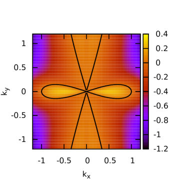
Figure 2: The $\lambda_{+}(k_{x},k_{y})$ function at $A=1$, $D=1$ and $\beta=-1$. The function is positive within the region marked by the contour line $\lambda_{+}(k_{x},k_{y})=0$.

This results in a length scale selection corresponding to the fastest growing periodic perturbation $\vec{k}_{\rm max}$ defined by the condition

$$\left.\frac{d\lambda_{+}(\vec{k})}{d\vec{k}}\right|_{\vec{k}_{\rm max}}=0$$ (102)

Figure 3: The $\lambda_{+}(k_{x},0)$ function at $A=1$, $D=1$ and $\beta=-1$.

For negative $\beta$, the $\lambda_{+}(k_{x},k_{y})$ function has two equal maxima along the $x$ axis located at

$$k_{x}^{2}=-2\beta\frac{-1+\sqrt{1+\frac{(A-D)^{2}}{4AD}}}{(A-D)^{2}}$$

It should be stressed that according to Eq. (93) the actual wave vector of the fastest growing perturbation is $\sqrt{\rho_{0}}\vec{k}_{\rm max}$. So, in agreement with the principle of similitude observed experimentally the characteristic pattern wavelength scales with the dislocation spacing $1/\sqrt{\rho_{0}}$. It is important to note at this point that the diffusion-like $\tau_{d}$ term introduced here plays a crucial role in characteristic wavelength selection. At $A=0$ (corresponding to $\tau_{d}=0$, see Eq. (36)) perturbations of all wave vectors would grow and there would be no mode of maximum growth rate. In accordance with this, by analyzing the stability of the homogeneous solution of the 3D continuum theory of dislocations proposed by Hochrainer et. al Hochrainer et al. (2007, 2014); Hochrainer (2015), Sandfeld and Zaiser concluded Sandfeld and Zaiser (2015) that the mean field and the flow stresses generate instability but they do not result in length scale selection.

Within the general framework introduced in the second section there is another way leading to dislocation pattern formation which can operate even if $A=0$, but which requires the consideration of higher-order gradients in the dislocation densities. Until now we have neglected the term proportional to $\partial_{xx}\rho/\rho^{3/2}$ in the expression for the flow stress in Eq. (34). Without going into the details of the derivation one can find that with this term, but with $A=0$, the evolution equations (83,V) get the form

$$\partial_{t}\delta\rho=-M_{0}b\partial_{x}\left[\tau_{0}\delta\kappa\right]$$ (103)

$$\partial_{t}\delta\kappa=-M_{0}b\Theta_{f}\partial_{x}\left[\rho_{0}\partial_{x}\partial_{y}\delta\chi-GbD\partial_{x}\delta\kappa\right]$$ (104)

$$-M_{0}b\Theta_{f}\left[\tau^{*}-\alpha\mu b\frac{\sqrt{\rho_{0}}}{2}\partial_{x}\delta\rho-\frac{Gb\eta}{\sqrt{\rho_{0}}}\partial_{xxx}\delta\rho\right],$$

where $\eta$ is a constant and for simplicity the terms related to $\tau_{a}$ are neglected. After substituting the solution given by Eq. (93) into Eqs. (103,104) in the flowing regime ($\Theta_{f}=1$) we get

$$\left(\begin{array}[]{cc}\lambda,&i(\dot{\gamma}^{\prime}+2\alpha^{\prime})k_{x}\\ ik_{x}[(\dot{\gamma}^{\prime}-\alpha^{\prime})+\eta k_{x}^{2}],&\lambda+Dk_{x}^{2}+T(\vec{k})\end{array}\right)\left(\begin{array}[]{cc}\delta\rho\\ \delta\kappa\end{array}\right)=0$$ (109)

Eq. (109) has nontrivial solutions if

$$\lambda(\lambda+Dk_{x}^{2}+T(\vec{k}))+k_{x}^{2}[(\dot{\gamma}^{\prime}+2\alpha^{\prime})(\dot{\gamma}^{\prime}-\alpha^{\prime}+\eta k_{x}^{2})]=0$$

leading to

$$\lambda_{1,2}=-\frac{Dk_{x}^{2}+T(\vec{k})}{2}$$ (112)

$$\pm\frac{\sqrt{[Dk_{x}^{2}+T(\vec{k})]^{2}-4k_{x}^{2}[(\dot{\gamma}^{\prime}+2\alpha^{\prime})(\dot{\gamma}^{\prime}-\alpha^{\prime}+\eta k_{x}^{2})]}}{2}$$

The condition to growing perturbation is

$$(\dot{\gamma}^{\prime}-\alpha^{\prime})+\eta k_{x}^{2}<0$$ (114)

Provided that $\eta>0$ and $\dot{\gamma}^{\prime}<\alpha^{\prime}$ there is again a region in the $\vec{k}$ space in which perturbations grow, and one can again find the wavelength corresponding to the fastest growing perturbation. It should be noted that in this case the length scale selection is caused by a second order effect in the sense that the term $\partial_{xx}\rho/\rho^{3/2}$ is obtained by the second order Taylor expansion in Eq. (17) while $\tau_{d}$ given by Eq. (36) corresponds to a first order one.

VI Conclusions

In summary the general framework explained in detail in section II and III is able to account for the emergence of growing fluctuations in dislocation density leading to pattern formation in single slip. The primary source of instability is the $\sqrt{\rho}$ type of dependence of the flow stress, but alone it cannot lead to length scale selection. As it is shown above there are two alternative ways (the diffusion-like term associated with the stress $\tau_{d}$, or the $\partial_{xx}$ type term in the flow stress) leading to characteristic length scale of the dislocation patten.

Irrespective of the pattern selection mechanism and in line with previous work Sandfeld and Zaiser (2015), we find that there are two requirements for patterning: First, the system must be in the plastically deforming phase, second, the rate of shear must not be too high ($\dot{\gamma}^{\prime}\leq\alpha^{\prime}$). This condition indicates that patterning as studied here can not be understood as a energy minimization process, despite the fact that the dynamics which we investigate minimizes an energy functional. This seemingly paradox statement becomes clearer if we consider the limit $\alpha\to 0$ where the mobility functions become trivial. In this limit, the critical strain rate where patterning vanishes goes to zero. Thus, the patterning is an effect of the non-trivial mobility function which introduces a strongly non-linear, dry-friction like behavior into the system. This aspect of the problem, which contradicts the low energy paradigm and emphasizes the dynamic nature of the patterning process, clearly should be further studied by extending the analysis into the non-linear regime.

In the limit of low strain rates, $\dot{\gamma}\ll\rho bM_{0}\tau_{\rm ext}$, the selected pattern wavelength becomes independent on strain rate. The predictions in this regime agree well with experimental observations: With $A=1.25$ Valdenaire (2015), $D=0.25$ Groma et al. (2006), $\alpha=0.2$, and $\nu=0.3$, we find a preferred wave-vector $|k_{x}|=\approx 0.42\sqrt{\rho}$ corresponding to a wavelength of about 15 dislocation spacings, in good agreement with typical observations. The preferred patterns corresponds to dislocation walls perpendicular to the active slip plane, again in agreement with observations and discrete simulations. This agreement does not mean that the present, very simple considerations alone provide a complete theory of dislocation patterning – in particular the essential aspect of dislocation multiplication, and hence work hardening, is missing. However, it indicates that we may capture some of the essential features of the real process.