Transient effects in Herschel/PACS spectroscopy

Abstract

Context. The Ge:Ga detectors used in the PACS spectrograph onboard the Herschel space telescope react to changes of the incident flux with a certain delay. This generates transient effects on the resulting signal which can be important and last for up to an hour.

Aims. The paper presents a study of the effects of transients on the detected signal and proposes methods to mitigate them especially in the case of the “unchopped” mode.

Methods. Since transients can arise from a variety of causes, we classified them in three main categories: transients caused by sudden variations of the continuum due to the observational mode used; transients caused by cosmic ray impacts on the detectors; transients caused by a continuous smooth variation of the continuum during a wavelength scan. We propose a method to disentangle these effects and treat them separately. In particular, we show that a linear combination of three exponential functions is needed to fit the response variation of the detectors during a transient. An algorithm to detect, fit, and correct transient effects is presented.

Results. The solution proposed to correct the signal for the effects of transients substantially improves the quality of the final reduction with respect to the standard methods used for archival reduction in the cases where transient effects are most pronounced.

Conclusions. The programs developed to implement the corrections are offered through two new interactive data reduction pipelines in the latest releases of the Herschel Interactive Processing Environment.

1 Introduction

The Herschel space observatory (Pilbratt et al., 2010) completed its mission on April 29, 2013 after performing a total of 23,400 hours of scientific observations during almost 4 years of activity ( 1446 operational days). One of the most used instruments aboard Herschel was the PACS spectrometer (Poglitsch et al., 2010). Approximately one quarter of the total scientific time was devoted to PACS spectroscopy. Although most of the observations were performed in the standard “chop-nod” mode, a substantial fraction (30% of the observations, corresponding to the 25% of the total spectroscopy time) used two alternative modes. The “wavelength switching” mode was released to users after the start of the mission to allow PACS spectrometer observations to be made in crowded fields where chopping was not possible. A year later, this mode was replaced by the so-called “unchopped” mode. By the end of the Herschel operation mission, this mode was used for approximately one-third of all PACS spectroscopic observations. The primary focus of this paper is to describe an optimal way to reduce data taken in the “unchopped” mode.

The PACS spectrometer was able to observe spectroscopically between 60 $\mu$m and 210 $\mu$m using Ge:Ga photo-conductor arrays. This type of detectors suffers from systematic memory effects of the response which can bias the photometry of sources and increase the noise in the signal. Such effects have been documented and studied for similar detectors on previous space observatories such as ISOCAM (Coulais & Abergel, 2000; Lari et al., 2001) and MIPS (Fadda et al., 2006, Fig. 17).

In this paper we briefly review the observational modes of the PACS spectrograph and the data reduction techniques. We describe how the “unchopped” mode is particularly sensitive to sudden changes in incident flux, and cosmic ray glitches, which cause memory effects in the detector responses. Finally, we introduce the technique used to correct most of these effects, and show a few selected examples. The methods and software described in the paper are now implemented in the Herschel Interactive Processing Environment (HIPE) (Ott, 2010). The comparisons presented in the paper are between the archived SPG (standard product generation) products, generated with HIPE 14.0 and calibration data version 72, and our pipeline in HIPE 15.

2 The PACS spectrometer

We recommend reading Poglitsch et al. (2010) and the PACS observational manual for a detailed description of the PACS spectrometer. As a way to introduce some terminology used in the paper, we give here a concise description of the instrument and how it works.

The PACS spectrometer was an IFU (integral field unit) composed by a matrix of $5\times 5$ spatial pixels (spaxels or space modules) covering a field of $47^{\prime}\times 47^{\prime}$ square arcminutes. The $5\times 5$ pixel image passed into an image slicer, which rearranged the $5\times 5$ two-dimensional image into one-dimension ($1\times 25$), which then fed a Littrow-mounted diffraction grating where it operated at $1^{st}$, $2^{nd}$, and $3^{rd}$ order. The first order (red) and second or third order (blue) were separated with a dichroic beam-splitter, where the spectra were re-imaged onto separate detectors. The wavelength range covered is 51-105 $\mu$m for the blue (choice of 51-73 and 71-105 $\mu$m for the $3^{rd}$ and $2^{nd}$ order) and 102-220 $\mu$m for the red, respectively.

The dispersed light was detected by two (low and high-stressed) Ge:Ga photo-conductors arrays with $25\times 16$ pixels. In the following we call spectral pixels the individual pixels of the two arrays. We call “module” or “spaxel” (from spatial pixel) the set of 16 spectral pixels corresponding to the dispersed light from a single patch of $9.4\times 9.4$ square arcseconds on the sky.

Since the instantaneous wavelength range covered by 16 spectral pixels is small ($\sim$1500 km/s for many observations), the grating was typically stepped through a range of grating angles during an observation. This operation is referred as a “wavelength scan”. During a standard observation, the desired wavelength range is covered by moving the grating back and forth. These movements are called up- and down-scans, since the wavelength seen by a single spectral pixel first increases and then decreases as the grating executes a scan first in one direction, and then back.

The other mobile part of the system is the chopper which lies at the entrance to the whole PACS instrument. This is a mirror which allows the IFU to point at different parts of the sky. In standard chop-nod mode, the chopping mirror is used to alternatively point rapidly to the source and then a background position, while maintaining the same telescope pointing. The largest chopper throw available is 6 arcminutes, which is a limitation of the chop-nod mode. If the chopper mirror is moved to larger angles, it can access two internal calibrators (BB1 and BB2) which are used for calibration during the slew to the target source.

Since the mirror is passively cooled, the emission of the telescope is significant, and typically dominates the total signal. For instance, in the red, the emission seen by a given pixel at 120 $\mu$m is around 300 Jy. This high telescope background level, although not generally desirable in IR astronomy, has the advantage that it helps to mitigate transient effects in the detectors by helping to keep the signal level constant at the detectors. A second property of the dominant telescope signal is that it is always present, and can be used as a relatively constant reference flux. This property can be positively exploited in the analysis of these PACS data.

3 Observational modes

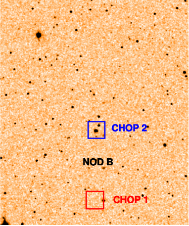
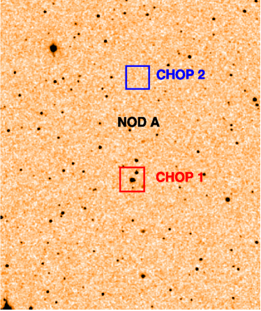
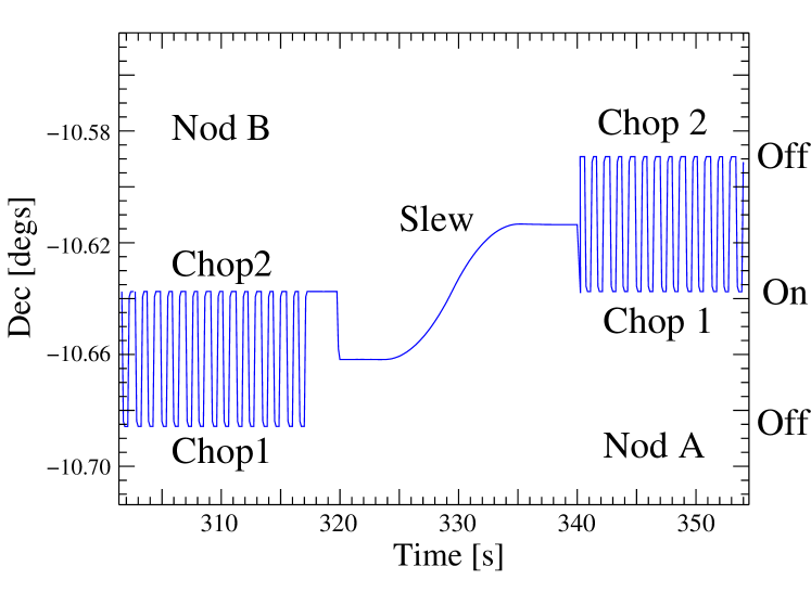
Figure 1: Example of chop-nod observation footprints (top), and observed position projected on the sky (bottom). In the first nod, the detector alternates between two optical paths to observe the object and the background. These paths have slightly different telescope background signals. In the second nod, the optical paths are inverted after slewing the telescope. By adding the two object-background differences, it is possible to remove the effects of the different telescope background levels.

Spectroscopic observations consist of a calibration block followed by a series of science blocks. The calibration block is performed when the telescope is slewing to reach the target and involves rapid chopping between the two internal reference black-bodies. The science target is then observed in one or more bands using either the “chop-nod” or the “unchopped” observational mode. The “chop-nod” mode is used for isolated sources and involves the continuous chopping between target and an “off” position. The “unchopped mode” is used to observe crowded fields or extended sources. It consists of a staring observation of the science target followed by an observation of the reference “off” position by moving the telescope. This mode replaced the “wavelength-switching” mode used for earlier observations. Instead of chopping, the “wavelength switching” used a wavelength modulation to move the line on the detector array by a wavelength equivalent to the FWHM of the line. This allowed the differential spectrum to be measured, but it was found to be inefficient during the verification phase and deprecated. Observations in “unchopped mode” suffered from detector transient effects. This paper is directed at ways of solving some of these problems within the HIPE software.

3.1 Chop-nod mode

The standard way to observe with the PACS spectrometer was the “chop-nod” mode. During a wavelength scan, the chopper modulates between an “on-source” and “off-source” position. In this way, any variation of the response slower than the chopping time can be subtracted using the “off-source” constant reference. However, since the on- and off-source chop signals follow different optical paths through the telescope, the observed telescope background emission is slightly different in the two chop positions. To remove this effect, the telescope is nodded. In the left panel of Figure 1 we show the first nod position (nod B) when the source is observed in the chop 2 position. The right-hand panel shows the situation after a small slew which places the source in chop position 1 where the observation is repeated (nod A). The optical paths used to observe source and off-field are inverted so that the average of the “source minus off” signals is largely unaffected by the different telescope backgrounds.

Two types of submodes are defined in the chop-nod mode. In the case the observation involves an unresolved line, the “line chop-nod” mode defines an optimal way to observe the line and the surrounding continuum. If a larger wavelength range is required, the “range chop-nod” mode can be used to manually enter the range of wavelengths to be scanned by the grating.

The data reduction is done on each individual pixel. The simplest reduction technique uses the calibration block to compute the average response during the observation. The response is defined for each pixel as the ratio between the measured and expected signal from the internal calibrators which was measured in the laboratory. The measured signal is composed of the telescope background ($T_{A}$ and $T_{B}$ in the two chopping positions), source flux ($s$), and dark ($d$) signal. The telescope background is dominated by the emission of the primary mirror, and depends on the temperature of the spot which is seen by the detector. Because of differential variations in the mirror temperature, and its emissivity with position on the mirror, the different chopper positions tend to see differing degrees of telescope background. Although, during a given observation, the overall temperature of the mirror changed slowly, it was measured to vary due to changes in illumination of the spacecraft by the Sun on longer timescales than a single observation.

For the measured signal $C$, in $V/s$, in a chop-nod observation we have:

$$\begin{array}[]{c@{\:=\:}r@{\quad}c@{\:=\:}r}C_{1}\hfil\>=\>&(T_{A}+d+s)\cdot R(t)&C_{2}\hfil\>=\>&(T_{B}+d)\cdot R(t)\\[8.61108pt] C^{\prime}_{1}\hfil\>=\>&(T_{A}+d)\cdot R(t)&C^{\prime}_{2}\hfil\>=\>&(T_{B}+d+s)\cdot R(t)\end{array}$$ (1)

for the two chop positions in the first ($C_{1}$ and $C_{2}$) and second nods ($C^{\prime}_{1}$ and $C^{\prime}_{2}$), respectively. Here $R(t)=\rho_{\lambda}\cdot r(t)$ is the product of the relative spectral response function (RSRF) $\rho_{\lambda}$ and the response function $r(t)$ (V s^-1 Jy^-1) which can vary with time. T_A and T_B correspond to the signal detected from the telescope background at the chopper positions A and B, respectively.

The simplest technique consists in estimating the signal source by computing the differential signal, $\hat{s}$, between the chopping positions and combining the nods:

$$\hat{s}=[(C_{1}-C_{2})+(C^{\prime}_{1}-C^{\prime}_{2})]/(2\cdot\rho_{\lambda}\cdot r_{CB}),\leavevmode\nobreak\ \leavevmode\nobreak\ \leavevmode\nobreak\ \leavevmode\nobreak\ \leavevmode\nobreak\ \leavevmode\nobreak\ \leavevmode\nobreak\ [Jy]$$ (2)

where $r_{CB}=\left<r(t)\right>$ is the average response estimated from the calibration block. As we can see, the method works if $r(t)$ is approximately constant during a chopping period (1 sec) so that the subtraction cancels the effect of a transient. This approach was used by the so called SPG (standard product generation) pipeline to populate the Herschel Science Archive (HSA) for chop-nod observations until recently.

Since SPG 13, an alternative approach exploiting the knowledge of the telescope background is used. This technique does not require the application of the RSRF and response corrections since it uses the ratios between the observations in the two chopping directions. Nevertheless, the accuracy of the results depends on the knowledge of the mean telescope background. Also, ratios introduce more noise in the final signal with respect to the standard reduction.

In formulae, if we define normalization as:

$$N=\frac{C_{1}-C_{2}}{C_{1}+C_{2}}+\frac{C^{\prime}_{1}-C^{\prime}_{2}}{C^{\prime}_{1}+C^{\prime}_{2}}=\frac{2s}{T_{A}+T_{B}+2d+s},$$ (3)

the signal normalized to the average telescope background can be expressed as:

$$\frac{s}{\left<T\right>+d}=\frac{s}{(T_{A}+T_{B})/2+d}=\frac{N}{1-N/2}.$$ (4)

The source flux can be therefore derived by multiplying the normalized signal by the telescope background (dark included). This method frees the result from the effects of the variable response although it requires the knowledge of the dark. Since PACS has no shutter, the dark was measured in the laboratory before the launch of Herschel. It is not known with great accuracy although its value is negligible with respect to the telescope background. The telescope background was derived in flight by calibrating the emission of the mirror with observed spectra of bright asteroids.

3.2 Unchopped mode

At the end of the verification phase, the “wavelength switching” mode (see Poglitsch et al., 2010) was released and used in a few key programs. Several disadvantages became apparent with this mode during its early use, leading to its replacement with the “unchopped” mode. For example, by construction, the continuum of the source could not be measured. Moreover, only observations of unresolved lines could be measured correctly. Asymmetric lines or lines broader than the wavelength switching interval were found to be difficult to recover. For large wavelength ranges, SED shape variations can lead to peculiar baselines in the final differential spectrum. This made observations over large wavelength ranges challenging. Finally, the rapid switching of the grating between two distant wavelength positions created mechanical oscillations which required a long time to damp. This effect was more severe in space than during ground testing, leading to longer time intervals between useful observational samples and thus preventing an efficient removal of rapid response variations.

It appeared clear that performing a slow grating scan while staring at an object, followed by a similar observation pointed to an “off” position, yielded superior results compared with “wavelength-switching”. This “unchopped” mode had the advantage of allowing large wavelength range scans, such as far-IR SEDs of confused or extended regions. Unlike the “chop-nod” mode, where the two chopper positions sample different optical paths and therefore different mirror temperatures, in the “unchopped” mode the optical paths used for on- and off-source observations are the same. Therefore, the mirror temperature in the on- and off-source are exactly the same. Moreover, in the case of chop-nod, the footprint of the detector on the sky rotates slightly between the two chop positions (see the PACS observer manual, Figure 4.7). The effect, though small, is worse for the larger chopper throws. This means that in the two nod positions, the only spaxel seeing precisely the same part of the source is the central one. Spaxels further from the center become successively mismatched in the two nods. So, the reduction works best for the central spaxel. This problem does not exist for the “unchopped” mode because the observation of the on- and off-positions are made with a fixed central chopper position.

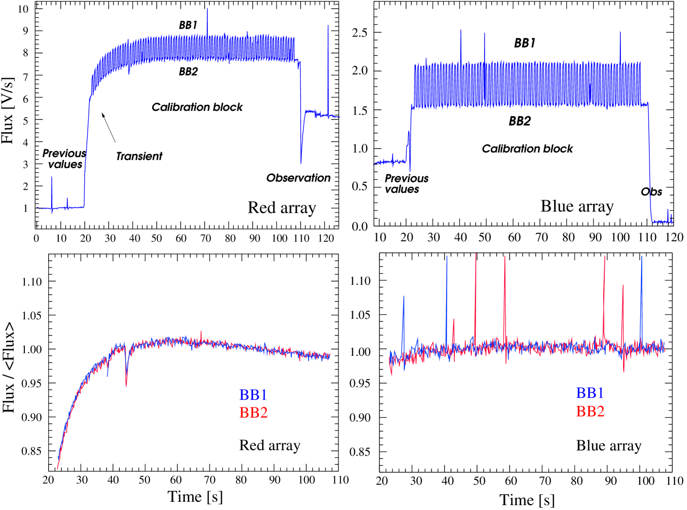
Figure 2: Transients affecting the calibration block for the red (left) and blue (right) arrays. During the calibration block, the detectors see alternatively the two blackbodies (top panels). Since the initial flux is significantly different from the fluxes of the internal blackbodies, a strong transient occurs during the first minute of the observation. The signals normalized to the median values of each blackbody (bottom panels) show how the same transient affects the fluxes from the two blackbodies (blue and red lines). The transient effect is more pronounced for the red array.

The “unchopped” line and range modes were released on September 2010, superseding the previous “wavelength switching” mode. A specific “unchopped” mode for bright lines was released on April 2011.

In “unchopped” mode, a complete wavelength scan is done first on the “on-source” (hereafter ON) position and then later on a “off-source” (hereafter OFF) position clear of source emission. Unfortunately, variations of the response during the ON scan cannot be corrected using the OFF scan because the two scans are performed at different times. So, although unchopped observations offer some advantages over the chop-nod mode, the effects of transients require mitigation. In this paper, we show the typical transients found in the signal, and some techniques to model and subtract them.

Three different sub-modes exist for the unchopped mode:

• unchopped line, for single line observations.

• unchopped bright line, for single bright lines. It is 30% more time efficient than the standard line mode since bright lines require less continuum to compute the line intensity.

• unchopped range, for observations of the continuum or a complex of lines.

A further difference between these sub-modes is that the reference OFF is observed during the same AOR (Astronomical Observation Request) in the case of the “unchopped line”, but has to be provided as a separate AOR in the “unchopped range”. In order to ensure the observations are performed sequentially, the OFF observation in the unchopped range scan is concatenated to the main observation within the observation sequence.

4 Transients

The term “transient” refers to a delayed response of a detector to the variation of the incident flux. Transients are particularly evident after sudden variations of flux on detector arrays (see, e.g., Coulais & Abergel, 2000). In Figure 2 we show the signal detected during the calibration block when the chopper points alternatively between the two internal black bodies (which have different temperatures). Passing from the previous observation to the internal black bodies causes a clear transient effect which is more important in the case of the red array (left panels). When the signal is normalized to the asymptotic flux (bottom panels), the response variation becomes evident. It is interesting to note (left bottom panel) that the short transients due to cosmic hits on the array have a timescale longer than the chopping time. This allows the correction of these effects using the “chop-node” mode.

We can classify three separate types of transients:

• continuum–jump transients: transients due to a sudden change of the incident flux from one almost constant level to another almost constant level;

• cosmic ray transients: transients induced by cosmic ray hits which produce glitches, followed by a response variation;

• scan dependent transients: transients along a wavelength scan produced by rapid variations of the (dominant) telescope background and continuum (in the case of a bright target).

It is worth mentioning that the Standard Product Generation (SPG) pipeline, which populates the HSA, does not use any type of transient correction. So the products available in the archive for the “frequency switched” and “unchopped-mode” observations contain many transient effects that could adversely affect science goals. However, from HIPE 14 onward, users have the option of processing their data with special scripts designed specifically to correct transients. The current paper describes how these corrections are made. In the following we describe in detail the different types of transients.

4.1 Continuum-jump transients

A sudden change in the illumination of a detector pixel passing from one flux level to another, can induce a major transient in the signal. This occurs typically at the beginning of each observation just after the completion of the calibration block. Because of the difference between the flux from internal calibrators and the telescope background, a transient is usually visible during the entire observation.

Another common form of this kind of transients is when a change of band, or change of wavelength occurs while observing a source. For example, the user may have requested two different lines occurring at different wavelengths. When the grating is commanded to access a different part of the spectrum, or change to a completely different region of the spectrum, a jump in the signal usually occurs because of the changing emission spectrum of the telescope background at different wavelengths (see Section 5.2). If the source is very bright, differences in continuum level from the source can also induce a transient.

If the source continuum is negligible with respect to the telescope background, it is possible to normalize the signal during the whole observation to the telescope background which has been previously calibrated. The transient due to the jump in continuum between the calibration block and the target observation appears clearly, see Figure 3. It is possible, in this case, to fit the behaviour with a model and subtract it from the observation. It is interesting to note that, without this correction, an OFF observation can have a measured flux greater than an ON observation if it happens to be performed during a period of response stabilization. This effect is not taken into account by the SPG pipeline, so that many observations in the archive have an artificial and confusing negative background.

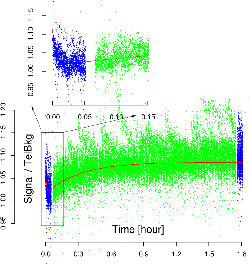
Figure 3: When the signals from a spaxel are normalized to the expected telescope background a long-term transient after the calibration block becomes clear. In this example (an observation of M81, ObsID 1342269535) an OFF position is observed at the beginning and at the end of the observation (blue dots), while a 2x2 raster observation is performed in the middle (green dots). Since the continuum emission of the object is negligible with respect to the telescope background, it is possible to fit the general long-term transient (red line) and correct the signal. Note that many huge transients appear in individual spectral pixels because of cosmic ray hits on the detectors. If this correction is not made, and an average background is subtracted from the signal, the final image will present an artificial gradient and the flux will be negative in some regions. Top inset panel: a close-up of the initial part of the signal just after the calibration block, showing the strong transient. The periodic variation in the signal is a left-over from the imperfect telescope background estimate used for normalization. The empty spaces between points occur during telescope slewing.

Some observations that used the unchopped mode contained requests for more than one band in a single AOR. For extended sources, a typical raster observation allows one to cover an extended region by moving the telescope to cover a grid of positions. However, for efficiency reasons, the AOR was designed to cycle through all the requested bands at each raster position, before moving the telescope to the next position in the raster sequence. An unexpected side effect of this strategy was the generation of transients at each band change. It is not possible to remove these jump–transients in a clean way in case of such multiple-band observations.

There is an important lesson to be learned from this experience with PACS. In retrospect, it would have been better to observe the complete raster in a single band, before cycling to the next band. This would have minimized the effects of band-induced jump-transient. We advise that any future mission where transient could be an issue, should avoid as much as possible sudden changes in flux during the observation. This is probably the case of FIFI-LS onboard SOFIA, which is essentially a clone of the PACS spectrograph. Unfortunately, when the observational mode was introduced for Herschel, the reduction pipeline was not fully developed, and it was very difficult to evaluate all the effects. Since the response was known to stabilize relatively fast, it was assumed that the effect of a band change was minimal, compared with the advantage of being more time efficient. Experience later showed that jump-transient transient caused by band changes appear to limit the quality of the observation, even with the most advanced data reduction. Indeed, we are able to see jump-transients even in the blue channel, which has the fastest response stabilization compared with the red (see Figure 4).

4.2 Cosmic ray transients

It is well known that for Ge:Ga detectors, energetic cosmic rays usually produce glitches in the signal, followed by response variations. Depending on the energy of the cosmic ray, the glitch can be followed by a tail or the variation can be more complicated (lowering temporarily the response). A similar behavior was noted in the past for pixels in the ISOCAM array on the Infrared Space Observatory (see, for example, Lari et al., 2001). We will show that the response variation can be described with a combination of exponential functions (see Section 5). The main challenge to correcting and masking the damage in the signal from cosmic ray hits is to select the most significant events, and then find the starting time which marks the beginning of the discontinuity in the signal.

4.3 Scan dependent transients

Finally, in the case of observations spanning an extended wavelength range, rapid variation of the continuum during the wavelength scan produced transients in the signal (see Section 5.4 for an example). In some observations, this last effect is responsible for different apparent fluxes in the source spectrum for upward and downward scans over the same wavelength range. Luckily, many PACS observations using the unchopped mode targeted only one line with a short range scan. For these cases, scan-dependent transients had negligible effects. It was found to be important only for observations which scanned over extended wavelength ranges. As a result, two different interactive pipeline scripts (accessible within HIPE as so–called ipipe scripts) have been written to treat the “unchopped line” and “unchopped range” cases separately.

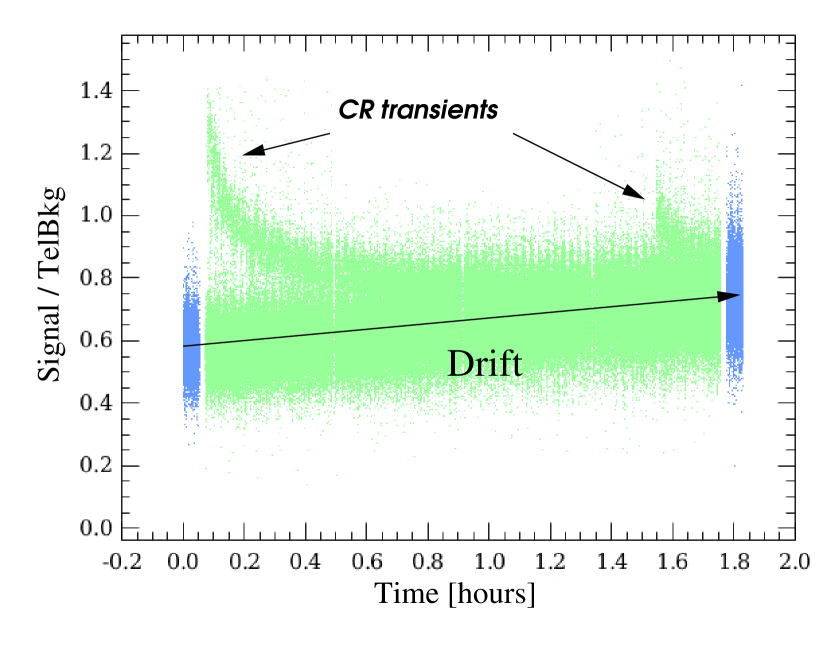
Figure 4: Long-term transient for the pixels of module 16 in the blue channel of the obsid 1342246963. One of the pixels shows also a transient due to a cosmic ray hit. There is a 30% variation between the two ends of the observation. Blue and green dots refer to off-target and on-target parts of the observation, respectively.

5 Detecting and modeling transients

To detect, model, and correct transients in the signal, one has to decouple the signal and the effect of the transients. The best way to proceed is to obtain an estimate of the response by normalizing the signal to the expected spectrum. As we will see in the following sections, if the source emission is negligible with respect to the telescope background, the ideal way to proceed is to normalize the signal to the expected telescope background. If the source emission is not negligible, one has to have a better guess of the signal. One possibility is to assume that the detector eventually stabilizes after a jump in the continuum, so that one can use the last scans near the end of the observing sequence to estimate the “true” continuum level. This asymptotic level can then be used to normalize the entire signal to reveal the jump–transient. Once the transient is revealed in this manner, it can be fitted and removed from the signal.

Once the transients due to expected continuum-jumps are corrected, it is possible to obtain a first estimate of the final spectrum, combining all data from all independent up and down scans, and measurements made with all 16 pixels combined together. Once this average spectrum is created, it can be used to revisit the individual pixel responses by normalizing their signal to this “first guess” spectrum. In this way, each individual detector pixel response to can be studied for the effects of cosmic ray transients, and these CR transients can be either corrected or masked. In the following, we describe the model used to fit the response as a function of time and the algorithms applied to the signal to mitigate the effect of the transients.

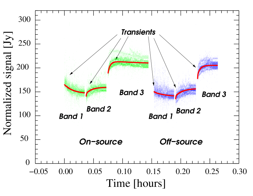
Figure 5: The central spaxel of an observation of NGC6543 (ObsID 1342215704) with three lines observed. For each observation block, the signal in each wavelength scan is divided by the last scan and normalized to its asymptotic median flux. The red line shows the transient model fitted. The first block comes after the calibration block (not shown) whose flux is higher than the continuum during this part of the observation. The three lines are observed first on the target (green dots) and then on the OFF position (blue dots). The gaps in these science data correspond to the time spent moving the grating, and slewing to the OFF position. Also in this case some pixels appear to behave differently because of the impact of cosmic rays.

5.1 Model

The response variations can be described in general using a combination of exponential functions. We found that a combination of three exponential functions closely describe the several different cases of transients observed.

$$f(t)=a+a_{short}e^{-t/\tau_{short}}+a_{medium}e^{-t/\tau_{medium}}+a_{long}e^{-t/\tau_{long}}$$ (5)

The parameter $a$ corresponds to the median level of the normalized signal. In the case that the response is obtained by normalizing the signal to the last scans, $a$ is fixed to unity by construction. The three exponential functions have very different timescales. A first function accounts for the fast variation of the signal just after the flux change or a cosmic hit. The timescale is between 1 and 10 seconds. The second term has an intermediate timescale (between 10 and 80 seconds). Finally, the third term accounts for the long-term variation of the signal and has the longest timescale (between 200 and 1200 seconds). In the case of cosmic ray induced transients, the $a_{short}$ coefficient is always positive, whereas for the continuum-jump transients $a_{short}$ can be either positive or negative depending on the direction of the jump. The parameter space considered for the fitting in the two cases is similar.

In the case of cosmic rays, the time constant $\tau_{short}$ is kept lower than one second. For the continuum-jump transient, the parameter space for $\tau_{short}$ considered is between 1 and 10 seconds. For the other two time constants, the parameter boundaries are $10<\tau_{medium}<80$ seconds and $\tau_{long}>100$ seconds.

5.2 Correcting continuum-jump transients

If the continuum of the source is negligible with respect to the telescope background, it is possible to see the long-term transient caused by the calibration block all along the observation by normalizing the signal to the expected telescope background (see Figure 3). If this effect is not corrected and an average background is subtracted from the signal, there will be parts of the image with a signal lower than the average background which will have negative fluxes at the end of the data reduction. Even worse, in mapping observations, each raster position taken at a different phase of the transient will have a different continuum level resulting in an artificial gradient in the final image (see later in Figure 15).

Unfortunately, this correction depends on the knowledge of the telescope background emission. The current model available through HIPE is fairly accurate for the red array, while the situation is slightly worse for the blue array.

There are several situations where the simple correction above will not work. In the case of a very bright continuum, the normalization of the signal by the telescope background will not be appropriate, and this will make any correction difficult. Another case is that of a multi-band observation taken consecutively. In Figure 5 we show an example of an observation taken in 3 different bands. At the beginning of each observational block (observation of one band) there is a clear transient introduced by the sudden variation of the continuum level.

To correct the transients in both of these cases, we can normalize the signal to the flux detected during the last wavelength scan of each observational block. We make the assumption that the detector response has stabilized by this time. This assumption works well in the case of long observations ($\sim$1 hr). In the case of shorter observations, a little bias will remain in the data since the asymptotic level has not yet been reached.

5.3 Correcting transients caused by cosmic rays

The most disruptive transients are caused by the impact of cosmic rays on the detectors. Since they happen at random times with different energies, they cause unpredictable changes in the baseline of the data which can last from several minutes up to one hour. The main difficulty in fitting these transients with our model is to disentangle the real signal from the variation in response caused by the cosmic ray impact, and to detect the time when the impact occurs. Cosmic ray events are so frequent that, in practice, we must set a threshold above which we attempt to correct the signal.

Lebouteiller et al. (2012) developed a procedure to identify features associated with transients using a non-parametric method (multi-resolution transform of the signal and identification of patterns on a typical scale). The features found were then fitted with an exponential, and subtracted from the signal. This algorithm is identical to the one developed for the treatment of ISOCAM data (Starck et al., 1999).

The approach we described in our paper is different in both the way we identify the cosmic ray events, and how remove them. Our methods are similar to those developed by Lari et al. (2001) for the treatment of ISOCAM data, although the algorithms presented here differs in several significant details. First we obtain an approximation to the final spectrum cladding all the individual pixels that contribute to the scan (the “Guess” spectrum). Next, the signal for each individual pixel is normalized by this spectrum to obtain an estimate of the response. At this point, the discontinuities in the response are identified, and only the most significant are selected. We fit the model (equation 5) to the response in the interval between two consecutive discontinuities. A correction is then applied to the original signal to attempt to remove the effect of the cosmic rays. In the following, we describe in detail each one of these steps.

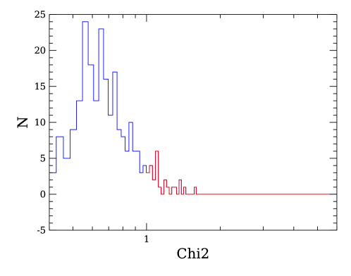
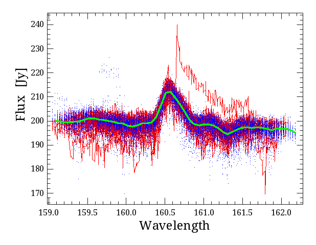
Figure 6: An example of how we estimate the “Guess” spectrum for the C+ line of Arp 220 (obsID 1342202119). We compute the histogram of the normalized $\chi^{2}$ of each individual spectral scan with respect to the median spectrum (top panel). The blue line shows the well behaved scans and the red line shows those to be rejected. The Guess spectrum (bottom panel; green line) is the result of co-adding the well behaved scans (blue lines). The scans with $\chi^{2}$ deviating more than 3$\sigma$ from the median value are discarded (red lines).

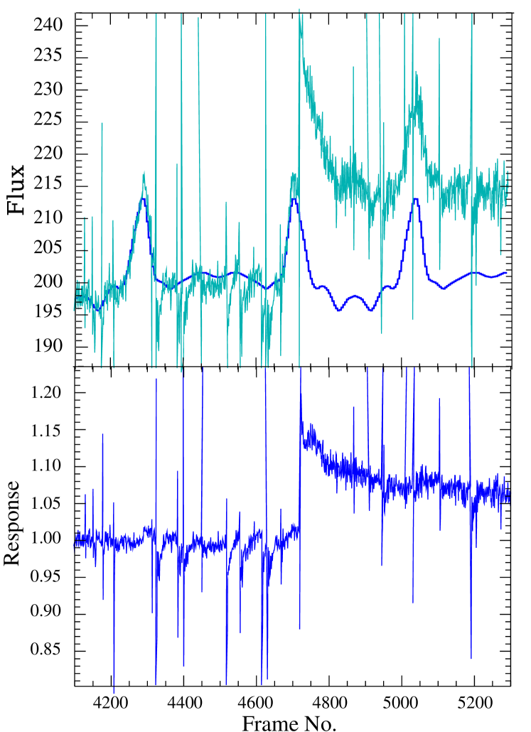
Figure 7: Top panel: A comparison of the observed signal of a single spectral pixel (cyan) with the “Guess” signal (blue; see text). The signal is plotted against the Frame Number, which is a function of time during the scan. We show three scans in the figure (two up and one down) which captures the C+ line shown in the previous figure. Just after the frame number 4720 a strong cosmic ray hits the detector producing a sudden change of the response of the detector. Bottom panel: The ratio of the two curves, i.e. the response of the pixel as a function of frame number. Many transients are clearly visible, in particular the huge transient after frame number 4720.

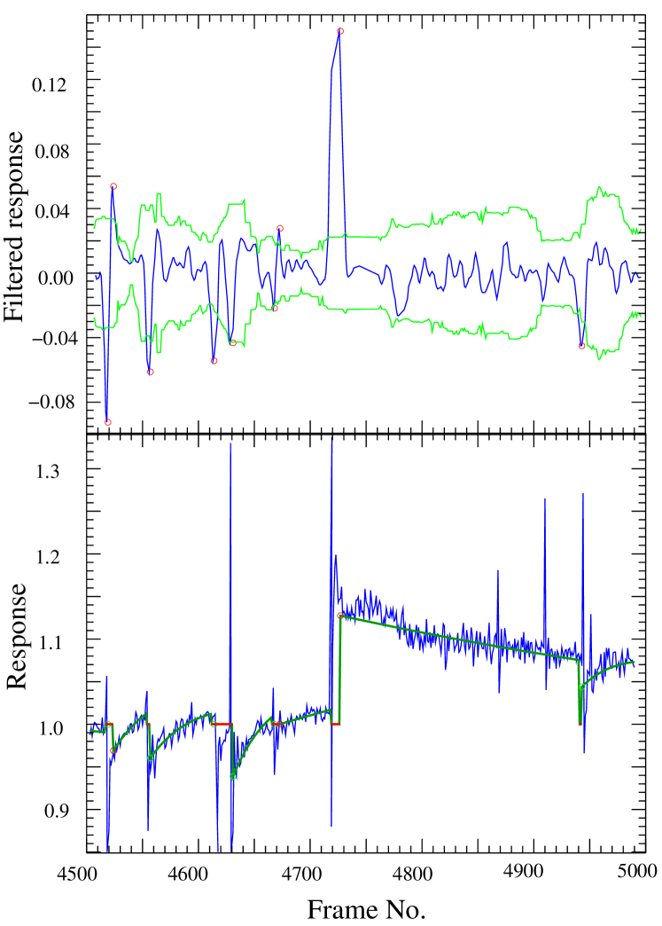
Figure 8: On the top panel, part of the response convolved with the first derivative of the Gaussian with dispersion equal to two frame units. This width gives the best sensitivity to sudden changes of the response caused by cosmic ray hits on the detectors. The green lines mark the region of $\pm 5$ times the local dispersion and the red circles marks the starting points of transients. In the bottom panel, the responsivity for the same block of frames with each interval between two consecutive discontinuities in the response fitted with our transient model (dark green). The red points mark the frame masked because the interval between two consecutive discontinuities is too short (less than 10 frames).

5.3.1 Estimating the “Guess” spectrum

We assume that the continuum jump transients have been corrected to this point. We need to identify the scans affected by severe transients, and discard them to obtain a good first guess of the spectrum. This step is particularly important in the case of low redundancy, since even a few bad scans can compromise the coadded spectrum. The procedure to obtain a guess spectrum is iterative. The first step consists of computing a median spectrum by coadding all the wavelength scans for the spectral pixels which contribute to a given spaxel. The spectrum is obtained by computing the median of all the valid fluxes for each bin of a wavelength grid: the median spectrum. Scans with very deviating values compared with the median spectrum are rejected. The scans with $\chi^{2}$ values which deviate more than 3$\sigma$ from the median of the $\chi^{2}$ distribution are discarded and a new median spectrum is computed (see top panel of Figure 6). To obtain a robust estimate of the dispersion of the distribution, we make use of the median absolute deviation (or MAD). The procedure is iterated three times to obtain a clean median spectrum which serves as “Guess” spectrum. Figure 6 shows visually how the process works in the case of an observation of the C+ line of Arp 220. The procedure works because of the high redundancy of the PACS data, which has a minimum of four up-and-down scans for each of the 16 spectral pixels.

5.3.2 Finding significant discontinuities

By normalizing the signal of each pixel by the expected flux of the Guess spectrum, we obtain an estimate of the response as a function of time for each pixel. This function can be used to study the effect of cosmic rays on the signal by selecting the most important ones, fitting the transients after them, and eventually masking part of the signal excessively damaged by the effect of cosmic ray impacts on the detector. In Figure 7 we show an example using the M82 C+ spectrum. Here the Guess signal is compared with the signal from a single pixel, allowing the discontinuities to be easily seen.

To correctly fit the transients, one has to identify the starting point, i.e. the moment at which the discontinuity in flux appears in the signal. This is a classical problem of signal theory and it has been shown (Canny, 1986) that the optimal filter to find discontinuities in a mono-dimensional signal is the first derivative of a Gaussian. The dispersion of the Gaussian was found empirically to be two frame units (equivalent to 0.25 s). If we convolve the response with this filter, spikes appear just after cosmic rays impact the detector. As shown in Figure 8, we can select the most important ones by comparing their intensity to the local noise in our response estimate. In our algorithm we make a cut of 5 $\sigma$ to select the significant events.

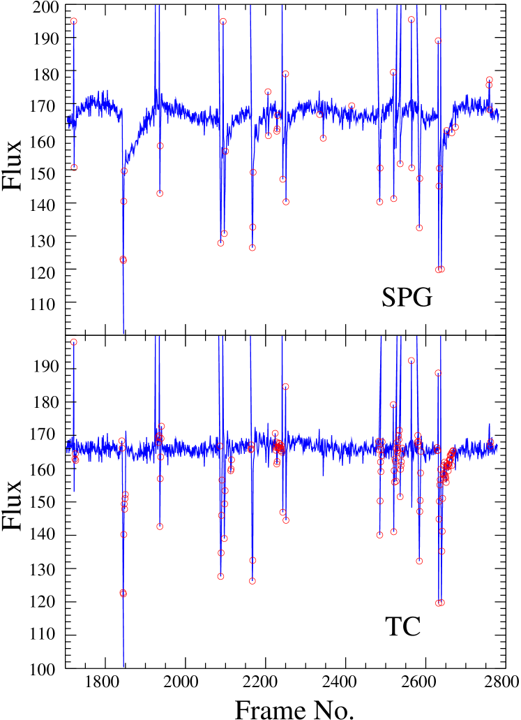
Figure 9: Comparison between masking in the SPG pipeline (top) and transient-correction pipeline (bottom). Signal is blue and masked frames are represented as red circles. The SPG pipeline masks a few deviant frames as GLITCHES, while the transient-correction pipeline masks frames either as GLITCHES or as UNCORRECTED. As a result, the signal from the SPG pipeline will contain unmasked residuals of big transients, while the transient-correction pipeline will either correct the transients or masked them completely. This leads to a big reduction of noise in the final reduction with respect to the product from the SPG pipeline.

5.3.3 Masking and computing the response

At this point we break the signal in intervals between two consecutive discontinuities, and fit the model (equation 5) in each one of these intervals. If the cosmic rays occur too close together (less than 10 frame units) we simply mask that part of the signal timeline. The resulting model response and masked regions are then applied to the original signal to remove the effect of the transients. This automatically corrects the signal for variations in the response after cosmic ray impacts, as well as correcting for large offsets in individual scans relative to the median signal.

One main difference with the reduction pipeline for chopped spectroscopy is that, at this point, there is no need for the application of a spectral flat field correction. In the standard pipeline, this is a separate task that takes into account small variations of the response in the different spectral pixels. Our modeling is able to automatically rescale all the pixels relative to the same spatial module in each observational block without any further operation.

The net effect of all our corrections is to significantly decrease the noise in the final coadded spectrum compared with the SPG pipeline. Although the SPG pipeline attempts to mask larger transients, important residuals remain (see Figure 9).

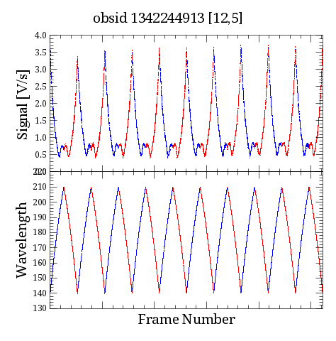
Figure 10: Signal variations as a function of the wavelength scan. To see the effect of the flux variations on the measured signal, we can compare the signal measured during the up-scans (blue parts) with the one measured during the down-scans (red parts).

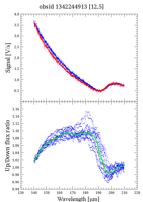
Figure 11: Top panel: flux in the up-scan (blue) compared to the flux in the down-scan (red). When the incident flux is decreasing (blue line between 140 and 195 $\mu m$) the measured flux is higher than that measured when the flux is increasing (red line in the same wavelength region). The situation is inverted between 195 and 205 $\mu m$, while the two fluxes are very similar in the wavelength region beyond 205 $\mu m$ where there is no big variation in flux. Bottom panel: ratio between up- and down-scan measured fluxes for all the 16 pixel in a space module. The behaviour is very similar.

5.4 Correcting scan dependent transients

For many of the PACS spectra, only a small wavelength range is observed. In this case we can consider that the continuum is essentially constant during the observation. So, during a wavelength scan there is almost no variation in the incident flux which could cause transient effects on the signal. This is not the case in observations of extended wavelength ranges, where the continuum can vary substantially during the scan. This leads to transient behaviour which becomes apparent when comparing the scans in two opposite directions. In Figure 10, we show that during up and down scans, the incident flux can change by, in this example, a factor of 7. This leads to a large transient.

In Figure 11 (top panel) the ratio of the two fluxes shows clearly the effect. Here we consider only one scan for a given spaxel. For the up-scan (blue points), we see the flux decreases as we scan to longer wavelengths. However, when we scan back with a down-scan, (red points) there is a systematically lower signal compared with the up scan. This is due to transient behavior caused by the rapidly changing flux during the scans. The effect is clearly shown in the ratio of the up and down scans (bottom panel of Figure 11). When the flux is changing very rapidly (between 145–190 $\mu$m), the up-scan flux is 10% higher than the down-scan flux. However, from 190–210 $\mu$m, where the flux change is much smaller (only a factor of two), the effect of the transient is also smaller (less than 2%).

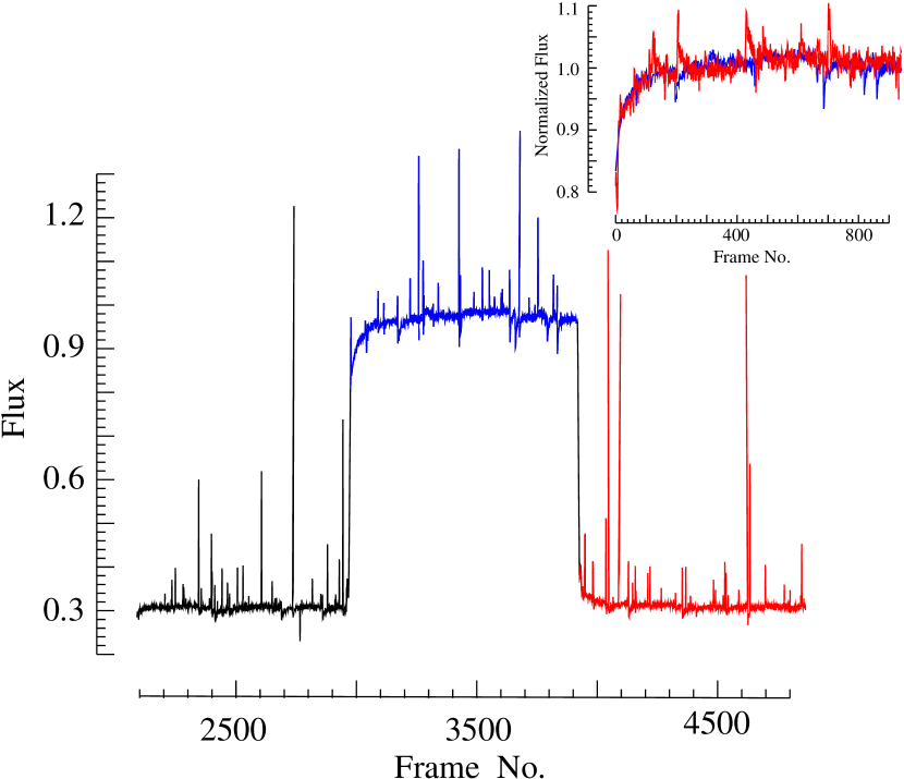
Figure 12: Transient effects on the measured signal when changing between two grating positions performed during an engineering observation during OD 27 (see text). In the inset, comparison of the upward (blue) and downward (red) transients. The downward transient has been flipped to compare the two behaviours. For a regime of flux changes similar to the one found in the range observations, the two transients follow essentially the same behaviour. This justifies the choice of getting the median signal between up- and down-scan signals.

Before we describe in detail how we apply a correction for this kind of transient, we first need to demonstrate that the transient caused by a sudden increase in continuum has a similar form to that of a sudden decrease in continuum. We will use this symmetrical behaviour of transients to provide a solution to the problem. To prove this symmetry, we consider an observation which was especially designed to induce transient behaviour of the detectors during observational day 27 (obsID 1342178054). In this observation, the grating was moved to several different positions to have different levels of flux on the detectors. After each move, the grating was halted for 4 minutes to allow stabilization. We show in Figure 12 a part of this observation to demonstrate the response to sudden jumps in recorded flux. The figure includes the signal readout just before (black line) a sudden change in the position of the grating, which then induces an upward transient and new stabilization (blue line). After a suitable interval, the grating is changed back to the original position leading to a downward jump and transition (red line), followed again by a period of stabilization. To investigate the shape of the upward and downward transients induced by this change in continuum, we show in the inset figure, the normalized signal for the upward– and downward–going signal, but with the downward signal flipped in sign to allow a close comparison. If we ignore the cosmic ray transients which are present, the behavior of the upward–going (blue) and downward–going (red) transient responses are almost identical.

In the above example, the largest part of the transient response occurs within a time interval of approximately one minute, and the example we chose corresponded to a change in flux of about a factor of three. We recall that in Figure 11, the up-and-down scan induced changes in continuum which were larger than this over the whole scan (which lasted two minutes), but are about the same order (roughly a factor of three) in one minute. Therefore, the test of the hypothesis that the symmetry in the shape of the upward and downward transient is valid.

If we make the assumption that indeed the upward– and downward–going transients have similar behaviors (except for the sign), this suggests a workable way to correct for the transients in a long scan over a rapidly changing continuum. Because of the symmetry, we can assume that the differences between the fluxes in Figure 11 is entirely due to transient behavior. This means that a reasonable solution is to scale the up- and down-scan values of the flux to the average of the two values at each wavelength interval. With this simple solution, according to the observation in Figure 12, the flux recovered is within a few percent of the asymptotic incident flux. We note that a change of a factor of three in the continuum in one minute (as in the above example) is an extreme case. In most observations, the changes in flux throughout a scan are likely to be much less.

6 Examples

In the following section we provide a few examples which show the improvements introduced by our transient-correction algorithms, as compared with the standard unchopped-mode HIPE analysis (SPG pipeline, vers. 14). We remind that it is important to avoid executing pipeline scripts blindly without examining the effects of the corrections in the different steps of the reduction process.

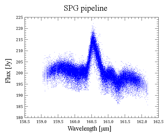
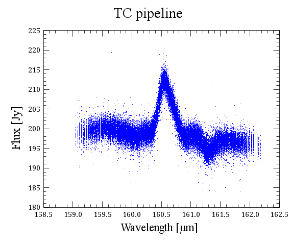
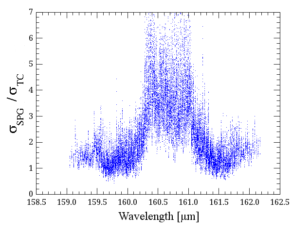
Figure 13: Top : SPG and transient-correction pipeline reductions of the central pixel of an observation of Arp 220 (obsID 1342202119). Bottom: ratio of standard deviations of the SPG and the transient-correction pipelines.

In this section we also show a few comparisons of observations made with unchopped and chop-nod mode of the same targets, to show how the reduction described in this paper gives consistent flux calibration for the same observed lines.

6.1 Line

As an example of the improvement in the reduction of a line unchopped observation, we show here an observation of Arp 220 (obsID 1342202119). We show in Figure 13 (top left panel) the cloud of flux–points for the central spaxel of the spectrometer array after passing the raw data through the SPG pipeline. In the top right panel of the same figure, the same observation was processed using the algorithms described in this paper. It is clear that the points are much less spread in the case of the transient–corrected data compared with the SPG pipeline. To evaluate the improvement in a more quantitative way, we computed for a given flux point, the dispersion in the surrounding 30 points, and then plot the ratio between the values for the two pipelines (bottom panel). The SPG pipeline has a standard deviation 40% larger in the continuum surrounding the line, as compared with the transient-corrected data. On the C+ line itself, the standard deviation is $3\times$ larger for the same comparison. We note that the faint absorption feature at 161.3 $\mu$m is much better defined in the reduction with transient corrections. The noise of the SPG pipeline is twice the value of the transient corrected pipeline on this spectral feature. This demonstrates the power of the new reduction methods.

6.2 Range

In this section we compare the reductions of range-scan observations from the archive (SPG 14) and our pipeline. For this comparison we used the same version of calibration data used in the archive (version 72). Among several tests done, we present two representative cases: the molecular cloud Mon R2 (AORs 1342228456/7) and the galaxy NGC 6303 (AORs 1342214685/6).

The latest archival products of this mode processed with HIPE 14 show a significant improvement with respect to those processed with HIPE 13 as flat corrections were used. As visible in Figure 14, the current archival products are very similar to our pipeline reductions. In particular, the shape and intensity of lines are very close. There are however differences in the absolute level of the continuum, broad features of the continuum, noise level, and shape of very bright lines. As already explained, range observations require two different AORs to observe the target and an OFF position. Since the two observations are not connected and could be taken in different times, it is possible that subtracting the resulting spectra will not yield a correct continuum level. When applying a correction for transients, this can lead to differences in the level of the continuum since one AOR can suffer from a stronger transient than the other one. Transients are also responsible for the unphysical turn-around of the SPG spectra around 110 $\mu$m and of other broad features such as the one around 120 $\mu$m in NGC 6303 which are absent in the spectrum reduced with our pipeline. The correction of transients also reduces the high-frequency noise of the spectrum. In Figure 14, below the spectra we show the ratio of the high-frequency noise in the spectrum produced by the two pipelines. In one case the SPG produces a spectrum typically 20% noisier than our pipeline. In the other case, depending on the region, between 10% and 40% noisier. Finally, although the shape and strength of most of the lines from the two pipelines is very close, we stress that in the case of bright lines the more aggressive deglitching used by the SPG pipeline can lead to the removal of the line peak. As shown in Figure 14, in the case of Mon R2 the important [CII] line has the peak masked in the archival products. This reduces the measured flux by approximately 30%.

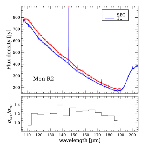
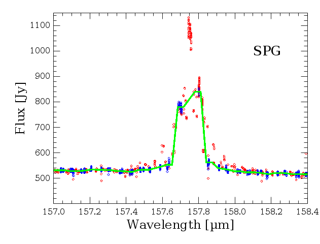
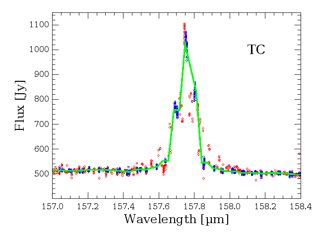
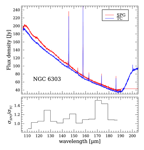
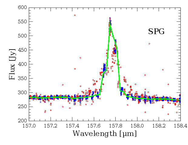
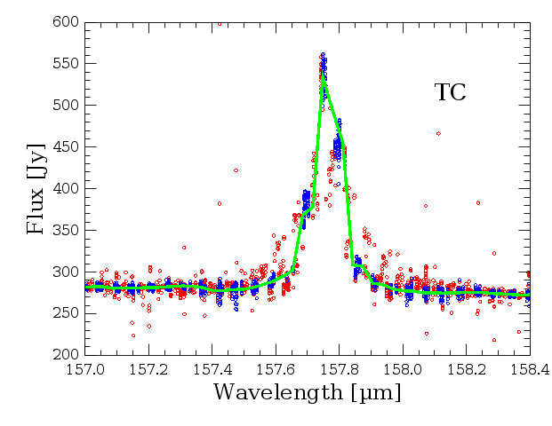
Figure 14: Left: Spectra of Mon R2 and NGC 6303 from the archive products (SPG, red) and reduced with our pipeline (TC, blue). Right: [CII] line as recovered by the SPG and TC pipelines for the two sources before background subtraction. Masked frames are shown as red points.

6.3 Mapping

Another effect due to the presence of transients in the data is clearly visible when considering raster maps. When examining the observation obsid 1342246963 (see Figure 15), we notice the presence of a transient all along the observation. In particular, the most affected part is the first off-target observation (blue points in the figure). If this transient is not corrected and the off-spectrum is computed by averaging the two off-target position spectra, the result is an off-target spectrum with fluxes typically greater than those of the on-target spectrum. For this reason, after the subtraction, the flux values are negative. Moreover, as shown in the figure, the transient affects the first half of the on-target observation. If this is not corrected, the result is a gradient in the final image. The improvement can be easily seen by eye at the bottom of Figure 15, where we compare the image at 122 $\mu$m without (left), and with (right), the application of the transient correction.

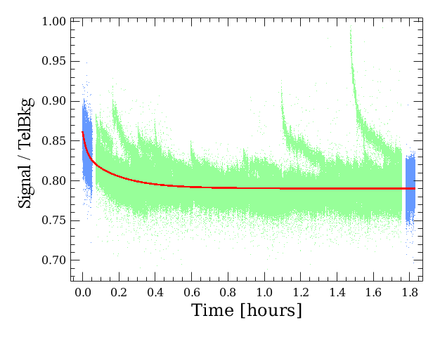
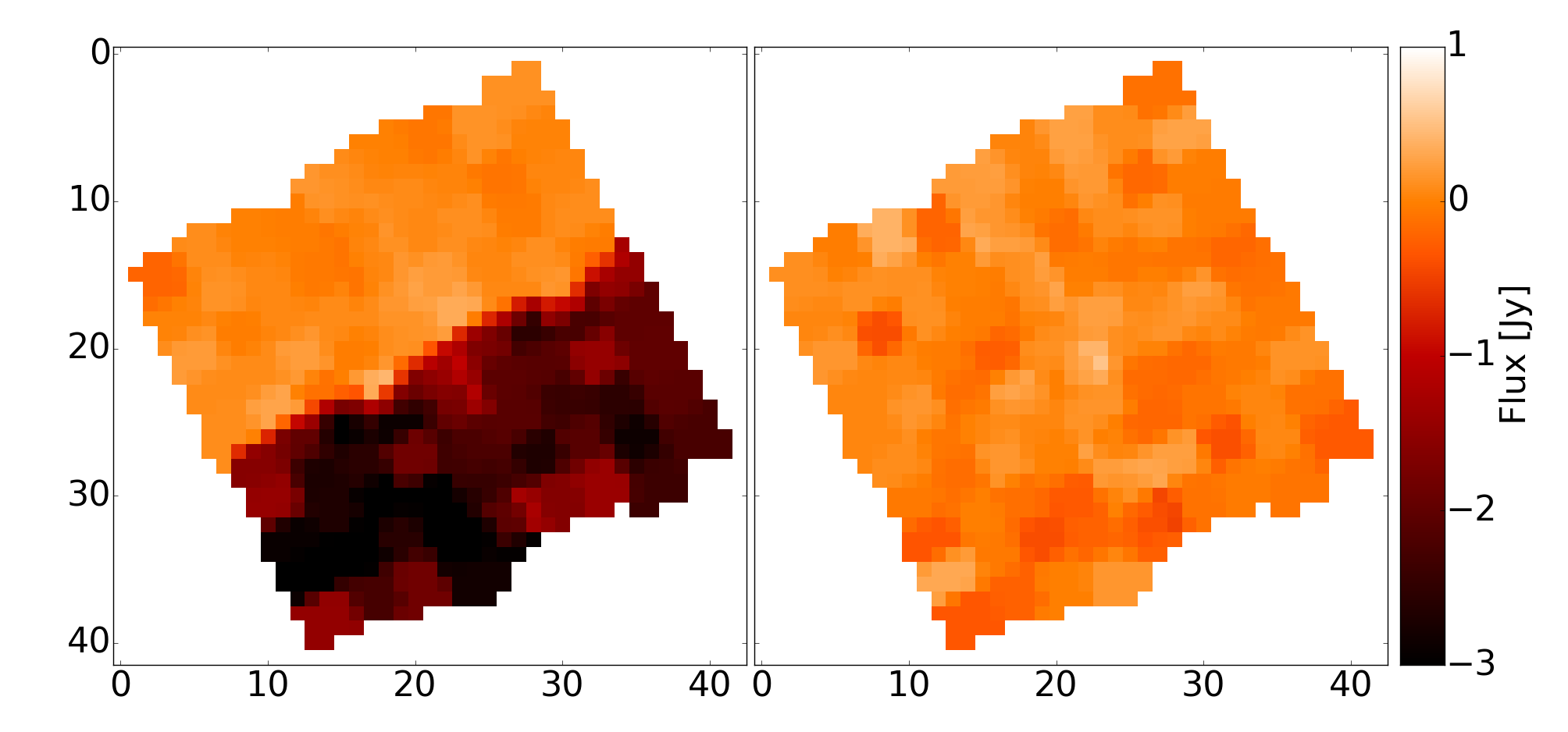
Figure 15: Top panel: long-term transient for the module 14 of the observation 1342246963. Blue and green points are frames taken off- and on-target. Bottom panels: Images at 122 $\mu$m as reduced by archive pipeline (left) and the interactive pipeline with transient correction (right). The huge transient in this 2$\times$2 raster observation causes, if not corrected, an uneven background with a negative flux in half of the archival image.

6.4 Direct comparison with chop-nod

In order to validate the transient correction pipeline release with version 14 of the HIPE software, a series of observations obtained with chop-nod and unchopped mode were compared. The comparison was limited to the features in the spectra, since the absolute value of the continuum cannot be obtained with the same accuracy as in the chop-nod mode. Only in the case of negligible signal from the source we can apply a general transient correction to the entire observation (see e.g. Figure 3). In all the other cases, strong continuum signals can affect the solution. In these cases, we cannot guarantee the accuracy of the absolute value of the continuum.

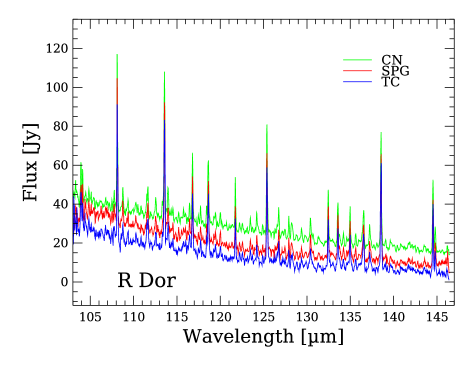
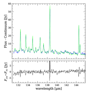
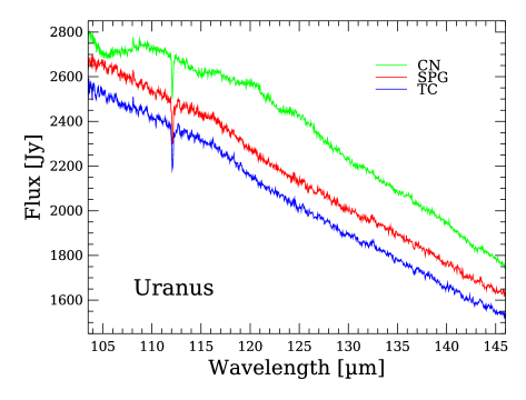
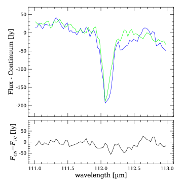
Figure 16: Comparison between spectra obtained with unchopped (red for SPG, blue for our pipeline) and chop-nod (green) modes for R Doradus and Uranus. The right panels show a comparison of emission and absorption lines in unchopped and chop-nod modes.

As a first example we considered the observations of the star R Doradus. The top left panel of Figure 16 compares the chop-nod (green, AOR 1342229701) with the unchopped data (AORs 1342229704/5) from the SPG pipeline (red) and our pipeline (blue). In the right panel, the reduction with the transient-correction pipeline is compared to the chop-nod data showing an excellent agreement. We notice that, thanks to the transient correction, the slope of the spectrum reduced with our pipeline is similar to that of the chop-nod observations, while the archival spectrum is steeper.

The second example considered is the planet Uranus, an extended source on the scale of the PACS spectrometer spaxels. We show in the bottom panels of Figure 16 the comparison between the chop-nod (AOR 1342257208) and unchopped observations (AORs 1342257211/2). Since the source is extended, we plotted the sum of the $3\times 3$ central spaxels. Probably because of pointing problems, the chop-nod data show a turn-around around 110 $\mu$m which is not present in the unchopped data and it is not predicted by models (see, for instance, Müller et al., 2014). Also in this case, when directly comparing the absorption feature of the spectrum, the match is very convincing.

7 Programs

In this section we describe the modules written to implement the various algorithms described in the previous sections, the two interactive pipelines available in the HIPE distribution for line and range observations, and the implementation of multi-threading for speeding up the data reduction which was introduced in HIPE for transient correction.

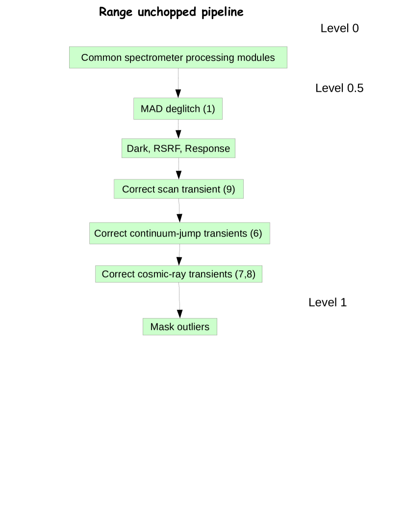
Figure 17: Flow-charts of the unchopped pipelines for the line and range modes (left and right, respectively). In the range mode the pipeline stops at level 1 products. In fact, two observations are required to complete the data reduction since the on-target and off-target observations are executed in different AORs. The numbers in brackets correspond to the tasks used for the step as described in section 7.1.

7.1 HIPE modules

Several tasks have been developed to implement the different algorithms described in the text. Their HIPE names with the numbers used in Figure 17 are:

1. specFlagGlitchFramesMAD

2. plotLongTermTransientAll

3. specLongTermTransientAll

4. specApplyLongTermTransient

5. plotTransient

6. specLongTermTransCorr

7. specMedianSpectrum

8. specTransCorr

9. specUpDownTransient

The complete description of these tasks is available in the section 6 of the PACS Data Reduction Guide for spectroscopy. The task specFlagGlitchFramesMAD replaces the deglitching task specFlagGlitchFramesQTest used in the chop-nod pipeline. The chop-nod task masks glitches and part of the resulting transient. In our case, we want to preserve these data to fit our transient model. We achieve this result by computing the local noise and masking only outliers beyond a given threshold. The task specLongTermTransientAll fits the transient along the whole history of the pixel (see Figure 3). The fits of transients during science blocks are performed by the task specLongTermTransCorr (see Figure 5). The task specMedianSpectrum evaluates the “Guess” spectrum (see Figure 6). An important bug in this task has been corrected in HIPE 15 (build no. 2845). Transients caused by cosmic ray hits are treated with the task specTransCor (see Figures 7 and 8). This task creates a new mask (UNCORRECTED) which contains the part of the signal which cannot be fitted by our model since the interval between two consecutive discontinuities contains less than 10 points. Finally, the correction of scan dependent transients described in section 5.4 is implemented in the task specUpDownTransient.

The unchopped transient correction pipelines make use of MINPACK, a robust package for minimization. MINPACK is more robust in its handling of inaccurate initial estimates of the parameter values than other conventional methods. We implemented MINPACK in HIPE as the “MinpackPro Least Squares Fitting Library”. This implementation is based on the original public domain version by Moré et al. (1980) . Our JAVA version is based on a translation to the C language by S. Moshier . MinpackPro contains enhancements borrowed from C. Markwardt’s IDL fitting routine MPFIT  (see also Markwardt, 2009).

7.2 HIPE pipelines

The flow-chart of the pipelines for the reduction of line and range unchopped data is shown in Figure 17. In the case of the line mode, one AOR contains the on- and off-target observations. So, the pipeline goes from the raw data to the final projected spectra. We suggest to set the parameter “interactive” to “True” in order to trigger the interactive step described in the flow-chart to check if the transient across the entire observation is correctable. This parameter is set to “False” in the script to allow for automatic checks of the pipeline during software updates.

In the case of the range mode, the main difference is the presence of the transient correction due to the rapid change of the telescope background during a wavelength scan. Also, the correction of the whole observation transient is not necessary since range-mode AOR contain only a on- or off-target observation. For this reason, the range-mode pipeline stops at level 1 products. To obtain level 2 products, one has to combine the reduction of the on- and off-target AORs using the “combine on-off” script available under the pipeline unchopped range scan menu.

7.3 Multi-threading

Since transient correction tasks are computationally intensive, we created the multi-threading framework ThreadByRange in HIPE to exploit the increasing availability of multiple cores in modern computers. This multi-threading framework takes advantage of the organization of the PACS data. In the pipeline, data are stored as Frames, i.e. time ordered sets of signal, wavelength, etc. for the 25$\times$16 pixels. Frames are then organized in blocks called Slices which correspond to the different parts of an observation (e.g. the calibration block, off-target observations, several raster positions, etc.). The correction tasks can run on each spaxel independently, so that it is possible to run 25 parallel processes. On the top of that, each Slice can be processed independently. Therefore, we organize the threads into two pools of threads for processing. One pool is for threads dedicated to processing the Slices, the other to operate on each spaxel. Resource usage can be controlled by specifying the pool sizes as task parameters. The default is to create two threads for processing Slices and a number of threads for the spaxels equal to half of the CPUs available.

The tasks implemented in HIPE require a combination of serial and parallel processes. Taking the signal from or applying the correction to Frames must be done serially, since the results of asynchronous updates to shared objects are undefined. Three methods are defined in ThreadByRange to interact with data:

• preApply() Initialization that must be done serially for the computational unit. In the case of pipeline tasks, this involves copying signal, wavelengths, masks, etc. to memory that is accessed exclusively by the apply() method.

• apply() ThreadByRange schedules this method to be applied in parallel. All of the work applied to spaxels in parallel is done here, such as minimizations, discontinuity detection, application of corrections, etc.

• postApply() ThreadByRange calls this method after the completion of each work unit. Transient correction tasks use this method to update Frames with the correction for each spaxel.

An absolute requirement for multi-threading is thread safety of the classes defined in the transient correction tasks. Fortunately, the level of thread safety was easy to determine due to the robust, clean design of the numerical package of HIPE.

Our multi-thread framework ThreadByRange sits on the Java Concurrency Package from which we use the JAVA ExecutorCompletionService for synchronization, and the Executors’ fixedThreadPool for scheduling. In the processing of spaxels or Slices, a Callable is created for each computational unit and is submitted to the CompletionService. This service synchronizes on task completion by using the BlockingQueue to retrieve completed tasks as Futures. For a complete description of the Java classes Callable, Executor, BlockingQueue, Futures, and of this mechanism see Goetz (2006, section 6.3.5 “Java Completion Service: Executor meets BlockingQueue”).

8 Summary and conclusion

We presented a description of transient effects on the response of the PACS spectroscopy detectors. Taking into account these effects is paramount in the case of observations using the unchopped modes. In fact, contrary to the chop-nod mode, there is no way to cancel these effects by constantly monitoring an off-target signal since on-target and off-target observations are made at different times.

We showed how it is possible to disentangle and treat separately transients due to different effects and how to improve dramatically the signal-to-noise ratio of the final products with respect to those from the Herschel archive. In particular, in the line mode the signal-to-noise ratio of lines can easily triple. In the case of range-mode, the correction of transients can lead to changes of slope, smoother spectra, and better reconstructions of bright lines. The algorithms described in the paper have been implemented in programs available in HIPE since version 14, as part of the drop-down menu for so-called interactive (ipipe) scripts. In particular, two different pipelines scripts are available for the reduction of line and range unchopped modes. An important bug affecting the range unchopped mode was corrected in HIPE version 15 (build 2845).