Efficient implementation of core-excitation Bethe-Salpeter equation calculations

Abstract

We present an efficient implementation of the Bethe-Salpeter equation (BSE) method for obtaining core-level spectra including x-ray absorption (XAS), x-ray emission (XES), and both resonant and non-resonant inelastic x-ray scattering spectra (N/RIXS). Calculations are based on density functional theory (DFT) electronic structures generated either by abinit or Quantumespresso, both plane-wave basis, pseudopotential codes. This electronic structure is improved through the inclusion of a GW self energy. The projector augmented wave technique is used to evaluate transition matrix elements between core-level and band states. Final two-particle scattering states are obtained with the NIST core-level BSE solver (NBSE). We have previously reported this implementation, which we refer to as ocean (Obtaining Core Excitations from Ab initio electronic structure and NBSE) [Phys. Rev. B 83, 115106 (2011)]. Here, we present additional efficiencies that enable us to evaluate spectra for systems ten times larger than previously possible; containing up to a few thousand electrons. These improvements include the implementation of optimal basis functions that reduce the cost of the initial DFT calculations, more complete parallelization of the screening calculation and of the action of the BSE Hamiltonian, and various memory reductions. Scaling is demonstrated on supercells of SrTiO₃ and example spectra for the organic light emitting molecule Tris-(8-hydroxyquinoline)aluminum (Alq₃) are presented. The ability to perform large-scale spectral calculations is particularly advantageous for investigating dilute or non-periodic systems such as doped materials, amorphous systems, or complex nano-structures.

1 Introduction

Core-level spectroscopies provide a quantitative element- and orbital-specific probe of the local chemical environment and the atomic and electronic structure of materials. For example, X-ray absorption (XAS) and emission (XES) spectra probe the unoccupied and occupied densities of states, respectively. The near-edge absorption region (XANES) is sensitive to oxidation state, spin configuration, crystal field, and chemical bonding, whereas the extended region can be used to reconstruct the local coordination shells. However, extracting this information requires a reliable interpretation of the measured spectra. Often this is done by comparison with reference spectra, but such comparisons are at best qualitative; it is preferable to calculate spectra quantitatively and predictively.

An accurate description of core-level excitations must take into account both the highly localized nature of the core hole and the extended condensed system. The problem of predictive computational x-ray spectroscopy has been approached from many directions, but most can be divided by scale into two major categories. Atomic and cluster models have sought to include a more exact treatment of many-body effects by considering a small subsystem coupled loosely or parametrically to the larger system. At the other end, various single-particle theories are able to treat many hundreds of atoms by approximating the electron-electron and electron-hole interactions. The utility of calculated spectra hinges upon compromises between the ability to accurately model a given system and the ability to address systems large enough to be representative of experiment: defects, dopants, interfaces, etc.

Within a first-principles approach, it is easiest to use the independent-particle approximation. For x-ray absorption, the extended region of materials is very well reproduced by the real-space Green’s function code feff, which is widely used over extensive energy ranges [1]. However, the current implementation loses accuracy at the edge when non-spherical corrections to the potential are important. To reproduce the near-edge structure, accurate independent quasi-particle models for deep-core XAS can be constructed for $s$-levels [2]. In this case, the x-ray absorption intensity is proportional to the unoccupied projected density of states in the presence of a screened core-hole, weighted by final-state transition matrix elements. This approach has been used with different treatments of the core-hole including the “Slater transition state” model of a half-occupied core state [3] or the final state picture of a full core hole with [4] or without [5] the corresponding excited electron. Due to the simplicity of their implementation and modest computational cost, such core-hole schemes have been implemented in several standard DFT distributions [6, 7, 8, 9, 10, 11, 12] for near-edge spectra. However, these approaches often fail when the hole has non-zero orbital angular momentum. Extensions to DFT such as time-dependent DFT (TDDFT) have been problematic due to the lack of sufficiently accurate exchange-correlation functionals for core-excited states. Although recent development of more accurate short-range exchange-corrected functionals [13, 14] has improved the viability of TDDFT for calculating core-level spectra more advances will be needed to make TDDFT a generally applicable approach.

The aforementioned approaches are all inherently single-particle descriptions. For calculating x-ray spectra this can be problematic, not only when the core hole has non-zero angular momentum, but also when many-body or multi-electron excitations are important. Many-electron wavefunction-based methods constitute one obvious approach to this problem. Contrary to single-particle descriptions that typically begin from the perspective of the extended system, atomic and cluster models start with the goal of completely describing the local problem. In particular, atomic multiplet theory [15] or configuration interaction [16, 17] and exact diagonalization methods [18] can accurately reproduce complicated L edges of transition metal systems. However, these techniques that take a local description typically ignore solid-state effects and are limited to small cluster models, although recent progress at incorporating band structure within the multiplet model should be noted [19, 20, 21].

Further improvements in DFT-based approaches to calculating spectra require a two-particle picture including particle-hole interactions, particle and hole self-energies, and full-potential electronic structure, within the context of many-body perturbation theory. Specifically, this involves solving the Bethe-Salpeter equation (BSE), i.e., a particle-hole Green’s function. The Bethe-Salpeter equation description of absorption includes single-particle terms that describe the quasi-particle energies of the core hole and the excited photoelectron, together with the interaction between them. To leading order the interaction consists of two terms: the Coulomb interaction, which includes adiabatic screening of the core hole, and an unscreened exchange term. Even this two-particle description of the many-body final state is already a significant improvement for L edges [22]. For example, when considering the L_2,3 edges of the transition metals, the independent-particle approximation predicts a 2:1 branching ratio between the intensities of the L₃ and L₂ edges, which is in contrast to experiments which exhibit branching ratios ranging from 0.7:1 for Ti to beyond 2:1 for Co and Ni [23, 24, 25, 26, 27, 28, 29]. The BSE largely resolves this discrepancy, yielding branching ratios in reasonable agreement with experiment [30]. However, simpler approaches such as TDDFT can also account for these corrections [31, 32, 33].

BSE solvers have been implemented in a few core-level codes to date [34, 35, 36] – as well as some valence level codes [37, 38, 39, 40] – but their utility has been limited to a specialist community. In part, this is due to significantly increased computational cost. feff and DFT-based core-hole approaches require little more effort than standard DFT calculations [41], and calculations on systems of hundreds of atoms have become routine. BSE calculations are considerably more intensive and have heretofore typically been limited to a few tens of atoms. This added cost is largely associated with including GW self-energy corrections to the electronic structure, obtaining the screening response to the core hole, and acting with the Bethe-Salpeter Hamiltonian on the electron-hole wavefunction to obtain the excitation spectrum. However, given the significantly improved accuracy of the BSE method it is desirable to make this a more widely used technique. This necessitates improving its ease of use and reducing the computational cost. Toward this second objective we report herein several efficiency improvements to our existing BSE code [42] that now allow BSE calculations on systems of hundreds of atoms and significantly reduce the time required for previously viable smaller systems.

The most time-consuming steps of a BSE calculation are (1) obtaining the ground-state electronic structure, (2) correcting the quasiparticle energies by adding a (GW) self-energy, (3) evaluating the screening response to the core-hole, and (4) determining the excitation spectrum of the BSE Hamiltonian. Our BSE calculations build on self-consistent field (SCF) DFT calculations of the ground-state charge density and the accompanying Kohn-Sham potential. We then use non-self-consistent field (NSCF) calculations, i.e., direct calculations that solve the one-electron Schrödinger equation in the already computed Kohn-Sham potential, to obtain all desired occupied and unoccupied Bloch states. To alleviate the burden of k-space sampling during the NSCF calculation, and to reduce the plane-wave basis, we implement a k-space interpolation scheme that solves a $k$-dependent Hamiltonian over a reduced set of optimal basis functions [43, 44]. This is described in section $3.1$. In most cases, rather than evaluating the GW self-energy in the typical random-phase approximation ($G^{0}W^{\text{RPA}}$), we instead use a much more computationally efficient approximation based on a multi-pole model for the loss function. This has been previously described in detail [45], and we will not discuss it further here. To reduce the time required to calculate the screening response to the core-hole we take advantage of the fact that this screening is highly localized around the excited atom and partition space accordingly. The electronic response is evaluated locally and a model dielectric response proves adequate for the rest of space [46]. Here we reduce the time needed to evaluate the screening response and action of the BSE Hamiltonian by parallelizing these portions of the code. This is discussed in section 3.2 for the BSE Hamiltonian and section 3.3 for the screening. In section 4 we demonstrate the effectiveness of these improvements through XAS calculations on a series of supercells of SrTiO₃. Section 4.1 characterizes the time-scaling of the code with respect to system size. Section 4.2 evaluates the savings realized by employing the optimal basis functions. The efficacy of parallelization is reported in section 4.3 for the action of the BSE Hamiltonian and in section 4.4 for the screening response. Example XAS and XES spectra of the commonly studied organic molecule Tris-(8-hydroxyquinoline)aluminum (Alq₃) are presented in section 4.5. We end with a summary of the capabilities of ocean and some general comments on its applicability.

2 Formalism

The theoretical description of the absorption of a photon by a material may be expressed in terms of the loss function $\sigma({\bf q},\omega)=-{\rm Im}\,\epsilon^{-1}({\bf q},\omega)$. The dielectric response function $\epsilon$ depends on the photon energy $\omega$ and the momentum transfer ${\bf q}$. A formal many-body expression for the loss function may be given as

$$\sigma({\bf q},\omega)\propto-\frac{1}{\pi}{\rm Im}\langle 0|\hat{O}^{+}G(\omega)\hat{O}|0\rangle,$$ (1)

where $|0\rangle$ is the many-body ground-state wavefunction, the operator $\hat{O}$ describes the interaction between the photon field and the system, and $G(\omega)$ is the Green’s function for the many-body excited-state. The form used for the operator $\hat{O}$ depends on the physical process being studied, e.g., $e^{i{\bf q}\cdot{\bf r}}$ for non-resonant inelastic x-ray scattering (NRIXS) or the expansion $(\hat{\bf e}\cdot{\bf r})+(i/2)(\hat{\bf e}\cdot{\bf r})({\bf q}\cdot{\bf r})+\dots$ for x-ray absorption (XAS); $\hat{\bf e}$ being the photon polarization vector. Using the Bethe-Salpeter Hamiltonian, the Green’s function for the excitation can be approximated in a two-particle form as

$$G(\omega)=[\omega-H_{\rm BSE}]^{-1}$$ (2)

where the Bethe-Salpeter Hamiltonian is typically given by

$$H_{\rm BSE}=H_{\rm e}-H_{\rm h}-V_{\rm D}+V_{\rm X}.$$ (3)

The term for the core-hole

$$H_{\rm h}=\epsilon_{\rm c}+\chi-i\Gamma$$ (4)

contains the average core-level energy $\epsilon_{\rm c}$, the spin-orbit interaction $\chi$, and the core-hole life-time $\Gamma$. In most practical work, the excited electron Hamiltonian

$$H_{\rm e}=H_{\rm KS}+\Sigma^{\it GW}-V_{xc}$$ (5)

is approximated by the Kohn-Sham Hamiltonian $H_{\rm KS}$ with a GW self-energy correction $\Sigma^{\it GW}$ where the exchange-correlation energy, $V_{xc}$, is subtracted off due to double-counting. The excited electron and hole interact via the Coulomb interaction within the mean-field of the remaining electrons. This is separated into the attractive direct term  

$$V_{\rm D}=\hat{a}_{\rm v}^{+}({\bf r},\sigma)\hat{a}_{\rm c}({\bf r^{\prime}},\sigma^{\prime})W({\bf r},{\bf r^{\prime}},\omega)\hat{a}_{\rm v}({\bf r},\sigma)\hat{a}_{\rm c}^{+}({\bf r^{\prime}},\sigma^{\prime}),$$ (6)

which is screened by the other electrons in the system, and the repulsive exchange term  

$$V_{\rm X}=\hat{a}_{\rm v}^{+}({\bf r},\sigma)\hat{a}_{\rm c}({\bf r},\sigma)\frac{1}{|{\bf r}-{\bf r^{\prime}}|}\hat{a}_{\rm v}({\bf r^{\prime}},\sigma^{\prime})\hat{a}_{\rm c}^{+}({\bf r^{\prime}},\sigma^{\prime}),$$ (7)

which is treated as a bare interaction. The $\hat{a}_{\rm v}^{+}$ ($\hat{a}_{\rm v}$) operator creates (annihilates) an electron in the valence level while $\hat{a}_{\rm c}^{+}$ ($\hat{a}_{\rm c}$) creates (annihilates) an electron in a core level.

Our implementation of the GW-BSE method is referred to as ocean (Obtaining Core Excitations from Ab initio electronic structure and NBSE) and we have previously presented it in detail [42]; NBSE refers to the NIST BSE solver. Because solving the Bethe-Salpeter equation at the level of approximation described above is computationally intensive compared to other methods of calculating x-ray spectra our approach makes several reasonable approximations to improve the efficiency of the calculation. Specifically, within a plane-wave approach to solving the Kohn-Sham equations, we use pseudopotentials to reduce the number of electrons and size of the plane-wave basis. The GW self-energy is obtained through the highly efficient many-pole self-energy approximation when appropriate [45]. The effort required to obtain the screening for the direct interaction is also reduced by utilizing a hybrid real-space approach in which the screening response is evaluated at the RPA level locally about the absorbing site, but the long range screening is approximated with a model dielectric function [46].

Despite these efficacious strategies, the largest system treated with our previous implementation of ocean was a water cell consisting of 17 molecules [47]. To extend the capabilities of ocean to treat larger systems we have made several improvements. A calculation with ocean consists of four stages

1. DFT  2. Translator  3. Screening  4. BSE

where stage 2 is a translation layer that allows different DFT packages to be used as the foundation for ocean.

The limiting points of the calculation previously were stages 1 and 3, solving the Kohn-Sham equations and evaluating the screening response to the core-hole. Stage 4, the actual evaluation of the Bethe-Salpeter Hamiltonian, was also a limiting point for systems that required sampling numerous atomic sites. Therefore, our efforts focused on (i) improving the efficiency of the DFT calculation and (ii) parallelizing the evaluation of the screening response and the Bethe-Salpeter Hamiltonian.

3 Implementation

3.1 Optimal Basis Functions

Our previous version of ocean used abinit [6, 7, 8, 9] as the DFT solver. ocean may now be alternatively based on wavefunctions obtained with Quantumespresso [10]. For the purpose of this paper, we report results based on the use of Quantumespresso rather than abinit, though either DFT solver may be chosen depending on the preference of the user.

The loss function in eqn. 1 is calculated by transforming the implied integral over all space into sums over reciprocal-space $\mathbf{k}$-points within the Brillouin zone and real-space $\mathbf{x}$-points within the unit cell, as is standard in calculations of periodic systems. The sum over $\mathbf{k}$-points requires a denser mesh for converging spectra than properties such as the density. Additionally, the BSE approach necessitates summing over a large number of unoccupied states which are also not needed when looking at ground-state properties. Thus, a considerable number of Kohn-Sham states must be constructed.

We reduce the computational cost of generating the Bloch functions through the use of optimal basis functions (OBF) [43]. We have implemented the OBF routines of Prendergast and Louie as a middle-layer in the ocean code [44]. The OBFs are a method of $\mathbf{k}$-space interpolation and basis reduction. A fully self-consistent DFT calculation is carried out to converge the density, using only enough bands to cover the occupied states. With this density a non-SCF calculation is performed, including unoccupied bands for the screening and BSE calculations (the density is held constant and the Kohn-Sham eigensystem is solved for all the bands needed for the BSE). This second calculation is used as a basis to create the OBFs. By using the OBFs we achieve a significant reduction in the time spent calculating the Bloch functions for a given system. Further details and quantitative results are presented in section 4.2.

3.2 BSE Hamiltonian

In ocean the BSE Hamiltonian acts on a space containing a core-level hole with index $\alpha$ and a conduction band electron with indicies $n,\mathbf{k}$. A vector in this space is described by the coefficients $\psi_{\alpha,n,\mathbf{k}}$, and the photoelectron wavefunction for a given core index $\alpha$ is easily expanded in real space from the conduction-band Bloch functions

$$|\Phi_{\alpha}(\mathbf{x},\mathbf{R})\rangle=\sum_{n,\mathbf{k}}\psi_{\alpha,n,\mathbf{k}}\,e^{i\mathbf{k}\cdot(\mathbf{R+x})}|u_{n,\mathbf{k}}(\mathbf{x})\rangle.$$ (8)

Within OCEAN we are interested primarily in the resulting x-ray spectrum, rather than obtaining the actual eigenvalues and eigenvectors of the Bethe-Salpeter Hamiltonian, and so the iterative Haydock technique is used [48, 49]. The advantage of an iterative technique is that the complete Hamiltonian does not need to be explicitly constructed or stored. Rather, at each step in the Haydock scheme the BSE Hamiltonian acts on the vector determined by the previous iteration,

$$\psi^{i+1}_{\alpha,n,\mathbf{k}}=H_{\text{BSE}}\,\psi^{i}_{\alpha,n,\mathbf{k}},$$ (9)

where $i$ gives the $i$th vector, and convergence of the spectrum can be achieved in only a few hundred iterations (true diagonalization requires a number of steps equal to the dimension of the matrix). A more explicit explanation is given by Benedict and Shirley in Ref.  49. We divide up equation 9 by separating the BSE Hamiltonian into pieces, each of which is evaluated in its ideal or most compact basis. This is outlined in the following two sections. The full vector $\psi^{i+1}$ is then the sum of contributions from each piece.

3.2.1 Long-range

Only the direct interaction has a long-range component as the exchange term requires both $\mathbf{r}$ and $\mathbf{r^{\prime}}$ be at the core-hole site. The screened-coulomb interaction can be expanded in spherical harmonics and separated by angular momentum $l$,

$$W(\mathbf{r},\mathbf{r}^{\prime}) =\int\!\!d\mathbf{r}^{\prime\prime}\frac{\epsilon^{-1}(\mathbf{r},\mathbf{r}^{\prime\prime})}{|\mathbf{r}^{\prime\prime}-\mathbf{r}^{\prime}|}=\sum_{l=0}^{\infty}W_{l}(\mathbf{r},\mathbf{r}^{\prime}).$$ (10)

The long-range part includes only the $l=0$ term,

$$W_{0}(\mathbf{r},\mathbf{r}^{\prime}) =\int\!\!d\mathbf{r}^{\prime\prime}\frac{\epsilon^{-1}(\mathbf{r},\mathbf{r}^{\prime\prime})}{\left[r_{>}\right]_{\mathbf{r}^{\prime\prime},\mathbf{r}^{\prime}}},$$ (11)

that goes as $1/r$ away from the core hole. All higher $W_{l}$ are treated as short ranged. By integrating out the core-hole dependence via the core-hole density $\rho_{\alpha}$

$$W_{0}(r) =\int\!\!d\mathbf{r}^{\prime}\rho_{\alpha}(\mathbf{r}^{\prime})\int\!\!d\mathbf{r}^{\prime\prime}\frac{\epsilon^{-1}(\mathbf{r},\mathbf{r}^{\prime\prime})}{\left[r_{>}\right]_{\mathbf{r}^{\prime\prime},\mathbf{r}^{\prime}}},$$ (12)

the long-range component of the BSE Hamiltonian is a function of the electron spatial coordinate only.

We evaluate the action of $W_{0}$ on a vector by first transforming to a super-cell space

$$\phi_{\alpha}(\mathbf{x},\mathbf{k}) =\sum_{n}\psi_{\alpha,n,\mathbf{k}}\,e^{i\mathbf{k}\cdot\mathbf{x}}|u_{n,\mathbf{k}}(\mathbf{x})\rangle$$ (13)

$$\phi_{\alpha}(\mathbf{x},\mathbf{R}) \equiv\mathcal{F}_{\mathbf{k}\rightarrow\mathbf{R}}[\phi_{\alpha}(\mathbf{x},\mathbf{k})],$$

where $R$ are the lattice vectors and $\mathcal{F}$ indicates a Fourier transform. The core-hole index $\alpha$ can refer to different angular momentum and spin $lm\sigma$ states of the core hole, but the long-range component of the direct term does not mix spin or angular momentum, and so these are treated sequentially. The $\mathbf{k}$-space grid used in an ocean calculation defines a maximum range of the screened core-hole potential.

Algorithm 1 Computing $\psi^{i+1}=W_{0}\psi^{i}$

1:for each $x$ and $\alpha$ do

2:     $\phi(\mathbf{k})=\sum_{n}\psi_{n,\mathbf{k},\alpha}^{i}\,e^{i\mathbf{k}\cdot\mathbf{x}}u_{n,\mathbf{k}}(\mathbf{x})$

3:     $\phi(\mathbf{R})=\mathcal{F}_{\mathbf{k}\rightarrow\mathbf{R}}[\phi(\mathbf{k})]$

4:     $\phi(\mathbf{R})=W(\mathbf{x},\mathbf{R})\times\phi(\mathbf{R})$

5:     $\phi(\mathbf{k})=\mathcal{F}_{\mathbf{R}\rightarrow\mathbf{k}}[\phi(\mathbf{R})]$

6:     $\psi_{n,\mathbf{k},\alpha}^{i+1}\mathrel{+}=\phi(\mathbf{k})\,e^{-i\mathbf{k}\cdot\mathbf{x}}u^{*}_{n,\mathbf{k}}(\mathbf{x})$

7:end for

The operation $\psi^{i+1}=W_{0}\psi^{i}$ is laid out in algorithm 1. Since the direct interaction is diagonal in real-space this procedure is easily parallelized by distributing the $\mathbf{x}$-points among all the processors. The parallel algorithm has the additional final step of summing the vector $\psi^{i+1}$ over all the processors. This limits the scaling, but the vector itself is not large. Both the number of $\mathbf{x}$-points and the number of empty bands required for a given energy range scale as the volume of the system.

3.2.2 Short-range

The short-range components of the Hamiltonian are calculated by projecting the conduction-band states into a local basis around the core hole. These basis functions have a well-defined angular momentum around the absorbing atom and are reasonably complete such that near the atom

$$\varphi_{n,\mathbf{k}}(\mathbf{r})|_{r<r_{c}}=\sum_{\nu,l,m}A_{n,\mathbf{k}}^{\nu,l,m}R_{\nu,l}(r)Y_{l,m}(\hat{r}).$$ (14)

$Y_{l,m}$ are the usual spherical harmonics and, following the ideas of the projector augmented wave method, $R_{\nu,l}$ are taken to be solutions to the isolated atom [50, 51]. This both allows us to capture the correct, oscillatory behavior of the valence and conduction states near the core-hole and gives us a compact basis for calculating the matrix elements of the short-range direct and exchange interactions. In practice, our core-hole will typically have 1 (s) or 3 (p) angular momentum states, and our conduction electrons will have 4 projectors each for $l=s,\cdots,f$ or 64 lm states. For an L edge this gives a maximum matrix dimension of $4\times 3\times 64=768$, including spin degrees of freedom for both the electron and the hole. This is completely independent of the overall system size.

The time-consuming steps in computing the short-range interactions are projecting into and out of the localized basis which requires summing over all of the bands and $\mathbf{k}$-points. The mapping of band states to localized states is precomputed and stored. We expand the exchange and local direct by angular momentum and exploit selection rules to limit the number of multipole terms. The various pieces of the short-range Hamiltonian are distributed to different processors. The small number of multipole terms and size disparity between them limits the degree of parallelization, but alleviates the need for a communication step. Each processor adds its results for the long- and short-range interactions, and then a single synchronizing summation of $\psi^{i+1}$ is carried out.

3.3 Screening

In the direct interaction the core-hole potential is screened by the dielectric response of the system. We calculate this response within the random phase approximation (RPA)

$$\chi^{0}(\mathbf{r},\mathbf{r}^{\prime},\omega)=\int\!\!\frac{\,d\omega^{\prime}}{2\pi i}G(\mathbf{r},\mathbf{r}^{\prime},\omega^{\prime})G(\mathbf{r}^{\prime},\mathbf{r},\omega^{\prime}-\omega).$$ (15)

We evaluate this expression in real-space around the core-hole, and, taking advantage of the localized nature of near-edge core excitations, we limit our full calculation to a sphere with a radius of approximately $r=8$ a.u., splicing on a model dielectric function for the long-range behavior [46]. The cross-over radius from RPA to model is a convergence parameter so that for each material one may ensure that this approximation has no discernible effect on the calculated spectra. We use static screening $\omega=0$ which assumes that the exciton binding energy is small compared to the energy scale for changes in the dielectric response, i.e., smaller than the band gap.

Our real-space grid is 900 points determined from a 36 point angular grid and 25 uniformly spaced radial points. We carry out the integral over energy in eqn. 15 explicitly along the imaginary axis, and for large systems the bulk of time is spent projecting the wavefunctions onto this grid and constructing the Green’s function

$$G(\mathbf{r},\mathbf{r}^{\prime},\mu+it)=\sum_{n,\mathbf{k}}\frac{\psi_{n,\mathbf{k}}(\mathbf{r})\psi^{*}_{n,\mathbf{k}}(\mathbf{r}^{\prime})}{\mu+it-\epsilon_{n,\mathbf{k}}},$$ (16)

where $\mu$ is the chemical potential. Using the OBFs, we determine the Bloch functions on the spherical grid and distribute the calculation across processors by dividing up the spatial coordinates. On modern computer architectures this operation will be limited by memory bandwidth. To alleviate this we have each processor work on one or more small blocks of the Green’s function such that we can be confident that the block will remain in the cache during the summation over bands.

To gain an additional level of parallelization we can also distribute the calculation by $\mathbf{k}$-point. We divide the total processors into pools of equal size, and every pool calculates $G_{\mathbf{k}}$. The sum $G=\sum_{\mathbf{k}}G_{\mathbf{k}}$ is carried out across the pools, placing the complete $G$ on the master pool. Then each processor in the master pool calculates $\chi^{0}$ via equation 15, performing the integral over the imaginary energy axis for its blocks. Finally, the complete matrix $\chi^{0}$ is written to disk. In practice, a $2\times 2\times 2$ shifted $\mathbf{k}$-point grid is used for screening calculations, giving 8 unique points in the Brillouin zone and allowing up to 8 pools. There is some cost to performing the parallel sum of $G$ over pools and inefficiency in evaluating $\chi^{0}$ on only the master pool, however neither of these contribute significantly to the running time.

Table 1: Timing budget variation with system size. The central portion of the table lists the total run-time in minutes spent on each stage of the calculation. The DFT portion of the calculation was performed in parallel and the time shown is the run-time multiplied by the number of cores used. The remaining stages were carried out on a single core.

	Supercell (N)	1	2	3	4
	Rel. System Size	1	8	27	64
	DFT	22	832	17161	265226
	Translator	0.08	2.5	43.8	754
	Screening	0.2	2.0	15.4	76.5
	BSE	0.5	26.1	250	1915

4 Results

To demonstrate the scaling performance of ocean we consider the Ti L-edge XAS of supercells of SrTiO₃. Pure SrTiO₃ is a wide band-gap semiconductor and incipient ferroelectric that assumes an undistorted cubic structure at ambient conditions. SrTiO₃ is a foundational material on which a remarkable variety of electronic and opto-electronic devices are based. Epitaxially interfacing SrTiO₃ with other oxide compounds, notably LaAlO₃, can yield interfacial 2-dimensional electron gases that are good conductors [52], superconducting [53], show magnetic ordering [54], or that are even simultaneously superconducting and magnetically ordered [55, 56]. Doping SrTiO₃ also produces a wide range of useful physical properties. Addressing these interesting systems numerically requires the use of large supercells. For instance, a doping level of 3.7 $\%$ (1/27) necessitates a $3\times 3\times 3$ supercell while for a 1.56 $\%$ (1/64) doping level a $4\times 4\times 4$ supercell must be constructed.

In this section we consider run-times for cubic supercells of pure SrTiO₃ with N = $\{1,2,3,4\}$ repetitions of the conventional cell in each direction. This corresponds to systems with $\{5,40,135,320\}$ atoms and $\{32,256,864,2048\}$ valence electrons, respectively. We begin in section 4.1 with benchmark calculations by investigating the single-core time-scaling of the original screening and BSE portions of the calculation. The four supercells are run with equivalent parameters and the usual basis of Kohn-Sham orbitals, that is, without employing the optimal basis functions. We next consider in section 4.2 the savings gained through the k-space interpolation scheme of optimal basis functions. In sections 4.3 and 4.4, we determine the scaling behavior of the parallel implementation of the BSE and screening routines, respectively. We end in section 4.5 with a brief demonstration of ocean by calculating the x-ray absorption and emission spectra of an organic molecule commonly used in light emitting diode devices.

4.1 Single Processor Calculations

Before discussing the improvements we have made it is informative to establish the prior baseline performance of ocean. We performed a series of timing tests for which the DFT portion of the calculation was executed in parallel over a given number of cores while the remaining stages of the calculation used only a single core. We use the Quantumespresso density-functional theory package to generate the ground-state electronic structure upon which the spectral calculations are based. These calculations are performed with norm-conserving pseudopotentials obtained from the abinit distribution [6, 7, 8, 9] with the exception of Ti for which we made a pseudopotential with semi-core states included in the valence configuration. We employ the local-density approximation to the exchange correlation functional and truncate the planewave basis at 50 Ry. $\Gamma$-point sampling was used to obtain the ground-state electron density, which was subsequently expanded into separate sets of Kohn-Sham orbitals for the evaluation of the screening and the Bethe-Salpeter Hamiltonian. In each case, the number of empty bands utilized equaled the number of occupied bands. For the screening response, states were constructed at a single k-point while to evaluate the Bethe-Salpeter Hamiltonian states were expanded on a shifted $2\times 2\times 2$ grid. The above values were sufficient for convergence of the final spectrum for supercells with N $\geq$ 2. Since our purpose at present is to study the scaling performance of ocean we use these same values for the N = 1 case (conventional cell) even though this k-point sampling is insufficient for convergence at this size. (Convergence at N = 1 can be reached by increasing the k-point sampling to $2\times 2\times 2$ for the density and evaluation of the screening, and to $3\times 3\times 3$ for the BSE.)

Table 1 reports the timing budget separated by stage of the calculation for each of the four supercells. The DFT segments of the calculations were run in parallel and the time reported is the product of the run-time and the number of cores used. The remaining stages of the calculation were all run on a single core; only a single Ti site was interrogated for each supercell. Extrapolating these times to all Ti sites in each supercell, we find that the run-time required for the three stages after the DFT portion constitutes approximately 30 $\%$ of the total calculation time for the larger supercells. Parallelization of these segments could then reduce their run-time to a small fraction of the DFT run-time. Table 1 shows that the time spent in the BSE stage dominates that used in the screening portion of the calculation. Thus, it is essential to implement an effective parallelization scheme for the BSE stage; this will be demonstrated below. The wavefunction translation step also becomes time consuming for large systems. At present, we have not sought to improve the efficiency of this process, but future efforts may be directed at reducing the time required here.

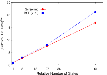
Figure 1: Run-Time Scaling. The relative run-times for the screening and BSE portions of the calculation are presented versus system size. The screening (left axis, red circles) scales with the system size to the second power and the BSE (right axis, blue squares) goes as the system size to the fourth power.

The individual run-time scaling of the screening and BSE stages of the calculation are presented in Figure 1. These results demonstrate that both the screening calculation and the evaluation of the BSE scale as the number of states to the second power. Since we use the same k-point grids for all supercells the variation in the number of states comes from the increasing number of bands which grows proportionally with the supercell size. In this example we have considered a single site in the super cell. The number of sites also grow with volume, leading to an overall scaling of volume cubed for both the screening and BSE. Given that as the system size increases the BSE stage comes to dominate the overall run-time, it is clearly advantageous to find an effective parallelization scheme for this stage. This is discussed below in section 4.3.

From eqn. 16 it appears that the screening calculation should scale directly with the number of bands as the radial grid is independent of system size. However, for large systems much of the time is spent projecting the DFT wave functions onto the radial grid from the planewave basis. Both the number of planewaves and bands grow with system size leading to this second power behavior. This indicates that an improved approach to projecting the Kohn-Sham states onto the local basis is an avenue to further reducing the time spent in the screening routine.

Per section 3.2, the BSE Hamiltonian is broken into three sections: non-interacting, short-range, and long-range. The non-interacting term is diagonal, and, for a single site scales directly with system size. The short-range part, like the screening calculation, relies on a small, localized basis that does not change with system size. Also like the screening calculation, for large system the projection of the DFT orbitals into this localizated basis to determine the coefficients $A$ (eqn. 14) will grow with both the number of planewaves and bands. While this projection happens only once at the beginning of the BSE stage, it does lead to scaling with the second power of the system size. The long-range part of the BSE is the most computationally expensive. As shown in algorithm 1, the action of $W_{0}$ grows with both the number of x-points and the number of empty states, both of which scale linearly with system size. Therefore the BSE section of the code is expected to scale with the second power of system size, as is confirmed in figure 1.

4.2 Reduced Basis

For the SrTiO₃ supercells presented in this work, $\Gamma$ point sampling was used as an input to the OBF scheme and the Bloch functions were interpolated onto $2\times 2\times 2$ $\mathbf{k}$-point grids (For the single cell a $2^{3}$ $\mathbf{k}$-point grid was interpolated to a $3^{3}$ grid). As NSCF DFT calculations scale linearly with the number of $\mathbf{k}$-points this represents a potential 8x speedup (3.4x for the conventional cell). This gain, however, is partially offset by the additional steps needed to carry out the OBF interpolation.

Table 2: The relative time required for each step in generating Bloch functions and the speedup with respect to the total run time achieved by using the OBFs (The total run-time includes steps not explicitly listed in the table).

	Supercell (N)	1	2	3	4
	Rel. System Size	1	8	27	64
	# Processors	8	32	64	128
	SCF	0.48	2.20	6.45	42.5
	NSCF	0.06	0.38	7.11	38.6
	OBF	0.18	1.55	12.1	49.7
	Total	1.00	4.90	30.3	152
	Speedup	1.27x	1.22x	2.24x	2.46x

In Table 2 we show the relative time for the SCF, NSCF, and OBF stages that are needed to generate Bloch functions for the BSE calculation. By assuming that the NSCF would necessarily take 8x (3.4x) longer without the OBF interpolation we estimate the savings as a percentage of the total run-time. While the small cells show only a modest improvement, the $3^{3}$ and $4^{3}$ cells complete in less than half the time when using the OBF scheme. Generically, the expected savings will depend most strongly on the needed $\mathbf{k}$-point sampling for the system under investigation. Metallic systems require much denser $\mathbf{k}$-point grids for convergence and will yield correspondingly larger savings.

4.3 BSE Scaling

To investigate the scalability of our parallel BSE solver with processor number we focus on the $4\times 4\times 4$ supercell of SrTiO₃. This system approaches the limits of single node execution due to memory considerations. A significant amount of time for each run is spent reading in the wavefunctions. For this example the wavefunctions require 12 GB of space (3072 conduction bands, 8 ${\mathbf{k}}$-points, and 32,768 ${\mathbf{x}}$-points). The time needed to read these data typically ranged from 40-60 seconds [57]. Currently, the wavefunctions are read in by a single MPI task and then distributed so this time is relatively constant with processor count. To give a better picture of the scaling, we subtract out the time required for this step before comparing runs. If multiple runs are carried out on the same cell, varying atomic site, edge, or x-ray photon (polarization or momentum transfer), the wavefunctions are kept in memory, and therefore this upfront cost will be amortized over all the calculations. In the present example we calculate the spectra for three polarizations, using 200 Haydock iterations.

To assess the scaling of the BSE section we use the metric cost. The cost reflects what the user would be charged on a computing facility: the run-time multiplied by the number of processors. A perfectly parallelized code would maintain a cost of 1.0 when run across any number of processors. Costs less than 1.0 would indicate some superscaling behavior, most likely from accidental cache reuse. In figure 2 we show the relative cost of the BSE section as a function of the number of processors. The testbed for this section consists of identical, dual socket nodes with 6 processors (cores) per chip and connected via high-speed interconnects. Each multi-node test was run five times and the best time for each was used.

The BSE section is a hybrid MPI/OpenMP code so we compare execution with various levels of threading. As can be seen in figure 2, the use of threads improves the speed of the calculation over pure MPI. This is true even when 12 threads are used, requiring communication across the two sockets via OpenMP. We also see very acceptable scaling with processor count. The benchmark calculation takes a little over 8.5 hours on a single node and single thread, while running on 192 cores can be done in approximately 3.5 minutes for a real-world speedup of 114x.

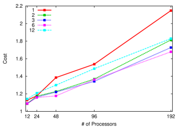
Figure 2: BSE Cost. The cost, ratio of actual run-time to theoretical linear scaling, as a function of processor count. Each line represents a different number of threads per node. One or two MPI tasks per socket (6 or 3 threads) are seen to give the best performance.

Sublinear scaling, a cost in excess of $1.0$, is, in general, the result of non-parallelized sections of code, synchronization costs, and memory bandwidth constraints. With the exception of the aforementioned wavefunction initialization, the BSE code has very little explicit serial execution. Further work is needed to investigate and alleviate the bottlenecks preventing linear scaling.

4.4 Core-hole Screening Scaling

In this section we investigate the timing of calculating the valence electron screening of the core-hole. As stated before, for core-level spectroscopy we are mainly interested in the local electronic response. Limiting our calculation of the RPA susceptibility to a region of space around the absorbing atom makes the calculation much cheaper than traditional planewave approaches without sacrificing accuracy [46]. Within this approach, and for most other methods of calculating core-excitation spectra, a separate screening calculation is required for each atomic site. In systems with inequivalent sites due to differences in bonding, defects, or vibrational disorder contributions from each atom must be summed to generate a complete spectrum.

To test the behavior of the screening section we use the same test case as for the BSE, the $4\times 4\times 4$ supercell of SrTiO₃. The RPA susceptibility is calculated using a single $\mathbf{k}$-point and 4096 bands. We show results for a single site, 16 sites, and 32 sites (out of the 64 titanium atoms in our supercell). The number of sites will vary based on the system being investigated. Impurities may require only a single site, but liquids or other disordered systems necessitate averaging over many sites [47, 58]. As is evident in figure 3, this section of the calculation does not scale beyond a few dozen processors. This is especially true when only investigating a single site. While better scaling is desirable, as observed in Table 1 the total time for this section is quite small. In this particular test the screening calculation took just under 8 min for a single site while the initial DFT calculations required approximately 3 hours on 128 processors.

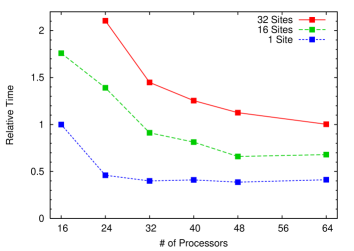
Figure 3: Screening scaling. The relative time for the screening section as a function of the number of processors. We show both the total time required for a single site, 16 sites, and 32 sites relative to the time needed to run the single site on 16 processors. The per site time is lower with a larger number of sites due to amortization of i/o and other initialization costs. While the scaling with processor number is poor, we see only very limited detrimental effects from using more processors, and therefore the screening calculation is run using the same processor count as the other stages.

4.5 Example Spectra

Figure 4 presents the Ti L edge of pure SrTiO₃ calculated for both the primitive cell (one formula unit) using our previous version of ocean [42] and for the $5\times 5\times 4$ supercell (100 formula units) obtained with the code improvements described herein. This comparison serves to verify that the fidelity of the computational scheme has been preserved through the modifications we have made and demonstrates the feasibility of calculating spectra of much larger systems than previously possible. Doping SrTiO₃ yields a wide range of interesting physical properties and we imagine that in future investigations it will be fruitful to apply ocean to studies of such systems. Compounds of SrTiO₃ doped with transition metals are investigated for use in photocatalysis and as permeable membranes, among other uses. Further, there is some evidence that doping with Mn, Fe and Co may yield dilute magnetic semiconductors [59, 60, 61]. The task of improving the performance of such materials is assisted by a better understanding of how the dopant element interacts with the host system. It is now possible to model such spectra with a realistic, first-principles approach.

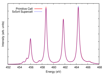
Figure 4: Ti L-edge XAS of SrTiO₃. Comparison of the Ti L-edge XAS of SrTiO₃ calculated from the primitive cell using abinit and the serial version of ocean and from the $5\!\times\!5\!\times\!4$ supercell using the OBFs and parallelized ocean code.

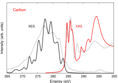
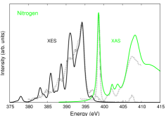
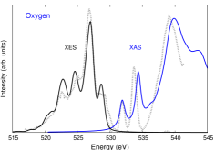
Figure 5: XAS and XES of Alq₃. K-edge XAS (color) and XES (black) of carbon (left, red), nitrogen (middle, green) and oxygen (right, blue) for gas-phase meridional Tris-(8-hydroxyquinoline)aluminum (Alq₃). Grey curves show the experimental data reproduced from reference [62].

As a second example system we consider the organic molecule Tris-(8-hydroxyquinoline)aluminum (Alq₃). Alq₃ has remained a leading molecule for the electron transport and emitting layer in organic light emitting devices since it was first proposed for this purpose [63]. Despite numerous academic and industrial investigations of such systems, significant problems remain, particularly regarding device lifetime. The Alq₃ molecule is susceptible to decomposition through reaction with water molecules [64] or metal atoms from the cathode layer [65, 66]. X-ray spectroscopy is commonly used to further reveal the interaction of water or metal ions with the Alq₃ molecule and the pathway by which the complex decomposes. However, results are difficult to properly interpret because such experimental work is rarely coupled with calculated spectra and because the molecule is sensitive to decomposition due to x-ray beam exposure. In this section we demonstrate the ability of ocean to produce reliable XAS and XES spectra for this system.

Alq₃ exhibits two isomers, commonly referred to as facial and meridional. The meridional isomer is favored energetically and we consider only this structure. In figure 5 we present the C, N and O K-edge XAS and XES from the meridional Alq₃ molecule, which consists of 52 atoms. We treat the molecule in the gas-phase, though devices typically contain amorphous films of the molecule. Since thermal atomic motion can noticeably impact spectral features for lighter elements we sum spectra from a series of configurations generated by a molecular dynamics (MD) simulation. The spectra presented in figure 5 show the average produced from 10 configurations of a MD simulation performed at 300 K within Quantumespresso. In addition to averaging over the MD configurations, each spectrum is an average over each atomic site in the molecule for the given element. Thus, these results represent a series of 30 calculations for the N edge, 30 calculations for the O edge, and 270 calculations for the C edge (keeping in mind that the same ground state DFT calculation can be used for all edges of a given MD configuration). Despite the large sampling required to produce these spectra the calculations are not particularly burdensome. After averaging over all samples and sites, self-energy corrections to the electronic structure were incorporated within the multi-pole self-energy scheme of Kas et al.  [45]. Finally, an ad hoc rigid energy shift was applied to each spectrum to align the absolute energies with the experimental values.

Our calculations are generally in good agreement with the measured spectra of Ref. [62]. The primary structure of the XAS is reproduced for each element with only a few minor differences. For carbon, the feature near 289 eV in our calculation appears in the experiment around 288 eV while, for nitrogen, the second feature is about 0.5 eV too low in energy in the calculation. The three peaks of the oxygen XAS match the experimental spectrum quite closely. The minor differences could originate in differences in electronic structure between the gas-phase, as we consider, and the condensed-phase material probed in experiment. Additionally, we presently neglect vibronic coupling in the excited-state [67, 68, 69] which can be particularly important in molecules with light elements [70, 71]. Nevertheless, agreement with experiment is generally quite favorable.

5 Conclusion

We have implemented a series of improvements that allow core-level spectral calculations based on solving the Bethe-Salpeter equation to be performed for much larger systems than previously possible. Whereas ocean was previously limited to systems of a few tens of atoms, here we have reported calculations on systems as large as a 5x5x4 supercell of SrTiO₃, which consists of 500 atoms and 3200 valence electrons and would allow for the direct simulation of doping at the 1 % level. This particular calculation required only 12.5 hours on 128 cores. This enhanced capability makes spectral calculations on amorphous and dilute systems feasible.

We reduced the cost of the non-self consistent field DFT calculation through a k-space interpolation scheme based on a reduced set of optimal basis functions. This yielded a speed-up by a factor of 2-2.5 for large systems. Parallelization of the screening calculation and evaluation of the BSE Hamiltonian provided further savings. We find that the parallelization of the screening response scales only to a few dozen processors. However, since the evaluation of the screening at this level of parallelzation has a limited cost compared to the initial DFT calculation this is not a significant concern at present. The BSE section of the code scales well to a few hundred processors with only a small growth in overhead that appears linear in processor count. When both MPI and OpenMP parallelization is used we achieved a speedup of 114x on 192 processors. However, when only MPI is used there is evidence that the overhead is growing superlinearly. There remains room for future improvement to reduce the MPI overhead.

In addition to x-ray absorption spectra and x-ray emission spectra, inelastic x-ray scattering spectra may also be calculated with ocean. We view ocean as uniquely capable of evaluating such spectra, particularly at L edges, with ab initio accuracy and predictive ability for complex and dynamic systems. We envision use of ocean to interpret data collected on a wide range of systems including in operando studies of fuel cell materials, photocatalysts, gas sensor and energy storage materials, as well as from liquid environments.

One should keep in mind that the Bethe-Salpeter equation is one of several approaches to calculating x-ray spectra. While the BSE method holds advantages in being a predictive, first-principles approach, its two-particle formulation, in certain cases, is still a crude approximation to the actual many-body problem. Contrary to this, many-particle approaches such as multiplet calculations and cluster models capture many-body physics more completely, though typically at the cost of band-structure effects. The challenge for these local methods is to incorporate the electronic structure of the extended system in a scalable fashion. It appears possible to make considerable progress toward this goal by working within a localized basis constructed from an extended electronic structure [19]. For the BSE technique, it will be necessary to incorporate additional many-particle effects. We expect that a better description of self-energy effects being made accessible by recent cumulant expansion development will prove advantageous in this respect [72, 73].

The ocean source code is now available for general use; for details and documentation see [74].

6 Acknowledgments

This work is supported in part by DOE Grant DE-FG03-97ER45623 (KG, JJK, FDV, JJR). KG was additionally supported by the National Natural Science Foundation of China (Grant 11375127), the Natural Science Foundation of Jiangsu Provence (Grant BK20130280) and the Chinese 1000 Talents Plan. Calculations were conducted with computing resources at Lawrence Berkeley National Laboratory and the National Energy Research Scientific Computing Center (NERSC), a DOE Office of Science User Facility supported by the Office of Science of the U.S. Department of Energy under Contract No. DE-AC02-05CH11231.

Certain software packages are identified in this paper to foster understanding. Such identification does not imply recommendation or endorsement by the National Institute of Standards and Technology, nor does it imply that these are necessarily the best available for the purpose.

References

- [1] J. J. Rehr, J. J. Kas, M. P. Prange, A. P. Sorini, Y. Takimoto, F. Vila, Comptes Rendus Physique 10 (2009) 548.
- [2] J. J. Rehr, A. J. Soininen, E. L. Shirley, Physica Scripta T115 (2005) 207.
- [3] L. Triguero, L. G. M. Pettersson, H. Agren, Physical Review B 58 (1998) 8097.
- [4] D. Prendergast, G. Galli, Physical Review Letters 96 (2006) 215502.
- [5] P. Rez, J. R. Alvarez, C. Pickard, Ultramicroscopy 78 (1999) 175.
- [6] The abinit code is a common project of the Université Catholique de Louvain, Corning Incorporated, and other contributors; www.abinit.org.
- [7] X. Gonze, et al., Computer Physics Communications 180 (2009) 2582.
- [8] X. Gonze, et al., Zeitschrift fur Kristallographie 220 (2005) 558.
- [9] X. Gonze, et al., Computational Materials Science 25 (2002) 478.
- [10] P. Giannozzi, et al., Journal of Physics: Condensed Matter 21 (2009) 395502.
- [11] C. Gougoussis, M. Calandra, A. P. Seitsonen, F. Mauri, Physical Review B 80 (2009) 075102.
- [12] P. Blaha, K. Schwarz, G. K. H. Madsen, D. Kvasnicka, J. Luitz, WIEN2k, An Aug-mented Plane Wave + Local Orbitals Program for Calculating Crystal Properties, Techn. Universitat Wien, Austria, 2001.
- [13] N. A. Besley, M. J. G. Peach, D. J. Tozer, Physical Chemistry Chemical Physics 11 (2009) 10350.
- [14] N. A. Besley, F. A. Asmuruf, Physical Chemistry Chemical Physics 12 (2010) 12024.
- [15] F. de Groot, A. Kotani, Core Level Spectroscopy of Solids (Advances in Condensed Matter Science), CRC Press, Boca Raton, FL, 2008.
- [16] H. Ikeno, I. Tanaka, Physical Review B 77 (2008) 075127.
- [17] P. S. Miedema, H. Ikeno, F. M. F. de Groot, Journal of Physics: Condensed Matter 23 (14) (2011) 145501.
- [18] C. C. Chen, M. Sentef, Y. F. Kung, C. J. Jia, R. Thomale, B. Moritz, A. P. Kampf, T. P. Devereaux, Physical Review B 87 (2013) 165144.
- [19] M. W. Haverkort, M. Zwierzycki, O. K. Andersen, Physical Review B 85 (2012) 165113.
- [20] H. Ikeno, T. Mizoguchi, I. Tanaka, Physical Review B 83 (2011) 155107.
- [21] I. Josefsson, K. Kunnus, S. Schreck, A. Föhlisch, F. de Groot, P. Wernet, M. Odelius, The Journal of Physical Chemistry Letters 3 (23) (2012) 3565–3570.
- [22] E. L. Shirley, Physical Review Letters 80 (1998) 794.
- [23] R. D. Leapman, L. A. Grunes, Physical Review Letters 45 (1980) 397.
- [24] J. Fink, et al., Physical Review B 32 (1985) 4899.
- [25] M. W. Haverkort, et al., Physical Review Letters 95 (2005) 196404.
- [26] G. van der Laan, et al., Physical Review B 33 (1986) 4253.
- [27] K. C. Prince, et al., Physical Review B 71 (2005) 085102.
- [28] C. T. Chen, et al., Physical Review Letters 75 (1995) 152.
- [29] C. T. Chen, et al., Physical Review B 43 (1991) 6785.
- [30] J. Vinson, J. J. Rehr, Physical Review B 86 (2012) 195135.
- [31] J. Schwitalla, H. Ebert, Physical Review Letters 80 (1998) 4586.
- [32] A. L. Ankudinov, A. I. Nesvizhskii, J. J. Rehr, Physical Review B 67 (2003) 115120.
- [33] A. L. Ankudinov, Y. Takimoto, J. J. Rehr, Physical Review B 71 (2005) 165110.
- [34] W. Olovsson, I. Tanaka, T. Mizoguchi, P. Puschnig, C. Ambrosch-Draxl, Physical Review B 79 (2009) 041102(R).
- [35] P. Kruger, Physical Review B 81 (2010) 125121.
- [36] R. Laskowski, P. Blaha, Physical Review B 82 (2010) 205104.
- [37] H. M. Lawler, J. J. Rehr, F. Vila, S. D. Dalosto, E. L. Shirley, Z. H. Levine, Physical Review B 78 (2008) 205108.
- [38] S. Albrecht, G. Onida, V. Olevano, L. Reining, F. Sottile, the exc code, www.bethe-salpeter.org.
- [39] J. Deslippe, G. Samsonidze, D. A. Strubbe, M. Jain, M. L. Cohen, S. G. Louie, Computer Physics Communications 183 (6) (2012) 1269 – 1289.
- [40] M. Grüning, A. Marini, X. Gonze, Nano Letters 9 (8) (2009) 2820–2824.
- [41] When periodic boundary conditions are used spurious interactions between the exciton and its periodic images exist. In this case, it is necessary to use supercells to minimize these interactions.
- [42] J. Vinson, J. J. Rehr, J. J. Kas, E. L. Shirley, Physical Review B 83 (2011) 115106.
- [43] E. L. Shirley, Physical Review B 54 (1996) 16464.
- [44] D. Prendergast, S. Louie, Physical Review B 80 (2009) 235126.
- [45] J. J. Kas, A. P. Sorini, M. P. Prange, L. W. Cambell, J. A. Soininen, J. J. Rehr, Physical Review B 76 (2007) 195116.
- [46] E. L. Shirley, Ultramicroscopy 106 (2006) 986.
- [47] J. Vinson, J. J. Kas, F. D. Vila, J. J. Rehr, E. L. Shirley, Physical Review B 85 (2012) 045101.
- [48] R. Haydock, Comput. Phys. Commun. 20 (1980) 11.
- [49]
- [50] P. E. Blöchl, Physical Review B 50 (1994) 17953–17979.
- [51] E. L. Shirley, Journal of Electron Spectroscopy and Related Phenomena 136 (1–2) (2004) 77 – 83.
- [52] A. Ohtomo, H. Y. Hwang, Nature 427 (2004) 423.
- [53] N. Reyren, et al., Science 317 (2007) 1196.
- [54] A. Brinkman, et al., Nature Materials 6 (2007) 493.
- [55] L. Li, et al., Nature Physics 7 (2011) 762.
- [56] J. A. Bert, et al., Nature Physics 7 (2011) 767.
- [57] This is an effective bandwidth around 60 MB/s which compares poorly to commercial spinning disk contiguous read speeds which range 200-300 MB/s.
- [58] J. Vinson, T. Jach, W. T. Elam, J. D. Denlinger, Physical Review B 90 (2014) 205207.
- [59] D. Norton, N. Theodoropoulou, A. Hebard, J. Budai, L. Boatner, S. Pearton, R. Wilson, Electrochemical and Solid State Letters 6 (2003) G19.
- [60] J. Lee, Z. Khim, Y. Park, D. Norton, J. Budai, L. Boatner, S. Pearton, R. Wilson, Electrochemical and Solid State Letters 6 (2003) J1.
- [61] L. M. da Costa Pereira, Searching room temperature ferromagnetism in wide gap semiconductors, thesis, Departamento de Física da Faculdade de Ciências da Universidade do Porto (2007).
- [62] A. DeMasi, L. F. J. Piper, Y. Zhang, I. Reid, S. Wang, K. E. Smith, J. E. Downes, N. Peltekis, C. McGuinness, A. Matsuura, Journal of Chemical Physics 129 (2008) 224705.
- [63] C. W. Tang, S. A. VanSlyke, Applied Physics Letters 51 (1987) 913.
- [64] J. E. Knox, M. D. Halls, H. P. Hratchian, H. B. Schlegel, Physical Chemistry Chemical Physics 8 (2006) 1371.
- [65] C. Shen, I. G. Hill, A. Kahn, J. Schwartz, Journal of the American Chemical Society 122 (2000) 5391.
- [66] S. Meloni, A. Palma, A. Kahn, J. Schwartz, R. Car, Journal of Applied Physics 98 (2005) 023707.
- [67] F. K. Gel’Mukhhanov, L. N. Mazalov, A. V. Kondratenko, Chemical Physics Letters 46 (1977) 133.
- [68] S. Tinte, E. L. Shirley, Journal of Physics: Condensed Matter 20 (2008) 365221.
- [69] K. Gilmore, E. L. Shirley, Journal of Physics: Condensed Matter 22 (2010) 315901.
- [70] M. P. Ljungberg, L. G. M. Pettersson, A. Nilson, Journal of Chemical Physics 134 (2011) 044513.
- [71] J. Vinson, J. T. Terrence, W. T. Elam, J. D. Denlinger, Physical Review B 90 (2014) 205207.
- [72] J. J. Kas, J. J. Rehr, L. Reining, Physical Review B 90 (2014) 085112.
- [73] J. J. Kas, F. D. Vila, J. J. Rehr, A. S. Chambers, Physical Review B 91 (2015) 121112(R).
- [74] For details of the ocean code please visit http://feffproject.org/ocean.