Convergence and Density Evolution of a Low-Complexity MIMO Detector based on Forward-Backward Recursion over a Ring

Seokhyun Yoon,ย 
Copyright (c) 2013 IEEE. Personal use of this material is permitted. However, permission to use this material for any other purposes must be obtained from the IEEE by sending a request to pubs-permissions@ieee.org. This work was supported by Basic Science Research Program through the National Research Foundation of Korea (NRF) funded by the Ministry of Education, Science and Technology (NRF-2012R1A1A2038807). S. Yoon is with the Department of Electronics Engineering, Dankook University, Korea (e-mail: syoon@dku.edu)
Abstract

Convergence and density evolution of a low complexity, iterative MIMO detection based on belief propagation (BP) over a ring-type pair-wise graph are presented in this paper. The detection algorithm to be considered is effectively a forward-backward recursion and was originally proposed in [13], where the link level performance and the convergence for Gaussian input were analyzed. Presented here are the convergence proof for discrete alphabet and the density evolution framework for binary input to give an asymptotic performance in terms of average SINR and bit error rate (BER) without channel coding. The BER curve obtained via density evolution shows a good match with simulation results, verifying the effectiveness of the density evolution analysis and the performance of the detection algorithm.

Index Terms:
MIMO detection, Belief propagation, Density evolution, Pair-wise graphs, Forward-backward recursion.

I Introduction

During the last decade, there were lots of works on belief propagation based MIMO detection, in terms of detection in multi-antenna spatial multiplexing or multiuser detection in code-division multiplexing [1, 2, 3, 4, 5, 6]. In these approaches, the MIMO channel is modeled as a fully-connected factor graph, which consists of a multiple N๐‘N factor nodes representing the received signal, a multiple M๐‘€M variable nodes representing the hidden data, and the edges connecting the factor nodes with the variable nodes. The resulting graph has maximal edge degree, i.e., every factor node is connected to every variable node.

In terms of performance, [5] and [6] showed that BP asymptotically performs the same as maximum a posteriori (MAP) detector, if the graphical model is sparse enough. Especially, [5] showed that BP performs the same as MAP even if the graph is dense while the system load (which, in our context, is the multiplexing order normalized to the number of transmit antenna) is less than a certain limit.

In terms of complexity, however, the complexity of BP based detection over the fully connected factor graph is as high as MAP detector due mainly to the marginalization operation required for the message update at the factor nodes. To reduce the computational complexity, model simplification approaches have been studied. Especially, in [7], it was suggested to prune some edges in the fully connected factor graph, based on the strength of the channel coefficients, i.e., to prune edges corresponding to those variable-factor node pairs with small value of |hjโ€‹k|subscriptโ„Ž๐‘—๐‘˜|h_{jk}|. By using only df<Msubscript๐‘‘๐‘“๐‘€d_{f}<M edges per factor node (i.e., pruning Mโˆ’df๐‘€subscript๐‘‘๐‘“M-d_{f} edges), the complexity is reduced by a factor of 1/2mโ€‹(Mโˆ’df)1superscript2๐‘š๐‘€subscript๐‘‘๐‘“1/2^{m(M-d_{f})} relative to MAP of complexity Oโ€‹(2mโ€‹M)๐‘‚superscript2๐‘š๐‘€O(2^{mM}). The problem of this scheme is that dfsubscript๐‘‘๐‘“d_{f} must not be too small to ensure reasonable performance.

Other interesting graph-based approaches are those in [8, 9, 10, 11, 12, 13] based on the pair-wise Markov random field (MRF). In MRF, we have nodes representing the hidden data and the edges reflecting the local dependency among them. The local dependency is represented by potential functions and, specifically, in pair-wise MRF they are functions of one or two variables. In fact, as noticed in [14, 15, 16, 17], a multivariate Gaussian function can be decomposed into a product of functions of one or two variables resulting in a fully connected pair-wise MRF. Unfortunately, however, BP over the pair-wise MRF based on this potential function does not work well for higher-order modulation, such as 16QAM.

To overcome such problem, [12] and [13] considered using potential functions obtained by a linear transformation, e.g., by a conditional MMSE estimator. Leaving only two variables, one can construct pair-wise graphical model resulting in a low complexity detection algorithm. As a matter of fact, the edge pruning in [8], [9] and [12, 13] are special case of the channel truncation approach in [18], either in zero-forcing sense or in MMSE sense. Similar to sphere decoding, these detectors are a two stage detector, where the channel is first truncated (pruning edges) to simplify the graph and, then, post-joint detection is performed as a BP over the simplified graphical model.

Gaussian BP, as those in [16, 17, 19], can also be considered for low complexity MIMO detection. In Gaussian BP, the input data and messages are all assumed to be Gaussian so that the message and posterior probability (belief) can be represented by a pair of mean and variance, resulting in a very simple message update rule. As shown in [16] and [19], (and also in [13]), however, the algorithm converges only to the linear minimum mean squared error (LMMSE) solution that is inferior to the MAP detector for non-Gaussian input.

One lesson from [13] is that the BP based MIMO detector over the ring-type pair-wise graph in [13] is always convergent regardless of its alphabet size. Note that the BP over fully-connected pair-wise model in [10], [11], and [13] do not converge, especially when alphabet size is finite and higher than 2. The guarantee of the convergence of the BP over ring-type model in [13] might come from avoiding short loop. This result is consistent with the results in [20] and [21], where it was shown that BP over a graphical model with a single cycle always converges. According to [5] and [6], as well as more recent simulation results in [9] and [13], however, limiting edge degree and keeping graphical model sparse seems to be a must for successful convergence of BP based detection, especially for use of higher order modulation.

In this paper, we extend the convergence of the iterative MIMO detector based on the ring-type pair-wise graph to the discrete alphabet. We also develop density evolution framework to characterize the stationary SINR distribution after convergence, which will give us a deep insight into the mechanism and the performance of the algorithm.

The paper is organized as follows. In the next section, the previous works are briefly introduced for the development of the analysis in the subsequent sections. In section III, the convergence proof is provided for discrete alphabet and, in section IV, the density evolution approach is developed for SINR analysis of the MIMO detection algorithm under consideration. Some numerical results are given in section V to validates the density evolution approach for SINR analysis and, finally, the concluding remarks in section VI.

II System model and previous works

II-A System Model

A Gaussian MIMO system with an Nร—M๐‘๐‘€N\times M channel matrix ๐‘ฏโ€‹(Nโ‰ฅM)๐‘ฏ๐‘๐‘€{\boldsymbol{H}}(N\geq M) is modeled as

๐’š=๐‘ฏโ€‹๐’™+๐’=โˆ‘k=1M๐’‰kโ€‹xk+๐’๐’š๐‘ฏ๐’™๐’superscriptsubscript๐‘˜1๐‘€subscript๐’‰๐‘˜subscript๐‘ฅ๐‘˜๐’\displaystyle{\boldsymbol{y}}={\boldsymbol{H}}{\boldsymbol{x}}+{\boldsymbol{n}}=\sum_{k=1}^{M}{\boldsymbol{h}}_{k}x_{k}+{\boldsymbol{n}} (1)

where ๐’™๐’™{\boldsymbol{x}} is an Mร—1๐‘€1M\times 1 transmitted data symbol vector, ๐’๐’{\boldsymbol{n}} is an Nร—1๐‘1N\times 1 noise vector, ๐’š๐’š{\boldsymbol{y}} is an Nร—1๐‘1N\times 1 received signal vector and ๐’‰msubscript๐’‰๐‘š{\boldsymbol{h}}_{m} is the m๐‘šmth column of ๐‘ฏ๐‘ฏ{\boldsymbol{H}}. The noise vector ๐’๐’{\boldsymbol{n}} is assumed to be complex Gaussian with mean ๐ŸŽ0{\boldsymbol{0}} and covariance ๐”ผโ€‹[๐’โ€‹๐’H]=ฯƒ2โ€‹๐‘ฐ๐”ผdelimited-[]๐’superscript๐’๐ปsuperscript๐œŽ2๐‘ฐ{\mathbb{E}}[{\boldsymbol{n}}{\boldsymbol{n}}^{H}]=\sigma^{2}{\boldsymbol{I}} and the transmitted data symbol vector ๐’™๐’™{\boldsymbol{x}} is assumed to have mean ๐ŸŽ0{\boldsymbol{0}} and covariance matrix ๐”ผโ€‹[๐’™โ€‹๐’™H]=๐‘ฐ๐”ผdelimited-[]๐’™superscript๐’™๐ป๐‘ฐ{\mathbb{E}}[{\boldsymbol{x}}{\boldsymbol{x}}^{H}]={\boldsymbol{I}}, where ๐”ผโ€‹(โ‹…)๐”ผโ‹…{\mathbb{E}}(\cdot) denotes expectation. In practice, each element of ๐’™๐’™{\boldsymbol{x}} is drawn from a finite alphabet set ฮžฮž\Xi of size 2msuperscript2๐‘š2^{m}, such as QPSK and 16-QAM, for which m๐‘šm = 2 and 4, respectively.

Refer to caption

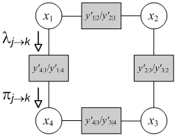
Figure 1: The ring-type pair-wise graph for 4ร—N4๐‘4\times N MIMO channel

II-B Low complexity detection based on BP over ring-type pair-wise graph [13]

Our start point is the one in [13], especially the BP over ring-type pair-wise graph. The graphical model is shown in Fig.1, over which the BP algorithm is effectively a forward-backward recursion and can be summarized as follows.

BP over ring-type pair-wise graph

Given the messages in the previous iteration, ฯ€(jโˆ“1)Mโ†’jโ€‹(xj)subscript๐œ‹โ†’subscriptminus-or-plus๐‘—1๐‘€๐‘—subscript๐‘ฅ๐‘—\pi_{(j\mp 1)_{M}\to j}(x_{j}), they are recursively updated for all j๐‘—j as

ฯ€jโ†’(jยฑ1)Msubscript๐œ‹โ†’๐‘—subscriptplus-or-minus๐‘—1๐‘€\displaystyle\pi_{j\to(j\pm 1)_{M}} (x(jยฑ1)M=s)subscript๐‘ฅsubscriptplus-or-minus๐‘—1๐‘€๐‘ \displaystyle(x_{(j\pm 1)_{M}}=s)
=\displaystyle= โˆ‘sโ€ฒโˆˆฮžฮณ(jยฑ1)M|jโ€‹(s|sโ€ฒ)โ‹…ฯ€(jโˆ“1)Mโ†’jโ€‹(xj=sโ€ฒ)subscriptsuperscript๐‘ โ€ฒฮžโ‹…subscript๐›พconditionalsubscriptplus-or-minus๐‘—1๐‘€๐‘—conditional๐‘ superscript๐‘ โ€ฒsubscript๐œ‹โ†’subscriptminus-or-plus๐‘—1๐‘€๐‘—subscript๐‘ฅ๐‘—superscript๐‘ โ€ฒ\displaystyle\sum_{s^{\prime}\in\Xi}{\gamma_{(j\pm 1)_{M}|j}(s|s^{\prime})\cdot\pi_{(j\mp 1)_{M}\to j}(x_{j}=s^{\prime})} (2)

with ฮณj|iโ€‹(s|sโ€ฒ)subscript๐›พconditional๐‘—๐‘–conditional๐‘ superscript๐‘ โ€ฒ\gamma_{j|{i}}(s|s^{\prime}) given by (9).
After a pre-defined number of iterations, the belief is finally obtained by

bโ€‹(xj)=ฯ€(j+1)Mโ†’jโ€‹(xj)โ‹…ฯ€(jโˆ’1)Mโ†’jโ€‹(xj).๐‘subscript๐‘ฅ๐‘—โ‹…subscript๐œ‹โ†’subscript๐‘—1๐‘€๐‘—subscript๐‘ฅ๐‘—subscript๐œ‹โ†’subscript๐‘—1๐‘€๐‘—subscript๐‘ฅ๐‘—\displaystyle b(x_{j})=\pi_{(j+1)_{M}\to j}(x_{j})\cdot\pi_{(j-1)_{M}\to j}(x_{j}). (3)

In (2) and (3), (โ‹…)Msubscriptโ‹…๐‘€(\cdot)_{M} is one-base modulo-M๐‘€M operation. Since using (โ‹…)Msubscriptโ‹…๐‘€(\cdot)_{M} is cumbersome, it will later be omitted.

In this algorithm, we used only factor to variable node message, ฯ€iโ†’jโ€‹(xj)subscript๐œ‹โ†’๐‘–๐‘—subscript๐‘ฅ๐‘—\pi_{i\to j}(x_{j}), since there is only two factor nodes connected to a variable node such that variable nodes simply pass the incoming message to the opposite side.

In (2), the translation function, ฮณj|jยฑ1โ€‹(s|sโ€ฒ)subscript๐›พconditional๐‘—plus-or-minus๐‘—1conditional๐‘ superscript๐‘ โ€ฒ\gamma_{j|{j\pm 1}}(s|s^{\prime}), (also known as branch metric in the context of forward-backward recursion along a trellis) is based on the conditional MMSE estimator of xjsubscript๐‘ฅ๐‘—x_{j} given xjยฑ1subscript๐‘ฅplus-or-minus๐‘—1x_{j\pm 1}. By defining the conditional estimator of xjsubscript๐‘ฅ๐‘—x_{j} given xisubscript๐‘ฅ๐‘–x_{i} as

๐’˜j|i=๐‘ฒ{j,i}โˆ’1โ€‹๐’‰jsubscript๐’˜conditional๐‘—๐‘–superscriptsubscript๐‘ฒ๐‘—๐‘–1subscript๐’‰๐‘—\displaystyle{\boldsymbol{w}}_{j|i}={\boldsymbol{K}}_{\{j,i\}}^{-1}{\boldsymbol{h}}_{j} (4)

and applying it to the received signal vector ๐’š๐’š{\boldsymbol{y}}, we have

yj|i=๐’˜j|iHโ€‹๐’š=aj|i,jโ€‹xj+aj|i,iโ€‹xi+nj|isubscript๐‘ฆconditional๐‘—๐‘–superscriptsubscript๐’˜conditional๐‘—๐‘–๐ป๐’šsubscript๐‘Žconditional๐‘—๐‘–๐‘—subscript๐‘ฅ๐‘—subscript๐‘Žconditional๐‘—๐‘–๐‘–subscript๐‘ฅ๐‘–subscript๐‘›conditional๐‘—๐‘–\displaystyle y_{j|i}={\boldsymbol{w}}_{j|i}^{H}{\boldsymbol{y}}=a_{j|i,j}x_{j}+a_{j|i,i}x_{i}+n_{j|i} (5)

where

๐‘ฒฮฆsubscript๐‘ฒฮฆ\displaystyle{\boldsymbol{K}}_{\Phi} =ฯƒ2โ€‹๐‘ฐ+โˆ‘kโˆ‰ฮฆ๐’‰kโ€‹๐’‰kHabsentsuperscript๐œŽ2๐‘ฐsubscript๐‘˜ฮฆsubscript๐’‰๐‘˜superscriptsubscript๐’‰๐‘˜๐ป\displaystyle=\sigma^{2}{\boldsymbol{I}}+\sum\nolimits_{k\notin\Phi}{{\boldsymbol{h}}_{k}{\boldsymbol{h}}_{k}^{H}} (6)
aj|i,ksubscript๐‘Žconditional๐‘—๐‘–๐‘˜\displaystyle a_{j|i,k} =๐’˜j|iHโ€‹๐’‰k=๐’‰jHโ€‹๐‘ฒ{j,i}โˆ’1โ€‹๐’‰kโ€‹forโ€‹k=iโ€‹orโ€‹jabsentsuperscriptsubscript๐’˜conditional๐‘—๐‘–๐ปsubscript๐’‰๐‘˜superscriptsubscript๐’‰๐‘—๐ปsuperscriptsubscript๐‘ฒ๐‘—๐‘–1subscript๐’‰๐‘˜for๐‘˜๐‘–or๐‘—\displaystyle={\boldsymbol{w}}_{j|i}^{H}{\boldsymbol{h}}_{k}={\boldsymbol{h}}_{j}^{H}{\boldsymbol{K}}_{\{j,i\}}^{-1}{\boldsymbol{h}}_{k}\hskip 8.0pt\textrm{for}\;k=i\;\textrm{or}\;j (7)
๐”ผโ€‹|nj|i|2๐”ผsuperscriptsubscript๐‘›conditional๐‘—๐‘–2\displaystyle\mathbb{E}|{n_{j|i}}{|^{2}} =๐’˜j|iHโ€‹๐‘ฒ{j,i}โ€‹๐’„j|i=๐’‰jHโ€‹๐‘ฒ{j,i}โˆ’1โ€‹๐’‰jโ‰กฯƒj|i2.absentsuperscriptsubscript๐’˜conditional๐‘—๐‘–๐ปsubscript๐‘ฒ๐‘—๐‘–subscript๐’„conditional๐‘—๐‘–superscriptsubscript๐’‰๐‘—๐ปsuperscriptsubscript๐‘ฒ๐‘—๐‘–1subscript๐’‰๐‘—superscriptsubscript๐œŽconditional๐‘—๐‘–2\displaystyle={\boldsymbol{w}}_{j|i}^{H}{{\boldsymbol{K}}_{\{j,i\}}}{\boldsymbol{c}}_{j|i}={\boldsymbol{h}}_{j}^{H}{\boldsymbol{K}}_{\{j,i\}}^{-1}{\boldsymbol{h}}_{j}\equiv\sigma_{j|i}^{2}. (8)

Note that ฯƒj|i2=aj|i,jsuperscriptsubscript๐œŽconditional๐‘—๐‘–2subscript๐‘Žconditional๐‘—๐‘–๐‘—\sigma_{j|i}^{2}=a_{j|i,j} and the parameters from (6) to (8) are computed from the channel parameters, ๐‘ฏ๐‘ฏ\boldsymbol{H} and ฯƒ2superscript๐œŽ2\sigma^{2}, and the received signal ๐’š๐’š\boldsymbol{y}. In the truncated signal model in (5), we assume the noise + interference, nj|isubscript๐‘›conditional๐‘—๐‘–n_{j|i}, to be a Gaussian, from which the translation function is given by

ฮณj|isubscript๐›พconditional๐‘—๐‘–\displaystyle\gamma_{{j}|i} (xj|xi)โˆ๐’žโ€‹๐’ฉโ€‹(yj|i;aj|i,jโ€‹xj+aj|i,iโ€‹xi,ฯƒj|i2)proportional-toconditionalsubscript๐‘ฅ๐‘—subscript๐‘ฅ๐‘–๐’ž๐’ฉsubscript๐‘ฆconditional๐‘—๐‘–subscript๐‘Žconditional๐‘—๐‘–๐‘—subscript๐‘ฅ๐‘—subscript๐‘Žconditional๐‘—๐‘–๐‘–subscript๐‘ฅ๐‘–superscriptsubscript๐œŽconditional๐‘—๐‘–2\displaystyle(x_{j}|x_{i})\propto\mathcal{CN}(y_{j|i};a_{j|i,j}x_{j}+a_{j|i,i}x_{i},\sigma_{j|i}^{2}) (9)

where ๐’žโ€‹๐’ฉโ€‹(x;a,b)๐’ž๐’ฉ๐‘ฅ๐‘Ž๐‘\mathcal{CN}(x;a,b) is the complex Gaussian density function with mean a๐‘Ža and variance b๐‘b given by

๐’žโ€‹๐’ฉโ€‹(y;ฮผ,ฯƒ2)๐’ž๐’ฉ๐‘ฆ๐œ‡superscript๐œŽ2\displaystyle\mathcal{CN}(y;\mu,\sigma^{2}) โ‰ก1ฯ€โ€‹ฯƒ2โ€‹expโก(โˆ’|yโˆ’ฮผ|2ฯƒ2)absent1๐œ‹superscript๐œŽ2superscript๐‘ฆ๐œ‡2superscript๐œŽ2\displaystyle\equiv\frac{1}{\pi\sigma^{2}}\exp\left(-\frac{|{y}-{\mu}|^{2}}{\sigma^{2}}\right)

The translation function given by Gaussian density function in (9) assumes data symbols other than xjsubscript๐‘ฅ๐‘—x_{j} and xisubscript๐‘ฅ๐‘–x_{i} are all Gaussian. This assumption, however, is only for pruning edges and to simplify the graphical model as shown in Fig.1 while the messages themselves in (2) are not necessarily Gaussian too.

On the other hand, when the input is indeed Gaussian, the forward backward algorithm in (2) reduces to an update rule for mean and variance [13] as follows.

Gaussian BP over ring-type pair-wise graph

Given the messages in the previous iteration, (ฮผฯ€,jโˆ“1โ†’j,ฯƒฯ€,jโˆ“1โ†’j2)subscript๐œ‡โ†’๐œ‹minus-or-plus๐‘—1๐‘—subscriptsuperscript๐œŽ2โ†’๐œ‹minus-or-plus๐‘—1๐‘—(\mu_{\pi,j\mp 1\rightarrow j},\sigma^{2}_{\pi,j\mp 1\rightarrow j}) โˆ€jfor-all๐‘—\forall j, they are recursively updat- ed by

ฯƒฯ€,jโ†’jยฑ12superscriptsubscript๐œŽโ†’๐œ‹๐‘—plus-or-minus๐‘—12\displaystyle\sigma_{\pi,j\to j\pm 1}^{2} =11+ฯƒjยฑ1|j2+|ajยฑ1|j,j|2(1+ฯƒjยฑ1|j2)2โ‹…ฯƒฯ€,jโˆ“1โ†’j2absent11superscriptsubscript๐œŽplus-or-minus๐‘—conditional1๐‘—2โ‹…superscriptsubscript๐‘Žplus-or-minus๐‘—conditional1๐‘—๐‘—2superscript1superscriptsubscript๐œŽplus-or-minus๐‘—conditional1๐‘—22superscriptsubscript๐œŽโ†’๐œ‹minus-or-plus๐‘—1๐‘—2\displaystyle=\frac{1}{{1+\sigma_{j\pm 1|j}^{2}}}+\frac{{|a_{j\pm 1|j,j}|^{2}}}{{(1+\sigma_{j\pm 1|j}^{2})^{2}}}\cdot\sigma_{\pi,j\mp 1\to j}^{2} (10)
ฮผฯ€,jโ†’jยฑ1subscript๐œ‡โ†’๐œ‹๐‘—plus-or-minus๐‘—1\displaystyle\mu_{\pi,j\to j\pm 1} =yjยฑ1|j1+ฯƒjยฑ1|j2โˆ’ajยฑ1|j,j1+ฯƒjยฑ1|j2โ‹…ฮผฯ€,jโˆ“1โ†’jabsentsubscript๐‘ฆplus-or-minus๐‘—conditional1๐‘—1superscriptsubscript๐œŽplus-or-minus๐‘—conditional1๐‘—2โ‹…subscript๐‘Žplus-or-minus๐‘—conditional1๐‘—๐‘—1superscriptsubscript๐œŽplus-or-minus๐‘—conditional1๐‘—2subscript๐œ‡โ†’๐œ‹minus-or-plus๐‘—1๐‘—\displaystyle=\frac{y_{j\pm 1|j}}{{1+\sigma_{j\pm 1|j}^{2}}}-\frac{{a_{j\pm 1|j,j}}}{{1+\sigma_{j\pm 1|j}^{2}}}\cdot\mu_{\pi,j\mp 1\to j} (11)

In [13], it is proved that the mean and variance in the Gaussian forward-backward recursion converge respectively to MMSE estimates and its corresponding MMSE, i.e.,

ฮผฯ€,jโˆ“1โ†’jโ†’โ†’subscript๐œ‡โ†’๐œ‹minus-or-plus๐‘—1๐‘—absent\displaystyle\mu_{\pi,j\mp 1\to j}\rightarrow x^j=๐’‰jHโ€‹๐‘ฒโˆ’1โ€‹๐’šsubscript^๐‘ฅ๐‘—superscriptsubscript๐’‰๐‘—๐ปsuperscript๐‘ฒ1๐’š\displaystyle\;\hat{x}_{j}={\boldsymbol{h}}_{j}^{H}{\boldsymbol{K}}^{-1}{\boldsymbol{y}} (12)
ฯƒฯ€,jโˆ“1โ†’j2โ†’โ†’subscriptsuperscript๐œŽ2โ†’๐œ‹minus-or-plus๐‘—1๐‘—absent\displaystyle\sigma^{2}_{\pi,j\mp 1\rightarrow j}\rightarrow MMSEj=1โˆ’๐’‰jHโ€‹๐‘ฒโˆ’1โ€‹๐’‰j.subscriptMMSE๐‘—1superscriptsubscript๐’‰๐‘—๐ปsuperscript๐‘ฒ1subscript๐’‰๐‘—\displaystyle\;\text{MMSE}_{j}=1-{\boldsymbol{h}}_{j}^{H}{\boldsymbol{K}}^{-1}{\boldsymbol{h}}_{j}. (13)

as the number of iteration goes to infinity. Since MAP detector becomes linear MMSE estimator for the Gaussian input, it shows the optimality of the scheme for Gaussian input. However, for the non-Gaussian input, MMSE estimator is far inferior to MAP detector.

In the rest of this paper, we deal with the convergence of the forward-backward algorithm in (2) for arbitrary discrete alphabet and its density evolution characteristic for binary input, which will give us a deeper insight into its convergence and performance.

III Convergence for Discrete Alphabet

In this section, we provide two convergence proofs of the BP over ring-type pair-wise graph, one for arbitrary discrete alphabet and the other for binary one. The signal model for binary input provides framework not only for the convergence proof but also for density evolution analysis to be discussed in the next section.

III-A Convergence proof for arbitrary discrete input

The convergence proof in this subsection is based on the โ€™Perron-Frobenius theoremโ€™. Although it has already been discussed in [21], we provide it in our context here for the readerโ€™s convenience.

Suppose that data symbols are drawn from an 2msuperscript2๐‘š2^{m}-ary alphabet set ฮž={s1,s2,โ€ฆ,s2m}ฮžsubscript๐‘ 1subscript๐‘ 2โ€ฆsubscript๐‘ superscript2๐‘š\Xi=\{s_{1},s_{2},...,s_{2^{m}}\}. The forward-backward recursion in (2) can be concisely expressed as

๐…jโ†’jยฑ1subscript๐…โ†’๐‘—plus-or-minus๐‘—1\displaystyle{\boldsymbol{\pi}}_{j\to j\pm 1} =1ฮฑjยฑ1โ€‹๐‘จjยฑ1|jโ€‹๐…jโˆ“1โ†’jabsent1subscript๐›ผplus-or-minus๐‘—1subscript๐‘จplus-or-minus๐‘—conditional1๐‘—subscript๐…โ†’minus-or-plus๐‘—1๐‘—\displaystyle=\frac{1}{\alpha_{j\pm 1}}{\boldsymbol{A}}_{j\pm 1|j}{\boldsymbol{\pi}}_{j\mp 1\to j} (14)

where ๐…iโ†’jsubscript๐…โ†’๐‘–๐‘—{\boldsymbol{\pi}}_{i\to j} is Mร—1๐‘€1M\times 1 message vector of which the m๐‘šmth element is given by ฯ€iโ†’jโ€‹(xj=sm)subscript๐œ‹โ†’๐‘–๐‘—subscript๐‘ฅ๐‘—subscript๐‘ ๐‘š{\pi}_{i\to j}(x_{j}=s_{m}), ๐‘จj|isubscript๐‘จconditional๐‘—๐‘–{\boldsymbol{A}}_{j|i} is Mร—M๐‘€๐‘€M\times M translation matrix of which the (m,n๐‘š๐‘›m,n)th element is ฮณj|iโ€‹(xj=sm|xi=sn)subscript๐›พconditional๐‘—๐‘–subscript๐‘ฅ๐‘—conditionalsubscript๐‘ ๐‘šsubscript๐‘ฅ๐‘–subscript๐‘ ๐‘›\gamma_{j|i}(x_{j}=s_{m}|x_{i}=s_{n}) and ฮฑjsubscript๐›ผ๐‘—\alpha_{j} is the normalization constant, such that โ€–๐…iโ†’jโ€–1=1subscriptnormsubscript๐…โ†’๐‘–๐‘—11\|{\boldsymbol{\pi}}_{i\to j}\|_{1}=1, i.e., ฮฑj=โ€–๐‘จj|iโ€‹๐…iโ†’jโ€–1subscript๐›ผ๐‘—subscriptnormsubscript๐‘จconditional๐‘—๐‘–subscript๐…โ†’๐‘–๐‘—1\alpha_{j}=\|{\boldsymbol{A}}_{j|i}{\boldsymbol{\pi}}_{i\to j}\|_{1}.111โ€–๐’‚โ€–1subscriptnorm๐’‚1\|{\boldsymbol{a}}\|_{1} denotes the L1subscript๐ฟ1L_{1}-norm of a vector ๐’‚๐’‚{\boldsymbol{a}} Note that all element of ๐‘จj|isubscript๐‘จconditional๐‘—๐‘–{\boldsymbol{A}}_{j|i} are positive real.

Define ๐‘ญjsubscript๐‘ญ๐‘—{\boldsymbol{F}}_{j} and ๐‘ฉjsubscript๐‘ฉ๐‘—{\boldsymbol{B}}_{j} as the translation matrix for one complete turn of forward and backward recursion, respectively, i.e.,

๐‘ญjsubscript๐‘ญ๐‘—\displaystyle{\boldsymbol{F}}_{j} =๐‘จj|jโˆ’1โ€‹๐‘จjโˆ’1|jโˆ’2โ€‹โ‹ฏโ€‹๐‘จ2|1โ€‹๐‘จ1|Mโ€‹โ‹ฏโ€‹๐‘จj+1|jabsentsubscript๐‘จconditional๐‘—๐‘—1subscript๐‘จ๐‘—conditional1๐‘—2โ‹ฏsubscript๐‘จconditional21subscript๐‘จconditional1๐‘€โ‹ฏsubscript๐‘จ๐‘—conditional1๐‘—\displaystyle={\boldsymbol{A}}_{j|j-1}{\boldsymbol{A}}_{j-1|j-2}\cdots{\boldsymbol{A}}_{2|1}{\boldsymbol{A}}_{1|M}\cdots{\boldsymbol{A}}_{j+1|j} (15)
๐‘ฉjsubscript๐‘ฉ๐‘—\displaystyle{\boldsymbol{B}}_{j} =๐‘จj|j+1โ€‹๐‘จj+1|j+2โ€‹โ‹ฏโ€‹๐‘จMโˆ’1|Mโ€‹๐‘จM|1โ€‹โ‹ฏโ€‹๐‘จjโˆ’1|jabsentsubscript๐‘จconditional๐‘—๐‘—1subscript๐‘จ๐‘—conditional1๐‘—2โ‹ฏsubscript๐‘จ๐‘€conditional1๐‘€subscript๐‘จconditional๐‘€1โ‹ฏsubscript๐‘จ๐‘—conditional1๐‘—\displaystyle={\boldsymbol{A}}_{j|j+1}{\boldsymbol{A}}_{j+1|j+2}\cdots{\boldsymbol{A}}_{M-1|M}{\boldsymbol{A}}_{M|1}\cdots{\boldsymbol{A}}_{j-1|j} (16)

Then, the message vector at the k๐‘˜kth turn can be expressed as

๐…jโˆ’1โ†’j(k)โˆ๐‘ญjโ€‹๐…jโˆ’1โ†’j(kโˆ’1)=๐‘ญjkโ€‹๐…0proportional-tosuperscriptsubscript๐…โ†’๐‘—1๐‘—๐‘˜subscript๐‘ญ๐‘—superscriptsubscript๐…โ†’๐‘—1๐‘—๐‘˜1superscriptsubscript๐‘ญ๐‘—๐‘˜subscript๐…0\displaystyle{\boldsymbol{\pi}}_{j-1\to j}^{(k)}\propto{\boldsymbol{F}}_{j}{\boldsymbol{\pi}}_{j-1\to j}^{(k-1)}={\boldsymbol{F}}_{j}^{k}{\boldsymbol{\pi}}_{0} (17)
๐…j+1โ†’j(k)โˆ๐‘ฉjโ€‹๐…j+1โ†’j(kโˆ’1)=๐‘ฉjkโ€‹๐…0proportional-tosuperscriptsubscript๐…โ†’๐‘—1๐‘—๐‘˜subscript๐‘ฉ๐‘—superscriptsubscript๐…โ†’๐‘—1๐‘—๐‘˜1superscriptsubscript๐‘ฉ๐‘—๐‘˜subscript๐…0\displaystyle{\boldsymbol{\pi}}_{j+1\to j}^{(k)}\propto{\boldsymbol{B}}_{j}{\boldsymbol{\pi}}_{j+1\to j}^{(k-1)}={\boldsymbol{B}}_{j}^{k}{\boldsymbol{\pi}}_{0} (18)

where ๐…jยฑ1โ†’j(k)superscriptsubscript๐…โ†’plus-or-minus๐‘—1๐‘—๐‘˜{\boldsymbol{\pi}}_{j\pm 1\to j}^{(k)} is the message at the k๐‘˜kth turn and ๐…0subscript๐…0{\boldsymbol{\pi}}_{0} is the initial message, which is typically set to uniform distribution. Now, one can prove the following theorem.

Theorem 1

With any initial message, ๐›‘0subscript๐›‘0{\boldsymbol{\pi}}_{0}, the message ๐›‘jโˆ’1โ†’j(k)superscriptsubscript๐›‘โ†’๐‘—1๐‘—๐‘˜{\boldsymbol{\pi}}_{j-1\to j}^{(k)} in (17) converges (up to a normalization constant) to the eigenvector of ๐…jsubscript๐…๐‘—{\boldsymbol{F}}_{j} corresponding to its largest eigenvalue. Similarly, ๐›‘j+1โ†’j(k)superscriptsubscript๐›‘โ†’๐‘—1๐‘—๐‘˜{\boldsymbol{\pi}}_{j+1\to j}^{(k)} in (18) converges to the eigenvector of ๐jsubscript๐๐‘—{\boldsymbol{B}}_{j} corresponding to its largest eigenvalue.

Proof:

First, we decomposed the transition matrix for one complete turn, ๐‘ญjsubscript๐‘ญ๐‘—{\boldsymbol{F}}_{j}, into

๐‘ญjsubscript๐‘ญ๐‘—\displaystyle{\boldsymbol{F}}_{j} =๐‘ฌjโ€‹๐‘ซjโ€‹๐‘ฌjโˆ’1absentsubscript๐‘ฌ๐‘—subscript๐‘ซ๐‘—superscriptsubscript๐‘ฌ๐‘—1\displaystyle={\boldsymbol{E}}_{j}{\boldsymbol{D}}_{j}{\boldsymbol{E}}_{j}^{-1}

where ๐‘ซjsubscript๐‘ซ๐‘—{\boldsymbol{D}}_{j} is diagonal matrix with its m๐‘šmth diagonal element is the m๐‘šmth eigenvalue, ฮปmsubscript๐œ†๐‘š\lambda_{m}, and ๐‘ฌjsubscript๐‘ฌ๐‘—{\boldsymbol{E}}_{j} is the eigenbasis, of which the m๐‘šmth column, ๐’†msubscript๐’†๐‘š{\boldsymbol{e}}_{m}, is the eigenvector for ฮปmsubscript๐œ†๐‘š\lambda_{m}. Then, we have

๐‘ญjksuperscriptsubscript๐‘ญ๐‘—๐‘˜\displaystyle{\boldsymbol{F}}_{j}^{k} =๐‘ฌjโ€‹๐‘ซjkโ€‹๐‘ฌjโˆ’1absentsubscript๐‘ฌ๐‘—superscriptsubscript๐‘ซ๐‘—๐‘˜superscriptsubscript๐‘ฌ๐‘—1\displaystyle={\boldsymbol{E}}_{j}{\boldsymbol{D}}_{j}^{k}{\boldsymbol{E}}_{j}^{-1}
=[ฮป1kโ€‹๐’†1โ€‹ฮป2kโ€‹๐’†2โ€‹โ‹ฏโ€‹ฮปMkโ€‹๐’†M]โ‹…[i11i12โ‹ฏi1โ€‹Mi21i22i2โ€‹Mโ‹ฎโ‹ฑโ‹ฎiMโ€‹1iMโ€‹2โ‹ฏiMโ€‹M]absentโ‹…delimited-[]superscriptsubscript๐œ†1๐‘˜subscript๐’†1superscriptsubscript๐œ†2๐‘˜subscript๐’†2โ‹ฏsuperscriptsubscript๐œ†๐‘€๐‘˜subscript๐’†๐‘€matrixsubscript๐‘–11subscript๐‘–12โ‹ฏsubscript๐‘–1๐‘€subscript๐‘–21subscript๐‘–22missing-subexpressionsubscript๐‘–2๐‘€โ‹ฎmissing-subexpressionโ‹ฑโ‹ฎsubscript๐‘–๐‘€1subscript๐‘–๐‘€2โ‹ฏsubscript๐‘–๐‘€๐‘€\displaystyle=\left[\lambda_{1}^{k}{\boldsymbol{e}}_{1}\lambda_{2}^{k}{\boldsymbol{e}}_{2}\cdots\lambda_{M}^{k}{\boldsymbol{e}}_{M}\right]\cdot\begin{bmatrix}i_{11}&i_{12}&\cdots&i_{1M}\\ i_{21}&i_{22}&&i_{2M}\\ \vdots&&\ddots&\vdots\\ i_{M1}&i_{M2}&\cdots&i_{MM}\\ \end{bmatrix}

where imโ€‹nsubscript๐‘–๐‘š๐‘›i_{mn} is the (m,n๐‘š๐‘›m,n)th element of ๐‘ฌjโˆ’1superscriptsubscript๐‘ฌ๐‘—1{\boldsymbol{E}}_{j}^{-1}. Note that, with an initial message, ๐…0subscript๐…0{\boldsymbol{\pi}}_{0}, we have

[๐…jโˆ’1โ†’j(k)]msubscriptdelimited-[]subscriptsuperscript๐…๐‘˜โ†’๐‘—1๐‘—๐‘š\displaystyle\left[{\boldsymbol{\pi}}^{(k)}_{j-1\to j}\right]_{m} =[๐‘ญjkโ€‹๐…0]m=โˆ‘n=1Mโˆ‘l=1Memโ€‹lโ€‹ฮปlkโ€‹ilโ€‹nโ€‹ฯ€0,nabsentsubscriptdelimited-[]superscriptsubscript๐‘ญ๐‘—๐‘˜subscript๐…0๐‘šsuperscriptsubscript๐‘›1๐‘€superscriptsubscript๐‘™1๐‘€subscript๐‘’๐‘š๐‘™superscriptsubscript๐œ†๐‘™๐‘˜subscript๐‘–๐‘™๐‘›subscript๐œ‹0๐‘›\displaystyle=\left[{\boldsymbol{F}}_{j}^{k}{\boldsymbol{\pi}}_{0}\right]_{m}=\sum_{n=1}^{M}\sum_{l=1}^{M}e_{ml}\lambda_{l}^{k}i_{ln}\pi_{0,n} (19)

Since all the entries of ๐‘ญjksuperscriptsubscript๐‘ญ๐‘—๐‘˜{\boldsymbol{F}}_{j}^{k} are positive, we see, from Perron-Frobenius theorem, that the matrix, ๐‘ญjsubscript๐‘ญ๐‘—{\boldsymbol{F}}_{j}, has single largest real eigenvalue (a.k.a. Perron-Frobenius eigenvalue) of which the corresponding eigenvector has (or can be chosen to have) all positive entries. Let ฮปlโˆ—subscript๐œ†superscript๐‘™{\lambda}_{l^{*}} be the largest real eigenvalue and ๐’†lโˆ—subscript๐’†superscript๐‘™{\boldsymbol{e}}_{l^{*}} the corresponding eigenvector. Then, by taking limit kโ†’โˆžโ†’๐‘˜k\to\infty to the normalized message [๐…jโˆ’1โ†’j(k)]msubscriptdelimited-[]subscriptsuperscript๐…๐‘˜โ†’๐‘—1๐‘—๐‘š[{\boldsymbol{\pi}}^{(k)}_{j-1\to j}]_{m} /โ€–๐…jโˆ’1โ†’j(k)โ€–1absentsubscriptnormsuperscriptsubscript๐…โ†’๐‘—1๐‘—๐‘˜1/\|{\boldsymbol{\pi}}_{j-1\to j}^{(k)}\|_{1}, we have

limkโ†’โˆž[๐…jโˆ’1โ†’j(k)]mโ€–๐…jโˆ’1โ†’j(k)โ€–1subscriptโ†’๐‘˜subscriptdelimited-[]subscriptsuperscript๐…๐‘˜โ†’๐‘—1๐‘—๐‘šsubscriptnormsuperscriptsubscript๐…โ†’๐‘—1๐‘—๐‘˜1\displaystyle\lim_{k\to\infty}\frac{[{\boldsymbol{\pi}}^{(k)}_{j-1\to j}]_{m}}{\|{\boldsymbol{\pi}}_{j-1\to j}^{(k)}\|_{1}} โ†’โˆ‘n=1Memโ€‹lโˆ—โ€‹ฮปlโˆ—kโ€‹ilโˆ—โ€‹nโ€‹ฯ€0,nโˆ‘mโ€ฒ=1Mโˆ‘n=1Memโ€ฒโ€‹lโˆ—โ€‹ฮปlโˆ—kโ€‹ilโˆ—โ€‹nโ€‹ฯ€0,nโ†’absentsuperscriptsubscript๐‘›1๐‘€subscript๐‘’๐‘šsuperscript๐‘™superscriptsubscript๐œ†superscript๐‘™๐‘˜subscript๐‘–superscript๐‘™๐‘›subscript๐œ‹0๐‘›superscriptsubscriptsuperscript๐‘šโ€ฒ1๐‘€superscriptsubscript๐‘›1๐‘€subscript๐‘’superscript๐‘šโ€ฒsuperscript๐‘™superscriptsubscript๐œ†superscript๐‘™๐‘˜subscript๐‘–superscript๐‘™๐‘›subscript๐œ‹0๐‘›\displaystyle\to\frac{\sum_{n=1}^{M}e_{ml^{*}}\lambda_{l^{*}}^{k}i_{{l^{*}}n}\pi_{0,n}}{\sum_{m^{\prime}=1}^{M}\sum_{n=1}^{M}e_{m^{\prime}l^{*}}\lambda_{l^{*}}^{k}i_{{l^{*}}n}\pi_{0,n}}
=emโ€‹lโˆ—โ€‹ฮปlโˆ—kโ€‹โˆ‘n=1Milโˆ—โ€‹nโ€‹ฯ€0,nโˆ‘mโ€ฒ=1Memโ€ฒโ€‹lโˆ—โ€‹ฮปlโˆ—kโ€‹โˆ‘n=1Milโˆ—โ€‹nโ€‹ฯ€0,nabsentsubscript๐‘’๐‘šsuperscript๐‘™superscriptsubscript๐œ†superscript๐‘™๐‘˜superscriptsubscript๐‘›1๐‘€subscript๐‘–superscript๐‘™๐‘›subscript๐œ‹0๐‘›superscriptsubscriptsuperscript๐‘šโ€ฒ1๐‘€subscript๐‘’superscript๐‘šโ€ฒsuperscript๐‘™superscriptsubscript๐œ†superscript๐‘™๐‘˜superscriptsubscript๐‘›1๐‘€subscript๐‘–superscript๐‘™๐‘›subscript๐œ‹0๐‘›\displaystyle=\frac{e_{ml^{*}}\lambda_{l^{*}}^{k}\sum_{n=1}^{M}i_{{l^{*}}n}\pi_{0,n}}{\sum_{m^{\prime}=1}^{M}e_{m^{\prime}l^{*}}\lambda_{l^{*}}^{k}\sum_{n=1}^{M}i_{{l^{*}}n}\pi_{0,n}}
=emโ€‹lโˆ—โˆ‘mโ€ฒ=1Memโ€ฒโ€‹lโˆ—absentsubscript๐‘’๐‘šsuperscript๐‘™superscriptsubscriptsuperscript๐‘šโ€ฒ1๐‘€subscript๐‘’superscript๐‘šโ€ฒsuperscript๐‘™\displaystyle=\frac{e_{ml^{*}}}{\sum_{m^{\prime}=1}^{M}e_{m^{\prime}l^{*}}}
=[๐’†lโˆ—]mโ€–๐’†lโˆ—โ€–1absentsubscriptdelimited-[]subscript๐’†superscript๐‘™๐‘šsubscriptnormsubscript๐’†superscript๐‘™1\displaystyle=\frac{[{\boldsymbol{e}}_{l^{*}}]_{m}}{\|{\boldsymbol{e}}_{l^{*}}\|_{1}} (20)

where, in the r.h.s. of the first line, we took only the term with the largest eigenvalue since other terms are negligible as kโ†’โˆžโ†’๐‘˜k\to\infty.

The convergence for the backward recursion can be proved similarly. โˆŽ

Although the convergence proof below is applicable to arbitrary alphabet, it is not suitable for further SINR and BER analysis. So, we provides another signal model which deals directly with the log-likelihood ratio (LLR) by restricting the data to binary. As will be shown later, it gives us a more convenient way for SINR and BER analysis via density evolution.

III-B Message passing for binary input

For binary input, the message can be summarized by a scalar, i.e., the log likelihood ratio(LLR). Define the message and a priori LLR as

liโ†’jsubscript๐‘™โ†’๐‘–๐‘—\displaystyle l_{i\rightarrow j} =logโกฯ€iโ†’jโ€‹(xj=+1)ฯ€iโ†’jโ€‹(xj=โˆ’1)absentsubscript๐œ‹โ†’๐‘–๐‘—subscript๐‘ฅ๐‘—1subscript๐œ‹โ†’๐‘–๐‘—subscript๐‘ฅ๐‘—1\displaystyle=\log\frac{\pi_{i\rightarrow j}(x_{j}=+1)}{\pi_{i\rightarrow j}(x_{j}=-1)} (21)
la,isubscript๐‘™๐‘Ž๐‘–\displaystyle l_{a,i} =logโกpโ€‹(xi=+1)pโ€‹(xi=โˆ’1)absent๐‘subscript๐‘ฅ๐‘–1๐‘subscript๐‘ฅ๐‘–1\displaystyle=\log\frac{p(x_{i}=+1)}{p(x_{i}=-1)} (22)

such that

pโ€‹(xi=ยฑ1)๐‘subscript๐‘ฅ๐‘–plus-or-minus1\displaystyle p(x_{i}=\pm 1) =eยฑla,i/2e+la,i/2+eโˆ’la,i/2absentsuperscript๐‘’plus-or-minussubscript๐‘™๐‘Ž๐‘–2superscript๐‘’subscript๐‘™๐‘Ž๐‘–2superscript๐‘’subscript๐‘™๐‘Ž๐‘–2\displaystyle=\frac{e^{\pm l_{a,i}/2}}{e^{+l_{a,i}/2}+e^{-l_{a,i}/2}}

Then, the forward recursion in (2), together with (21), can be expressed as (23) shown on top of the next page, where we assume uniform priors.

liโ†’jsubscript๐‘™โ†’๐‘–๐‘—\displaystyle l_{i\rightarrow j} =logโก(pโ€‹(xj=+1)โ€‹โˆ‘xjโˆ’1=ยฑ1๐’žโ€‹๐’ฉโ€‹(yj|jโˆ’1โ€ฒ;+aj|jโˆ’1,j+aj|jโˆ’1,jโˆ’1โ€‹xjโˆ’1,ฯƒj|jโˆ’12)โ€‹ฯ€jโˆ’2โ†’jโˆ’1โ€‹(xjโˆ’1)pโ€‹(xj=โˆ’1)โ€‹โˆ‘xjโˆ’1=ยฑ1๐’žโ€‹๐’ฉโ€‹(yj|jโˆ’1โ€ฒ;โˆ’aj|jโˆ’1,j+aj|jโˆ’1,jโˆ’1โ€‹xjโˆ’1,ฯƒj|jโˆ’12)โ€‹ฯ€jโˆ’2โ†’jโˆ’1โ€‹(xjโˆ’1))absent๐‘subscript๐‘ฅ๐‘—1subscriptsubscript๐‘ฅ๐‘—1plus-or-minus1๐’ž๐’ฉsubscriptsuperscript๐‘ฆโ€ฒconditional๐‘—๐‘—1subscript๐‘Žconditional๐‘—๐‘—1๐‘—subscript๐‘Žconditional๐‘—๐‘—1๐‘—1subscript๐‘ฅ๐‘—1superscriptsubscript๐œŽconditional๐‘—๐‘—12subscript๐œ‹โ†’๐‘—2๐‘—1subscript๐‘ฅ๐‘—1๐‘subscript๐‘ฅ๐‘—1subscriptsubscript๐‘ฅ๐‘—1plus-or-minus1๐’ž๐’ฉsubscriptsuperscript๐‘ฆโ€ฒconditional๐‘—๐‘—1subscript๐‘Žconditional๐‘—๐‘—1๐‘—subscript๐‘Žconditional๐‘—๐‘—1๐‘—1subscript๐‘ฅ๐‘—1superscriptsubscript๐œŽconditional๐‘—๐‘—12subscript๐œ‹โ†’๐‘—2๐‘—1subscript๐‘ฅ๐‘—1\displaystyle=\log\left(\frac{p(x_{j}=+1)\displaystyle\sum_{x_{j-1}=\pm 1}\mathcal{CN}(y^{\prime}_{j|j-1};+a_{j|j-1,j}+a_{j|j-1,j-1}x_{j-1},\sigma_{j|j-1}^{2})\pi_{j-2\to j-1}(x_{j-1})}{p(x_{j}=-1)\displaystyle\sum_{x_{j-1}=\pm 1}\mathcal{CN}(y^{\prime}_{j|j-1};-a_{j|j-1,j}+a_{j|j-1,j-1}x_{j-1},\sigma_{j|j-1}^{2})\pi_{j-2\to j-1}(x_{j-1})}\right)
=la,j+logโก(โˆ‘xjโˆ’1=ยฑ1expโก(โˆ’|yj|jโˆ’1โˆ’aj|jโˆ’1,jโˆ’aj|jโˆ’1,jโˆ’1โ€‹xjโˆ’1|2ฯƒj|jโˆ’12+ljโˆ’2โ†’jโˆ’1โ€‹xjโˆ’12)โˆ‘xjโˆ’1=ยฑ1expโก(โˆ’|yj|jโˆ’1+aj|jโˆ’1,jโˆ’aj|jโˆ’1,jโˆ’1โ€‹xjโˆ’1|2ฯƒj|jโˆ’12+ljโˆ’2โ†’jโˆ’1โ€‹xjโˆ’12))absentsubscript๐‘™๐‘Ž๐‘—subscriptsubscript๐‘ฅ๐‘—1plus-or-minus1superscriptsubscript๐‘ฆconditional๐‘—๐‘—1subscript๐‘Žconditional๐‘—๐‘—1๐‘—subscript๐‘Žconditional๐‘—๐‘—1๐‘—1subscript๐‘ฅ๐‘—12subscriptsuperscript๐œŽ2conditional๐‘—๐‘—1subscript๐‘™โ†’๐‘—2๐‘—1subscript๐‘ฅ๐‘—12subscriptsubscript๐‘ฅ๐‘—1plus-or-minus1superscriptsubscript๐‘ฆconditional๐‘—๐‘—1subscript๐‘Žconditional๐‘—๐‘—1๐‘—subscript๐‘Žconditional๐‘—๐‘—1๐‘—1subscript๐‘ฅ๐‘—12subscriptsuperscript๐œŽ2conditional๐‘—๐‘—1subscript๐‘™โ†’๐‘—2๐‘—1subscript๐‘ฅ๐‘—12\displaystyle=l_{a,j}+\log\left(\frac{\displaystyle\sum_{x_{j-1}=\pm 1}\exp\left(-\frac{|y_{j|j-1}-a_{j|j-1,j}-a_{j|j-1,j-1}x_{j-1}|^{2}}{\sigma^{2}_{j|j-1}}+\frac{l_{j-2\rightarrow j-1}x_{j-1}}{2}\right)}{\displaystyle\sum_{x_{j-1}=\pm 1}\exp\left(-\frac{|y_{j|j-1}+a_{j|j-1,j}-a_{j|j-1,j-1}x_{j-1}|^{2}}{\sigma^{2}_{j|j-1}}+\frac{l_{j-2\rightarrow j-1}x_{j-1}}{2}\right)}\right) (23)

Removing common terms in the numerator and denominator in (23) and defining a function ฮถโ€‹(x;c)๐œ๐‘ฅ๐‘\zeta(x;c) of x๐‘ฅx with a parameter c๐‘c as

ฮถโ€‹(x;c)=โˆ’logโก(ex/2โˆ’c+eโˆ’x/2+cex/2+c+eโˆ’x/2โˆ’c)๐œ๐‘ฅ๐‘superscript๐‘’๐‘ฅ2๐‘superscript๐‘’๐‘ฅ2๐‘superscript๐‘’๐‘ฅ2๐‘superscript๐‘’๐‘ฅ2๐‘\displaystyle\zeta(x;c)=-\log\left(\frac{e^{x/2-c}+e^{-x/2+c}}{e^{x/2+c}+e^{-x/2-c}}\right) (24)

(23) can be concisely rewritten as

ljโˆ’1โ†’j=la,j+4โ€‹yj|jโˆ’1(R)โˆ’ฮถโ€‹(ljโˆ’2โ†’jโˆ’1+2โ€‹dj|jโˆ’1;cj|jโˆ’1)subscript๐‘™โ†’๐‘—1๐‘—subscript๐‘™๐‘Ž๐‘—4subscriptsuperscript๐‘ฆ๐‘…conditional๐‘—๐‘—1๐œsubscript๐‘™โ†’๐‘—2๐‘—12subscript๐‘‘conditional๐‘—๐‘—1subscript๐‘conditional๐‘—๐‘—1\displaystyle l_{j-1\to j}=l_{a,j}+4y^{(R)}_{j|j-1}-\zeta(l_{j-2\to j-1}+2d_{j|j-1};c_{j|j-1}) (25)

where

yj|i(R)subscriptsuperscript๐‘ฆ๐‘…conditional๐‘—๐‘–\displaystyle y^{(R)}_{j|i} =โ„œโก[yj|i]absentsubscript๐‘ฆconditional๐‘—๐‘–\displaystyle=\Re[y_{j|i}] (26)
cj|isubscript๐‘conditional๐‘—๐‘–\displaystyle c_{j|i} =2ฯƒj|i2โ€‹โ„œโก[aj|i,jโˆ—โ€‹aj|i,i]=2โ€‹โ„œโก[aj|i,i]=2โ€‹aj|i,i(R)absent2subscriptsuperscript๐œŽ2conditional๐‘—๐‘–subscriptsuperscript๐‘Žconditional๐‘—๐‘–๐‘—subscript๐‘Žconditional๐‘—๐‘–๐‘–2subscript๐‘Žconditional๐‘—๐‘–๐‘–2subscriptsuperscript๐‘Ž๐‘…conditional๐‘—๐‘–๐‘–\displaystyle=\frac{2}{\sigma^{2}_{j|i}}\Re[a^{*}_{j|i,j}a_{j|i,i}]=2\Re[a_{j|i,i}]=2a^{(R)}_{j|i,i} (27)
dj|isubscript๐‘‘conditional๐‘—๐‘–\displaystyle d_{j|i} =2ฯƒj|i2โ€‹โ„œโก[aj|i,iโˆ—โ€‹yj|i]absent2subscriptsuperscript๐œŽ2conditional๐‘—๐‘–subscriptsuperscript๐‘Žconditional๐‘—๐‘–๐‘–subscript๐‘ฆconditional๐‘—๐‘–\displaystyle=\frac{2}{\sigma^{2}_{j|i}}\Re[a^{*}_{j|i,i}y_{j|i}]
=2โ€‹โ„œโก[aj|i,iโˆ—]โ€‹xj+2โ€‹|aj|i,i|2ฯƒj|i2โ€‹xi+2ฯƒj|i2โ€‹โ„œโก[aj|i,jโˆ—โ€‹nj|i]absent2subscriptsuperscript๐‘Žconditional๐‘—๐‘–๐‘–subscript๐‘ฅ๐‘—2superscriptsubscript๐‘Žconditional๐‘—๐‘–๐‘–2subscriptsuperscript๐œŽ2conditional๐‘—๐‘–subscript๐‘ฅ๐‘–2subscriptsuperscript๐œŽ2conditional๐‘—๐‘–subscriptsuperscript๐‘Žconditional๐‘—๐‘–๐‘—subscript๐‘›conditional๐‘—๐‘–\displaystyle=2\Re[a^{*}_{j|i,i}]x_{j}+\frac{2|a_{j|i,i}|^{2}}{\sigma^{2}_{j|i}}x_{i}+\frac{2}{\sigma^{2}_{j|i}}\Re[a^{*}_{j|i,j}n_{j|i}]
=2โ€‹aj|i,i(R)โ€‹xj+2โ€‹|aj|i,i|2ฯƒj|i2โ€‹xiabsent2subscriptsuperscript๐‘Ž๐‘…conditional๐‘—๐‘–๐‘–subscript๐‘ฅ๐‘—2superscriptsubscript๐‘Žconditional๐‘—๐‘–๐‘–2subscriptsuperscript๐œŽ2conditional๐‘—๐‘–subscript๐‘ฅ๐‘–\displaystyle=2a^{(R)}_{j|i,i}x_{j}+\frac{2|a_{j|i,i}|^{2}}{\sigma^{2}_{j|i}}x_{i}
+2ฯƒj|i2โ€‹(aj|i,j(R)โ€‹nj|i(R)+aj|i,j(I)โ€‹nj|i(I))2subscriptsuperscript๐œŽ2conditional๐‘—๐‘–subscriptsuperscript๐‘Ž๐‘…conditional๐‘—๐‘–๐‘—subscriptsuperscript๐‘›๐‘…conditional๐‘—๐‘–subscriptsuperscript๐‘Ž๐ผconditional๐‘—๐‘–๐‘—subscriptsuperscript๐‘›๐ผconditional๐‘—๐‘–\displaystyle\;\;\;\;+\frac{2}{\sigma^{2}_{j|i}}\left(a^{(R)}_{j|i,j}n^{(R)}_{j|i}+a^{(I)}_{j|i,j}n^{(I)}_{j|i}\right) (28)

where we denote the real and imaginary part of a complex variable as superscript (R๐‘…R) and (I๐ผI), respectively, for notational simplicity.

The non-linear function ฮถโ€‹(x;c)๐œ๐‘ฅ๐‘\zeta(x;c) in (24) is a monotonic function of x๐‘ฅx, either increasing if c>0๐‘0c>0 or decreasing if c<0๐‘0c<0, and has the following properties.

(a)โ€‹ฮถโ€ฒโ€‹(x;c)=ddโ€‹xโ€‹ฮถโ€‹(x;c)๐‘Žsuperscript๐œโ€ฒ๐‘ฅ๐‘dd๐‘ฅ๐œ๐‘ฅ๐‘\displaystyle(a)\;\;\zeta^{\prime}(x;c)=\frac{\mathrm{d}}{\mathrm{d}x}\zeta(x;c)
=12โ€‹tanhโก(x2+c)โˆ’12โ€‹tanhโก(x2โˆ’c)absent12๐‘ฅ2๐‘12๐‘ฅ2๐‘\displaystyle\;\;\;\;\;\;\;\;\;\;\;\;\;\;\;\;\;=\frac{1}{2}\tanh\left(\frac{x}{2}+c\right)-\frac{1}{2}\tanh\left(\frac{x}{2}-c\right) (29)
(b)โ€‹|ฮถโ€ฒโ€‹(x;c)|<1โ€‹โˆ€x๐‘superscript๐œโ€ฒ๐‘ฅ๐‘1for-all๐‘ฅ\displaystyle(b)\;\;|\zeta^{\prime}(x;c)|<1\;\forall x (30)
(c)โ€‹limxโ†’โˆžฮถโ€‹(x;c)โ†’ยฑ2โ€‹cโ€‹(saturation).โ†’๐‘subscriptโ†’๐‘ฅ๐œ๐‘ฅ๐‘plus-or-minus2๐‘(saturation)\displaystyle(c)\;\;\lim_{x\to\infty}\zeta(x;c)\to\pm 2c\;{\textrm{(saturation)}}. (31)
(d)โ€‹limcโ†’0ฮถโ€‹(x;c)2โ€‹cโ†’tanhโก(x2).โ†’๐‘‘subscriptโ†’๐‘0๐œ๐‘ฅ๐‘2๐‘๐‘ฅ2\displaystyle(d)\;\;\lim_{c\to 0}\frac{\zeta(x;c)}{2c}\to\tanh\left(\frac{x}{2}\right). (32)

Note that

ฮถโ€‹(ljโˆ’2โ†’jโˆ’1+2โ€‹dj|jโˆ’1;cj|jโˆ’1)2โ€‹cj|jโˆ’1โ‰ˆtanhโก(ljโˆ’2โ†’jโˆ’12+dj|jโˆ’1)๐œsubscript๐‘™โ†’๐‘—2๐‘—12subscript๐‘‘conditional๐‘—๐‘—1subscript๐‘conditional๐‘—๐‘—12subscript๐‘conditional๐‘—๐‘—1subscript๐‘™โ†’๐‘—2๐‘—12subscript๐‘‘conditional๐‘—๐‘—1\displaystyle\frac{\zeta(l_{j-2\to j-1}+2d_{j|j-1};c_{j|j-1})}{2c_{j|j-1}}\approx\tanh\left(\frac{l_{j-2\to j-1}}{2}+d_{j|j-1}\right)

can be regarded as an estimate of xjโˆ’1subscript๐‘ฅ๐‘—1x_{j-1} based on the information provided from the current observation, yj|jโˆ’1subscript๐‘ฆconditional๐‘—๐‘—1y_{j|j-1}, and the message from the previous node, ljโˆ’2โ†’jโˆ’1subscript๐‘™โ†’๐‘—2๐‘—1l_{j-2\to j-1}, through the forward-backward recursion.
Refer to caption

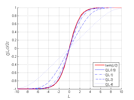
Figure 2: Plot of the function ฮถโ€‹(x;c)/2โ€‹c๐œ๐‘ฅ๐‘2๐‘\zeta(x;c)/2c with c๐‘c = 0.5, 1, 2, and 4. With c<0.5๐‘0.5c<0.5, ฮถโ€‹(x;c)/2โ€‹c๐œ๐‘ฅ๐‘2๐‘\zeta(x;c)/2c can be approximated to โˆ’tanhโก(x/2)๐‘ฅ2-\tanh(x/2).

Refer to caption

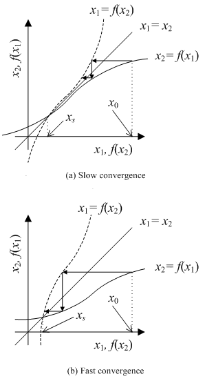
Figure 3: Two examples showing the convergence in lemma 1. The condition fโ€ฒ(x)|<1f^{\prime}(x)|<1 ensures the convergence to xssubscript๐‘ฅ๐‘ x_{s}, regardless of its convergence speed.

III-C Convergence proof for binary input

To prove the convergence of the forward-backward recursion in (25) for binary input, we first prove the following lemma.

Lemma 2

Let fโ€‹(x)๐‘“๐‘ฅf(x) be a function with the following two properties

  1. 1.

    fโ€‹(x)๐‘“๐‘ฅf(x) is a monotonic (either increasing or decreasing) function defined on (โˆ’โˆž,โˆž-\infty,\infty).

  2. 2.

    |fโ€ฒโ€‹(x)|<1superscript๐‘“โ€ฒ๐‘ฅ1|f^{\prime}(x)|<1 โˆ€xfor-all๐‘ฅ\forall x.

Then, the following properties hold

  1. 3.

    The equation, fโ€‹(x)=x๐‘“๐‘ฅ๐‘ฅf(x)=x, has a unique solution.

  2. 4.

    Let xssubscript๐‘ฅ๐‘ x_{s} be the solution of fโ€‹(x)=x๐‘“๐‘ฅ๐‘ฅf(x)=x. Let xksubscript๐‘ฅ๐‘˜x_{k} for k=1,2,3โ€‹โ‹ฏ๐‘˜123โ‹ฏk=1,2,3\cdots be a sequence obtained by successively applying f๐‘“f starting from an initial value x0subscript๐‘ฅ0x_{0}, i.e., xk=fโ€‹(xkโˆ’1)subscript๐‘ฅ๐‘˜๐‘“subscript๐‘ฅ๐‘˜1x_{k}=f(x_{k-1}). Then, for any x0subscript๐‘ฅ0x_{0}, xksubscript๐‘ฅ๐‘˜x_{k} approaches to xssubscript๐‘ฅ๐‘ x_{s} as kโ†’โˆžโ†’๐‘˜k\to\infty.

  3. 5.

    Let gโ€‹(x)=cโ‹…fโ€‹(xโˆ’a)+b๐‘”๐‘ฅโ‹…๐‘๐‘“๐‘ฅ๐‘Ž๐‘g(x)=c\cdot f(x-a)+b for some real values a๐‘Ža, b๐‘b and โˆ’1โ‰คcโ‰ค11๐‘1-1\leq c\leq 1. The properties 1) to 4) also hold for gโ€‹(x)๐‘”๐‘ฅg(x).

Proof:

Property 3) is obvious from 1) and 2). Proof of 4) is as follows. Let xkโˆ’1=xs+ฮ”kโˆ’1subscript๐‘ฅ๐‘˜1subscript๐‘ฅ๐‘ subscriptฮ”๐‘˜1x_{k-1}=x_{s}+\Delta_{k-1} and xk=fโ€‹(xs+ฮ”kโˆ’1)=xs+ฮ”ksubscript๐‘ฅ๐‘˜๐‘“subscript๐‘ฅ๐‘ subscriptฮ”๐‘˜1subscript๐‘ฅ๐‘ subscriptฮ”๐‘˜x_{k}=f(x_{s}+\Delta_{k-1})=x_{s}+\Delta_{k}. Suppose that ฮ”kโˆ’1>0subscriptฮ”๐‘˜10\Delta_{k-1}>0. Then, we have

|ฮ”k|subscriptฮ”๐‘˜\displaystyle|\Delta_{k}| =|โˆซxsxs+ฮ”kโˆ’1fโ€ฒโ€‹(x)โ€‹dx|absentsuperscriptsubscriptsubscript๐‘ฅ๐‘ subscript๐‘ฅ๐‘ subscriptฮ”๐‘˜1superscript๐‘“โ€ฒ๐‘ฅdifferential-d๐‘ฅ\displaystyle=\left|\int_{x_{s}}^{x_{s}+\Delta_{k-1}}f^{\prime}(x){\mathrm{d}}x\right|
=(a)โ€‹โˆซxsxs+ฮ”kโˆ’1|fโ€ฒโ€‹(x)|โ€‹dx๐‘Žsuperscriptsubscriptsubscript๐‘ฅ๐‘ subscript๐‘ฅ๐‘ subscriptฮ”๐‘˜1superscript๐‘“โ€ฒ๐‘ฅdifferential-d๐‘ฅ\displaystyle\overset{(a)}{=}\int_{x_{s}}^{x_{s}+\Delta_{k-1}}\left|f^{\prime}(x)\right|{\mathrm{d}}x
<(b)โ€‹โˆซxsxs+ฮ”kโˆ’1dx=ฮ”kโˆ’1=|ฮ”kโˆ’1|๐‘superscriptsubscriptsubscript๐‘ฅ๐‘ subscript๐‘ฅ๐‘ subscriptฮ”๐‘˜1differential-d๐‘ฅsubscriptฮ”๐‘˜1subscriptฮ”๐‘˜1\displaystyle\overset{(b)}{<}\int_{x_{s}}^{x_{s}+\Delta_{k-1}}{\mathrm{d}}x=\Delta_{k-1}=|\Delta_{k-1}|

where (a) is due to the monotony of fโ€‹(x)๐‘“๐‘ฅf(x), by which fโ€ฒโ€‹(x)superscript๐‘“โ€ฒ๐‘ฅf^{\prime}(x) always has the same sign, and (b) is due to |fโ€ฒโ€‹(x)|<1โ€‹โˆ€xsuperscript๐‘“โ€ฒ๐‘ฅ1for-all๐‘ฅ|f^{\prime}(x)|<1\;\forall x. Similarly, one also can show the same result, |ฮ”k|<|ฮ”kโˆ’1|subscriptฮ”๐‘˜subscriptฮ”๐‘˜1|\Delta_{k}|<|\Delta_{k-1}|, for ฮ”kโˆ’1<0subscriptฮ”๐‘˜10\Delta_{k-1}<0, which ensures that xโˆžโ†’xsโ†’subscript๐‘ฅsubscript๐‘ฅ๐‘ x_{\infty}\to x_{s}.

In 4), it is obvious that gโ€‹(x)๐‘”๐‘ฅg(x) also has the properties 1) and 2) since shift does not alter the slope and, with โˆ’1โ‰คcโ‰ค+11๐‘1-1\leq c\leq+1, |gโ€ฒโ€‹(x)|=|cโ€‹fโ€ฒโ€‹(xโˆ’a)|โ‰ค1superscript๐‘”โ€ฒ๐‘ฅ๐‘superscript๐‘“โ€ฒ๐‘ฅ๐‘Ž1|g^{\prime}(x)|=|cf^{\prime}(x-a)|\leq 1. Hence, 3) and 4) also hold for gโ€‹(x)๐‘”๐‘ฅg(x). โˆŽ

Fig.3(a) and (b) show two examples of the convergence in lemma 2 (Property 4)). From lemma 2, one can prove the convergence of the forward-backward recursion for binary input as follows.

Theorem 3

The forward and backward recursion in (25) for binary input converges to a unique fixed point as iteration goes to infinity.

Proof:

Note that the forward recursion at the j๐‘—jth node is of a form

ljโˆ’1โ†’jsubscript๐‘™โ†’๐‘—1๐‘—\displaystyle l_{j-1\to j} =gjโ€‹(ljโˆ’2โ†’jโˆ’1)โ‰กbjโˆ’ฮถโ€‹(ljโˆ’2โ†’jโˆ’1โˆ’aj;cj)absentsubscript๐‘”๐‘—subscript๐‘™โ†’๐‘—2๐‘—1subscript๐‘๐‘—๐œsubscript๐‘™โ†’๐‘—2๐‘—1subscript๐‘Ž๐‘—subscript๐‘๐‘—\displaystyle=g_{j}(l_{j-2\to j-1})\equiv b_{j}-\zeta(l_{j-2\to j-1}-a_{j};c_{j})

for some real values, ajsubscript๐‘Ž๐‘—a_{j}, bjsubscript๐‘๐‘—b_{j} and cjsubscript๐‘๐‘—c_{j}, where ฮถโ€‹(โ‹…)๐œโ‹…\zeta(\cdot) satisfies the properties 1) to 5) in lemma 2 and, hence, so is gjโ€‹(โ‹…)subscript๐‘”๐‘—โ‹…g_{j}(\cdot). Define one iteration as one complete turn of the recursions along the ring, such that the LLR of the j๐‘—jth data bit at the k๐‘˜kth iteration, ljโˆ’1โ†’j(k)superscriptsubscript๐‘™โ†’๐‘—1๐‘—๐‘˜l_{j-1\to j}^{(k)}, is represented as

ljโˆ’1โ†’j(k)superscriptsubscript๐‘™โ†’๐‘—1๐‘—๐‘˜\displaystyle l_{j-1\to j}^{(k)} =gT,jโ€‹(ljโˆ’1โ†’j(kโˆ’1))absentsubscript๐‘”๐‘‡๐‘—superscriptsubscript๐‘™โ†’๐‘—1๐‘—๐‘˜1\displaystyle=g_{T,j}(l_{j-1\to j}^{(k-1)})
=gjโˆ˜gjโˆ’1โˆ˜โ‹ฏโˆ˜g1โˆ˜gMโˆ˜โ€ฆโ€‹gj+1โ€‹(ljโˆ’1โ†’j(kโˆ’1))absentsubscript๐‘”๐‘—subscript๐‘”๐‘—1โ‹ฏsubscript๐‘”1subscript๐‘”๐‘€โ€ฆsubscript๐‘”๐‘—1superscriptsubscript๐‘™โ†’๐‘—1๐‘—๐‘˜1\displaystyle=g_{j}\circ g_{j-1}\circ\dots\circ g_{1}\circ g_{M}\circ\dots g_{j+1}(l_{j-1\to j}^{(k-1)})

where, from the chain rule, we have

dโ€‹gT,jdโ€‹ldsubscript๐‘”๐‘‡๐‘—d๐‘™\displaystyle\frac{{\mathrm{d}}g_{T,j}}{{\mathrm{d}}l} =dโ€‹gjdโ€‹gjโˆ’1โ‹…dโ€‹gjโˆ’1dโ€‹gjโˆ’2โ€‹โ‹ฏโ€‹dโ€‹g1dโ€‹gMโ‹…dโ€‹gMdโ€‹gMโˆ’1โ€‹โ‹ฏโ€‹dโ€‹gj+1dโ€‹labsentโ‹…โ‹…dsubscript๐‘”๐‘—dsubscript๐‘”๐‘—1dsubscript๐‘”๐‘—1dsubscript๐‘”๐‘—2โ‹ฏdsubscript๐‘”1dsubscript๐‘”๐‘€dsubscript๐‘”๐‘€dsubscript๐‘”๐‘€1โ‹ฏdsubscript๐‘”๐‘—1d๐‘™\displaystyle=\frac{{\mathrm{d}}g_{j}}{{\mathrm{d}}g_{j-1}}\cdot\frac{{\mathrm{d}}g_{j-1}}{{\mathrm{d}}g_{j-2}}\cdots\frac{{\mathrm{d}}g_{1}}{{\mathrm{d}}g_{M}}\cdot\frac{{\mathrm{d}}g_{M}}{{\mathrm{d}}g_{M-1}}\cdots\frac{{\mathrm{d}}g_{j+1}}{{\mathrm{d}}l}

Since all gjโ€‹(โ‹…)subscript๐‘”๐‘—โ‹…g_{j}(\cdot)โ€™s satisfy the properties 1) and 2) in lemma 2, so is gT,jโ€‹(โ‹…)subscript๐‘”๐‘‡๐‘—โ‹…g_{T,j}(\cdot). And, hence, from 3) to 5), ljโˆ’2โ†’jโˆ’1(k)superscriptsubscript๐‘™โ†’๐‘—2๐‘—1๐‘˜l_{j-2\to j-1}^{(k)} converges to a unique fixed point as kโ†’โˆžโ†’๐‘˜k\to\infty.

The convergence of the backward recursion can be proved similarly. Note that the two fixed points from the forward and backward recursion do not necessarily equal. โˆŽ

IV SINR Analysis via Density Evolution

In this section, we use the model in Section III-B to determine the stationary distribution of the LLR, ljโˆ’1โ†’jsubscript๐‘™โ†’๐‘—1๐‘—l_{j-1\to j}. Assuming the channel matrix ๐‘ฏ๐‘ฏ{\boldsymbol{H}} and the noise power ฯƒ2superscript๐œŽ2\sigma^{2} are fixed, we develop the density evolution of messages between neighboring nodes. In channel coding context, the density evolution in an iterative decoder assumes all-zero sequence is sent and the LLR mean is tracked with the number of iterations, assuming the LLR is Gaussian with its variance being the same as its mean. The density evolution used in [5] assumes the same, even though the approach differs.

In this section, we will also assume the LLRs are Gaussian and will track their mean and variance. The differences here from those in iterative channel decoding are that 1) both mean and variance have to be tracked along the ring, where the message of each node has different statistics and, hence, 2) we cannot assume all-zero input since the statistics of the current message, ljโˆ’1โ†’jsubscript๐‘™โ†’๐‘—1๐‘—l_{j-1\to j}, depends not only on the background noise but also on the other data. Fortunately, symmetry holds for binary data and the message depends largely on the previous data only so that one can proceed as follows: Under symmetry, we denote the mean and variance of ljโˆ’1โ†’jsubscript๐‘™โ†’๐‘—1๐‘—l_{j-1\to j} as mj|jโˆ’1โ€‹xjsubscript๐‘šconditional๐‘—๐‘—1subscript๐‘ฅ๐‘—m_{j|j-1}x_{j} and vj|jโˆ’1subscript๐‘ฃconditional๐‘—๐‘—1v_{j|j-1}, where both mj|jโˆ’1subscript๐‘šconditional๐‘—๐‘—1m_{j|j-1} and vj|jโˆ’1subscript๐‘ฃconditional๐‘—๐‘—1v_{j|j-1} are non-negative and the mean mj|jโˆ’1โ€‹xjsubscript๐‘šconditional๐‘—๐‘—1subscript๐‘ฅ๐‘—m_{j|j-1}x_{j} has the same sign as that of xjsubscript๐‘ฅ๐‘—x_{j}. In this definition, mj|jโˆ’1subscript๐‘šconditional๐‘—๐‘—1m_{j|j-1} can be interpreted as a reliability of ljโˆ’1โ†’jsubscript๐‘™โ†’๐‘—1๐‘—l_{j-1\to j}. Then, supposing that xj=+1subscript๐‘ฅ๐‘—1x_{j}=+1, we evaluate (mj|jโˆ’1,vj|jโˆ’1)subscript๐‘šconditional๐‘—๐‘—1subscript๐‘ฃconditional๐‘—๐‘—1(m_{j|j-1},v_{j|j-1}) for given (mjโˆ’1|jโˆ’2,vjโˆ’1|jโˆ’2)subscript๐‘š๐‘—conditional1๐‘—2subscript๐‘ฃ๐‘—conditional1๐‘—2(m_{j-1|j-2},v_{j-1|j-2}).

Assume uniform priors, i.e., la,j=0โ€‹โˆ€jsubscript๐‘™๐‘Ž๐‘—0for-all๐‘—l_{a,j}=0\;\forall j and suppose that xj=+1subscript๐‘ฅ๐‘—1x_{j}=+1. Using (5), the forward message passing in (25) becomes

ljโˆ’1โ†’jsubscript๐‘™โ†’๐‘—1๐‘—\displaystyle l_{j-1\to j} =4โ€‹yj|jโˆ’1(R)โˆ’ฮถโ€‹(ljโˆ’2โ†’jโˆ’1+2โ€‹dj|jโˆ’1;2โ€‹aj|jโˆ’1,jโˆ’1(R))absent4superscriptsubscript๐‘ฆconditional๐‘—๐‘—1๐‘…๐œsubscript๐‘™โ†’๐‘—2๐‘—12subscript๐‘‘conditional๐‘—๐‘—12superscriptsubscript๐‘Žconditional๐‘—๐‘—1๐‘—1๐‘…\displaystyle=4y_{j|j-1}^{(R)}-\zeta(l_{j-2\to j-1}+2d_{j|j-1};2a_{j|j-1,j-1}^{(R)})
=4โ€‹aj|jโˆ’1,j(R)+4โ€‹nj|jโˆ’1(R)+4โ€‹aj|jโˆ’1,jโˆ’1(R)โ€‹xjโˆ’1absent4superscriptsubscript๐‘Žconditional๐‘—๐‘—1๐‘—๐‘…4superscriptsubscript๐‘›conditional๐‘—๐‘—1๐‘…4superscriptsubscript๐‘Žconditional๐‘—๐‘—1๐‘—1๐‘…subscript๐‘ฅ๐‘—1\displaystyle=4a_{j|j-1,j}^{(R)}+4n_{j|j-1}^{(R)}+4a_{j|j-1,j-1}^{(R)}x_{j-1}
โˆ’ฮถโ€‹(ljโˆ’2โ†’jโˆ’1+2โ€‹dj|jโˆ’1;2โ€‹aj|jโˆ’1,jโˆ’1(R))๐œsubscript๐‘™โ†’๐‘—2๐‘—12subscript๐‘‘conditional๐‘—๐‘—12superscriptsubscript๐‘Žconditional๐‘—๐‘—1๐‘—1๐‘…\displaystyle-\zeta(l_{j-2\to j-1}+2d_{j|j-1};2a_{j|j-1,j-1}^{(R)})
=4โ€‹aj|jโˆ’1,j(R)+4โ€‹nj|jโˆ’1(R)+4โ€‹aj|jโˆ’1,jโˆ’1(R)โ€‹ejโˆ’1|jโˆ’2โ€‹(xjโˆ’1)absent4superscriptsubscript๐‘Žconditional๐‘—๐‘—1๐‘—๐‘…4superscriptsubscript๐‘›conditional๐‘—๐‘—1๐‘…4superscriptsubscript๐‘Žconditional๐‘—๐‘—1๐‘—1๐‘…subscript๐‘’๐‘—conditional1๐‘—2subscript๐‘ฅ๐‘—1\displaystyle=4a_{j|j-1,j}^{(R)}+4n_{j|j-1}^{(R)}+4a_{j|j-1,j-1}^{(R)}e_{j-1|j-2}(x_{j-1})
=4โ€‹zj|jโˆ’1+4โ€‹aj|jโˆ’1,jโˆ’1(R)โ€‹ejโˆ’1|jโˆ’2โ€‹(xjโˆ’1)absent4subscript๐‘งconditional๐‘—๐‘—14superscriptsubscript๐‘Žconditional๐‘—๐‘—1๐‘—1๐‘…subscript๐‘’๐‘—conditional1๐‘—2subscript๐‘ฅ๐‘—1\displaystyle=4z_{j|j-1}+4a_{j|j-1,j-1}^{(R)}e_{j-1|j-2}(x_{j-1}) (33)

where, from (26) to (28),

zj|jโˆ’1=subscript๐‘งconditional๐‘—๐‘—1absent\displaystyle z_{j|j-1}= aj|jโˆ’1,j(R)+nj|jโˆ’1(R)superscriptsubscript๐‘Žconditional๐‘—๐‘—1๐‘—๐‘…superscriptsubscript๐‘›conditional๐‘—๐‘—1๐‘…\displaystyle a_{j|j-1,j}^{(R)}+n_{j|j-1}^{(R)} (34)
yj|jโˆ’1(R)=superscriptsubscript๐‘ฆconditional๐‘—๐‘—1๐‘…absent\displaystyle y_{j|j-1}^{(R)}= aj|jโˆ’1,j(R)+nj|jโˆ’1(R)+aj|jโˆ’1,jโˆ’1(R)โ€‹xjโˆ’1superscriptsubscript๐‘Žconditional๐‘—๐‘—1๐‘—๐‘…superscriptsubscript๐‘›conditional๐‘—๐‘—1๐‘…superscriptsubscript๐‘Žconditional๐‘—๐‘—1๐‘—1๐‘…subscript๐‘ฅ๐‘—1\displaystyle a_{j|j-1,j}^{(R)}+n_{j|j-1}^{(R)}+a_{j|j-1,j-1}^{(R)}x_{j-1}
=\displaystyle= zj|jโˆ’1+aj|jโˆ’1,jโˆ’1(R)โ€‹xjโˆ’1subscript๐‘งconditional๐‘—๐‘—1superscriptsubscript๐‘Žconditional๐‘—๐‘—1๐‘—1๐‘…subscript๐‘ฅ๐‘—1\displaystyle z_{j|j-1}+a_{j|j-1,j-1}^{(R)}x_{j-1} (35)
ejโˆ’1|jโˆ’2subscript๐‘’๐‘—conditional1๐‘—2\displaystyle e_{j-1|j-2} (xjโˆ’1)=xjโˆ’1โˆ’ฮถโ€‹(ljโˆ’2โ†’jโˆ’1+2โ€‹dj|jโˆ’1;2โ€‹aj|jโˆ’1,jโˆ’1(R))4โ€‹aj|jโˆ’1,jโˆ’1(R)subscript๐‘ฅ๐‘—1subscript๐‘ฅ๐‘—1๐œsubscript๐‘™โ†’๐‘—2๐‘—12subscript๐‘‘conditional๐‘—๐‘—12superscriptsubscript๐‘Žconditional๐‘—๐‘—1๐‘—1๐‘…4superscriptsubscript๐‘Žconditional๐‘—๐‘—1๐‘—1๐‘…\displaystyle(x_{j-1})=x_{j-1}-\frac{\zeta(l_{j-2\to j-1}+2d_{j|j-1};2a_{j|j-1,j-1}^{(R)})}{4a_{j|j-1,j-1}^{(R)}} (36)
dj|jโˆ’1=subscript๐‘‘conditional๐‘—๐‘—1absent\displaystyle d_{j|j-1}= 2โ€‹aj|jโˆ’1,jโˆ’1(R)ฯƒj|jโˆ’12โ€‹(aj|jโˆ’1,j(R)+nj|jโˆ’1(R))2subscriptsuperscript๐‘Ž๐‘…conditional๐‘—๐‘—1๐‘—1subscriptsuperscript๐œŽ2conditional๐‘—๐‘—1subscriptsuperscript๐‘Ž๐‘…conditional๐‘—๐‘—1๐‘—subscriptsuperscript๐‘›๐‘…conditional๐‘—๐‘—1\displaystyle\frac{2a^{(R)}_{j|j-1,j-1}}{\sigma^{2}_{j|j-1}}\left(a^{(R)}_{j|j-1,j}+n^{(R)}_{j|j-1}\right)
+\displaystyle+ 2โ€‹|aj|jโˆ’1,jโˆ’1|2ฯƒj|jโˆ’12โ€‹xjโˆ’1+2โ€‹aj|jโˆ’1,jโˆ’1(I)ฯƒj|jโˆ’12โ€‹nj|jโˆ’1(I)2superscriptsubscript๐‘Žconditional๐‘—๐‘—1๐‘—12subscriptsuperscript๐œŽ2conditional๐‘—๐‘—1subscript๐‘ฅ๐‘—12subscriptsuperscript๐‘Ž๐ผconditional๐‘—๐‘—1๐‘—1subscriptsuperscript๐œŽ2conditional๐‘—๐‘—1subscriptsuperscript๐‘›๐ผconditional๐‘—๐‘—1\displaystyle\frac{2|a_{j|j-1,j-1}|^{2}}{\sigma^{2}_{j|j-1}}x_{j-1}+\frac{2a^{(I)}_{j|j-1,j-1}}{\sigma^{2}_{j|j-1}}n^{(I)}_{j|j-1}
=\displaystyle= 2โ€‹aj|jโˆ’1,jโˆ’1(R)ฯƒj|jโˆ’12โ€‹zj|jโˆ’1+2โ€‹|aj|jโˆ’1,jโˆ’1|2ฯƒj|jโˆ’12โ€‹xjโˆ’12subscriptsuperscript๐‘Ž๐‘…conditional๐‘—๐‘—1๐‘—1subscriptsuperscript๐œŽ2conditional๐‘—๐‘—1subscript๐‘งconditional๐‘—๐‘—12superscriptsubscript๐‘Žconditional๐‘—๐‘—1๐‘—12subscriptsuperscript๐œŽ2conditional๐‘—๐‘—1subscript๐‘ฅ๐‘—1\displaystyle\frac{2a^{(R)}_{j|j-1,j-1}}{\sigma^{2}_{j|j-1}}z_{j|j-1}+\frac{2|a_{j|j-1,j-1}|^{2}}{\sigma^{2}_{j|j-1}}x_{j-1}
+\displaystyle+ 2โ€‹aj|jโˆ’1,jโˆ’1(I)ฯƒj|jโˆ’12โ€‹nj|jโˆ’1(I)2subscriptsuperscript๐‘Ž๐ผconditional๐‘—๐‘—1๐‘—1subscriptsuperscript๐œŽ2conditional๐‘—๐‘—1subscriptsuperscript๐‘›๐ผconditional๐‘—๐‘—1\displaystyle\frac{2a^{(I)}_{j|j-1,j-1}}{\sigma^{2}_{j|j-1}}n^{(I)}_{j|j-1} (37)

Note that ejโˆ’1|jโˆ’2โ€‹(xjโˆ’1)subscript๐‘’๐‘—conditional1๐‘—2subscript๐‘ฅ๐‘—1e_{j-1|j-2}(x_{j-1}) is the estimation error on xjโˆ’1subscript๐‘ฅ๐‘—1x_{j-1} based on the information provided from the current observation, yj|jโˆ’1subscript๐‘ฆconditional๐‘—๐‘—1y_{j|j-1} and the previous node message, ljโˆ’2โ†’jโˆ’1subscript๐‘™โ†’๐‘—2๐‘—1l_{j-2\to j-1}.

IV-A Density evolution of the forward-backward recursion

Here, we determine (mj|jโˆ’1,vj|jโˆ’1)subscript๐‘šconditional๐‘—๐‘—1subscript๐‘ฃconditional๐‘—๐‘—1(m_{j|j-1},v_{j|j-1}) for given (mjโˆ’1|jโˆ’2,vjโˆ’1|jโˆ’2)subscript๐‘š๐‘—conditional1๐‘—2subscript๐‘ฃ๐‘—conditional1๐‘—2(m_{j-1|j-2},v_{j-1|j-2}) of the previous message, ljโˆ’2โ†’jโˆ’1subscript๐‘™โ†’๐‘—2๐‘—1l_{j-2\to j-1}. If the two terms in the last line of (33) is uncorrelated, the problem is simple. That is, we simply assume the estimation error, ejโˆ’1|jโˆ’2โ€‹(xjโˆ’1)subscript๐‘’๐‘—conditional1๐‘—2subscript๐‘ฅ๐‘—1e_{j-1|j-2}(x_{j-1}), is Gaussian, evaluate its mean and variance and add them to the mean and variance of zj|jโˆ’1subscript๐‘งconditional๐‘—๐‘—1z_{j|j-1}. By iterating such procedure many times, one can obtain the mean and variance of ljโˆ’1โ†’jsubscript๐‘™โ†’๐‘—1๐‘—l_{j-1\to j} (density evolution), even though we need numerical evaluation of integrals. Unfortunately, the two term are correlated due to 1) the inclusion of zj|jโˆ’1subscript๐‘งconditional๐‘—๐‘—1z_{j|j-1} in the argument of ฮถโ€‹(โ‹…)๐œโ‹…\zeta(\cdot) and 2) the noise + interference in the term zj|jโˆ’1subscript๐‘งconditional๐‘—๐‘—1z_{j|j-1} in ljโˆ’1โ†’jsubscript๐‘™โ†’๐‘—1๐‘—l_{j-1\to j} and zjโˆ’1|jโˆ’2โ€‹(xjโˆ’1)subscript๐‘ง๐‘—conditional1๐‘—2subscript๐‘ฅ๐‘—1z_{j-1|j-2}(x_{j-1}) in ljโˆ’2โ†’jโˆ’1subscript๐‘™โ†’๐‘—2๐‘—1l_{j-2\to j-1} are correlated. (Here, the dependency on xjโˆ’1subscript๐‘ฅ๐‘—1x_{j-1} is shown explicitly for zjโˆ’1|jโˆ’2subscript๐‘ง๐‘—conditional1๐‘—2z_{j-1|j-2}. While, it is not for zj|jโˆ’1subscript๐‘งconditional๐‘—๐‘—1z_{j|j-1} since we are assuming xj=+1subscript๐‘ฅ๐‘—1x_{j}=+1.) One thing that helps make the analysis possible is that they both are well modeled as Gaussian so that the density evolution is numerically tractable by making a few simplifying assumptions.

To this end, we fix xjโˆ’1subscript๐‘ฅ๐‘—1x_{j-1} and explore the correlations between the involving variables, of which the randomness solely comes from the noise and other interferences than xjsubscript๐‘ฅ๐‘—x_{j} and xjโˆ’1subscript๐‘ฅ๐‘—1x_{j-1}. Consider first zj|jโˆ’1subscript๐‘งconditional๐‘—๐‘—1z_{j|j-1} in the last line of (33). We have, from (6) and (7),

zj|jโˆ’1subscript๐‘งconditional๐‘—๐‘—1\displaystyle z_{j|j-1} โˆผ๐’ฉโ€‹(aj|jโˆ’1,j(R),๐”ผโ€‹(nj|jโˆ’1(R))2)similar-toabsent๐’ฉsubscriptsuperscript๐‘Ž๐‘…conditional๐‘—๐‘—1๐‘—๐”ผsuperscriptsubscriptsuperscript๐‘›๐‘…conditional๐‘—๐‘—12\displaystyle\sim{\mathcal{N}}\left(a^{(R)}_{j|j-1,j},{\mathbb{E}}(n^{(R)}_{j|j-1})^{2}\right) (38)

where, if we assume the suppressed noise + interference, nj|jโˆ’1subscript๐‘›conditional๐‘—๐‘—1n_{j|j-1}, is circularly symmetric, then the variance is given, from (7) and (8), by

๐”ผโ€‹(nj|jโˆ’1(R))2๐”ผsuperscriptsubscriptsuperscript๐‘›๐‘…conditional๐‘—๐‘—12\displaystyle{\mathbb{E}}(n^{(R)}_{j|j-1})^{2} =๐”ผโ€‹(nj|jโˆ’1(I))2=aj|jโˆ’1,j(R)2absent๐”ผsuperscriptsubscriptsuperscript๐‘›๐ผconditional๐‘—๐‘—12subscriptsuperscript๐‘Ž๐‘…conditional๐‘—๐‘—1๐‘—2\displaystyle={\mathbb{E}}(n^{(I)}_{j|j-1})^{2}=\frac{a^{(R)}_{j|j-1,j}}{2} (39)

This is valid when circularly symmetric constellations, such as QPSK, are used, while it is generally not for non-circularly symmetric real constellations, such as BPSK. Although it has little impact, especially when M๐‘€M is large, it will be certainly more accurate to use the exact variances, which are given in Appendix A.

Now, let us look at the argument of ฮถโ€‹(โ‹…)๐œโ‹…\zeta(\cdot), which can be rewritten as

ljโˆ’2โ†’jโˆ’1subscript๐‘™โ†’๐‘—2๐‘—1\displaystyle l_{j-2\to j-1} +2โ€‹dj|jโˆ’1=ljโˆ’2โ†’jโˆ’1+4โ€‹aj|jโˆ’1,jโˆ’1(R)ฯƒj|jโˆ’12โ€‹zj|jโˆ’12subscript๐‘‘conditional๐‘—๐‘—1subscript๐‘™โ†’๐‘—2๐‘—14subscriptsuperscript๐‘Ž๐‘…conditional๐‘—๐‘—1๐‘—1subscriptsuperscript๐œŽ2conditional๐‘—๐‘—1subscript๐‘งconditional๐‘—๐‘—1\displaystyle+2d_{j|j-1}=l_{j-2\to j-1}+\frac{4a^{(R)}_{j|j-1,j-1}}{\sigma^{2}_{j|j-1}}z_{j|j-1}
+4โ€‹|aj|jโˆ’1,jโˆ’1|2ฯƒj|jโˆ’12โ€‹xjโˆ’1+4โ€‹aj|jโˆ’1,jโˆ’1(I)ฯƒj|jโˆ’12โ€‹nj|jโˆ’1(I)4superscriptsubscript๐‘Žconditional๐‘—๐‘—1๐‘—12subscriptsuperscript๐œŽ2conditional๐‘—๐‘—1subscript๐‘ฅ๐‘—14subscriptsuperscript๐‘Ž๐ผconditional๐‘—๐‘—1๐‘—1subscriptsuperscript๐œŽ2conditional๐‘—๐‘—1subscriptsuperscript๐‘›๐ผconditional๐‘—๐‘—1\displaystyle+\frac{4|a_{j|j-1,j-1}|^{2}}{\sigma^{2}_{j|j-1}}x_{j-1}+\frac{4a^{(I)}_{j|j-1,j-1}}{\sigma^{2}_{j|j-1}}n^{(I)}_{j|j-1} (40)

where ljโˆ’2โ†’jโˆ’1subscript๐‘™โ†’๐‘—2๐‘—1l_{j-2\to j-1} is assumed to be Gaussian, of which the mean and variance are provided from the previous node as the pair (mjโˆ’1|jโˆ’2,vjโˆ’1|jโˆ’2)subscript๐‘š๐‘—conditional1๐‘—2subscript๐‘ฃ๐‘—conditional1๐‘—2(m_{j-1|j-2},v_{j-1|j-2}), i.e.,

ljโˆ’2โ†’jโˆ’1subscript๐‘™โ†’๐‘—2๐‘—1\displaystyle l_{j-2\to j-1} โˆผ๐’ฉโ€‹(mjโˆ’1|jโˆ’2โ€‹xjโˆ’1,vjโˆ’1|jโˆ’2)similar-toabsent๐’ฉsubscript๐‘š๐‘—conditional1๐‘—2subscript๐‘ฅ๐‘—1subscript๐‘ฃ๐‘—conditional1๐‘—2\displaystyle\sim{\mathcal{N}}\left(m_{j-1|j-2}x_{j-1},v_{j-1|j-2}\right) (41)

The rest three terms, except for ljโˆ’2โ†’jโˆ’1subscript๐‘™โ†’๐‘—2๐‘—1l_{j-2\to j-1}, are assumed to be uncorrelated to each other. Although zj|jโˆ’1subscript๐‘งconditional๐‘—๐‘—1z_{j|j-1} has a weak correlation with nj|jโˆ’1(I)subscriptsuperscript๐‘›๐ผconditional๐‘—๐‘—1n^{(I)}_{j|j-1} as shown in the Appendix A, we will ignore it for analytical simplicity. Unfortunately, ljโˆ’2โ†’jโˆ’1subscript๐‘™โ†’๐‘—2๐‘—1l_{j-2\to j-1} and zj|jโˆ’1subscript๐‘งconditional๐‘—๐‘—1z_{j|j-1} has non-negligible covariance. Recalling the definition of zj|jโˆ’1subscript๐‘งconditional๐‘—๐‘—1z_{j|j-1} and ljโˆ’2โ†’jโˆ’1subscript๐‘™โ†’๐‘—2๐‘—1l_{j-2\to j-1}, it stems from the covariance between nj|jโˆ’1(R)subscriptsuperscript๐‘›๐‘…conditional๐‘—๐‘—1n^{(R)}_{j|j-1} in zj|jโˆ’1subscript๐‘งconditional๐‘—๐‘—1z_{j|j-1} and njโˆ’1|jโˆ’2(R)subscriptsuperscript๐‘›๐‘…๐‘—conditional1๐‘—2n^{(R)}_{j-1|j-2} in ljโˆ’2โ†’jโˆ’1subscript๐‘™โ†’๐‘—2๐‘—1l_{j-2\to j-1}, which is given by

ฯƒlโ€‹z,jsubscript๐œŽ๐‘™๐‘ง๐‘—\displaystyle\sigma_{lz,j} โ‰ก๐”ผโ€‹[ljโˆ’2โ†’jโˆ’1โ‹…zj|jโˆ’1|xjโˆ’1]absent๐”ผdelimited-[]conditionalโ‹…subscript๐‘™โ†’๐‘—2๐‘—1subscript๐‘งconditional๐‘—๐‘—1subscript๐‘ฅ๐‘—1\displaystyle\equiv{\mathbb{E}}\left[l_{j-2\to j-1}\cdot z_{j|j-1}|x_{j-1}\right]
โˆ’๐”ผโ€‹[ljโˆ’2โ†’jโˆ’1|xjโˆ’1]โ‹…๐”ผโ€‹[zj|jโˆ’1]โ‹…๐”ผdelimited-[]conditionalsubscript๐‘™โ†’๐‘—2๐‘—1subscript๐‘ฅ๐‘—1๐”ผdelimited-[]subscript๐‘งconditional๐‘—๐‘—1\displaystyle-{\mathbb{E}}\left[l_{j-2\to j-1}|x_{j-1}\right]\cdot{\mathbb{E}}\left[z_{j|j-1}\right]
=๐”ผโ€‹[nj|jโˆ’1(R)โ€‹njโˆ’1|jโˆ’2(R)]+2โ€‹ajโˆ’1|jโˆ’2(R)โ‹…๐”ผโ€‹[nj|jโˆ’1(R)โ€‹ejโˆ’1|jโˆ’2]absent๐”ผdelimited-[]subscriptsuperscript๐‘›๐‘…conditional๐‘—๐‘—1subscriptsuperscript๐‘›๐‘…๐‘—conditional1๐‘—2โ‹…2subscriptsuperscript๐‘Ž๐‘…๐‘—conditional1๐‘—2๐”ผdelimited-[]subscriptsuperscript๐‘›๐‘…conditional๐‘—๐‘—1subscript๐‘’๐‘—conditional1๐‘—2\displaystyle={\mathbb{E}}\left[n^{(R)}_{j|j-1}n^{(R)}_{j-1|j-2}\right]+2a^{(R)}_{j-1|j-2}\cdot{\mathbb{E}}\left[n^{(R)}_{j|j-1}e_{j-1|j-2}\right]
โ‰ˆ๐”ผโ€‹[nj|jโˆ’1(R)โ€‹njโˆ’1|jโˆ’2(R)]absent๐”ผdelimited-[]subscriptsuperscript๐‘›๐‘…conditional๐‘—๐‘—1subscriptsuperscript๐‘›๐‘…๐‘—conditional1๐‘—2\displaystyle\approx{\mathbb{E}}\left[n^{(R)}_{j|j-1}n^{(R)}_{j-1|j-2}\right] (42)

where we ignored the correlation between nj|jโˆ’1(R)subscriptsuperscript๐‘›๐‘…conditional๐‘—๐‘—1n^{(R)}_{j|j-1} and ejโˆ’1|jโˆ’2subscript๐‘’๐‘—conditional1๐‘—2e_{j-1|j-2}.

Noting that

๐”ผ๐”ผ\displaystyle{\mathbb{E}} [nj|jโˆ’1(R)โ€‹njโˆ’1|jโˆ’2(R)]+๐”ผโ€‹[nj|jโˆ’1(I)โ€‹njโˆ’1|jโˆ’2(I)]delimited-[]subscriptsuperscript๐‘›๐‘…conditional๐‘—๐‘—1subscriptsuperscript๐‘›๐‘…๐‘—conditional1๐‘—2๐”ผdelimited-[]subscriptsuperscript๐‘›๐ผconditional๐‘—๐‘—1subscriptsuperscript๐‘›๐ผ๐‘—conditional1๐‘—2\displaystyle\left[n^{(R)}_{j|j-1}n^{(R)}_{j-1|j-2}\right]+{\mathbb{E}}\left[n^{(I)}_{j|j-1}n^{(I)}_{j-1|j-2}\right]
=โ„œโก[nj|jโˆ’1โ€‹njโˆ’1|jโˆ’2โˆ—]absentsubscript๐‘›conditional๐‘—๐‘—1subscriptsuperscript๐‘›๐‘—conditional1๐‘—2\displaystyle=\Re\left[n_{j|j-1}n^{*}_{j-1|j-2}\right]
=โ„œโก[๐’‰jHโ€‹๐‘ฒ{j,jโˆ’1}โˆ’1โ€‹๐‘ฒ{j,jโˆ’1,jโˆ’2}โ€‹๐‘ฒ{jโˆ’1,jโˆ’2}โˆ’1โ€‹๐’‰jโˆ’1]absentsubscriptsuperscript๐’‰๐ป๐‘—subscriptsuperscript๐‘ฒ1๐‘—๐‘—1subscript๐‘ฒ๐‘—๐‘—1๐‘—2subscriptsuperscript๐‘ฒ1๐‘—1๐‘—2subscript๐’‰๐‘—1\displaystyle=\Re\left[{\boldsymbol{h}}^{H}_{j}{\boldsymbol{K}}^{-1}_{\{j,j-1\}}{\boldsymbol{K}}_{\{j,j-1,j-2\}}{\boldsymbol{K}}^{-1}_{\{j-1,j-2\}}{\boldsymbol{h}}_{j-1}\right] (43)

and resorting to the circular symmetry, we have

๐”ผโ€‹[nj|jโˆ’1(R)โ€‹njโˆ’1|jโˆ’2(R)]=๐”ผโ€‹[nj|jโˆ’1(I)โ€‹njโˆ’1|jโˆ’2(I)],๐”ผdelimited-[]subscriptsuperscript๐‘›๐‘…conditional๐‘—๐‘—1subscriptsuperscript๐‘›๐‘…๐‘—conditional1๐‘—2๐”ผdelimited-[]subscriptsuperscript๐‘›๐ผconditional๐‘—๐‘—1subscriptsuperscript๐‘›๐ผ๐‘—conditional1๐‘—2\displaystyle{\mathbb{E}}\left[n^{(R)}_{j|j-1}n^{(R)}_{j-1|j-2}\right]={\mathbb{E}}\left[n^{(I)}_{j|j-1}n^{(I)}_{j-1|j-2}\right],

resulting in

ฯƒlโ€‹z,jsubscript๐œŽ๐‘™๐‘ง๐‘—\displaystyle\sigma_{lz,j} โ‰ˆ12โ€‹โ„œโก[๐’‰jHโ€‹๐‘ฒ{j,jโˆ’1}โˆ’1โ€‹๐‘ฒ{j,jโˆ’1,jโˆ’2}โ€‹๐‘ฒ{jโˆ’1,jโˆ’2}โˆ’1โ€‹๐’‰jโˆ’1]absent12subscriptsuperscript๐’‰๐ป๐‘—subscriptsuperscript๐‘ฒ1๐‘—๐‘—1subscript๐‘ฒ๐‘—๐‘—1๐‘—2subscriptsuperscript๐‘ฒ1๐‘—1๐‘—2subscript๐’‰๐‘—1\displaystyle\approx\frac{1}{2}\Re\left[{\boldsymbol{h}}^{H}_{j}{\boldsymbol{K}}^{-1}_{\{j,j-1\}}{\boldsymbol{K}}_{\{j,j-1,j-2\}}{\boldsymbol{K}}^{-1}_{\{j-1,j-2\}}{\boldsymbol{h}}_{j-1}\right] (44)

Without circular symmetry, we also may use similar derivation to ๐”ผโ€‹(nj|jโˆ’1(R))2๐”ผsuperscriptsubscriptsuperscript๐‘›๐‘…conditional๐‘—๐‘—12{\mathbb{E}}(n^{(R)}_{j|j-1})^{2} as shown in the Appendix A.

According to the argument below, one can rewrite (40) using two correlated random variables, say zj|jโˆ’1subscript๐‘งconditional๐‘—๐‘—1z_{j|j-1} and wj|jโˆ’1subscript๐‘คconditional๐‘—๐‘—1w_{j|j-1}, (conditioned on xjโˆ’1subscript๐‘ฅ๐‘—1x_{j-1}), i.e.,

l๐‘™\displaystyle l +jโˆ’2โ†’jโˆ’12dj|jโˆ’1{}_{j-2\to j-1}+2d_{j|j-1}
=โˆ˜โ€‹4โ€‹aj|jโˆ’1,jโˆ’1(R)ฯƒj|jโˆ’12โ€‹zj|jโˆ’1+4โ€‹|aj|jโˆ’1,jโˆ’1|2ฯƒj|jโˆ’12โ€‹xjโˆ’1+wj|jโˆ’14subscriptsuperscript๐‘Ž๐‘…conditional๐‘—๐‘—1๐‘—1subscriptsuperscript๐œŽ2conditional๐‘—๐‘—1subscript๐‘งconditional๐‘—๐‘—14superscriptsubscript๐‘Žconditional๐‘—๐‘—1๐‘—12subscriptsuperscript๐œŽ2conditional๐‘—๐‘—1subscript๐‘ฅ๐‘—1subscript๐‘คconditional๐‘—๐‘—1\displaystyle\overset{\circ}{=}\frac{4a^{(R)}_{j|j-1,j-1}}{\sigma^{2}_{j|j-1}}z_{j|j-1}+\frac{4|a_{j|j-1,j-1}|^{2}}{\sigma^{2}_{j|j-1}}x_{j-1}+w_{j|j-1} (45)

where =โˆ˜\overset{\circ}{=} represents equivalence in distribution and

wj|jโˆ’1subscript๐‘คconditional๐‘—๐‘—1\displaystyle w_{j|j-1} โ‰กljโˆ’2โ†’jโˆ’1+4โ€‹aj|jโˆ’1,jโˆ’1(I)ฯƒj|jโˆ’12โ€‹nj|jโˆ’1(I)absentsubscript๐‘™โ†’๐‘—2๐‘—14subscriptsuperscript๐‘Ž๐ผconditional๐‘—๐‘—1๐‘—1subscriptsuperscript๐œŽ2conditional๐‘—๐‘—1subscriptsuperscript๐‘›๐ผconditional๐‘—๐‘—1\displaystyle\equiv l_{j-2\to j-1}+\frac{4a^{(I)}_{j|j-1,j-1}}{\sigma^{2}_{j|j-1}}n^{(I)}_{j|j-1}
โˆผ๐’ฉโ€‹(mjโˆ’1|jโˆ’2โ€‹xjโˆ’1,vjโˆ’1|jโˆ’2+ฮฑ)similar-toabsent๐’ฉsubscript๐‘š๐‘—conditional1๐‘—2subscript๐‘ฅ๐‘—1subscript๐‘ฃ๐‘—conditional1๐‘—2๐›ผ\displaystyle\sim{\mathcal{N}}\left(m_{j-1|j-2}x_{j-1},v_{j-1|j-2}+\alpha\right) (46)

with

ฮฑ=(4โ€‹aj|jโˆ’1,jโˆ’1(I)ฯƒj|jโˆ’12)2โ€‹๐”ผโ€‹(nj|jโˆ’1(I))2๐›ผsuperscript4subscriptsuperscript๐‘Ž๐ผconditional๐‘—๐‘—1๐‘—1subscriptsuperscript๐œŽ2conditional๐‘—๐‘—12๐”ผsuperscriptsubscriptsuperscript๐‘›๐ผconditional๐‘—๐‘—12\displaystyle\alpha=\left(\frac{4a^{(I)}_{j|j-1,j-1}}{\sigma^{2}_{j|j-1}}\right)^{2}{\mathbb{E}}\left(n^{(I)}_{j|j-1}\right)^{2} (47)

Recalling the covariance between zj|jโˆ’1subscript๐‘งconditional๐‘—๐‘—1z_{j|j-1} and wj|jโˆ’1subscript๐‘คconditional๐‘—๐‘—1w_{j|j-1} given by (42), the mean and covariance of the Gaussian random pair (zj|jโˆ’1,wj|jโˆ’1)Tsuperscriptsubscript๐‘งconditional๐‘—๐‘—1subscript๐‘คconditional๐‘—๐‘—1๐‘‡(z_{j|j-1},w_{j|j-1})^{T} are given respectively by

๐j|jโˆ’1subscript๐conditional๐‘—๐‘—1\displaystyle{\boldsymbol{\mu}}_{j|j-1} =[aj|jโˆ’1,j(R)mjโˆ’1|jโˆ’2โ€‹xjโˆ’1]absentmatrixsubscriptsuperscript๐‘Ž๐‘…conditional๐‘—๐‘—1๐‘—subscript๐‘š๐‘—conditional1๐‘—2subscript๐‘ฅ๐‘—1\displaystyle=\begin{bmatrix}a^{(R)}_{j|j-1,j}\\[3.00003pt] m_{j-1|j-2}x_{j-1}\end{bmatrix} (48)
๐‘ชj|jโˆ’1subscript๐‘ชconditional๐‘—๐‘—1\displaystyle{\boldsymbol{C}}_{j|j-1} =[๐”ผโ€‹(nj|jโˆ’1(R))2ฯƒlโ€‹z,jฯƒlโ€‹z,jvjโˆ’1|jโˆ’2+ฮฑ]absentmatrix๐”ผsuperscriptsubscriptsuperscript๐‘›๐‘…conditional๐‘—๐‘—12subscript๐œŽ๐‘™๐‘ง๐‘—subscript๐œŽ๐‘™๐‘ง๐‘—subscript๐‘ฃ๐‘—conditional1๐‘—2๐›ผ\displaystyle=\begin{bmatrix}{\mathbb{E}}\left(n^{(R)}_{j|j-1}\right)^{2}&\sigma_{lz,j}\\[3.00003pt] \sigma_{lz,j}&v_{j-1|j-2}+\alpha\end{bmatrix} (49)

Now, the density evolution can be numerically evaluated by taking average over all possible triple (xjโˆ’1,zj|jโˆ’1,wj|jโˆ’1)subscript๐‘ฅ๐‘—1subscript๐‘งconditional๐‘—๐‘—1subscript๐‘คconditional๐‘—๐‘—1(x_{j-1},z_{j|j-1},w_{j|j-1}), i.e.,

mj|jโˆ’1subscript๐‘šconditional๐‘—๐‘—1\displaystyle m_{j|j-1} =๐”ผx,z,wโ€‹[Lj|jโˆ’1โ€‹(x,z,w)]absentsubscript๐”ผ๐‘ฅ๐‘ง๐‘คdelimited-[]subscript๐ฟconditional๐‘—๐‘—1๐‘ฅ๐‘ง๐‘ค\displaystyle={\mathbb{E}}_{x,z,w}\left[L_{j|j-1}(x,z,w)\right] (50)
vj|jโˆ’1subscript๐‘ฃconditional๐‘—๐‘—1\displaystyle v_{j|j-1} =๐”ผx,z,wโ€‹[Lj|jโˆ’1โ€‹(x,z,w)2]โˆ’mj|jโˆ’12absentsubscript๐”ผ๐‘ฅ๐‘ง๐‘คdelimited-[]subscript๐ฟconditional๐‘—๐‘—1superscript๐‘ฅ๐‘ง๐‘ค2superscriptsubscript๐‘šconditional๐‘—๐‘—12\displaystyle={\mathbb{E}}_{x,z,w}\left[L_{j|j-1}(x,z,w)^{2}\right]-m_{j|j-1}^{2} (51)

where

L๐ฟ\displaystyle L (x,z,w)j|jโˆ’1=4z+4aj|jโˆ’1,jโˆ’1(R)x{}_{j|j-1}(x,z,w)=4z+4a^{(R)}_{j|j-1,j-1}x
โˆ’ฮถโ€‹(4โ€‹aj|jโˆ’1,jโˆ’1(I)ฯƒj|jโˆ’12โ€‹z+4โ€‹|aj|jโˆ’1,jโˆ’1|2ฯƒj|jโˆ’12โ€‹x+w;aj|jโˆ’1,jโˆ’1(R))๐œ4subscriptsuperscript๐‘Ž๐ผconditional๐‘—๐‘—1๐‘—1subscriptsuperscript๐œŽ2conditional๐‘—๐‘—1๐‘ง4superscriptsubscript๐‘Žconditional๐‘—๐‘—1๐‘—12subscriptsuperscript๐œŽ2conditional๐‘—๐‘—1๐‘ฅ๐‘คsubscriptsuperscript๐‘Ž๐‘…conditional๐‘—๐‘—1๐‘—1\displaystyle-\zeta\left(\frac{4a^{(I)}_{j|j-1,j-1}}{\sigma^{2}_{j|j-1}}z+\frac{4|a_{j|j-1,j-1}|^{2}}{\sigma^{2}_{j|j-1}}x+w;a^{(R)}_{j|j-1,j-1}\right) (52)
๐”ผ๐”ผ\displaystyle{\mathbb{E}} [g(x,z,w)]x,z,w={}_{x,z,w}\left[g(x,z,w)\right]=
โˆ‘x=ยฑ112โ€‹โˆฌโˆ’โˆžโˆžgโ€‹(x,z,w)โ€‹ฮฆโ€‹((w,z)T;๐j|jโˆ’1,๐‘ชj|jโˆ’1)โ€‹dwโ€‹dzsubscript๐‘ฅplus-or-minus112superscriptsubscriptdouble-integral๐‘”๐‘ฅ๐‘ง๐‘คฮฆsuperscript๐‘ค๐‘ง๐‘‡subscript๐conditional๐‘—๐‘—1subscript๐‘ชconditional๐‘—๐‘—1differential-d๐‘คdifferential-d๐‘ง\displaystyle\sum_{x=\pm 1}\frac{1}{2}\displaystyle\iint_{-\infty}^{\infty}g(x,z,w)\Phi\left((w,z)^{T};{\boldsymbol{\mu}}_{j|j-1},{\boldsymbol{C}}_{j|j-1}\right){\mathrm{d}}w{\mathrm{d}}z (53)

and ฮฆโ€‹((w,z)T;๐,๐‘ช)ฮฆsuperscript๐‘ค๐‘ง๐‘‡๐๐‘ช\Phi((w,z)^{T};{\boldsymbol{\mu}},{\boldsymbol{C}}) is bi-variate Gaussian density function with mean ๐๐{\boldsymbol{\mu}} and covariance matrix ๐‘ช๐‘ช{\boldsymbol{C}}.

IV-B SINR of the final belief

The final belief is given by l^j=ljโˆ’1โ†’j+lj+1โ†’jsubscript^๐‘™๐‘—subscript๐‘™โ†’๐‘—1๐‘—subscript๐‘™โ†’๐‘—1๐‘—{\hat{l}}_{j}=l_{j-1\to j}+l_{j+1\to j}, for which the mean and variance are given by

๐”ผโ€‹[l^j]๐”ผdelimited-[]subscript^๐‘™๐‘—\displaystyle{\mathbb{E}}[{\hat{l}}_{j}] =mj|jโˆ’1+mj|j+1absentsubscript๐‘šconditional๐‘—๐‘—1subscript๐‘šconditional๐‘—๐‘—1\displaystyle=m_{j|j-1}+m_{j|j+1} (54)
๐•โ€‹arโ€‹[l^j]๐•ardelimited-[]subscript^๐‘™๐‘—\displaystyle{\mathbb{V}\rm{ar}}[{\hat{l}}_{j}] =vj|jโˆ’1+vj|j+1+2โ€‹๐”ผโ€‹[ljโˆ’1โ†’jโ€‹lj+1โ†’j]absentsubscript๐‘ฃconditional๐‘—๐‘—1subscript๐‘ฃconditional๐‘—๐‘—12๐”ผdelimited-[]subscript๐‘™โ†’๐‘—1๐‘—subscript๐‘™โ†’๐‘—1๐‘—\displaystyle=v_{j|j-1}+v_{j|j+1}+2{\mathbb{E}}[l_{j-1\to j}l_{j+1\to j}]
โˆ’2โ€‹mj|jโˆ’1โ€‹mj|j+12subscript๐‘šconditional๐‘—๐‘—1subscript๐‘šconditional๐‘—๐‘—1\displaystyle-2m_{j|j-1}m_{j|j+1} (55)

Since the two terms zj|jยฑ1subscript๐‘งconditional๐‘—plus-or-minus๐‘—1z_{j|j\pm 1} and ejยฑ1|jยฑ2subscript๐‘’plus-or-minus๐‘—conditional1plus-or-minus๐‘—2e_{j\pm 1|j\pm 2} in ljยฑ1โ†’jsubscript๐‘™โ†’plus-or-minus๐‘—1๐‘—l_{j\pm 1\to j} have correlation to each other, the computation of ๐”ผโ€‹[ljโˆ’1โ†’jโ€‹lj+1โ†’j]๐”ผdelimited-[]subscript๐‘™โ†’๐‘—1๐‘—subscript๐‘™โ†’๐‘—1๐‘—{\mathbb{E}}[l_{j-1\to j}l_{j+1\to j}] in (55) is little bit tricky. However, noting that ej+1|j+2subscript๐‘’๐‘—conditional1๐‘—2e_{j+1|j+2} and ejโˆ’1|jโˆ’2subscript๐‘’๐‘—conditional1๐‘—2e_{j-1|j-2} are conditionally independent for given zj|j+1subscript๐‘งconditional๐‘—๐‘—1z_{j|j+1} and zj|jโˆ’1subscript๐‘งconditional๐‘—๐‘—1z_{j|j-1}, it can be obtained as follows.

๐”ผโ€‹[ljโˆ’1โ†’jโ€‹lj+1โ†’j]๐”ผdelimited-[]subscript๐‘™โ†’๐‘—1๐‘—subscript๐‘™โ†’๐‘—1๐‘—\displaystyle{\mathbb{E}}[l_{j-1\to j}l_{j+1\to j}] =\displaystyle= (56)
โˆฌ๐”ผโ€‹[ljโˆ’1โ†’j|zf]double-integral๐”ผdelimited-[]conditionalsubscript๐‘™โ†’๐‘—1๐‘—subscript๐‘ง๐‘“\displaystyle\iint{\mathbb{E}}[l_{j-1\to j}|z_{f}] โ‹…๐”ผโ€‹[lj+1โ†’j|zb]โ€‹ฮฆโ€‹((zf,zb)T;๐z,j,๐‘ชzโ€‹z,j)โ€‹dโ€‹zfโ€‹dโ€‹zbโ‹…absent๐”ผdelimited-[]conditionalsubscript๐‘™โ†’๐‘—1๐‘—subscript๐‘ง๐‘ฮฆsuperscriptsubscript๐‘ง๐‘“subscript๐‘ง๐‘๐‘‡subscript๐๐‘ง๐‘—subscript๐‘ช๐‘ง๐‘ง๐‘—dsubscript๐‘ง๐‘“dsubscript๐‘ง๐‘\displaystyle\cdot{\mathbb{E}}[l_{j+1\to j}|z_{b}]\Phi\left((z_{f},z_{b})^{T};{\boldsymbol{\mu}}_{z,j},{\boldsymbol{C}}_{zz,j}\right){\mathrm{d}}z_{f}{\mathrm{d}}z_{b} (57)

where

๐z,jsubscript๐๐‘ง๐‘—\displaystyle{\boldsymbol{\mu}}_{z,j} =[aj|jโˆ’1,j(R)aj|j+1,j(R)]absentmatrixsubscriptsuperscript๐‘Ž๐‘…conditional๐‘—๐‘—1๐‘—subscriptsuperscript๐‘Ž๐‘…conditional๐‘—๐‘—1๐‘—\displaystyle=\begin{bmatrix}a^{(R)}_{j|j-1,j}\\[3.00003pt] a^{(R)}_{j|j+1,j}\end{bmatrix} (58)
๐‘ชzโ€‹z,jsubscript๐‘ช๐‘ง๐‘ง๐‘—\displaystyle{\boldsymbol{C}}_{zz,j} =[๐”ผโ€‹(nj|jโˆ’1(R))2ฯƒzโ€‹z,jฯƒzโ€‹z,j๐”ผโ€‹(nj|j+1(R))2]absentmatrix๐”ผsuperscriptsubscriptsuperscript๐‘›๐‘…conditional๐‘—๐‘—12subscript๐œŽ๐‘ง๐‘ง๐‘—subscript๐œŽ๐‘ง๐‘ง๐‘—๐”ผsuperscriptsubscriptsuperscript๐‘›๐‘…conditional๐‘—๐‘—12\displaystyle=\begin{bmatrix}{\mathbb{E}}\left(n^{(R)}_{j|j-1}\right)^{2}&\sigma_{zz,j}\\[3.00003pt] \sigma_{zz,j}&{\mathbb{E}}\left(n^{(R)}_{j|j+1}\right)^{2}\end{bmatrix} (59)
ฯƒzโ€‹z,jsubscript๐œŽ๐‘ง๐‘ง๐‘—\displaystyle\sigma_{zz,j} โ‰ˆ12โ€‹โ„œโก[๐’‰jHโ€‹๐‘ฒ{j,jโˆ’1}โˆ’1โ€‹๐‘ฒ{j+1,j,jโˆ’1}โ€‹๐‘ฒ{j,j+1}โˆ’1โ€‹๐’‰j]absent12subscriptsuperscript๐’‰๐ป๐‘—subscriptsuperscript๐‘ฒ1๐‘—๐‘—1subscript๐‘ฒ๐‘—1๐‘—๐‘—1subscriptsuperscript๐‘ฒ1๐‘—๐‘—1subscript๐’‰๐‘—\displaystyle\approx\frac{1}{2}\Re\left[{\boldsymbol{h}}^{H}_{j}{\boldsymbol{K}}^{-1}_{\{j,j-1\}}{\boldsymbol{K}}_{\{j+1,j,j-1\}}{\boldsymbol{K}}^{-1}_{\{j,j+1\}}{\boldsymbol{h}}_{j}\right] (60)
๐”ผโ€‹[ljยฑ1โ†’j|z]๐”ผdelimited-[]conditionalsubscript๐‘™โ†’plus-or-minus๐‘—1๐‘—๐‘ง\displaystyle{\mathbb{E}}[l_{j\pm 1\to j}|z] =๐”ผw,xโ€‹(Lj|jยฑ1โ€‹(x,z,w))absentsubscript๐”ผ๐‘ค๐‘ฅsubscript๐ฟconditional๐‘—plus-or-minus๐‘—1๐‘ฅ๐‘ง๐‘ค\displaystyle={\mathbb{E}}_{w,x}\left(L_{j|j\pm 1}(x,z,w)\right) (61)

with Lj|jยฑ1โ€‹(x,z,w)subscript๐ฟconditional๐‘—plus-or-minus๐‘—1๐‘ฅ๐‘ง๐‘คL_{j|j\pm 1}(x,z,w) given by (52). Note that in (60) we assumed circular symmetry as in (44) and (61) can be obtained similarly to (50). Using these, the SINR for the j๐‘—jth data symbol is given by

ฮณjsubscript๐›พ๐‘—\displaystyle\gamma_{j} =(๐”ผโ€‹[l^j])2๐•โ€‹arโ€‹[l^j]absentsuperscript๐”ผdelimited-[]subscript^๐‘™๐‘—2๐•ardelimited-[]subscript^๐‘™๐‘—\displaystyle=\frac{\left({\mathbb{E}}[{\hat{l}}_{j}]\right)^{2}}{{\mathbb{V}\rm{ar}}[{\hat{l}}_{j}]} (62)

Refer to caption


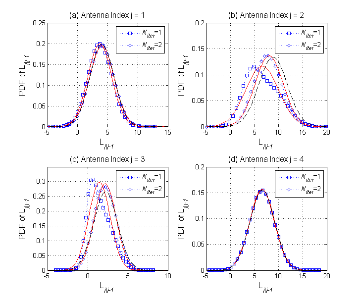
Figure 4: Density Evolution Example for N=M=4๐‘๐‘€4N=M=4. Dotted with marks: Measured from simulation result, Solid line: Estimated via DE, Dashed: Distribution under perfect cancellation. After two iterations, no changes in LLR density have been observed in all antennas. SNR = 1/ฯƒ21superscript๐œŽ21/\sigma^{2} = 6dB.

It will also be quite interesting to consider an upper bound on SINR, which is easy to obtain while gives a quite tight bound on bit error rate. Ignoring the estimation error on the previous/next variable, the upper bound is given by

ฮณjsubscript๐›พ๐‘—\displaystyle\gamma_{j} โ‰คฮณbโ€‹oโ€‹uโ€‹nโ€‹d,j=(aj|jโˆ’1,j(R)+aj|j+1,j(R))2๐”ผโ€‹(nj|jโˆ’1(R))2+๐”ผโ€‹(nj|j+1(R))2+2โ€‹ฯƒzโ€‹z,jabsentsubscript๐›พ๐‘๐‘œ๐‘ข๐‘›๐‘‘๐‘—superscriptsubscriptsuperscript๐‘Ž๐‘…conditional๐‘—๐‘—1๐‘—subscriptsuperscript๐‘Ž๐‘…conditional๐‘—๐‘—1๐‘—2๐”ผsuperscriptsubscriptsuperscript๐‘›๐‘…conditional๐‘—๐‘—12๐”ผsuperscriptsubscriptsuperscript๐‘›๐‘…conditional๐‘—๐‘—122subscript๐œŽ๐‘ง๐‘ง๐‘—\displaystyle\leq\gamma_{bound,j}=\frac{\left(a^{(R)}_{j|j-1,j}+a^{(R)}_{j|j+1,j}\right)^{2}}{{\mathbb{E}}\left(n^{(R)}_{j|j-1}\right)^{2}+{\mathbb{E}}\left(n^{(R)}_{j|j+1}\right)^{2}+2\sigma_{zz,j}} (63)

V Numerical Results

V-A Density Evolution Example

First, we test how well the analysis work for a fixed channel matrix in micro scopic point of view. The channel matrix used is shown below, which was obtained by a random generation and rounding each element below one tenth.

๐‘ฏeโ€‹x=subscript๐‘ฏ๐‘’๐‘ฅabsent\displaystyle{\boldsymbol{H}}_{ex}=
[โˆ’0.1โˆ’0.1โ€‹jโˆ’0.5โˆ’0.4โˆ’0.1โ€‹jโˆ’0.2+0.8โ€‹j+0.2โˆ’0.7โ€‹jโˆ’0.2+0.2โ€‹jโˆ’0.1+0.2โ€‹jโˆ’0.1โˆ’0.1โ€‹jโˆ’0.1โˆ’0.1โ€‹j+0.2+0.8โ€‹jโˆ’0.4โˆ’0.2โ€‹j0.4โ€‹j+0.1โˆ’0.4โ€‹jโˆ’0.4+0.2โ€‹j+0.2+0.5โ€‹j+0.2โˆ’0.3โ€‹j]matrix0.10.1๐‘—0.50.40.1๐‘—0.20.8๐‘—0.20.7๐‘—0.20.2๐‘—0.10.2๐‘—0.10.1๐‘—0.10.1๐‘—0.20.8๐‘—0.40.2๐‘—0.4๐‘—0.10.4๐‘—0.40.2๐‘—0.20.5๐‘—0.20.3๐‘—\displaystyle\begin{bmatrix}-0.1-0.1j&-0.5&-0.4-0.1j&-0.2+0.8j\\[3.00003pt] +0.2-0.7j&-0.2+0.2j&-0.1+0.2j&-0.1-0.1j\\[3.00003pt] -0.1-0.1j&+0.2+0.8j&-0.4-0.2j&0.4j\\[3.00003pt] +0.1-0.4j&-0.4+0.2j&+0.2+0.5j&+0.2-0.3j\end{bmatrix}

Using this channel, we generate pairs of random binary data and Gaussian noise vector many times. With each pair, we apply the forward-backward recursion to obtain the LLRโ€™s and measured its empirical density. When applying the algorithm, we performed the message passing in parallel fashion, i.e., all the messages, ljโˆ’1โ†’jโ€‹โˆ€jsubscript๐‘™โ†’๐‘—1๐‘—for-all๐‘—l_{j-1\to j}\;\forall j, are initialized to zero and the message passing begins at the same time for all the nodes. Although it is typical to apply forward and backward recursion sequentially, we applied it in parallel here so that we can observe the density evolution for all the nodes at the same pace.

The results are shown in Fig.4 (a) to (d), respectively, for each node, where we plotted the density of the forward message for the first two iterations. The dotted lines with marks are the measured density, the solid lines are estimated via density evolution and the dashed lines are the density with perfect cancellation, i.e., ej|jโˆ’1โ€‹(xj)=0โ€‹โˆ€jsubscript๐‘’conditional๐‘—๐‘—1subscript๐‘ฅ๐‘—0for-all๐‘—e_{j|j-1}(x_{j})=0\;\forall j such that the SINR is given by (63). In Fig.4, it can be seen that the messages produced by node 1 and 4 converge almost at the first iteration and we cannot see changing densities with more iteration. On the other hand, one can see explicit density evolution for node 2 and 3, where the densities do not look like Gaussian at the first iteration, while they become more like Gaussian after the second message update, after which we could not observe any further changes (and, hence, we did not plot them). Note also that the densities after convergence show no or a little degradation from those with perfect cancellation of the companion signal. This suggests us that the performance based on the density under the perfect cancellation might provide a tight upper bound on various performance measures.
Refer to caption

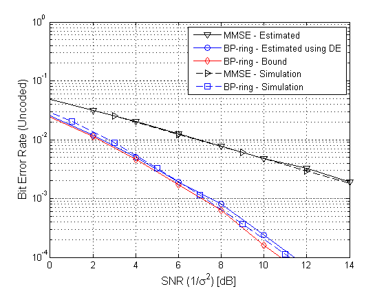
Figure 5: Uncoded bit error rate performance of MMSE receiver and BP-Ring in [13]. Solid line: Estimated, Dashed line: Simulation results.

V-B BER performance via Density evolution

To show the validity of the density evolution approach, we compare the bit error rate (BER) curves estimated using the density evolution with that obtained by simulation results without channel coding. To this end, we generated 1600 random MIMO channel matrices in the same way as did in [13] and applied density evolution to obtain the SINR of the final beliefs for each node. Using these SINRs, the BER and its bound are estimated by

PEsubscript๐‘ƒ๐ธ\displaystyle P_{E} =๐”ผ๐‘ฏโ€‹[1Mโ€‹โˆ‘j=1MQโ€‹(ฮณj)]โ‰ฅ๐”ผ๐‘ฏโ€‹[1Mโ€‹โˆ‘j=1MQโ€‹(ฮณj,bโ€‹oโ€‹uโ€‹nโ€‹d)]absentsubscript๐”ผ๐‘ฏdelimited-[]1๐‘€superscriptsubscript๐‘—1๐‘€๐‘„subscript๐›พ๐‘—subscript๐”ผ๐‘ฏdelimited-[]1๐‘€superscriptsubscript๐‘—1๐‘€๐‘„subscript๐›พ๐‘—b๐‘œ๐‘ข๐‘›๐‘‘\displaystyle={\mathbb{E}}_{\boldsymbol{H}}\left[\frac{1}{M}\sum_{j=1}^{M}Q\left(\sqrt{\gamma_{j}}\right)\right]\geq{\mathbb{E}}_{\boldsymbol{H}}\left[\frac{1}{M}\sum_{j=1}^{M}Q\left(\sqrt{\gamma_{j,{\textrm{b}ound}}}\right)\right] (64)

where ๐”ผ๐‘ฏโ€‹[โ‹…]subscript๐”ผ๐‘ฏdelimited-[]โ‹…{\mathbb{E}}_{\boldsymbol{H}}[\cdot] is the average over all channel matrices generated. We set the number of transmit and receive antenna to 4 and the number of inner iterations to 2. Fig.5 compares the BER curves obtained via density evolution and its lower bound obtained by the SINR bound in (63) with that obtained by simulation. The simulation results are the same as those in [13] without channel coding. The figure shows that (a) the BER obtained via density evolution matches perfectly to the simulation results and (b) the BER bound is quite tight showing the estimation error from the previous/next nodes has negligible effect especially for binary input. Fig.6 shows the SINR averaged over the same set of random channels, where one can see approximately 1.7 dB SINR gain over the linear MMSE receivers at low SNR region (at around 2dB SNR), which is quite good match to the result in [22].
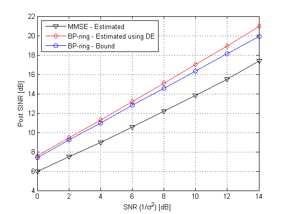
Refer to caption


Figure 6: Average SINR of MMSE receiver and BP-Ring in [13].
๐”ผโ€‹(nj|jโˆ’1(R)โ€‹nj|jโˆ’1(I))๐”ผsubscriptsuperscript๐‘›๐‘…conditional๐‘—๐‘—1subscriptsuperscript๐‘›๐ผconditional๐‘—๐‘—1\displaystyle{\mathbb{E}}\left(n^{(R)}_{j|j-1}n^{(I)}_{j|j-1}\right) =๐”ผโ€‹(โ„œโก[๐’˜jHโ€‹(๐‘ฏ{j,jโˆ’1}โ€‹๐’™{j,jโˆ’1}+๐’)]โ€‹โ„‘โก[๐’˜jHโ€‹(๐‘ฏ{j,jโˆ’1}โ€‹๐’™{j,jโˆ’1}+๐’)])absent๐”ผsuperscriptsubscript๐’˜๐‘—๐ปsubscript๐‘ฏ๐‘—๐‘—1subscript๐’™๐‘—๐‘—1๐’superscriptsubscript๐’˜๐‘—๐ปsubscript๐‘ฏ๐‘—๐‘—1subscript๐’™๐‘—๐‘—1๐’\displaystyle={\mathbb{E}}\left(\Re\left[{{\boldsymbol{w}}_{j}^{H}}({\boldsymbol{H}}_{\{j,j-1\}}{\boldsymbol{x}}_{\{j,j-1\}}+{\boldsymbol{n}})\right]\Im\left[{{\boldsymbol{w}}_{j}^{H}}({\boldsymbol{H}}_{\{j,j-1\}}{\boldsymbol{x}}_{\{j,j-1\}}+{\boldsymbol{n}})\right]\right)
=๐’˜j(R)Tโ€‹(๐‘ฏ{j,jโˆ’1}(R)โ€‹๐‘ฏ(I){j,jโˆ’1}T)โ€‹๐’˜j(R)โˆ’๐’˜j(R)Tโ€‹(๐‘ฏ{j,jโˆ’1}(R)โ€‹๐‘ฏ(R){j,jโˆ’1}T+ฯƒ22โ€‹๐‘ฐ)โ€‹๐’˜j(I)absentsuperscriptsuperscriptsubscript๐’˜๐‘—๐‘…๐‘‡subscriptsuperscript๐‘ฏ๐‘…๐‘—๐‘—1subscriptsuperscriptsuperscript๐‘ฏ๐ผ๐‘‡๐‘—๐‘—1superscriptsubscript๐’˜๐‘—๐‘…superscriptsuperscriptsubscript๐’˜๐‘—๐‘…๐‘‡subscriptsuperscript๐‘ฏ๐‘…๐‘—๐‘—1subscriptsuperscriptsuperscript๐‘ฏ๐‘…๐‘‡๐‘—๐‘—1superscript๐œŽ22๐‘ฐsuperscriptsubscript๐’˜๐‘—๐ผ\displaystyle={{\boldsymbol{w}}_{j}^{(R)}}^{T}\left({\boldsymbol{H}}^{(R)}_{\{j,j-1\}}{{{\boldsymbol{H}}^{(I)}}^{T}_{\{j,j-1\}}}\right){{\boldsymbol{w}}_{j}^{(R)}}-{{\boldsymbol{w}}_{j}^{(R)}}^{T}\left({\boldsymbol{H}}^{(R)}_{\{j,j-1\}}{{{\boldsymbol{H}}^{(R)}}^{T}_{\{j,j-1\}}}+\frac{\sigma^{2}}{2}{\boldsymbol{I}}\right){{\boldsymbol{w}}_{j}^{(I)}}
+๐’˜j(I)Tโ€‹(๐‘ฏ{j,jโˆ’1}(I)โ€‹๐‘ฏ(R){j,jโˆ’1}T)โ€‹๐’˜j(I)โˆ’๐’˜j(I)Tโ€‹(๐‘ฏ{j,jโˆ’1}(I)โ€‹๐‘ฏ(I){j,jโˆ’1}T+ฯƒ22โ€‹๐‘ฐ)โ€‹๐’˜j(R)superscriptsuperscriptsubscript๐’˜๐‘—๐ผ๐‘‡subscriptsuperscript๐‘ฏ๐ผ๐‘—๐‘—1subscriptsuperscriptsuperscript๐‘ฏ๐‘…๐‘‡๐‘—๐‘—1superscriptsubscript๐’˜๐‘—๐ผsuperscriptsuperscriptsubscript๐’˜๐‘—๐ผ๐‘‡subscriptsuperscript๐‘ฏ๐ผ๐‘—๐‘—1subscriptsuperscriptsuperscript๐‘ฏ๐ผ๐‘‡๐‘—๐‘—1superscript๐œŽ22๐‘ฐsuperscriptsubscript๐’˜๐‘—๐‘…\displaystyle+{{\boldsymbol{w}}_{j}^{(I)}}^{T}\left({\boldsymbol{H}}^{(I)}_{\{j,j-1\}}{{{\boldsymbol{H}}^{(R)}}^{T}_{\{j,j-1\}}}\right){{\boldsymbol{w}}_{j}^{(I)}}-{{\boldsymbol{w}}_{j}^{(I)}}^{T}\left({\boldsymbol{H}}^{(I)}_{\{j,j-1\}}{{{\boldsymbol{H}}^{(I)}}^{T}_{\{j,j-1\}}}+\frac{\sigma^{2}}{2}{\boldsymbol{I}}\right){{\boldsymbol{w}}_{j}^{(R)}}

VI Concluding Remarks

In this paper, we considered the convergence and density evolution of a low complexity MIMO detection based on belief propagation over ring-type pair-wise graph. The algorithm was originally proposed in [13], where utilizing the ring-type pair-wise graph the belief propagation algorithm could be expressed as a forward backward recursion and the link level performance and the convergence for Gaussian input have been analyzed. In this paper, we extended the convergence analysis to discrete alphabet. Specifically, we proved the convergence of the forward-backward recursion and devised a density evolution approach to provide an asymptotic performance in terms of average bit error rate and SINR. The BER curves shows perfect match with simulation results provided in [13], which validates the density evolution approach for binary input and the performance improvements of the algorithm in [13] over the linear MMSE receiver.

[Statistics of nj|jยฑ1(R)subscriptsuperscript๐‘›๐‘…conditional๐‘—plus-or-minus๐‘—1n^{(R)}_{j|j\pm 1} and nj|jยฑ1(I)subscriptsuperscript๐‘›๐ผconditional๐‘—plus-or-minus๐‘—1n^{(I)}_{j|j\pm 1} ]

Without loss of generality, we consider only nj|jโˆ’1(R)subscriptsuperscript๐‘›๐‘…conditional๐‘—๐‘—1n^{(R)}_{j|j-1} and nj|jโˆ’1(I)subscriptsuperscript๐‘›๐ผconditional๐‘—๐‘—1n^{(I)}_{j|j-1}. First, from the definition of nj|jโˆ’1subscript๐‘›conditional๐‘—๐‘—1n_{j|j-1} , we obtain

๐”ผโ€‹(nj|jโˆ’1(R))2๐”ผsuperscriptsubscriptsuperscript๐‘›๐‘…conditional๐‘—๐‘—12\displaystyle{\mathbb{E}}\left(n^{(R)}_{j|j-1}\right)^{2} =๐”ผโ€‹(โ„œโก[๐’˜jHโ‹…(๐‘ฏ{j,jโˆ’1}โ€‹๐’™{j,jโˆ’1}โ€‹๐’)])2absent๐”ผsuperscriptโ‹…superscriptsubscript๐’˜๐‘—๐ปsubscript๐‘ฏ๐‘—๐‘—1subscript๐’™๐‘—๐‘—1๐’2\displaystyle={\mathbb{E}}\left(\Re\left[{{\boldsymbol{w}}_{j}^{H}}\cdot({\boldsymbol{H}}_{\{j,j-1\}}{\boldsymbol{x}}_{\{j,j-1\}}{\boldsymbol{n}})\right]\right)^{2}
=๐’˜j(R)Tโ€‹(๐‘ฏ{j,jโˆ’1}(R)โ€‹๐‘ฏ(R){j,jโˆ’1}T+ฯƒ22โ€‹๐‘ฐ)โ€‹๐’˜j(R)absentsuperscriptsuperscriptsubscript๐’˜๐‘—๐‘…๐‘‡subscriptsuperscript๐‘ฏ๐‘…๐‘—๐‘—1subscriptsuperscriptsuperscript๐‘ฏ๐‘…๐‘‡๐‘—๐‘—1superscript๐œŽ22๐‘ฐsuperscriptsubscript๐’˜๐‘—๐‘…\displaystyle=\;{{\boldsymbol{w}}_{j}^{(R)}}^{T}\left({\boldsymbol{H}}^{(R)}_{\{j,j-1\}}{{{\boldsymbol{H}}^{(R)}}^{T}_{\{j,j-1\}}}+\frac{\sigma^{2}}{2}{\boldsymbol{I}}\right){{\boldsymbol{w}}_{j}^{(R)}}
+๐’˜j(R)Tโ€‹(๐‘ฏ{j,jโˆ’1}(R)โ€‹๐‘ฏ(I){j,jโˆ’1}T)โ€‹๐’˜j(I)superscriptsuperscriptsubscript๐’˜๐‘—๐‘…๐‘‡subscriptsuperscript๐‘ฏ๐‘…๐‘—๐‘—1subscriptsuperscriptsuperscript๐‘ฏ๐ผ๐‘‡๐‘—๐‘—1superscriptsubscript๐’˜๐‘—๐ผ\displaystyle+{{\boldsymbol{w}}_{j}^{(R)}}^{T}\left({\boldsymbol{H}}^{(R)}_{\{j,j-1\}}{{{\boldsymbol{H}}^{(I)}}^{T}_{\{j,j-1\}}}\right){{\boldsymbol{w}}_{j}^{(I)}}
+๐’˜j(I)Tโ€‹(๐‘ฏ{j,jโˆ’1}(I)โ€‹๐‘ฏ(R){j,jโˆ’1}T)โ€‹๐’˜j(R)superscriptsuperscriptsubscript๐’˜๐‘—๐ผ๐‘‡subscriptsuperscript๐‘ฏ๐ผ๐‘—๐‘—1subscriptsuperscriptsuperscript๐‘ฏ๐‘…๐‘‡๐‘—๐‘—1superscriptsubscript๐’˜๐‘—๐‘…\displaystyle+{{\boldsymbol{w}}_{j}^{(I)}}^{T}\left({\boldsymbol{H}}^{(I)}_{\{j,j-1\}}{{{\boldsymbol{H}}^{(R)}}^{T}_{\{j,j-1\}}}\right){{\boldsymbol{w}}_{j}^{(R)}}
+๐’˜j(I)Tโ€‹(๐‘ฏ{j,jโˆ’1}(I)โ€‹๐‘ฏ(I){j,jโˆ’1}T+ฯƒ22โ€‹๐‘ฐ)โ€‹๐’˜j(I)superscriptsuperscriptsubscript๐’˜๐‘—๐ผ๐‘‡subscriptsuperscript๐‘ฏ๐ผ๐‘—๐‘—1subscriptsuperscriptsuperscript๐‘ฏ๐ผ๐‘‡๐‘—๐‘—1superscript๐œŽ22๐‘ฐsuperscriptsubscript๐’˜๐‘—๐ผ\displaystyle+{{\boldsymbol{w}}_{j}^{(I)}}^{T}\left({\boldsymbol{H}}^{(I)}_{\{j,j-1\}}{{{\boldsymbol{H}}^{(I)}}^{T}_{\{j,j-1\}}}+\frac{\sigma^{2}}{2}{\boldsymbol{I}}\right){{\boldsymbol{w}}_{j}^{(I)}}

where we used ๐”ผโ€‹[๐’™โ€‹๐’™H]=๐‘ฐ๐”ผdelimited-[]๐’™superscript๐’™๐ป๐‘ฐ{\mathbb{E}}[{\boldsymbol{xx}}^{H}]={\boldsymbol{I}} and

๐”ผโ€‹[๐’(R)โ€‹๐’(R)T]๐”ผdelimited-[]superscript๐’๐‘…superscriptsuperscript๐’๐‘…๐‘‡\displaystyle{\mathbb{E}}\left[{\boldsymbol{n}}^{(R)}{{\boldsymbol{n}}^{(R)}}^{T}\right] =๐”ผโ€‹[๐’(R)โ€‹๐’(R)T]=ฯƒ22โ€‹๐‘ฐabsent๐”ผdelimited-[]superscript๐’๐‘…superscriptsuperscript๐’๐‘…๐‘‡superscript๐œŽ22๐‘ฐ\displaystyle={\mathbb{E}}\left[{\boldsymbol{n}}^{(R)}{{\boldsymbol{n}}^{(R)}}^{T}\right]=\frac{\sigma^{2}}{2}{\boldsymbol{I}}
๐”ผโ€‹[๐’(R)โ€‹๐’(I)T]๐”ผdelimited-[]superscript๐’๐‘…superscriptsuperscript๐’๐ผ๐‘‡\displaystyle{\mathbb{E}}\left[{\boldsymbol{n}}^{(R)}{{\boldsymbol{n}}^{(I)}}^{T}\right] =๐ŸŽabsent0\displaystyle={\boldsymbol{0}}

Note that, from independence among columns of ๐‘ฏ๐‘ฏ\boldsymbol{H} and between the real and imaginary parts, ๐’˜j(R)superscriptsubscript๐’˜๐‘—๐‘…{\boldsymbol{w}}_{j}^{(R)} and ๐’˜j(I)superscriptsubscript๐’˜๐‘—๐ผ{\boldsymbol{w}}_{j}^{(I)} are quasi-orthogonal (i.e., ๐’˜j(R)Tโ€‹๐’˜j(I)โ‰ˆ๐ŸŽsuperscriptsuperscriptsubscript๐’˜๐‘—๐‘…๐‘‡superscriptsubscript๐’˜๐‘—๐ผ0{{\boldsymbol{w}}_{j}^{(R)}}^{T}{\boldsymbol{w}}_{j}^{(I)}\approx{\boldsymbol{0}}) and, hence, the covariance is weak especially when N๐‘N is large. And, if this is the case, we can approximate

๐”ผโ€‹(nj|jโˆ’1(R))2๐”ผsuperscriptsubscriptsuperscript๐‘›๐‘…conditional๐‘—๐‘—12\displaystyle{\mathbb{E}}\left(n^{(R)}_{j|j-1}\right)^{2} โ‰ˆ๐’˜j(R)Tโ€‹(๐‘ฏ{j,jโˆ’1}(R)โ€‹๐‘ฏ(R){j,jโˆ’1}T+ฯƒ22โ€‹๐‘ฐ)โ€‹๐’˜j(R)absentsuperscriptsuperscriptsubscript๐’˜๐‘—๐‘…๐‘‡subscriptsuperscript๐‘ฏ๐‘…๐‘—๐‘—1subscriptsuperscriptsuperscript๐‘ฏ๐‘…๐‘‡๐‘—๐‘—1superscript๐œŽ22๐‘ฐsuperscriptsubscript๐’˜๐‘—๐‘…\displaystyle\approx{{\boldsymbol{w}}_{j}^{(R)}}^{T}\left({\boldsymbol{H}}^{(R)}_{\{j,j-1\}}{{{\boldsymbol{H}}^{(R)}}^{T}_{\{j,j-1\}}}+\frac{\sigma^{2}}{2}{\boldsymbol{I}}\right){{\boldsymbol{w}}_{j}^{(R)}}
+๐’˜j(I)Tโ€‹(๐‘ฏ{j,jโˆ’1}(I)โ€‹๐‘ฏ(I){j,jโˆ’1}T+ฯƒ22โ€‹๐‘ฐ)โ€‹๐’˜j(I)superscriptsuperscriptsubscript๐’˜๐‘—๐ผ๐‘‡subscriptsuperscript๐‘ฏ๐ผ๐‘—๐‘—1subscriptsuperscriptsuperscript๐‘ฏ๐ผ๐‘‡๐‘—๐‘—1superscript๐œŽ22๐‘ฐsuperscriptsubscript๐’˜๐‘—๐ผ\displaystyle+{{\boldsymbol{w}}_{j}^{(I)}}^{T}\left({\boldsymbol{H}}^{(I)}_{\{j,j-1\}}{{{\boldsymbol{H}}^{(I)}}^{T}_{\{j,j-1\}}}+\frac{\sigma^{2}}{2}{\boldsymbol{I}}\right){{\boldsymbol{w}}_{j}^{(I)}}

Similarly, we obtain

๐”ผโ€‹(nj|jโˆ’1(I))2๐”ผsuperscriptsubscriptsuperscript๐‘›๐ผconditional๐‘—๐‘—12\displaystyle{\mathbb{E}}\left(n^{(I)}_{j|j-1}\right)^{2} โ‰ˆ๐’˜j(R)Tโ€‹(๐‘ฏ{j,jโˆ’1}(I)โ€‹๐‘ฏ(I){j,jโˆ’1}T+ฯƒ22โ€‹๐‘ฐ)โ€‹๐’˜j(R)absentsuperscriptsuperscriptsubscript๐’˜๐‘—๐‘…๐‘‡subscriptsuperscript๐‘ฏ๐ผ๐‘—๐‘—1subscriptsuperscriptsuperscript๐‘ฏ๐ผ๐‘‡๐‘—๐‘—1superscript๐œŽ22๐‘ฐsuperscriptsubscript๐’˜๐‘—๐‘…\displaystyle\approx{{\boldsymbol{w}}_{j}^{(R)}}^{T}\left({\boldsymbol{H}}^{(I)}_{\{j,j-1\}}{{{\boldsymbol{H}}^{(I)}}^{T}_{\{j,j-1\}}}+\frac{\sigma^{2}}{2}{\boldsymbol{I}}\right){{\boldsymbol{w}}_{j}^{(R)}}
+๐’˜j(I)Tโ€‹(๐‘ฏ{j,jโˆ’1}(R)โ€‹๐‘ฏ(R){j,jโˆ’1}T+ฯƒ22โ€‹๐‘ฐ)โ€‹๐’˜j(I)superscriptsuperscriptsubscript๐’˜๐‘—๐ผ๐‘‡subscriptsuperscript๐‘ฏ๐‘…๐‘—๐‘—1subscriptsuperscriptsuperscript๐‘ฏ๐‘…๐‘‡๐‘—๐‘—1superscript๐œŽ22๐‘ฐsuperscriptsubscript๐’˜๐‘—๐ผ\displaystyle+{{\boldsymbol{w}}_{j}^{(I)}}^{T}\left({\boldsymbol{H}}^{(R)}_{\{j,j-1\}}{{{\boldsymbol{H}}^{(R)}}^{T}_{\{j,j-1\}}}+\frac{\sigma^{2}}{2}{\boldsymbol{I}}\right){{\boldsymbol{w}}_{j}^{(I)}}

The covariance between nj|jโˆ’1(R)subscriptsuperscript๐‘›๐‘…conditional๐‘—๐‘—1n^{(R)}_{j|j-1} and nj|jโˆ’1(I)subscriptsuperscript๐‘›๐ผconditional๐‘—๐‘—1n^{(I)}_{j|j-1} can also be obtained similar way, as shown on top of this page. From independence among columns of ๐‘ฏ๐‘ฏ\boldsymbol{H} and between the real part and imaginary part, ๐’˜j(R)Tโ€‹๐’˜j(I)โ‰ˆ๐ŸŽsuperscriptsuperscriptsubscript๐’˜๐‘—๐‘…๐‘‡superscriptsubscript๐’˜๐‘—๐ผ0{{\boldsymbol{w}}_{j}^{(R)}}^{T}{\boldsymbol{w}}_{j}^{(I)}\approx{\boldsymbol{0}} and ๐‘ฏj,jโˆ’1(R)โ€‹๐‘ฏj,jโˆ’1(I)Tโ‰ˆ๐ŸŽsuperscriptsubscript๐‘ฏ๐‘—๐‘—1๐‘…superscriptsuperscriptsubscript๐‘ฏ๐‘—๐‘—1๐ผ๐‘‡0{{\boldsymbol{H}}_{j,j-1}^{(R)}}{{\boldsymbol{H}}_{j,j-1}^{(I)}}^{T}\approx{\boldsymbol{0}}, so that the covariance is weak especially when N๐‘N is large.

References

  • [1] G.ย Caire, โ€œStatistical physics and the analysis of exact belief-propagation decoding of cdma,โ€ in Proc. JWCC, 2002, p. 30โ€“32, Barolo, Italy.
  • [2] R.ย R.ย Mรผller G.ย Caire and T.ย Tanaka, โ€œIterative multiuser joint decoding: Optimal power allocation and low-complexity implementation,โ€ IEEE Trans. Info. Th., vol. 50, pp. 1950โ€“1973, Sept. 2004.
  • [3] Y.ย Kabashima, โ€œA CDMA multiuser detection algorithm on the basis of belief propagation,โ€ J. Phys. A., pp. 11111โ€“11121, 2003.
  • [4] T.ย Tanaka and M.ย Okada, โ€œApproximate belief propagation, density evolution, and neurodynamics for CDMA multiuser detection,โ€ IEEE Trans. Info. Th., vol. 51, no. 2, pp. 700โ€“706, Feb. 2005.
  • [5] A.ย Montanari and D.ย Tse, โ€œAnalysis of belief propagation for nonlinear problems: The example of cdma (or: How to prove tanakaโ€™s formula,โ€ in Proc. of IEEE Info. Th. Workshop, Mar. 2006, pp. 122โ€“126, Punta del Este, Uruguay.
  • [6] C.-C. Wang and D.ย Guo, โ€œBelief propagation is asymptotically equivalent to map estimation for sparse linear systems,โ€ pp. 926โ€“935, Nov. 2006.
  • [7] J.ย Hu and T.ย M. Duman, โ€œGraph-based detector for BLAST architecture,โ€ in Proc. IEEE Int. Conf. on Comm., June 2007, pp. 1018โ€“1023.
  • [8] J.ย Goldberger and A.ย Leshem, โ€œMIMO decoding based on stochastic reconstruction from multiple projections,โ€ in Proc. IEEE Int. Conf. Acoust., Speech and Sig. Proc., April 2009, pp. 2457โ€“2460.
  • [9] J.ย Goldberger and A.ย Leshem, โ€œIterative tomographic solution of integer least squares problems with applications to mimo detection,โ€ IEEE JSTSP, vol. 5, no. 8, pp. 1486โ€“1496, Dec. 2011.
  • [10] M.ย Suneel, P.ย Som, A.ย Chockalingam, and B.ย S. Rajan, โ€œBelief propagation based decoding of large non-orthogonal STBCs,โ€ in Proc. IEEE Int. Symp. Info. Th., June 28โ€“July 3 2009, pp. 2003โ€“2007.
  • [11] P.ย Som, T.ย Datta, A.ย Chockalingam, and B.S. Rajan, โ€œImproved large-MIMO detection based on damped belief propagation,โ€ in Proc. of IEEE Info. Th. Workshop, Jan. 2010.
  • [12] S.ย Yoon, โ€œA low complexity mimo detection based on pairwise markov random fields,โ€ in Proc. IEEE Veh. Technol. Conf. 2011 Spring, May. 2011.
  • [13] S.ย Yoon and C.-B. Chae, โ€œLow-complexity mimo detection based on belief propagation over pairwise graphs,โ€ IEEE Trans. on Veh. Technol., vol. 63, no. 5, pp. 2363โ€“2377, June 2014.
  • [14] J.ย S. Yedidia, W.ย T. Freeman, and Y.ย Weiss, โ€œUnderstanding belief propagation and its generalizations,โ€ in Proc. Int. Joint. Conf. on Artificial Intelligence, 2001.
  • [15] J.ย S. Yedidia, W.ย T. Freeman, and Y.ย Weiss, โ€œBethe free energy, kikuchi approximations, and belief propagation algorithms,โ€ MERL Tech. Report, 2000.
  • [16] A.ย Montanari, B.ย Prabhakar, and D.ย Tse, โ€œBelief propagation based multi-user detection,โ€ in Proc. of Allerton Conf. on Comm. Control and Comp., Sep. 2005.
  • [17] D.ย Bickson, O.ย Shental, P.ย H. Siegel, J.ย K. Wolf, , and D.ย Dolev, โ€œLinear detection via belief propagation,โ€ in Proc. of Allerton Conf. on Comm. Control and Comp., Sep. 2007.
  • [18] S.ย Yoon and S.ย Lee, โ€œA detection algorithm for multi-input multi-output (MIMO) transmission using poly-diagonalization and trellis decoding,โ€ IEEE Jour. Select. Areas in Comm., vol. 26, no. 8, pp. 993โ€“1002, Aug. 2008.
  • [19] D.ย Bickson, O.ย Shental, P.ย H. Siegel, J.ย K. Wolf, and D.ย Dolev, โ€œGaussian belief propagation based multiuser detection,โ€ in Proc. IEEE Int. Symp. Info. Th., July 2008, pp. 1878โ€“1882.
  • [20] P.ย Pakzad and V.ย Anantharam, โ€œBelief propagation and statistical physics,โ€ in Proc. Conf. Inform. Sci. Sys, Mar. 2002, Princeton, NJ.
  • [21] S.ย M. Aji, G.ย B. Horn, and R.ย J. McEliece, โ€œIterative decoding on graphs with a single cycle,โ€ in Proc. IEEE Int. Symp. Info. Th., Aug. 1998, p. 276.
  • [22] J.ย Lee S.-J.ย Yoon and S.ย Yoon, โ€œPerformance of mimo detectors with a capacity-approaching code,โ€ in Proc. ICTC 2015, Nov. 2015.