The local value of in an inhomogeneous universe
Abstract
The effects of local inhomogeneities on low redshift determinations are studied by estimating the redshift-distance relation of mock sources in N-body simulations. The results are compared to those obtained using the standard approach based on Hubble’s law. The comparison shows a clear tendency for the standard approach to yield lower values of than the approach based on the scheme using light rays. The difference is, however, small. More precisely, it is found that the overall effect of inhomogeneities on the determination of is a small increase in the local estimates of about compared to the results obtained with Hubble’s law, when based on a typical distribution of supernovae in the redshift range .
The overall conclusion of the study is a verification of the results that have earlier been obtained by using Hubble’s law: The effects of inhomogeneities on local estimates are not significant enough to make it plausible that differences in high- and low-redshift estimates of are due to small inhomogeneities within the setting of standard cosmology.
1 Introduction
Overall, the CDM model is consistent with observations at a remarkable level considering the model’s simplicity compared to the real, inhomogeneous universe. However, some observational inconsistencies do exist when observations are interpreted within the Friedmann-Lemaitre-Robertson-Walker (FLRW) regime. One such inconsistency is differences in the Hubble constant when determined by different types of observations. In particular, CMB and BAO observations, pertaining to the large scale universe, yield smaller values of than local observations such as those based on supernova redshift-distance relations [1, 2, 3]. As pointed out in e.g. [4], the different estimates are not actually inconsistent and might for instance simply be due to systematic effects not properly accounted for. Nevertheless, the tension between the different values of is conspicuous and deserves to be studied further.
Observations are primarily interpreted using FLRW predictions. The Universe is, however, not an FLRW universe at an exact level and the spatial inhomogeneities and anisotropies of the real universe may affect especially low-redshift observations and their interpretation. Inhomogeneities may in principle also affect large-scale observations such as those of the CMB. The general expectation is that this is not the case though – an expectation supported by the studies in e.g. [5, 6, 7] (see however also111Note that it is also in [9] concluded that an inhomogeneous spacetime can have significant effects on estimates based on CMB observations. The conclusion is however based on an erroneous analysis which is later corrected by the same authors in [5].
[8]). This implies that the tension between the different estimates may be a result of small scale inhomogeneities primarily affecting the low-redshift estimates while the large scale estimates of can be considered yielding the global value. In order to investigate whether or not this is the case, quantitative theoretical considerations regarding low-redshift estimates of are needed. Several different types of studies of effects of inhomogeneities have been conducted, mostly either based on perturbation theory (e.g. [10, 11, 12, 13, 14, 15]) or swiss-cheese and onion models (e.g. [17, 16, 18, 19, 20, 21, 22, 23, 24, 25, 26]). The results from such studies are not always consistent with each other and are hence not conclusive at this point, although there is a tendency for the studies to indicate a negligible effect of inhomogeneities on observations after averaging over many observed sources (unless there is significant backreaction [27, 28, 18]). However, studies of effects of inhomogeneities only seldom focus on low-redshift determinations. One of the few studies focused on low-redshift estimates was presented in [29] where it was shown that spatial inhomogeneities may affect estimates at an observationally significant level. In contrast to this, studies based on Newtonian N-body simulations indicate that local inhomogeneities do not significantly affect local estimates and thus that local inhomogeneities cannot explain the tension between local and global determinations of [30, 31, 32]. A crucial point with the studies based on Newtonian N-body simulations is that they are usually based on Hubble’s law. Real astrophysical observations are based on light rays that have traveled through the inhomogeneous universe to reach us. These light rays are affected by inhomogeneities in terms of e.g. the actual null-paths, their redshift, and their ray-bundle magnification. In the study presented here, such effects are taken into account when computing redshift-distance relations in Newtonian N-body simulations. The resulting redshift-distance data points are fitted to the background FLRW relation with as the fitting parameter. If the discrepancy between the different types of determinations is due to one type (CMB + BAO) probing the global value while the other (low-redshift) studies yield a local value affected by inhomogeneities, then the best-fit value obtained here should be larger than the N-body background value of .
2 Method for computing redshift-distance relations in N-body simulations at low redshift
In order to study the effects of inhomogeneities on the local measurement of , mock observations are constructed by computing redshift-distance data points using results from an N-body simulation. The formalism for computing redshift-distance data points is introduced below while practical aspects regarding the N-body simulation are described in section 3.
A recipe for going between Newtonian N-body simulations and a relativistic spacetime corresponding to the first order perturbed FLRW metric in the Newtonian gauge was given in [33]. By using N-body data based on exact, inhomogeneous solutions to Einstein’s equations, it was in [34, 35] shown that the recipe leads to a very precise reproduction of redshift-distance relations in an inhomogeneous universe as long as the anisotropy of the individual structures is low. The particular procedure for computing redshift-distance relations studied in [35] will be used here. The study in [35] only included mildly non-linear structures, but in relation to the study presented here, a similar precision of the method has been confirmed for density fractions in the range , where is the density of the assumed “background”. (The precision of the method for inhomogeneities outside this range has not been studied.) The procedure is therefore expected to yield fairly accurate estimates of redshift-distance relations including effects of inhomogeneities.
The procedure is only summarized below, and the reader is referred to e.g. [33, 35] or the other references cited in this section for elaborations.
The observed redshift of a light ray with tangent vector is computed following the standard definition . The subscripts and indicate evaluation at the spacetime position of observation and emission respectively such that e.g. is the observer velocity and is the velocity of the source. The velocity field is given by , where are the velocity components obtained from the N-body simulation and the normalization factor is computed according to the findings of [35].
The effects of inhomogeneities on the angular diameter distance can be described by the convergence such that the angular diameter distance along light rays in the N-body simulation is given by . denotes the angular diameter distance at according to the FLRW background of the N-body simulation. Once the angular diameter distance is known, the corresponding luminosity distance can be computed using the distance duality relation .
At linear level, the convergence is divided into several different contributions including the (integrated) Sachs-Wolfe contributions, a gravitational contribution and a Doppler contribution. In general, the two dominant contributions are the gravitational convergence and the Doppler convergence. As shown in [36, 37, 35], the gravitational contribution to the convergence is, however, irrelevant at low redshifts. Hence, for the purpose of the current study, the angular diameter distance can be computed as , where denotes the Doppler convergence. The Doppler convergence can be computed by (see e.g. [38]):
| (2.1) |
where denotes conformal time and is the (spatial) velocity of the source. The Einstein convention is used with running over the spatial indices . The vector is the propagation direction unit -vector, i.e. . It is sufficient to use the background version of and in that case is the unit vector pointing in the direction from the source to the observer.
In the expression for the Doppler convergence given above, a term due to the peculiar motion of the observer has been omitted. This is justified by noting that the observer velocity can be estimated by measuring the CMB dipole and hence has no consequences when interpreting real observations. Note also that in equation (2.1), the scale factor etc. are evaluated at the spacetime position corresponding to the observed redshift , not a background redshift computed with the background metric.
When mock redshift-distance data points have been obtained as described above, they are fitted to the expression for the luminosity distance in an FLRW universe,
| (2.2) |
When fitting, is used as fitting parameter while and are fixed to the values used in the N-body simulation.
Before moving on, it should be noted that the Doppler convergence occurs because of the difference between the observed redshift and the redshift obtained from background computations (see e.g. [36, 37, 14, 38, 39]). The effects of inhomogeneities studied here are therefore effects of peculiar velocities. The peculiar velocities are gravitationally induced by an inhomogeneous energy density and the effects of the peculiar velocities are thus effects of having a spacetime that deviates from the exactly spatially homogeneous and isotropic FLRW spacetimes. This fact will in the following be emphasized by referring to an “inhomogeneous velocity field” instead of “peculiar velocities”.
Note lastly, that the effects of an inhomogeneous velocity field on e.g. local estimates was also studied in [40], where it was argued that the effects can actually be understood without invoking general relativity.
3 Mock observations
This section serves to introduce the construction of the mock observations used for the study. The (mock) observations are based on a Newtonian N-body simulation with cosmological parameters in agreement with the 2013 results from the Planck collaboration [1], i.e. the cosmological parameters are set according to and (. The simulation is performed using a modified version of the GADGET-2 code [41], with initial conditions generated using a code written by J. Brandbyge [42] based on transfer functions computed using CAMB222http://camb.info/ [43]. The simulation is run in a box of side length , containing dark matter particles. The simulation is initiated at a redshift of and run until present time.
Box size, simulation resolution and source distribution on the sky will not be varied here as it was in [32] shown that such variations have only small effects on the results.
Velocities and positions of sources as well as positions of observers are obtained by identifying these with halos, which are found using the halo-finder ROCKSTAR [44].
As seen in equation (2.1), the velocity fields of the sources are highly important for computing the Doppler convergence. It was demonstrated in [17] that the effects of inhomogeneities on observations will depend on the smoothing scales used to obtain e.g. the velocity field from the discrete N-body data. This issue is here overcome by estimating source velocities as the velocities of bound structures, i.e. halos, in the simulation. Assuming that galaxies follow the motion of their dark matter host halos, this procedure corresponds to probing the velocity field in the same manner as is done in real observations.
3.1 Redshift distribution of sources
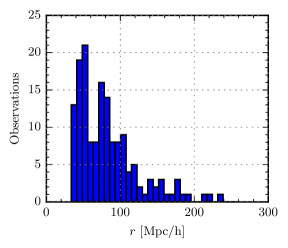
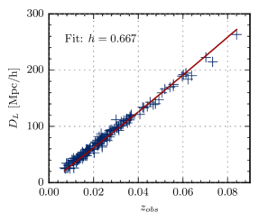
The redshift distribution of the sources affects the study; the further away the sources are, the less impact the peculiar velocities have. To understand the significance of the sources’ redshift distribution, two different redshift distribution schemes are used. In one of the schemes, the sources are distributed according to the redshift distribution of the 155 supernovae of the CfA3+OLD sample [46, 45].
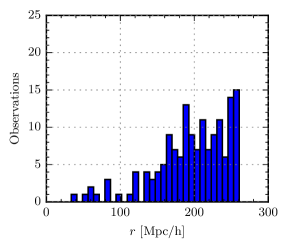
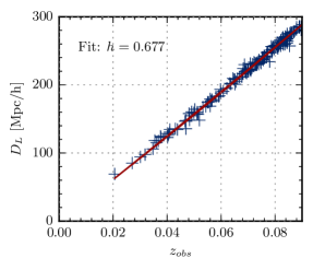
The other scheme selects the 155 sources according to a mass weighted distribution, in which each halo in the distance range is selected with a probability proportional to its mass333This distribution scheme builds on the assumption that the probability of a type Ia supernova occurring in a given halo is proportional to the halo mass. However, as seen in figure 1, the scheme leads to a redshift distribution which is significantly different than the distribution of the CfA3+OLD sample.. This distribution has the advantage that it is growing as a function of distance (due to the increasing volume of shells). Using this distribution scheme thereby provides a check that the estimates converge to the true value at large distances. Note also that it is this second scheme that was used in [32].
The difference between the two types of distributions is illustrated in figure 1. The figure also shows an example of the differences in estimates based on observations following the two schemes.
3.2 Observers
In order to take cosmic variance into account444The term “cosmic variance” is here used to mean the uncertainty in observations due to our ability to only observe the Universe from a single spacetime position., each set of mock observations are based on a group of observers instead of a single observer. The observer positions are still important for the study as the local environment may bias observations at low and intermediate redshifts. For instance, placing the observers in massive halos amounts to placing them in infall regions and will thus lead to a bias of peculiar source velocities, and hence redshifts, in the direction towards the observer which will again lead to a smaller estimate. This is predicted by gravitational instability theory [47, Chapter 5], and can in principle be corrected for by subtracting the peculiar motion induced by the local density field when analyzing real observational data (see e.g. [48]). Such a correction was for instance made in [3].
In order to study the effects of the local environment of the observers, two different sets of observers are used. The first set consists of observers residing in subhalos of mass in a host halo in the mass range . This approximately corresponds to our position in the Local Group galaxy cluster, a member of the Virgo Super Cluster. The second set of observers are placed at random positions throughout the simulation volume. As underdense regions take up the larger part of the volume, these observers will tend to be positioned in underdense regions.
When observers are placed in halos, their peculiar velocities are taken to be those of the host halos. When they are placed at random positions, they are assumed to be at rest with respect to the background. The observer velocities enter into the computations of the observed redshift and so using these two different methods for estimating observer velocities may affect the results. This has been tested not to be the case though; setting the observer velocities to zero in the case where the observers are placed in halos is insignificant for the results.
3.3 Lightcone snapshots
The velocity in equation (2.1) is the comoving velocity of the source at the time of emission. The mock observations are carried out in the halo catalog at . However, comoving source positions change over time due to the sources’ peculiar velocities (which also change over time). Since the study made here is based on low-redshift observations with , this cosmic evolution should not affect the results at a significant level. To test this assessment, two types of halo catalogs are made. One is based on a regular GADGET-2 snapshot at , while the other type is based on lightcone snapshots555The lightcone snapshots are created by using a plug-in to GADGET-2 written by Troels Haugbølle. The same plug-in was used in [32]. (one for each observer). ROCKSTAR’s lightcone functionality can be used for identifying structures in such a snapshot. In the resulting halo catalog, the positions and velocities are stored as they were at the time of emission.
3.4 Summary
In figure 2, an example of the observations performed by a single observer is shown. As seen, the observers view the full sky. See e.g. [32] for the effects of using smaller sky coverage.
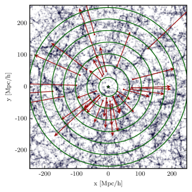
Following the various schemes discussed above, a number of different analyses have been performed. These are summarized in
table 1.
Since the lightcone snapshots are very time consuming to use, only a single analysis is made with these. That analysis is denoted Dlc and is the analysis which best resembles real observations.
| Figure | Analysis name | Observer positions | SN-distribution | Fit | Lightcone |
|---|---|---|---|---|---|
| Dref | Subhalos | Typical | Full | No | |
| 3 | Href | Subhalos | Typical | Linear | No |
| Dlc | Subhalos | Typical | Full | Yes | |
| Dmw | Subhalos | Mass Weighted | Full | No | |
| 4 | Drp | Random Positions | Typical | Full | No |
| Hrp | Random Positions | Typical | Linear | No | |
| Hmw | Subhalos | Mass Weighted | Linear | No |
4 Results and discussion
Figures 3 and 4 show how the local estimates of are distributed among the observers in the different analyses. Specifically, the deviation in the local Hubble constant from the true value, , is shown as a function of the distance to the most distant bin included in the estimate of . The sources are distributed in bins according to their comoving distances from the observer, which are related to the redshifts of the FLRW background via .
The mean value of the deviation is shown with a solid line, and the 68.3%, 95.4% and 99.7% confidence intervals are indicated with either shaded areas or dashed lines.
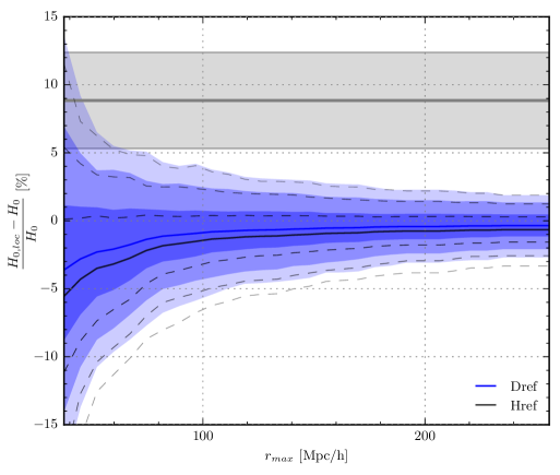
The results are shown using different combinations of choices for the observer positions, redshift distribution of supernovae, and fitting method. An overview of the different combinations that have been studied is given in table 1 where a naming scheme for the analyses is also introduced. Analysis Dlc is the analysis which is closest to actual observations; it uses observers placed in subhalos with a typical supernova distribution in a lightcone snapshot and obtains by a fit to the FLRW redshift-distance relation as explained in section 3. In figure 4, analysis Dlc is compared to analysis Dref which differs from Dlc only in that it is based on a regular GADGET-2 snapshot. As seen, the difference between using the two types of snapshots is negligible.
Figure 3 compares analysis Dref to analysis Href. Analysis Href differs from analysis Dref in that has been obtained using Hubble’s law. The comparison shows that the mean estimate is smaller when Hubble’s law is used instead of the recipe based on the Doppler convergence as described in section 2. The difference is quite small, ranging from 1.9% in the innermost bin to 0.3% in the outermost bin. A similar result is seen in figure 4, i.e. the analyses based on Hubble’s law consistently yield a estimate that is slightly smaller than the estimate of the corresponding analysis based on the Doppler convergence computations described in section 2.
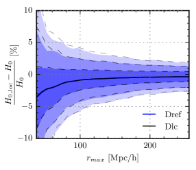
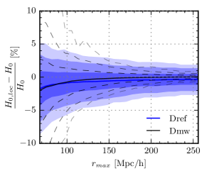
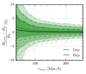
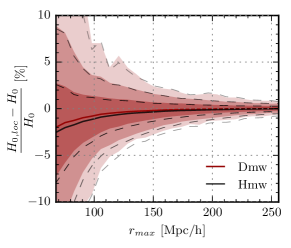
Figure 4 illustrates the importance of using realistic source and observer distributions. In particular, the figure shows that by changing the observer positions to be random, the estimates grow. This is because underdense regions take up more of the simulation volume and hence will be favored when using random observer positions. The result can thus be considered a type of Hubble-bubble effect (see e.g. [49, 50, 51, 52, 53, 54, 55]). This type of Hubble-bubble result is particularly interesting since there in fact are some indications that we may be living in an underdense region of the Universe [56, 57, 58].
The figure also shows that the distribution of sources has impact on especially the uncertainty of the estimates. Specifically, the spread in the results is much less when higher-redshift sources are favored in the observations. This is consistent with peculiar motions being less important at larger distances.
Lastly, it is noted that the results presented here yield mean estimates that are lower than the value of the N-body background. The only exception to this result is the analyses with random observer positions discussed above. Within the standard cosmological scheme studied here, the effect of peculiar velocity fields thus seems to be to reduce the local value of compared to the global value. Hence, inhomogeneities cannot provide a solution to the tension of different types of estimates. In fact, the results show that inhomogeneities will in principle increase the tension. As mentioned in section 3.2, to the extent that the shift in the mean estimate of compared to the global value is a result of the local environment at the observer position, this can be corrected for when interpreting real observations.
5 Summary
N-body simulations were used to study low-redshift determinations of in an inhomogeneous universe. In particular, it was studied whether or not an inhomogeneous velocity field leads to a local value different from the global value, the latter corresponding to that of the N-body background and which is what one expects to measure using high-redshift observations such as those based on the CMB. The values were obtained by approximating light paths according to the background model and computing the angular diameter distance of objects by using the Doppler convergence to take effects of inhomogeneities into account. Inhomogeneities were also taken into account when computing source redshifts. This procedure differs from that used in earlier work of this kind, where determinations have been estimated by using the linear relation known as Hubble’s law. The results obtained with the method introduced here consistently lead to a mean value which is higher than that obtained by simply using Hubble’s law. The difference is, however, very small.
The estimates were found to be slightly lower than the background value except in a single of the studied cases: When the observers are placed at random positions in the simulation box, the resulting mean estimate is slightly above that of the N-body background. This result is similar to the Hubble-bubble effect.
As source distances and numbers are increased, all the estimates converge towards the value of of the N-body background.
The results summarized above indicate that the tension between high- and low-redshift determinations of cannot be alleviated by taking inhomogeneities into account – at least not without straying from standard cosmology.
6 Acknowledgments
We thank the anonymous referee for suggestions that have significantly improved the presentation of the work.
Parts of the numerical work for this project have been done using computer resources from the Center for Scientific Computing Aarhus.
References
- [1] Planck Collaboration: Planck 2013 results. I. Overview of products and scientific results, A&A 571, A1 (2014), arXiv:1303.5062v2 [astro-ph.CO]
- [2] Wendy L. Freedman et al.: Carnegie Hubble Program: A Mid-Infrared Calibration of the Hubble Constant, 2012, ApJ, 758, 24
- [3] Adam G. Riess et al.: A 3% Solution: Determination of the Hubble Constant with the Hubble Space Telescope and Wide Field Camera 3, ApJ,730,119, 2011, arXiv:1103.2976v1 [astro-ph.CO]
- [4] George Efstathiou: Revisited, MNRAS 440, 1138–1152 (2014), arXiv:1311.3461v2 [astro-ph.CO]
- [5] Camille Bonvin, Chris Clarkson, Ruth Durrer, Roy Maartens, Obinna Umeh: Do we care about the distance to the CMB? Clarifying the impact of second-order lensing, arXiv:1503.07831v1
- [6] Nick Kaiser, John A. Peacock: On the Bias of the Distance-Redshift Relation from Gravitational Lensing, arXiv:1503.08506 [astro-ph.CO]
- [7] Mikko Lavinto, Syksy Rasanen: CMB seen through random Swiss Cheese, JCAP10(2015)057, arXiv:1507.06590v3 [astro-ph.CO]
- [8] Krzysztof Bolejko: The effect of inhomogeneities on the distance to the last scattering surface and the accuracy of the CMB analysis, JCAP 02(2011)025, arXiv:1101.3338v1
- [9] Chris Clarkson, Obinna Umeh, Roy Maartens, Ruth Durrer: What is the distance to the CMB?, JCAP 1411 (2014) 11, 036, arXiv:1405.7860v3 [astro-ph.CO]
- [10] Obinna Umeh, Chris Clarkson, Roy Maartens: Nonlinear relativistic corrections to cosmological distances, redshift and gravitational lensing magnification. I - Key results, Class. Quantum Grav. 31 202001, arXiv:1207.2109v3 [astro-ph.CO]
- [11] Ido Ben-Dayan, Giovanni Marozzi, Fabien Nugier, Gabriele Veneziano: The second-order luminosity-redshift relation in a generic inhomogeneous cosmology, JCAP 1211 (2012) 045, arXiv:1209.4326v2 [astro-ph.CO]
- [12] I. Ben-Dayan, M. Gasperini, G. Marozzi, F. Nugier, G. Veneziano: Average and dispersion of the luminosity-redshift relation in the concordance model, 10.1088/1475-7516/2013/06/002, arXiv:1302.0740v3 [astro-ph.CO]
- [13] Enea Di Dio, Ruth Durrer: Vector and Tensor Contributions to the Luminosity Distance, Phys. Rev. D 86, 023510 (2012), arXiv:1205.3366v3 [astro-ph.CO]
- [14] Camille Bonvin, Ruth Durrer, M. Alice Gasparini: Fluctuations of the luminosity distance, Phys.Rev.D73:023523,2006, arXiv:astro-ph/0511183v5
- [15] Chris Clarkson, Kishore Ananda, Julien Larena: The influence of structure formation on the cosmic expansion, Phys.Rev.D80:083525,2009, Phys.Rev.D80:083525,2009
- [16] Pierre Fleury, Helene Dupuy, Jean-Philippe Uzan: Can all cosmological observations be accurately interpreted with a unique geometry?, Phys. Rev. Lett. 111, 091302 (2013), arXiv:1304.7791v2 [astro-ph.CO]
- [17] Timothy Clifton, Joe Zuntz: Hubble Diagram Dispersion From Large-Scale Structure, Mon. Not. R. Astron. Soc. 400 (2009) 2185, arXiv:0902.0726v2 [astro-ph.CO]
- [18] Mikko Lavinto, Syksy Rasanen, Sebastian J. Szybka: Average expansion rate and light propagation in a cosmological Tardis spacetime, JCAP12(2013)051, arXiv:1308.6731v2 [astro-ph.CO]
- [19] Valerio Marra, Edward W. Kolb, Sabino Matarrese: Light-cone averages in a swiss-cheese universe, Phys.Rev.D77:023003,2008, arXiv:0710.5505v2 [astro-ph]
- [20] Valerio Marra, Edward W. Kolb, Sabino Matarrese, Antonio Riotto: On cosmological observables in a swiss-cheese universe, Phys.Rev.D76:123004, 2007, arXiv:0708.3622v3 [astro-ph]
- [21] Krzysztof Bolejko: The Szekeres Swiss Cheese model and the CMB observations, Gen.Rel.Grav.41:1737-1755, 2009, arXiv:0804.1846v2 [astro-ph]
- [22] Sebastian J. Szybka: On light propagation in Swiss-Cheese cosmologies, Phys.Rev.D84:044011, 2011, arXiv:1012.5239v2 [astro-ph.CO]
- [23] Sima Ghassemi, Salomeh Khoeini Moghaddam, Reza Mansouri: Lensing effects in inhomogeneous cosmological models, Phys.Rev.D79:102002, 2009, arXiv:0901.0340v1 [astro-ph.CO]
- [24] Austin Peel, M. A. Troxel, Mustapha Ishak: Effect of inhomogeneities on high precision measurements of cosmological distances, Phys. Rev. D 90, 123536 (2014), arXiv:1408.4390v2 [astro-ph.CO]
- [25] Pierre Fleury, Hélène Dupuy, Jean-Philippe Uzan: Interpretation of the Hubble diagram in a nonhomogeneous universe, Physical Review D 87, 123526 (2013), arXiv:1302.5308v2 [astro-ph.CO]
- [26] Nikolai Meures, Marco Bruni: Redshift and distances in a CDM cosmology with non-linear inhomogeneities, 2012, MNRAS 419, 3, 1937, arXiv:1107.4433v2 [astro-ph.CO]
- [27] Syksy Rasanen: Light propagation in statistically homogeneous and isotropic universes with general matter content, JCAP 1003:018,2010, arXiv:0912.3370v2 [astro-ph.CO]
- [28] Syksy Rasanen: Light propagation in statistically homogeneous and isotropic dust universes, JCAP 0902:011,2009,
- [29] Ido Ben-Dayan, Ruth Durrer, Giovanni Marozzi, Dominik J. Schwarz: The value of in the inhomogeneous Universe, Phys. Rev. Lett. 112, 221301 (2014) , arXiv:1401.7973v3 [astro-ph.CO]
- [30] R. Wojtak, A. Knebe, W. A. Watson, I. T. Iliev, S. Heß, D. Rapetti, G. Yepes and S. Gottlöber: Cosmic variance of the local Hubble flow in large-scale cosmological simulations, Mon. Not. Roy. Astron. Soc. 438 (2014) 2, 1805, arXiv:1312.0276v2 [astro-ph.CO]
- [31] Xiangdong Shi, Michael S. Turner: Expectations for the Difference Between Local and Global Measurements of the Hubble Constant, Astrophys.J. 493 (1998) 519, arXiv:astro-ph/9707101v2
- [32] Io Odderskov, Steen Hannestad, Troels Haugbølle: On the local variation of the Hubble constant, JCAP10(2014)028, arXiv:1407.7364v2 [astro-ph.CO]
- [33] Stephen R. Green and Robert M. Wald: Newtonian and Relativistic Cosmologies, Phys.Rev.D85:063512, (2012)
- [34] S. M. Koksbang, S. Hannestad: Methods for studying the accuracy of light propagation in N-body simulations, Phys. Rev. D 91, 043508 (2015), arXiv:1501.01413v2 [astro-ph.CO]
-
[35]
S. M. Koksbang, S. Hannestad: Studying the precision of ray tracing techniques with Szekeres models, arXiv:1506.09127v1 [astro-ph.CO]
See also S. M. Koksbang, S. Hannestad: Erratum: Studying the precision of ray tracing techniques with Szekeres models [Phys. Rev. D 92, 023532 (2015)], Phys. Rev. D 92, 069904 (2015) - [36] Krzysztof Bolejko, Chris Clarkson, Roy Maartens, David Bacon, Nikolai Meures, Emma Beynon: Anti-lensing: the bright side of voids, Phys. Rev. Lett. 110, 021302 (2013), arXiv:1209.3142v3 [astro-ph.CO]
- [37] David J. Bacon, Sambatra Andrianomena, Chris Clarkson, Krzysztof Bolejko, Roy Maartens: Cosmology with Doppler Lensing, MNRAS 443 (2014) 1900-1915 , arXiv:1401.3694v2 [astro-ph.CO]
- [38] Camille Bonvin: Effect of Peculiar Motion in Weak Lensing, Phys.Rev.D78:123530, 2008,arXiv:0810.0180v3 [astro-ph]
- [39] Lam Hui, Patrick B. Greene: Correlated Fluctuations in Luminosity Distance and the (Surprising) Importance of Peculiar Motion in Supernova Surveys, Phys. Rev. D 73 (2006) 123526, [astro-ph/0512159].
- [40] N. Kaiser and M. J. Hudson: Kinematic Bias in Cosmological Distance Measurement, Mon. Not. Roy. Astron. Soc. 454 (2015) 1, 280 [arXiv:1502.01762 [astro-ph.CO]].
- [41] V. Springel: The Cosmological simulation code GADGET-2, Mon. Not. Roy. Astron. Soc. 364 (2005) 1105 [astro-ph/0505010].
- [42] J. Brandbyge: Quantitative Cosmology - Massive Neutrinoes in non-linear Structure Formation, PhD. thesis, Aarhus University, Denmark, 2010
- [43] A. Lewis and S. Bridle: Cosmological parameters from CMB and other data: A Monte Carlo approach, Phys. Rev. D 66 (2002) 103511, [astro-ph/0205436]
- [44] Behroozi, P. S., Wechsler, R. H., Wu, H.-Y.: The ROCKSTAR Phase-space Temporal Halo Finder and the Velocity Offsets of Cluster Cores, [arxiv:1110.4372]
- [45] M. Hicken, P. Challis, S. Jha, R. P. Kirsher, T. Matheson et al: CfA3: 185 Type Ia Supernova Light Curves from the CfA, Astrophys. J. 700 (2009), arXiv:astro-ph/0901.4787
- [46] S. Jha, A. G. Riess and R. P. Kirshner: Improved Distances to Type Ia Supernovae with Multicolor Light Curve Shapes: MLCS2k2, Astrophys. J. 659 (2007) 122, [astro-ph/0612666]
- [47] Phillip James Edwin Peebles: Principles of Physical Cosmology, Princeton University Press (1993)
- [48] SNLS collaboration, James D. Neill, Michael J. Hudson, and Alex Conley: The Peculiar Velocities of Local Type Ia Supernovae and their Impact on Cosmology, Astrophys. J. 661 (2007) L123, [arxiv:0704.1654]
- [49] Valerio Marra, Luca Amendola, Ignacy Sawicki, Wessel Valkenburg: Cosmic variance and the measurement of the local Hubble parameter, Phys. Rev. Lett. 110, 241305 (2013), arXiv:1303.3121v4
- [50] Y. Suto, T. Suginohara, Y. Inagaki: Limits on the global Hubble constant and the age of the universe, Prog.Theor.Phys. 93 (1995) 839-844, arXiv:astro-ph/9412090v1
- [51] Idit Zehavi, Adam G. Riess, Robert P. Kirshner, Avishai Dekel: A Local Hubble Bubble from Type Ia Supernovae?, Astrophys.J. 503 (1998) 483, arXiv:astro-ph/9802252v2
- [52] R. Giovanelli, Daniel Dale, Martha Haynes, Eduardo Hardy, Luis Campusano: No Hubble Bubble in the Local Universe, ApJ 525 25 (1999), arXiv:astro-ph/9906362v1
- [53] Xiangdong Shi, Lawrence M. Widrow, L. Jonathan Dursi: Measuring Hubble’s Constant in our Inhomogeneous Universe, arXiv:astro-ph/9506120v1
- [54] Kiyotomo Ichiki, Chul-Moon Yoo, Masamune Oguri: Relationship between the CMB, SZ Cluster Counts, and Local Hubble Parameter Measurements in a Simple Void Model, arXiv:1509.04342v2 [astro-ph.CO]
- [55] Saurabh Jha, Adam G. Riess, Robert P. Kirshner: Improved Distances to Type Ia Supernovae with Multicolor Light Curve Shapes: MLCS2k2, Astrophys.J.659:122-148,2007, arXiv:astro-ph/0612666v1
- [56] R. C. Keenan, A. J. Barger and L. L. Cowie: Evidence for a 300 megaparsec scale under-density in the local galaxy distribution, 2013, ApJ, 775, 62
- [57] R. C. Keenan, A. J. Barger, L. L. Cowie, W.-H. Wang, I. Wold, and L. Trouille: Testing for a large local void by investigating the near-infrared galaxy luminosity function, 2012, ApJ, 754, 131
- [58] R. C. Keenan, L. Trouille, A. J. Barger, L. L. Cowie, and W.-H. Wang: An extremely deep, wide-field near-infrared survey: bright galaxy counts and local large scale structure, 2010, ApJS, 186, 94