Detecting Deviating Data Cells

Abstract

A multivariate dataset consists of $n$ cases in $d$ dimensions, and is often stored in an $n$ by $d$ data matrix. It is well-known that real data may contain outliers. Depending on the situation, outliers may be (a) undesirable errors which can adversely affect the data analysis, or (b) valuable nuggets of unexpected information. In statistics and data analysis the word outlier usually refers to a row of the data matrix, and the methods to detect such outliers only work when at least half the rows are clean. But often many rows have a few contaminated cell values, which may not be visible by looking at each variable (column) separately. We propose the first method to detect deviating data cells in a multivariate sample which takes the correlations between the variables into account. It has no restriction on the number of clean rows, and can deal with high dimensions. Other advantages are that it provides predicted values of the outlying cells, while imputing missing values at the same time. We illustrate the method on several real data sets, where it uncovers more structure than found by purely columnwise methods or purely rowwise methods. The proposed method can help to diagnose why a certain row is outlying, e.g. in process control. It also serves as an initial step for estimating multivariate location and scatter matrices.

Keywords: Cellwise outlier, Missing values, Multivariate data, Robust estimation, Rowwise outlier.

1 INTRODUCTION

Most data sets come in the form of a rectangular matrix $\boldsymbol{X}$ with $n$ rows and $d$ columns, where $n$ is called the sample size and $d$ the dimension. The rows of $\boldsymbol{X}$ correspond to the cases, whereas the columns are the variables. Both $n$ and $d$ can be large, and it may happen that $d>n$. There exist many data models as well as techniques to fit them, such as regression and principal component analysis.

It is well-known that many data sets contain outliers. Depending on the circumstances, outliers may be (a) undesirable errors which can adversely affect the data analysis, or (b) valuable nuggets of unexpected information. Either way, it is important to be able to detect the outliers, which can be hard for high $d$.

In statistics and data analysis the word outlier typically refers to a row of the data matrix, as in the left panel of Figure 1. There has been much research since the 1960’s to develop fitting methods that are less sensitive to such outlying rows, and that can detect the outliers by their large residual (or distance) from that fit. This topic goes by the name of robust statistics, see e.g. the books by Maronna et al. (2006) and Rousseeuw and Leroy (1987).

Recently researchers have come to realize that the outlying rows paradigm is no longer sufficient for modern high-dimensional data sets. It often happens that most data cells (entries) in a row are regular and just a few of them are anomalous. The first paper to formulate the cellwise paradigm was (Alqallaf et al., 2009). They noted how outliers propagate: given a fraction $\varepsilon$ of contaminated cells at random positions, the expected fraction of contaminated rows is

$$1-(1-\varepsilon)^{d}$$ (1)

which quickly exceeds 50% for increasing $\varepsilon$ and/or increasing dimension $d$, as illustrated in the right panel of Figure 1. This is fatal because rowwise methods cannot handle more than 50% of contaminated rows if one assumes some basic invariance properties, see e.g. (Lopuhaä and Rousseeuw, 1991).

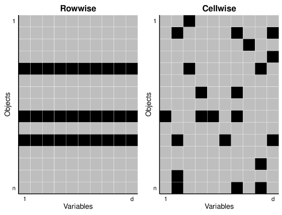
Figure 1: The rowwise and cellwise outlier paradigms (black means outlying).

The two paradigms are quite different. The outlying row paradigm is about cases that do not belong in the dataset, for instance because they are members of a different population. Its basic units are the cases, and if you interpret them as points in $d$-dimensional space they are indeed indivisible. But if you consider a case as a row in a matrix then it can be divided, into cells. The cellwise paradigm assumes that some of these cells deviate from the values they should have had, perhaps due to gross measurement errors, whereas the remaining cells in the same row still contain useful information.

The anomalous data cells problem has proved to be quite hard, as the existing tools do not suffice. Recent progress was made by Danilov (2010),  Van Aelst et al. (2012), Agostinelli et al. (2015),  Öllerer et al. (2016), and Leung et al. (2016).

Figure 2: Illustration of bivariate outliers.

Note that in the right panel of Figure 1 we do not know at the outset which (if any) cells are black (outlying), in stark contrast with the missing data framework. To illustrate the difficulty of detecting deviating data cells let us look at the artificial bivariate ($d=2$) example in Figure 2. Case 1 lies within the near-linear pattern of the majority, whereas cases 2, 3, and 4 are outliers. The first coordinate of case 2 lies among the majority of the $x_{i1}$ (depicted as tickmarks under the horizontal axis) while its second coordinate $x_{22}$ is an outlying cell. For case 3, the first cell $x_{31}$ is outlying. But what about case 4? Both of its coordinates fall in the appropriate ranges. Either coordinate of case 4 could be responsible for the point standing out, so the problem is not identifiable. We would have to flag the entire row 4 as outlying.

But now suppose that we obtain five more variables (columns) for these cases, which are correlated with the columns we already have. Then it may be possible to see that $x_{41}$ perfectly agrees with the values in the new cells of row 4, whereas $x_{42}$ does not. Then we would conclude that the cell $x_{42}$ is the culprit. Therefore, this is one of the rare situations where a higher dimensionality is not a curse but can be turned into an advantage. In fact, the method proposed in the next section typically performs better when the number of dimensions increases.

This example shows that deviating data cells do not need to stand out in their column: it suffices that they disobey the pattern of relations between this variable and those correlated with it. Here we propose the first method for detecting deviating data cells that takes the correlations between the variables into account. Unlike existing methods, our DetectDeviatingCells (DDC) method is not restricted to data with over 50% of clean rows. Other advantages are that it can deal with high dimensions and that it provides predicted values of the outlying cells. As a byproduct it imputes missing values in the data. For software availability see Section 8.

2 BRIEF SKETCH OF THE METHOD

The (possibly idealized) model states that the rows $\boldsymbol{x}_{i}$ were generated from a multivariate Gaussian distribution with unknown $d$-variate mean $\boldsymbol{\mu}$ and positive semidefinite covariance matrix $\boldsymbol{\Sigma}$, after which some cells were corrupted or became missing. However, the algorithm will still run if the underlying distribution is not multivariate Gaussian.

The method uses various devices from robust statistics and is described more fully in Section 4. We only sketch the main ideas here. The method starts by standardizing the data and flagging the cells that stand out in their column. Next, each data cell is predicted based on the unflagged cells in the same row whose column is correlated with the column in question. Finally, a cell for which the observed value differs much from its predicted value is considered anomalous. The method then produces an imputed data matrix, which is like the original one except that cellwise outliers and missing values are replaced by their predicted values. The method can also flag an entire row if it contains too much anomalous behavior, so that we have the option of downweighting or dropping that row in subsequent fits to the data.

This method looks unusual but it successfully navigates around the many pitfalls inherent in the problem, and worked the best out of the many approaches we tried. Its main feature is the prediction of individual cells. This can be characterized as a locally linear fit, where ‘locally’ is not meant in the usual sense (of Euclidean distance) but instead refers to the space of variables endowed with a kind of correlation-based metric.

Along the way DDC imputes missing data values by their predicted values. This is far less efficient than the EM algorithm of Dempster et al. (1977) when the data are Gaussian and outlier-free, but it is more robust against cellwise outliers.

The DDC method has the natural equivariance properties. If we add a constant to all the values in a column of $X$, or multiply any column by a nonzero factor, or reorder the rows or the columns, the result will change as expected.

3 EXAMPLES

The first dataset was scraped from the website of the British television show Top Gear by Alfons (2016). It contains 11 objectively measured numerical variables about 297 cars. Five of these variables (such as Price) were rather skewed so we logarithmically transformed them.

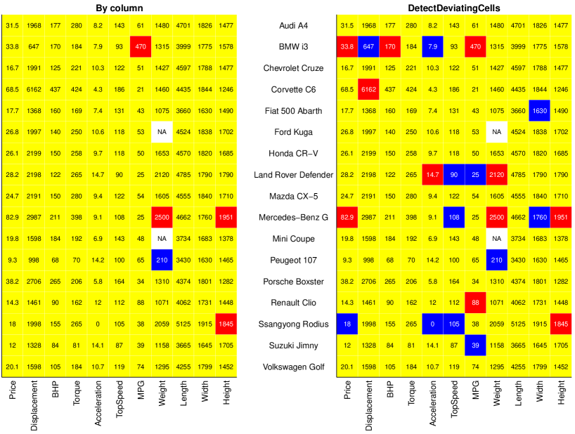
Figure 3: Selected rows from cell maps of Top Gear data: (left) when detecting anomalous data cells per column; (right) when using the proposed method.

The left panel of Figure 3 shows the result of applying a simple univariate outlier identifier to each of the columns of this dataset separately. For column $j$ this method first computes a robust location $m_{j}$ (such as the median) of its values, as well as a robust scale $s_{j}$ and then computes the standardized values $z_{ij}=(x_{ij}-m_{j})/s_{j}$. A cell is then flagged as outlying if $|z_{ij}|>c$ where the cutoff $c=2.576$ corresponds to a tolerance of 99% so that under ideal circumstances about 1% of the cells would be flagged. Most of the cells were yellow, indicating they were not flagged. Here we only show some of the more interesting rows out of the 297. Deviating cells whose $z_{ij}$ is positive are colored red, and those with negative $z_{ij}$ are in blue. Missing data are shown in white and labeled NA (from ‘Not Available’).

The right hand panel of Figure 3 shows the corresponding cell map obtained by running DetectDeviatingCells on these data. In the algorithm we used the same 99% tolerance setting yielding the same cutoff $c=2.576$. The color of the deviating cells now reflects whether the observed cell value is much higher or much lower than the predicted cell value.

The new method shows much more structure than looking by column only. The high gas mileage (MPG) of the BMW i3 is no longer the only thing that stands out, and in fact it is an electric vehicle with a small additional gas engine. The columnwise method does not flag the Corvette’s displacement which is not that unusual by itself, but it is high in relation to the car’s other characteristics. None of the properties of the Land Rover Defender (an all-terrain vehicle) stand out on their own, but their combination does. The weight of 210 kg listed for the Peugeot 107 is clearly an error, which gets picked up by both methods. The univariate method only flags the height of the Ssangyong Rodius, whereas DetectDeviatingCells also notices that its acceleration time of zero seconds from 0 to 62 mph is too low compared to its other properties, and in fact it is physically impossible.

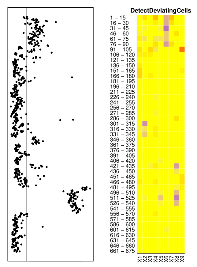
Figure 4: Left: robust distances of the rows of the Philips data. Right: map of DetectDeviatingCells on these data, combined per blocks of 15 rows.

As a second example we take the Philips dataset which measures $d=9$ characteristics of $n=677$ TV parts created by a new production line. The left panel of Figure 4 is a rotated version of Figure 9(a) in (Rousseeuw and Van Driessen, 1999) and shows, from top to bottom, the robust distance $RD_{i}$ for $i=1,\ldots,n$. These were computed as

$$\mbox{RD}_{i}=\sqrt{(\boldsymbol{x}_{i}-\boldsymbol{T})^{\prime}\boldsymbol{S}^{-1}(\boldsymbol{x}_{i}-\boldsymbol{T})}$$

where $\boldsymbol{T}$ and $\boldsymbol{S}$ are the estimates of location and scatter obtained by the Minimum Covariance Determinant (MCD) from (Rousseeuw, 1985), a rowwise robust method. It shows that the process was out of control in the beginning (roughly rows 1–90) and near the end (around rows 480–550). However, by itself this does not yet tell us what happened in those products.

In the right panel we see the cell map of DDC. The analysis was carried out on all 677 rows, but in order to display the results we created blocks of 15 rows and 1 column. The color of each cell is the ‘average color’ over the block. The resulting cell map indicates that in the beginning variable 6 had lower values than would be predicted from the remaining variables, whereas the later outliers were linked with lower values of variable 8. (In between, the cell map gives hints about some more isolated deviations.) We do not claim that this is the complete answer, but at least it gives an initial indication of what to look for. (DDC also flagged some rows, but this is not shown in the cell map to avoid confusion.) Note that these data are not literally a multivariate sample because the rows were provided consecutively, but both the MCD and DDC methods ignore the time order of the rows.

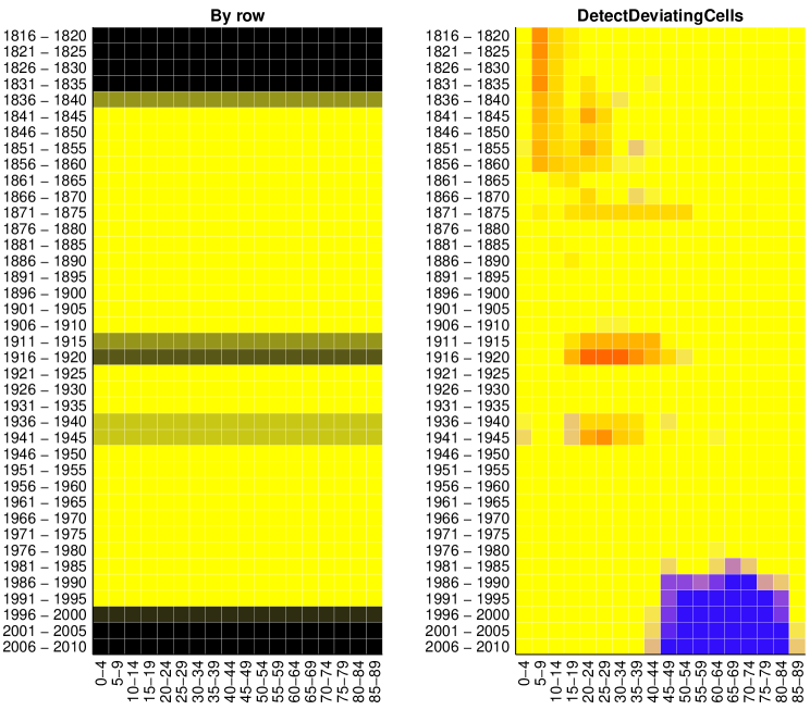
Figure 5: Male mortality in France in 1816–2010: (left) detecting outlying rows by a robust PCA method; (right) detecting outlying cells by DetectDeviatingCells. After the analysis, the cells were grouped in blocks of $5\times 5$ for visibility.

The next example is the mortality by age for males in France, from 1816 to 2010 as obtained from the Human Mortality Database (2015). An earlier version was analyzed by Hyndman and Shang (2010). Each case corresponds to the mortalities in a given year. The left panel in Figure 5 was obtained by ROBPCA (Hubert et al., 2005), a rowwise robust method for principal component analysis. Such a method can only detect entire rows, and the rows it has flagged are represented as black horizontal lines. A black row doesn’t reveal any information about its cells. The analysis was carried out on the data set with the individual years and the individual ages, but as this resolution would be too high to fit on the page we have combined the cells into $5\times 5$ blocks afterward. The combination of some black rows with some yellow ones has led to gray blocks. We can see that there were outlying rows in the early years, the most recent years, and during two periods in between.

By contrast, the right panel in Figure 5 identifies a lot more information. The outlying early years saw a high infant mortality. During the Prussian war and both world wars there was a higher mortality among young adult men. And in recent years mortality among middle-aged and older men has decreased substantially, perhaps due to medical advances.

Our final example consists of spectra with $d=750$ wavelengths collected on $n=180$ archeological glass samples (Lemberge et al., 2000). Here the number of dimensions (columns) exceeds the number of cases (rows). DetectDeviatingCells has no problems with this, and the R implementation took about 1 minute on a laptop with Intel i7-4800MQ 2.7GHz processor for this dataset. The top panel in Figure 6 shows the rows detected by the robust principal components method. The lower panel is the cell map obtained by DetectDeviatingCells on this $180\times 750$ dataset. After the analysis, the cells were again grouped in $5\times 5$ blocks. We now see clearly which parts of each spectrum are higher/lower than predicted. The wavelengths of these deviating cells reveal the chemical elements responsible.

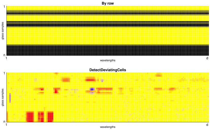
Figure 6: Cell maps of $n=180$ archeological glass spectra with $d=750$ wavelengths. The positions of the deviating data cells reveal the chemical contaminants.

In general, the result of DetectDeviatingCells can be used in several ways:

1. Ideally, the user looks at the deviating cells and whether their values are higher or lower than predicted, and makes sense of what is going on. This may lead to a better understanding of the data pattern, to changes in the way the data are collected/measured, to dropping certain rows or columns, to transforming variables, to changing the model, and so on.

2. If the data set is too large for visual inspection of the results or the analysis is automated, the deviating cells can be set to missing after which the data set is analyzed by a method appropriate for incomplete data.

3. If no such method is available, one can analyze the imputed data set $\boldsymbol{X}_{imp}$ produced by DetectDeviatingCells which has no missings.

In 2. and 3. one has the option to drop the flagged rows before taking the step. If that step is carried out by a sparse method such as the Lasso (Tibshirani, 1996; Städler et al., 2014) or another form of variable selection, one would of course look more closely at the deviating cells in the variables that were selected.

Remark. In the above examples the cellwise outliers happened to be mainly concentrated in fewer than half of the rows, allowing the rowwise robust methods MCD and ROBPCA to detect most of those rows. This may give the false impression that it would suffice to apply a rowwise robust method and then to analyze the flagged rows further. But this is not true in general: by (1) there will typically be too many contaminated rows, so rowwise robust methods will fail.

4 DETAILED DESCRIPTION OF THE ALGORITHM

The DetectDeviatingCells (DDC) algorithm has been implemented in R and Matlab (see Section 8). As described before, the underlying model is that the data are generated from a multivariate Gaussian distribution $N(\boldsymbol{\mu},\boldsymbol{\Sigma})$ but afterward some cells were corrupted or omitted. The variables (columns) of the data should thus be numerical and take on more than a few values. Therefore the code does some preprocessing: it identifies the columns that do not satisfy this condition, such as binary dummy variables, and performs its computations on the remaining columns.

These remaining variables should then be approximately Gaussian in their center, that is, apart from any outlying values. This could be verified by QQ plots, and one could flag highly skewed or long-tailed variables. It is recommended to transform very non-gaussian variables to approximate gaussianity, like we took the logarithm of the right-skewed variable Price in the cars data in Section 3. More general tools are the Box-Cox and Yeo-Johnson (Yeo and Johnson, 2000) transformations, that have parameters which need to be estimated as done by Bini and Bertacci (2006) and Riani (2008). We chose not to automate this step because we feel it is best carried out by a person with subject matter knowledge about the data. From here onward we will assume that the variables are approximately Gaussian in their center. The algorithm does not require joint normality of variables in order to run.

The actual algorithm then proceeds in eight steps.

Step 1: standardization. For each column $j$ of $\boldsymbol{X}$ we estimate

$$m_{j}=robLoc_{i}(x_{ij})\quad\mbox{ and }\quad s_{j}=robScale_{i}(x_{ij}-m_{j})$$ (2)

where robLoc is a robust estimator of location, and robScale is a robust estimator of scale which assumes its argument has already been centered. The actual definitions of these estimators are given in the Appendix. Next, we standardize $\boldsymbol{X}$ to $\boldsymbol{Z}$ by

$$z_{ij}=(x_{ij}-m_{j})/s_{j}\;\;.$$ (3)

Step 2: apply univariate outlier detection to all variables. After the columnwise standardization in (3) we define a new matrix $\boldsymbol{U}$ with entries

$$u_{ij}=\left\{\begin{array}[]{ll}z_{ij}&\text{ if }|z_{ij}|\leqslant c\\ \text{NA}&\text{ if }|z_{ij}|>c\;\;.\\ \end{array}\right.$$ (4)

Due to the standardization in (3), formula (4) is a columnwise outlier detector. The cutoff value $c$ is taken as

$$c=\sqrt{\chi^{2}_{1,p}}$$ (5)

where $\chi^{2}_{1,p}$ is the $p$-th quantile of the chi-squared distribution with 1 degree of freedom, where the probability $p$ is 99% by default so that under ideal circumstances only 1% of the entries gets flagged.

Step 3: bivariate relations. For any two variables $h\neq j$ we compute their correlation as

$$\mbox{cor}_{jh}=robCorr_{i}(u_{ij},u_{ih})$$ (6)

where robCorr is a robust correlation measure given in the Appendix (the computation is over all $i$ for which neither $u_{ij}$ or $u_{ih}$ is NA). From here onward we will only use the relation between variables $j$ and $h$ when

$$|\mbox{cor}_{jh}|\geqslant corrlim$$ (7)

in which corrlim is set to 0.5 by default. Variables $j$ that satisfy (7) for some $h\neq j$ will be called connected, and contain useful information about each other. The others are called standalone variables. For the pairs $(j,h)$ satisfying (7) we also compute

$$b_{jh}=robSlope_{i}(u_{ij}|u_{ih})$$ (8)

where robSlope computes the slope of a robust regression line without intercept that predicts variable $j$ from variable $h$ (see Appendix). These slopes will be used in the next step to provide predictions for connected variables.

Step 4: predicted values. Next we compute predicted values $\hat{z}_{ij}$ for all cells. For each variable $j$ we consider the set $H_{j}$ consisting of all variables $h$ satisfying (7), including $j$ itself. For all $i=1,\ldots,n$ we then set

$$\hat{z}_{ij}=G(\{b_{jh}u_{ih}\;;\;h\mbox{ in}\;\;H_{j}\})$$ (9)

where $G$ is a combination rule applied to these numbers, which omits the NA values and is zero when no values remain. (The latter corresponds to predicting the unstandardized cell by the estimated location of its column, which is a fail-safe.) Our current preference for $G$ is a weighted mean with weights $w_{jh}=|cor_{jh}|$ but other choices are possible, such as a weighted median. The advantage of (9) is that the contribution of an outlying cell $z_{ih}$ to $\hat{z}_{ij}$ is limited because $|u_{ih}|\leqslant c$ and it can only affect a single term, which would not be true for a prediction from a least squares multiple regression of $z_{.j}$ on the $d-1$ remaining variables $z_{.h}$ together. We will illustrate the accuracy of the predicted cells by simulation in Section 5.

Step 5: deshrinkage. Note that a prediction such as (9) tends to shrink the scale of the entries, which is undesirable. We could try to shrink less in the individual terms $b_{jh}u_{ih}$ but this would not suffice because these terms can have different signs for different $h$. Therefore, we propose to deal with the shrinkage after applying the combination rule (9). For this purpose we replace $\hat{z}_{ij}$ by $a_{j}\hat{z}_{ij}$ for all $i$ and $j$, where

$$a_{j}:=robSlope_{i^{\prime}}(z_{i^{\prime}j}|\hat{z}_{i^{\prime}j})$$ (10)

comes from regressing the observed $z_{.j}$ on the (shrunk) predicted $\hat{z}_{.j}$ .

Step 6: flagging cellwise outliers. In steps 4 and 5 we have computed predicted values $\hat{z}_{ij}$ for all cells. Next we compute the standardized cell residuals

$$r_{ij}=\frac{z_{ij}-\hat{z}_{ij}}{robScale_{i^{\prime}}(z_{i^{\prime}j}-\hat{z}_{i^{\prime}j})}\;\;.$$ (11)

In each column $j$ we then flag all cells with $|r_{ij}|>c$ as anomalous, where $c$ was given in (5). We also assemble the ‘imputed’ matrix $\boldsymbol{Z}_{imp}$ which equals $\boldsymbol{Z}$ except that it replaces deviating cells $z_{ij}$ and NA’s by their predicted values $\hat{z}_{ij}$. The unflagged cells remain as they were.

We have the option of setting the flagged cells to NA and repeating steps 4 to 6 in order to improve the accuracy of the estimates. This can be iterated.

Step 7: flagging rowwise outliers. In order to decide whether to flag row $i$ we could just count the number of cells whose $|r_{ij}|$ exceeds a cutoff $a$, but this would miss rows with many fairly large $|r_{ij}|\;<\;a$ . The other extreme would be to compare $\mathop{\mbox{ave}}_{j}(r_{ij}^{2})$ to a cutoff, but then a row with one very outlying cell would be flagged as outlying, which would defeat the purpose. We do something in between. Under the null hypothesis of multivariate Gaussian data without any outliers, the distribution of the $r_{ij}$ is close to standard Gaussian, so the cdf of $r_{ij}^{2}$ is approximately the cdf $F$ of $\chi^{2}_{1}$. This leads us to the criterion

$$T_{i}=\mathop{\mbox{ave}}_{j=1}^{d}F(r_{ij}^{2})\;\;.$$ (12)

We then standardize the $T_{i}$ as in (3) and flag the rows $i$ for which the standardized $T_{i}$ exceed the cutoff $c$ of (5).

When we find that row $i$ has an unusually large $T_{i}$ this does not necessarily ‘prove’ that it corresponds to a member of a different population, but at least it is worth looking into.

Even though the $T_{i}$ can flag some rowwise outliers, there are types of rowwise outliers that it may not detect, for instance in the barrow wheel configuration of Stahel and Mächler (2009) where a rowwise outlier may not have any large $r_{ij}^{2}$. Therefore, it is recommended to use rowwise robust methods in subsequent analyses of the data, after dropping the rows that were flagged.

Step 8: destandardize. Next, we turn the imputed matrix $\boldsymbol{Z}_{imp}$ into an imputed matrix $\boldsymbol{X}_{imp}$ by undoing the standardization in (3). The main output of DDC is $\boldsymbol{X}_{imp}$ together with the list of cells flagged as outlying and, optionally, the list of rowwise outliers that were found.

Predicting the value of a cell in steps 4 and 5 above evokes the imputation of a missing value, as in the EM algorithm of Dempster et al. (1977). However, there are two reasons why the EM method may not work in the present situation. First of all, we would need estimators of location and scatter $\hat{\boldsymbol{\mu}}$ and $\hat{\boldsymbol{\Sigma}}$ that are robust against cellwise and rowwise outliers, which we only know how to obtain after detecting those outliers. And secondly, the conditional expectation of $x_{ij}$ is a linear combination of all the available $x_{ih}$ with $h\neq j$ but some of those cells may be outlying themselves, thus spoiling the sum.

The DDC method employs measures of bivariate correlation, and regression for bivariate data. This may seem naive compared to estimating scatter matrices and/or performing multiple regression on sets of $q>2$ variables. However, the latter would imply that we must compute scatter matrices between $q$ variables in an environment where a fraction $\varepsilon$ of cells is contaminated, so that according to (1) a fraction $1-(1-\varepsilon)^{q}$ of the rows of length $q$ is expected to be contaminated. The latter fraction grows very quickly with $q$, and once it exceeds 50% there is no hope of estimating the scatter matrix by a rowwise robust method. So the larger $q$ is, the less this approach can work. Therefore we chose the smallest possible value $q=2$, which has the additional advantage that the computational effort to robustly estimate bivariate scatter is much lower than for higher $q$.

To illustrate this, Table 1 shows the effect of fitting substructures in dimension $q<d$ for various values of $q$. The total time complexity is the product of the time needed for a 50%-rowwise-breakdown fit (regression or scatter) to a $q$-variate data set (in which elemental sets are formed by $q-1$ data points and the origin) and the number of combinations of $q$ out of $d$ variables (for large $d$). The complexity grows very fast with $q$. The next column is the expected breakdown value, i.e. what fraction of evenly distributed cellwise outliers these fits can typically withstand, i.e. $1-2^{-1/q}$. The expected breakdown value drops quickly with $q$. The final column is the probability that a subrow of $q$ entries contains no outliers when the probability of a cell being outlying is 10%. Table 1 is in fact overly optimistic because it does not account for the problem that the predictions from such $q$-variate fits are affected whenever at least one of the cells in it is outlying.

Table 1: Fitting substructures in $q<d$ dimensions

	total time	breakdown	probability of
$q$	complexity	value	clean $q$-row∗
2	$n\,d\,log(d)$	29.3%	81.0%
3	$n^{2}d^{3}$	20.6%	72.9%
4	$n^{3}d^{4}$	15.9%	65.6%
5	$n^{4}d^{5}$	12.9%	59.0%
10	$n^{9}d^{10}$	6.7%	34.9%
20	$n^{19}d^{20}$	3.4%	12.2%

^∗ Assuming a 10% probability of a cell being outlying.

This should not be confused with the approach of Kriegel et al. (2009) who look for rowwise outliers under the assumption that outlyingness of a row is due to only a few variables whereas the other variables are deemed irrelevant. That situation is different from both the general rowwise outlier setting and the cellwise outlier model, in each of which all variables may be relevant.

As described, the computation time (number of operations) of DDC is on the order of $O(nd^{2})$ due to computing all $d(d-1)/2$ correlations between variables, where each correlation takes $O(n)$ time. The required memory (storage) space is then also $O(nd^{2})$. However, if the dimension $d$ is over (say) 1000 we switch to predicting each column by the $k$ columns that are most correlated with it, thereby bringing down the space requirement to $O(nd)$ which cannot be reduced further as it is proportional to the size of the data matrix itself. On a parallel architecture we can reduce the computation time by letting each processor compute the $k$ correlations for a subset of columns to be predicted. On a non-parallel system we could switch to a fast approximate $k$-nearest neighbor method such as the celebrated algorithm of Arya et al. (1999) which would lower the computation time from $O(nd^{2})$ to $O(nd\,log(d))$. Compared to analyzing each column separately, this algorithm only spends an additional time factor $log(d)$ which grows very slowly with $d$. A related speedup is used in Google Correlate (Vanderkam et al., 2013).

5 COMPARISON TO OTHER DETECTION METHODS

We now compare DDC to a method that detects outlying cells per column, the univariate GY filter of Gervini and Yohai (2002) as described in(Agostinelli et al., 2015). Applying the univariate GY filter to the columns of the cars data actually gives the same result as the simpler columnwise detection in Figure 3. The key difference between these methods is that the GY filter uses an adaptive cutoff rather than the fixed cutoff (5).

We will only report a small part of our simulations, the results of other settings being similar. First, clean multivariate Gaussian data were generated with $\boldsymbol{\mu}=\boldsymbol{0}$ and two types of covariance matrices $\boldsymbol{\Sigma}$ with unit diagonal. The ALYZ (Agostinelli et al., 2015) random correlation matrices yield relatively low correlations between the variables, whereas the A09 correlation matrix given by $\rho_{jh}=(-0.9)^{|h-j|}$ yields both high and low correlations.

Next, these clean data were contaminated. Outlying cells were generated by replacing a random subset (say, 10%) of the $n\times d$ cells by a value $\gamma$ which was varied to see its effect.

Outlying rows were generated in the hardest direction, that of the last eigenvector $\boldsymbol{v}$ of the true covariance matrix $\boldsymbol{\Sigma}$. Next we rescale $\boldsymbol{v}$ to the typical size of a data point, by making $\;\boldsymbol{v}^{\prime}{\boldsymbol{\Sigma}}^{-1}\boldsymbol{v}=E[Y^{2}]=d\;$ where $\;Y^{2}\sim\chi^{2}_{d}\;$. We then replaced a random set of rows of $\boldsymbol{X}$ by $\gamma\boldsymbol{v}$.

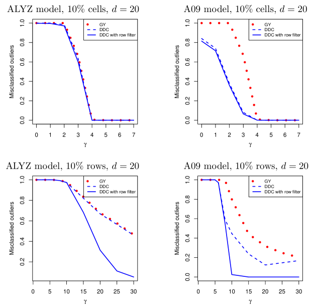
Figure 7: Outlier misclassification rates of different detection methods: (top) under cellwise contamination, (bottom) under rowwise contamination. Here GY is the Gervini-Yohai filter.

Figure 7 shows the outlier misclassification rate (for $n=200$ and $d=20$). This is the number of cells that were generated as outlying and detected by the method, divided by the total number of outlying cells generated. This fraction depends on $\gamma$: it is high for small $\gamma$ (but those cells or rows are not really outlying) and then goes down. In the top panels we see that all methods for detecting cells work about equally well when the correlations between variables are fairly small, whereas the new method does better when there are at least some higher correlations. The bottom panels show a similar effect for detecting rows, and indicate that using the row filter, i.e. step 7 in Section 4, is an important component of DDC.

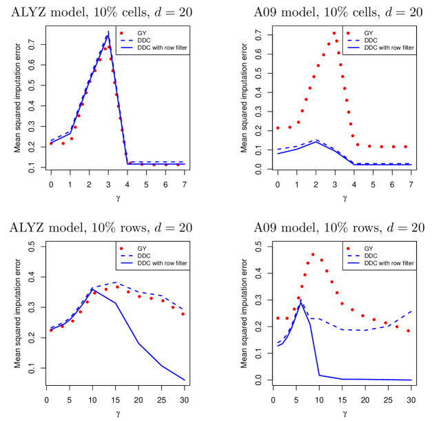
Figure 8: Mean squared error of the imputed cells in the same simulation.

The same simulation yields Figure 8, which shows the mean squared error of the imputed cells relative to the original cell values (before any contamination took place), in which flagged rows were taken out. Again DDC does best when there are some higher correlations. This confirms the usefulness of computing predicted cells in step 4 of the DDC algorithm.

We have repeated the simulations leading to Figures 7 and 8 for dimensions $d$ ranging upto 200, $n$ between 10 and 2000, and contamination fractions upto 20%, each time with 50 replications. The method does not suffer from high dimensions, and even for $n=20$ cases in $d=200$ dimensions the comparisons between these methods yield qualitatively the same conclusions.

6 TWO-STEP METHODS FOR LOCATION AND SCATTER

Now assume that we are interested in estimating the parameters of the multivariate Gaussian distribution $N(\boldsymbol{\mu},\boldsymbol{\Sigma})$ from which the data were generated (before cells and/or rows were contaminated).

If the data were clean one would estimate $\boldsymbol{\mu}$ and $\boldsymbol{\Sigma}$ by the mean of the data and the classical covariance matrix. However, when the data may contain both cellwise and rowwise outliers the problem becomes much more difficult. For this Agostinelli et al. (2015) proposed a two-step procedure called 2SGS which is the current best method. The first step applies the univariate GY filter (from the previous section) to each column of the data matrix $\boldsymbol{X}$ and sets the flagged cells to NA. The second step then applies the sophisticated Generalized S-Estimator (GSE) of Danilov et al. (2012) to this incomplete data set, yielding $\hat{\boldsymbol{\mu}}$ and $\hat{\boldsymbol{\Sigma}}$ . The GSE is a rowwise robust estimator of $\boldsymbol{\mu}$ and $\boldsymbol{\Sigma}$ that was designed to work with data containing missing values, following earlier work by Little (1988) and Cheng and Victoria-Feser (2002).

Our version of this is to replace GY in the first step by DDC, followed by the same second step. When the first step flags a row we take it out of the subsequent computations. We also include the Huberized Stahel-Donoho (HSD) estimator of Van Aelst et al. (2012), as well as the Minimum Covariance Determinant (MCD) estimator (Rousseeuw, 1985; Rousseeuw and Van Driessen, 1999) which is robust to rowwise outliers but not to cellwise outliers. For each method we measure how far $\hat{\boldsymbol{\Sigma}}$ is from the true $\boldsymbol{\Sigma}$ by the likelihood ratio type deviation

$$\mbox{LRT}=\mbox{trace}(\hat{\boldsymbol{\Sigma}}\boldsymbol{\Sigma}^{-1})-\mbox{log}(\mbox{det}(\hat{\boldsymbol{\Sigma}}\boldsymbol{\Sigma}^{-1}))-d$$

(which is a special case of the Kullback-Leibler divergence) and average this quantity over all replications.

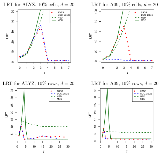
Figure 9: LRT deviation of three estimates from the true scatter matrix.

Figure 9 compares these methods in the same simulation settings as Figures 7 and 8. In the top panels we see that the new method performs about as well as 2SGS when the correlations between the variables are fairly low, but does much better when there are some higher correlations. For rowwise outliers their performance is quite similar.

Agostinelli et al. (2015) showed that 2SGS is consistent, that is, it gets the right answer for data generated from the model without any contamination when $n$ goes to infinity. The proof follows from the fact that the fraction of cells flagged by the univariate GY filter goes to zero in that setting. This is not true for DDC because the cutoff value (5) is fixed, so some cells will still be flagged. Nevertheless the above simulations indicate that with actual contamination, using DDC in the first step often does better than GY.

A limitation of the GSE in the second step is that it requires $n>d$ and in fact the dimension $d$ should not be above 20 or 30, whereas the raw DDC method can deal with higher dimensions as we saw in the glass example with $d=750$.

7 CONCLUSIONS AND OUTLOOK

The proposed method detects outliers at the level of the individual cells (entries) of the data matrix, unlike existing outlier detection methods which consider the rows (cases) of that matrix as the basic units. Its main construct is the prediction of each cell. This turns a high dimensionality into a blessing instead of a curse, as having more variables (columns) available increases the amount of information and may improve the accuracy of the predicted cells.

The new method requires more computation than considering each variable in isolation, but on the other hand is able to detect outliers that would otherwise remain hidden as we saw in the first example. In simulations we saw that DetectDeviatingCells performs as well as columnwise outlier detection when there is little correlation between the columns, whereas it does much better when there are higher correlations. Also, using it as the first step in the method of Agostinelli et al. (2015) outperforms a columnwise start.

A topic for further research is to extend this work to non-numeric variables, such as binary and nominal. For the interaction between numeric and non-numeric variables, and between non-numeric variables, this necessitates replacing correlation by other measures of bivariate association. Also, for predicting cells the linear regression would need to be replaced by other techniques such as logistic regression.

8 SOFTWARE AVAILABILITY

The R code of the DetectDeviatingCells algorithm is available on CRAN in the package cellWise, which also contains functions for drawing cell maps and allows to reproduce all the examples in this paper. Equivalent MATLAB code is available from the website http://wis.kuleuven.be/stat/robust/software .

APPENDIX

The building blocks of DetectDeviatingCells are some simple existing robust methods for univariate and bivariate data. Several are available, and our choice was based on a combination of robustness and computational efficiency, as all four of them only require $O(n)$ computing time and memory.

For estimating location and scale of a single data column we use the first step of an algorithm for M-estimators, as described on pages 39–41 of (Maronna et al., 2006). In particular, for estimating location we employ Tukey’s biweight function

$$W(t)=\left(1-\left(\frac{t}{c}\right)^{2}\right)^{2}\;I(|t|\leqslant c)$$

where $c>0$ is a tuning constant (by default $c=3$). Given a univariate dataset $Y=\{y_{1},\ldots,y_{n}\}$ we start from the initial estimates

$$m_{1}=\mathop{\mbox{med}}_{i=1}^{n}(y_{i})\quad\mbox{ and }\quad s_{1}=\mathop{\mbox{med}}_{i=1}^{n}\,|y_{i}-m_{1}|$$

and then compute the location estimate

$$robLoc(Y)=\left(\sum_{i=1}^{n}w_{i}y_{i}\right)/\left(\sum_{i=1}^{n}w_{i}\right)$$

where the weights are given by $w_{i}=W((y_{i}-m_{1})/s_{1})$ .

For estimating scale we assume that $Y$ has already been centered, e.g. by subtracting $robLoc(Y)$, so that we only need to consider deviations from zero. We now use the function $\rho(t)=\mbox{min}(t^{2},b^{2})$ where $b=2.5$. Starting from the initial estimate $s_{2}=\mathop{\mbox{med}}_{i}(|y_{i}|)$ we then compute the scale estimate

$$robScale(Y)=s_{2}\sqrt{\frac{1}{\delta}\;\mathop{\mbox{ave}}_{i=1}^{n}\rho\left(\frac{y_{i}}{s_{2}}\right)}$$

where the constant $\delta=0.845$ ensures consistency for Gaussian data.

The next methods are bivariate, i.e. they operate on two data columns, call them $j$ and $h$. For correlation we start from the initial estimate

$$\hat{\rho}_{jh}=\left((robScale_{i}(z_{ij}+z_{ih}))^{2}-(robScale_{i}(z_{ij}-z_{ih}))^{2}\right)/4$$

(Gnanadesikan and Kettenring, 1972) which is capped to lie between -1 and 1 (this assumes that the columns of the matrix $\boldsymbol{Z}$ were already centered at 0 and normalized). This $\hat{\rho}_{jh}$ implies a tolerance ellipse around (0,0) with the same coverage probability $p$ as in (5). Then robCorr is defined as the plain product-moment correlation of the data points $(z_{ij},z_{ih})$ inside the ellipse.

For the slope we again assume the columns were already centered, but they need not be normalized. The initial slope estimate is

$$b_{jh}=\mathop{\mbox{med}}_{i=1}^{n}\left(\frac{z_{ij}}{z_{ih}}\right)$$

where fractions with zero denominator are first taken out. For every $i$ we then compute the raw residual $r_{ijh}=z_{ij}-b_{jh}\,z_{ih}\;$. Finally we compute the plain least squares regression line without intercept on the points for which $|r_{ijh}|\leqslant c\,\mbox{\it robScale}_{i^{\prime}}(r_{i^{\prime}jh})$ where $c$ is the constant (5). We then define robSlope as the slope of that line.

References

- Agostinelli et al. (2015) Agostinelli, C., Leung, A., Yohai, V.J., and Zamar, R.H. (2015), “Robust estimation of multivariate location and scatter in the presence of cellwise and casewise contamination,” Test, 24, 441–461.
-
Alfons (2016)
Alfons, A. (2016)
Package robustHD, R-package version 0.5.1,
http://CRAN.R-project.org/package=robustHD . - Alqallaf et al. (2009) Alqallaf, F., Van Aelst, S., Yohai, V., and Zamar, R.H. (2009), “Propagation of outliers in multivariate data,” The Annals of Statistics, 37, 311–331.
- Arya et al. (1999) Arya, S., Mount, D.M., Netanyahu, N.S., Silverman, R., and Wu, A.Y. (1999), “An optimal algorithm for approximate nearest neighbor searching in fixed dimensions,” Journal of the ACM, 45, 891–923.
- Bini and Bertacci (2006) Bini, M., and Bertacci, B. (2006), “Robust transformation of proportions using the forward search,” in Data Analysis, Classification and the Forward Search, eds. S. Zani, A. Cerioli, M. Riani, and M. Vichi, Springer, pp 173–180.
- Cheng and Victoria-Feser (2002) Cheng, T.C. and Victoria-Feser, M.P. (2002), “High-breakdown estimation of multivariate mean and covariance with missing observations,” British Journal of Mathematical and Statistical Psychology, 55, 317–335.
- Danilov (2010) Danilov, M. (2010), “Robust estimation of multivariate scatter in non-affine equivariant scenarios,” Ph.D. dissertation, University of British Columbia, Vancouver.
- Danilov et al. (2012) Danilov, M., Yohai, V.J., and Zamar, R.H. (2012), “Robust estimation of multivariate location and scatter in the presence of missing data,” Journal of the American Statistical Association, 107, 1178–1186.
- Dempster et al. (1977) Dempster, A., Laird, N., and Rubin, D. (1977), “Maximum likelihood from incomplete data via the EM algorithm,” Journal of the Royal Statistical Society Series B, 39, 1–38.
- Gervini and Yohai (2002) Gervini, D., and Yohai, V.J. (2002), “A class of robust and fully efficient regression estimators,” The Annals of Statistics, 30, 583–616.