Performance Analysis based on Density Evolution
on Fault Erasure Belief Propagation Decoder

Abstract

In this paper, we will present an analysis on the fault erasure BP decoders based on the density evolution. In the fault BP decoder, messages exchanged in a BP process are stochastically corrupted due to unreliable logic gates and flip-flops; i.e., we assume circuit components with transient faults. We derived a set of the density evolution equations for the fault erasure BP processes. Our density evolution analysis reveals the asymptotic behaviors of the estimation error probability of the fault erasure BP decoders. In contrast to the fault free cases, it is observed that the error probabilities of the fault erasure BP decoder converge to positive values, and that there exists a discontinuity in an error curve corresponding to the fault BP threshold. It is also shown that an message encoding technique provides higher fault BP thresholds than those of the original decoders at the cost of increased circuit size.

I Introduction

Recent advance of CMOS technology leads to denser VLSI implementation and this trend is continuing [1]． In near future, faulty behaviors of logic gates and flip-flops due to cosmic rays or thermal noises would become more problematic [2]． We should take care of fault tolerant VLSI design to attain highly reliable circuits based on unreliable components [3][4]．

In this paper, we call a decoder for an error/erasure correcting code (ECC) composed by unreliable components a fault decoder. Fault tolerance of the decoder is of critical importance because ECC is often exploited for ensuring high reliability of data memories in a circuit. Therefore, in a digital system based on unreliable components, ECC behaves as a key component to compose reliable circuits. Another reason for studies on fault decoders comes from the packet-based communication in a VLSI chip. A new paradigm of data exchange in CPU, Network on Chip (NoC), is actively studied for replacing conventional on-chip buses for data/address exchange in a chip [5]. An NoC system is based on a packet-based network connecting many CPU cores and routers for packet switching. If the network is congested, packet erasures due to collisions at a router may occur and compensation for erased packets is needed．Erasure correction would be a one of solutions for such packet erasures in a chip [6].

Several works discussing fault decoders for Low-Density Parity-Check (LDPC) codes have been published. In 2011, Varshey presented an analysis for the fault Gallager-A decoder [7]． He assumed a probabilistic model such that independent transient faults may occur in a circuit of the Gallager-A decoder. A fault causes deterioration of the quality of the messages exchanged in a decoder and it results in degradation of the decoding performance. Based on these assumptions, analysis based on the density evolution was presented in [7]. Sadegh et. al showed a similar analysis on the fault Gallaber-B decoder [8]． They also derived the density evolution equations for the fault Gallaber-B decoder and calculated the thresholds for $q$-ary symmetric channel. Other related works on the fault decoders can be found in [9][10][11][12].

A goal of this work is to analyze the asymptotic behavior of the fault erasure belief propagation (BP) decoder based on the density evolution. It is expected that the results obtained for fault erasure BP decoder give us a useful insight for appropriate design of BP decoders made from unreliable components.

II Fault erasure BP decoder

A fault erasure BP decoder is a BP decoder for memoryless erasure channels based on unreliable components such as logic gates and flip-flops. In this section, we are going to define a fault erasure BP decoder.

II-A Fault model for erasure BP decoder

In this paper, we assume independent transient faults of logic gates and flip-flops and do not assume occurrences of the permanent faults. The occurrence of transient faults are modeled by a probabilistic model. Namely, transient faults are assumed to be independent events and the probability of occurrences of the fault does not depend on the places. This model is based on the Neumann model [13] and it was used in the related literatures [7] [8].

In order to clarify the definition of the fault model used in the paper, we focus on an erasure correction BP process. Figure 1 presents a message flow from a variable node $v$ to a check node $c$ in a Tanner graph. Three nodes, called message encoder, fault node, and message decoder, are inserted in between the variable and check nodes. The message encoder encodes a BP message in the message alphabet $\{0,1,e\}$ into a binary (i.e., $\{0,1\}$) sequence that are stored in flip-flops. The message decoder estimates a BP message in $\{0,1,e\}$ from a given binary sequence that is the read-out symbols from the flip-flops. The precise definition of the pair of an encoder and a decoder will be given later. We assume that a binary symbol stored in a flip-flop can be flipped with probability $\alpha(0\leq\alpha<1)$ due to independent transient faults. The fault node in Fig. 1 corresponds to the memoryless binary symmetric channel with the bit-flip probability $\alpha$.

According to Fig.1 (a), we will explain the details of the message encoding and the probabilistic model for transient faults. The message of a BP process is expressed with the message alphabet $\{0,1,e\}$ where $e$ represents an erasure. The variable node $v$ encodes a message into a binary sequence of length 2 that is suitable for storing in a 2 flip-flops. The message encoding function $\phi:\{0,1,e\}\rightarrow\{0,1\}^{2}$ is defined by

$$\phi(x)\stackrel{{\scriptstyle\triangle}}{{=}}\left\{\begin{array}[]{ll}00,&x=0,\\ 11,&x=1,\\ 01,&x=e.\\ \end{array}\right.$$ (4)

The output of the message encoder (two binary symbols) are stored in a pair of flip-flops.

The transient faults are modeled by probabilistic bit flips. A binary information in a flip-flop may alter its value with probability $\alpha$ and this bit flip events are independent. Thus, the conditional probability $P(m^{\prime}|m)(m^{\prime}\in\{0,1\}^{2},m\in\{0,1\}^{2})$ is given by

$$P(m^{\prime}|m)=(1-\alpha)^{2-d_{H}(m^{\prime},m)}\alpha^{d_{H}(m^{\prime},m)}$$

where $d_{H}$ represents the Hamming distance. The symbol $m$ and $m^{\prime}$ denote bit sequences of length 2 stored in the flip-flops. The message decoder tries to estimate a message sent from the variable node $v$ from the read-out symbols from the flip-flops $y\in\{0,1\}^{2}$. The decoding function $\psi:\{0,1\}^{2}\rightarrow\{0,1,e\}$ is given by

$$\psi(y)\stackrel{{\scriptstyle\triangle}}{{=}}\left\{\begin{array}[]{ll}0,&y=00,\\ 1,&y=11,\\ e,&y\in\{01,10\}.\\ \end{array}\right.$$ (8)

Finally, the check node $c$ obtains the estimate of a message $\hat{x}=\psi(y)$. In the following analysis, it is convenient to derive the conditional probability of $\hat{x}$ given $x$, which is denoted by $Q(\hat{x}|x)$. From the definitions of the message encoding and the probabilistic model for the transient faults, the conditional probability can be immediately derived as

$$\left(\small\begin{array}[]{ccc}Q(0|0)&Q(1|0)&Q(e|0)\\ Q(0|1)&Q(1|1)&Q(e|1)\\ Q(0|e)&Q(1|e)&Q(e|e)\end{array}\right)=$$ (12)

$$\left(\small\begin{array}[]{ccc}(1-\alpha)^{2}&\alpha^{2}&2\alpha(1-\alpha)\\ \alpha^{2}&(1-\alpha)^{2}&2\alpha(1-\alpha)\\ \alpha(1-\alpha)&\alpha(1-\alpha)&\alpha^{2}+(1-\alpha)^{2}\end{array}\right).$$ (16)

Figure 1(b) indicates a message flow in the reverse direction. It includes a node $z$ representing a received symbol. In this case, the same encoding function, the decoding function, and the probabilistic fault model are assumed. The dashed box in Fig. 1 (a)(b) corresponding to this conditional probability $Q(\hat{x}|x)$ is also called an intermediate node in a block diagram.

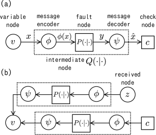
Figure 1: A message flow in erasure BP process: (a) variable to check message flow, (b) check to variable message flow.

II-B Modification of variable node operation

In a conventional erasure BP process, there is no possibility for a variable node to receive contradicting input messages from adjacent check nodes simultaneously. However, in a fault erasure BP process defined above, a variable node may have messages containing both 0 and 1 simultaneously. We thus need to modify the variable node process for accepting such contradicting messages. In this paper, we adopt the following simple modification on the variable node process. If a variable node receives a set of contracting messages that include both 0 and 1, then the variable node sends the erasure symbol to the neighboring check nodes. The same rule is applied to the process for determination of the estimate symbol.

III Density evolution equations

The density evolution (DE) is an important method to unveil the asymptotic behavior of a BP decoding algorithm. In a DE process, we can track the time evolution of the probability distribution of messages (or the probability density function in a case where the messages are continuous). The asymptotic probability distributions obtained by iterative computation tell us the asymptotic quantitative features of the decoding algorithm. In this section, we will derive the DE equations for the fault erasure BP decoder.

III-A Derivation of DE equations

In the following analysis, we will make several assumptions that have been commonly used in related works. The channel is assumed to be a memoryless binary erasure channel (BEC) with the erasure probability $\epsilon(0\leq\epsilon\leq 1)$. In this paper, we consider a regular LDPC code ensemble with the variable node degree $d_{v}$ and the check node degree $d_{c}$. The transmitted word is assumed to be the zero codeword of infinite length.

Suppose that $x$ represents an input to an intermediate node (corresponding to the conditional probability $Q(\cdot|\cdot)$) and that $\hat{x}$ represents the corresponding output from the intermediate node. If $x$ is distributed according to the probability distribution $t(\cdot)$ over the message alphabet $\{0,1,e\}$, then the probability distribution of the output $\hat{x}$ obeys $t^{\prime}(\cdot)$ given by

$$t^{\prime}(\hat{x})=\sum_{x\in\{0,1,e\}}Q(\hat{x}|x)t(x).$$ (17)

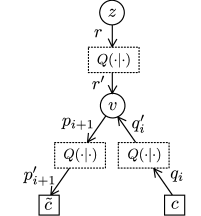
Figure 2: Relation of message probability distributions

In the following, the details of the probability distributions are introduced according to Fig.2. The probability distribution corresponding to the message emitted from a check node $c$ is denote by $q_{i}$. The index $i$ represents the discrete time index in an iterative process. A message from a check node enters an intermediate node, which represents the effect of the probabilistic faults. The distribution corresponds to the output of the intermediate node is represented by $q^{\prime}_{i}$ that is given by

$$q^{\prime}_{i}(\hat{x})=\sum_{x\in\{0,1,e\}}Q(\hat{x}|x)q_{i}(x).$$ (18)

In the following, we will use a convention such that the symbol for the output distribution of the intermediate node is expressed with the symbol of the input distribution with the prime symbol such as $t$ and $t^{\prime}$.

A variable node $v$ computes a message from the set of messages it receives. The message distribution corresponding to the message from a variable node to an intermediate node follows the distribution $p_{i+1}$. The corresponding output distribution from the intermediate node is given by

$$p^{\prime}_{i+1}(\hat{x})=\sum_{x\in\{0,1,e\}}Q(\hat{x}|x)p_{i+1}(x).$$ (19)

We also assume that probabilistic faults may occur in a message flow from a received symbol node to a variable node. A received symbol node send a message in $\{0,1,e\}$ to an intermediate node according to its received value. The probability distribution $r(\cdot)$ of the message is given by

$$r(x)\stackrel{{\scriptstyle\triangle}}{{=}}\left\{\begin{array}[]{ll}1-\epsilon,&x=0,\\ 0,&x=1,\\ \epsilon,&x=e.\\ \end{array}\right.$$ (23)

The message distribution of the corresponding message from the intermediate node follows the distribution

$$r^{\prime}(\hat{x})=\sum_{x\in\{0,1,e\}}Q(\hat{x}|x)r(x).$$ (24)

We first derive the DE equations on the check node output. There are two cases depending on the output of the check node. Firstly, consider the case where the output of the check node is 0. The check node $c$ calculates a message to an adjacent variable node $v$. If and only if the set of $d_{c}-1$ incoming messages received by $c$ except for the one from $v$ contain even number of 1’s and contains no erasure symbols, then the message from $c$ becomes 0. Therefore, the distribution of the check node output $q_{i}(0)$ is given by

$$q_{i}(0) \!=\! \sum_{j:even}^{d_{c}-1}\binom{d_{c}-1}{j}p^{\prime}_{i}(1)^{j}p^{\prime}_{i}(0)^{d_{c}-1-j}$$ (25)

$$\!=\! \frac{(p^{\prime}_{i}(0)\!+\!p^{\prime}_{i}(1))^{d_{c}-1}}{2}\!+\!\frac{{(p^{\prime}_{i}(0)\!-\!p^{\prime}_{i}(1))}^{d_{c}-1}}{2}.$$

The binomial theorem is used in the derivation above. In a similar manner, we can derive $q_{i}(1)$. Note that, in this case, the set of the $d_{c}-1$ messages consisting of odd number of 1’s and no erasure symbols leads to the output message 1 from the check node. We thus have

$$q_{i}(1) \!=\! \sum_{j:odd}^{d_{c}-1}\binom{d_{c}-1}{j}p^{\prime}_{i}(1)^{j}p^{\prime}_{i}(0)^{d_{c}-1-j}$$ (26)

$$\!=\! \frac{(p^{\prime}_{i}(0)\!+\!p^{\prime}_{i}(1))^{d_{c}-1}}{2}\!-\!\frac{{(p^{\prime}_{i}(0)\!-\!p^{\prime}_{i}(1))}^{d_{c}-1}}{2}.$$

We will then consider the DE equations on the variable node output. Let us assume that an output of a variable node is 0, and that the variable node $v$ calculates a message to an adjacent check node $c$. Let $M$ be the set of the $d_{v}-1$ incoming messages to $v$ from adjacent check nodes except for the one from $c$. The variable node message becomes 0 if and only if the event (A) $y=0$ and $1\notin M$ holds, or the event (B) $y=e$, $1\notin M$, and $0\in M$ holds where $y$ received symbols corresponding to the variable node $v$.

The probability corresponding to the event (A) becomes $Prob[A]=r^{\prime}(0)(1-q_{i}^{\prime}(1))^{d_{v}-1}$ because all the incoming messages are independent. The probability of the event (B) is given by $Prob[B]=r^{\prime}(e)\left((1-q^{\prime}_{i}(1))^{d_{v}-1}-q^{\prime}_{i}(e)^{d_{v}-1}\right).$ Since these two events are independent, the probability $p_{i+1}(0)$ is the sum of these two probabilities:

$$p_{i+1}(0) = Prob[A]+Prob[B]$$ (27)

$$= r^{\prime}(0)(1-q^{\prime}_{i}(1))^{d_{v}-1}$$

$$+ r^{\prime}(e)\left((1-q^{\prime}_{i}(1))^{d_{v}-1}-q^{\prime}_{i}(e)^{d_{v}-1}\right).$$

In a similar manner, we can derive the probability corresponding to the variable node message to be $1$:

$$p_{i+1}(1) = r^{\prime}(1)(1-q^{\prime}_{i}(0))^{d_{v}-1}$$ (28)

$$+ r^{\prime}(e)\left((1-q^{\prime}_{i}(0))^{d_{v}-1}-q^{\prime}_{i}(e)^{d_{v}-1}\right).$$

It should be remarked that, for any discrete time index $i$, the equalities $p_{i}(0)+p_{i}(1)+p_{i}(e)=1$ and $q_{i}(0)+q_{i}(1)+q_{i}(e)=1$ hold.

From the arguments above, we have all the DE equations required for the DE analysis of the fault erasure BP decoding. Namely, Based on Eqs. (17)(23)(25)(26)(27)(28) with the initial condition $q_{0}(0)=0,q_{0}(1)=0$, an iterative calculation on the message probability functions leads to the asymptotic message distributions.

III-B Asymptotic error probability

According to the conventional erasure BP rule, if incoming messages to a variable node contain no 1’s and contain a 0, then the tentative estimate of the variable node becomes 0. Let us denote the probability for such an event by $s_{i}(0)$. The probability $s_{i}(0)$ is given by

$$s_{i}(0)=r^{\prime}(0)(1-q^{\prime}_{i}(1))^{d_{v}}+r^{\prime}(e)\left((1-q^{\prime}_{i}(1))^{d_{v}}-q^{\prime}_{i}(e)^{d_{v}}\right).$$ (29)

A DE process can evaluate the asymptotic error probability

$$\gamma(\epsilon,\alpha)\stackrel{{\scriptstyle\triangle}}{{=}}\lim_{i\to\infty}(1-s_{i}(0)).$$ (30)

In the following parts of this paper, we will focus on the behavior of the asymptotic error probability $\gamma(\epsilon,\alpha)$.

IV Numerical results

In the previous section, we derived the DE equations for the fault erasure BP decoder. In this section, numerical results indicating the asymptotic behavior of the decoder will presented.

IV-A Effect of transient faults

Figure 3 presents the asymptotic error probabilities $\gamma(\epsilon,\alpha)$ for $(d_{v},d_{c})=(3,6)$-regular LDPC code ensemble. The four curves depicted in Fig.3 correspond to the fault probabilities $\alpha=10^{-2},10^{-3},10^{-4},10^{-5}$ from left to right. When the fault probability $\alpha$ is equal to 0, the system model exactly coincides with the common erasure BP decoder model without transient faults. In such a case, the asymptotic error probability converges to 0 if $\epsilon$ is greater than the BP threshold $\epsilon_{BP}=0.42944$ (this value is also included in Fig. 3). In the case of positive $\alpha$, the situations are totally different. When $\alpha>0$, we can observe that $\gamma(\epsilon,\alpha)$ converges to positive values due to the faults occurred in the BP decoder. From this figure, it is also seen that smaller $\alpha$ gives smaller $\gamma(\epsilon,\alpha)$. Furthermore, each curve has a sudden (vertical) jump at a certain erasure probability. For example, the curve of $\alpha=10^{-3}$ shows $\gamma(\epsilon,10^{-3})>10^{-1}$ in the regime $\epsilon>0.36207$. On the other hand, in the regime $\epsilon<0.36207$, $\gamma(\epsilon,10^{-3})$ takes the values smaller than $10^{-3}$. The behaviors of the decoder are sharply separated at the erasure probability $\epsilon=0.36207$ that is considered to be a threshold value for the fault erasure BP decoder.

Figure 3: Relationship between erasure probability $\epsilon$ and asymptotic error probability $\gamma(\epsilon,\alpha)$ ((3,6)-regular LDPC code ensemble)

IV-B BP dynamics of fault erasure BP decoder

Figure 4 indicates the dynamics of the BP processes via the evolutions of the pair of the message probabilities $p_{i}(0)$ and $p_{i}(1)$. The ensemble is $(3,6)$-regular LDPC code ensemble and the fault probability is assumed to be $\alpha=10^{-3}$. Each arrow in the figure shows a change of the message probabilities from $(p_{i}(0),p_{i}(1))$ to $(p_{i+1}(0),p_{i+1}(1))$ and each trajectory corresponds to an erasure probability in the range $\epsilon=0.01j(10\leq j\leq 50)$. Since the zero codeword is assumed to be transmitted, the probability $p_{i}(0)$ represents the probability for the correct decoding. It is immediately recognized that there are two groups of the trajectories: one group corresponds to the range $0.37\leq\epsilon\leq 0.5$ and the other group corresponds to the range $0.1\leq\epsilon\leq 0.36$. The trajectories in the first group show the upward movements. This means that the error probability tends to converge to a higher value. On the other hand, the trajectories in the second group indicate that $p_{i}(0)$ approaches to 1 as the number of iterations increases. This numerical results strongly suggest the existence of a bifurcation of this DE evolution processes that can be considered as a non-linear dynamical system. At the erasure probability that corresponds to this bifurcation, we can observe sudden drop of the asymptotic error probability in Fig.3.

Figure 4: Dynamics of BP process: Evolution of message probabilities for variable nodes $p_{i}(0)$ and $p_{i}(1)$ ($(3,6)$-regular LDPC code ensemble，fault probability $\alpha=10^{-3}$)

IV-C Degree and asymptotic error probability

Figure 5 presents the asymptotic error probabilities $\gamma(\epsilon,\alpha)$ for regular-LDPC code ensembles with degrees $(d_{v},d_{c})=(2,4),(3,6),(4,8)$. All the ensembles correspond to the design code rate $1/2$. The fault probability is set to $\alpha=10^{-4}$.

Figure 5: Relationship between erasure probability $\epsilon$ and asymptotic error probability $\gamma(\epsilon,\alpha)$ ($(d_{v},d_{c})$-regular LDPC code ensemble，design code rate 0.5，fault probability $\alpha=10^{-4}$)

From Fig.5, we can observe that the $(d_{v},d_{c})=(3,6)$ ensemble provides the highest fault BP threshold. It is well known that $(3,6)$ ensemble gives the highest threshold in the fault free cases. Similar tendency can be seen in the cases where transient faults exist.

V Message encoding

In the previous section, we observed numerical results of the DE analysis on the fault erasure BP decoder. According to the numerical results, it was shown that we must admit non-zero error probability even in the asymptotic regime if the fault probability is positive. In this section, we discuss and compare two methods for improving the decoding performance of the fault erasure BP decoding at the cost of increased hardware complexity.

The simplest way to improve the decoding performance is to exploit several identical erasure BP decoders in parallel. By using the majority votes from the outputs obtained from these component decoders, we can obtain more reliable estimates of transmitted symbols. In this paper, the scheme is called Majority voting scheme. Another way to enhance the reliability is to use a longer code to protect BP messages. In Section 2, we introduced the message function $\phi$ that encodes a BP message into 2-binary symbols. By replacing the encoding function to an encoding function for a longer code, we can expect that the immunity against possible faults becomes stronger. We call this scheme message encoding. Of course, both schemes (i.e., majority voting and message encoding) require increase of the circuit size that can be considered as the cost should be paid for the improvement of the immunity.

V-A Majority voting scheme

In this subsection, we introduce a simple majority voting scheme that emploies $N$-fault erasure BP decoders for improving the fault immunity. The majority voting scheme determines its output by majority voting based on $N$-outputs from the component BP decoders. Although this scheme requires $N$-fold circuit size compared with the single fault erasure BP decoder, it is expected that the majority voting process improves the asymptotic error probability.

In the following, we will discuss the case where $N=2$. The argument below can be easily extended to general cases where $N>2$. Let $\hat{x}^{(1)},\hat{x}^{(2)}\in\{0,1,e\}$ be the decoder outputs from the two component decoders $D^{(1)}$ and $D^{(2)}$. The majority voting process is defined the function

$$\tau(\hat{x}^{(1)},\hat{x}^{(2)})=\left\{\begin{array}[]{ll}0,&(\hat{x}^{(1)},\hat{x}^{(2)})=(0,0),(0,e),(e,0)\\ e,&(\hat{x}^{(1)},\hat{x}^{(2)})=(0,1),(1,0),(e,e)\\ 1,&(\hat{x}^{(1)},\hat{x}^{(2)})=(1,1),(1,e),(e,1),\\ \end{array}\right.$$

where the function $\tau$ represents the output from the majority voting decoder. We denote the asymptotic error probability for the majority voting scheme by $\gamma_{maj}(\epsilon,\alpha)$.

In the following, a lower bound on $\gamma_{maj}(\epsilon,\alpha)$ will be discussed. Throughout the following argument, we assume that

$$s(0,0) \geq (s(0))^{2}$$ (31)

holds where the quantity $s(0)$ in the righthand side is the asymptotic value of $s_{0}(x)$; i.e., $s(0)=\lim_{i\rightarrow\infty}s_{i}(0),$ which can be evaluated by the density evolution. The quantity $s(0,0)$ is the asymptotic joint probability corresponds to the event that two decoder outputs take the value $(0,0)$. This is a natural assumption because the outputs from the the component decoders $D^{(1)},D^{(2)}$ are expected to be highly correlated. Under the assumption of (31), we can easily derive a lower bound of $\gamma_{maj}(\epsilon,\alpha)$

$$\gamma_{maj}(\epsilon,\alpha)\geq(1-s(0))^{2}.$$ (32)

V-B Details of message encoding

In this subsection, we will introduce a simple message encoding scheme based on a binary code of length $n$. The parameter $n$ is referred to as message code length. In the following, we redefine the encoding and decoding functions. The encoding function $\phi:\{0,1,e\}\rightarrow\{0,1\}^{n}$ is an encoding function now defined by

$$\phi(x)=\left\{\begin{array}[]{ll}\overbrace{00\cdots 0}^{n},&x=0,\\ \overbrace{11\cdots 1}^{n},&x=1,\\ \overbrace{00\cdots 0}^{n/2}\overbrace{11\cdots 1}^{n/2},&x=e.\\ \end{array}\right.$$ (36)

There are several possibilities for choosing decoding functions corresponding to the encoding function defined above. One simple choice is to define a decoding function $\phi$ as

$$\psi(y)=\left\{\begin{array}[]{ll}0,&w_{H}(y)=0\\ 1,&w_{H}(y)=n\\ e,&\mbox{otherwise},\\ \end{array}\right.$$ (40)

where $w_{H}$ represents the Hamming weight function. In this case, the conditional probability $Q(\hat{x}|x)$ corresponding to the intermediate node is given by

$$\left(\begin{array}[]{ccc}(1-\alpha)^{n}&\alpha^{n}&1-(1-\alpha)^{n}-\alpha^{n}\\ \alpha^{n}&(1-\alpha)^{n}&1-(1-\alpha)^{n}-\alpha^{n}\\ \alpha^{\frac{n}{2}}(1-\alpha)^{\frac{n}{2}}&\alpha^{\frac{n}{2}}(1-\alpha)^{\frac{n}{2}}&1-2\alpha^{\frac{n}{2}}(1-\alpha)^{\frac{n}{2}}\\ \end{array}\right).$$

Plugging this condition probability into the DE equations, we can evaluate the asymptotic error probabilities.

V-C Asymptotic error probabilities for message encoding

Figure 6 presents the asymptotic error probabilities of the majority voting decoder (two decoders in parallel, $N=2$) and a fault erasure BP decoder with message encoding $(n=4)$. The $(3,6)$-regular LDPC code ensemble is assumed and the fault probability is set to $\alpha=10^{-4}$. Both schemes can be considered to have comparable circuit sizes. In Fig. 6, the curve of the majority voting decoder corresponds to the lower bound (32). From Fig.6, we can observe that the BP decoder with message encoding archives a higher threshold that those of the single BP decoder and the majority logic decoder. This observation implies that the message encoding has a potential advantage over the majority logic decoder in terms of the decoding performance close to the threshold.

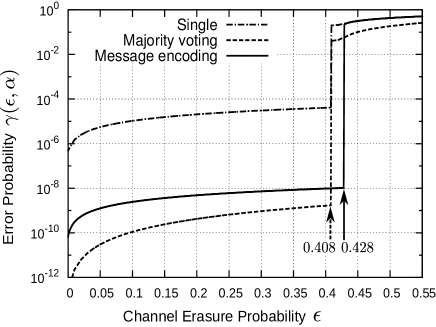
Figure 6: Relationship between erasure probability $\epsilon$ and asymptotic error probability $\gamma(\epsilon,\alpha)$($(3,6)$-regular LDPC code ensemble, fault probability $\alpha=10^{-4}$， message length in message encoding $n=4$，the number of component decoders in majority logic decoder $N=2$)

V-D Choice of message decoding function $\psi$

In a design of an appropriate message encoding scheme, a choice of message decoding function is critical. When $n$ becomes large, we have freedom to choose a message decoding function. In this subsection, we will discuss choices for a message decoding function.

We redefine the message decoding function as

$$\psi(y)\triangleq\left\{\begin{array}[]{ll}0,&0\leq w_{H}(y)\leq k-1,\\ 1,&n-k+1\leq w_{H}(y)\leq n,\\ e,&\mbox{otherwise}.\\ \end{array}\right.$$ (44)

The parameter $k(1\leq k\leq n/2,k\in\mathbb{N})$ controls the decision region for the messages $\{0,1,e\}$. For example, As $k$ gets large, the decision region of $e$ become narrower. Figure 7 presents relationships between the parameter $k$ and the asymptotic error probability $\gamma(\epsilon,\alpha)$. The message code length is assumed to be $n=8$ and the fault probability is set to $\alpha=10^{-4}$.

Figure 7: Relationship between erasure probability $\epsilon$ and asymptotic error probability $\gamma(\epsilon,\alpha)$ ($(3,6)$-regular LDPC code ensemble，fault probability $\alpha=10^{-4}$， code length $n=8$)

From Fig.7, we can see that the asymptotic erasure probabilities depends on the parameter $k$. In this setting, the worst case is $k=4$ and the best case is $k=2$. This result implies that appropriate choice of the message decoding function is important to attain better asymptotic BP decoding performance.

V-E Relationship between code length and asymptotic error probability

Figure 8 presents the asymptotic error probabilities for message code length $n=2,4,8$.

Figure 8: Relationship between erasure probability $\epsilon$ and asymptotic error probability $\gamma(\epsilon,\alpha)$. ($(3,6)$-regular LDPC code ensemble, fault probability $\alpha=10^{-4}$， code length $n=2,4,8$)

Note that we used the optimum parameter for each case such as $k=1(n=2)$, $k=1(n=4)$, and $k=2(n=8)$. The regular LDPC code ensemble with $(d_{v},d_{c})=(3,6)$ is assumed and the fault probability is set to $\alpha=10^{-4}$. From Fig.8, it is observed that the asymptotic error probabilities decreases as code length $n$ increases. However, comparing two cases $n=4$ and $n=8$, we can obtain only small improvement in terms of the fault BP threshold. This means that the major benefit of longer message codes is lowering the error floor of the asymptotic error probability when $n$ is sufficiently large.

VI Conclusion

In this paper, we proposed a model for the fault erasure BP decoders with transient faults. Based on the model, the DE equations were derived and used for numerical evaluation. The DE analysis shows the asymptotic behaviors of the fault erasure BP decoder. The most notable result revealed via the DE analysis is that the asymptotic error probability converges to a positive value in contrast to the the fault free case. The sudden drop of error probability at a certain erasure probability is considered to be a consequence of a bifurcation of the DE dynamical system. In order to improve the decoding performance, we presented two schemes: the message encoding scheme and the majority voting scheme. The result of the DE analysis indicates that the message encoding scheme has clear advantage over the majority voting scheme in terms of the fault erasure BP threshold.

References

- [1] Semiconductor Industry Association, “International Technology Roadmap for Semi-conductors (ITRS),” 2011.
- [2] J. Han and P. Jonker, “A defect-and fault-tolerant architecture for nanocomputers,” Nanotechnology, vol. 14, no. 2, pp. 224-230, Feb. 2003.
- [3] D. K. Pradhan, “Fault-tolerant computer system design,” Upper Saddle River, NJ: Prentice Hall, 1996.
- [4] B. W. Jonson, “Design and analysis of fault-tolerant digital systems,” Reading, MA: Addison-Wesley Publishing Company 1989.
- [5] K. Santanu, C. Santanu, “The next generation of system-on-chip integration,” CRC Press, Oct. 2014.
- [6] H. Wang, “Hardware designs for LT coding,” MSc Thesis, Department of Electrical Engineering, Delft University of Technology, 2004.
- [7] L. R. Varshey, “Performance of LDPC codes under faulty iterative decoding,” IEEE Trans. Inf. Theory, vol. 57, no. 7, pp. 4427-4444, July 2011.
- [8] S. M. S. Tabatabaei, H. Cho, and L. Dolecek, “Gallager B decoder on noisy hardware,” IEEE Trans. Commun. vol. 61, no. 5, pp. 1660-1675, May 2013.
- [9] C. K. Ngassa, V. Savin, and D. Declercq, “Min-sum-based decoders running on noisy hardware,” in Proc. IEEE Global Commun. Conference, 2013.
- [10] A. Balatsoukas-Stimming and A. Burg, “Density evolution for min-sum decoding of LDPC codes under unreliable message storage,” IEEE Commun. Lett, vol. 18, no. 5, pp. 849-852, May 2014.
- [11] C. H. Huang, Y. Li, and L. Dolecek, “Gallager B LDPC decoder with transient and permanent errors,” IEEE Transactions on Communications, vol. 62, no. 1, pp. 15-28, Jan. 2014.
- [12] B. Vasic, P. Ivanis, S. Brkic, and V. Ravanmehr, “Fault-resilient decoders and memories made of unreliable components,” in Proc. Inf. theory and Applications Workshop (ITA 2015), San Diego, CA, paper 273, Feb. 2015.
- [13] J. von Neumann, “Probabilistic logic and the synthesis of reliable organisms from unreliable components,” Automata Studies, vol. 34, pp. 43-98, 1956.