Precision measurement of the $\eta\to\pi^{+}\pi^{-}\pi^{0}$ Dalitz plot distribution
with the KLOE detector

Abstract

Using $1.6$ fb^-1 of $e^{+}e^{-}\to\phi\to\eta\gamma$ data collected with the KLOE detector at DA$\Phi$NE, the Dalitz plot distribution for the $\eta\to\pi^{+}\pi^{-}\pi^{0}$ decay is studied with the world’s largest sample of $\sim 4.7\cdot 10^{6}$ events. The Dalitz plot density is parametrized as a polynomial expansion up to cubic terms in the normalized dimensionless variables $X$ and $Y$. The experiment is sensitive to all charge conjugation conserving terms of the expansion, including a $gX^{2}Y$ term. The statistical uncertainty of all parameters is improved by a factor two with respect to earlier measurements.

I Introduction

The isospin violating $\eta\to\pi^{+}\pi^{-}\pi^{0}$ decay can proceed via electromagnetic interactions or via strong interactions due to the difference between the masses of $u$ and $d$ quarks. The electromagnetic part of the decay amplitude is long known to be strongly suppressed sutherland66 ; sutherland_bell68 . The recent calculations performed at next-to-leading order (NLO) of the chiral perturbation theory (ChPT) baur_kambor_wyler96 ; ditsche_kubis_meissner2009 reaffirm that the decay amplitude is dominated by the isospin violating part of the strong interaction.

Defining the quark mass ratio, $Q$, as

$$Q^{2}\equiv\frac{m_{s}^{2}-\hat{m}^{2}}{m_{d}^{2}-m_{u}^{2}}\qquad\text{ with }\hat{m}=\frac{1}{2}(m_{d}+m_{u}),$$ (1)

the decay width at up to NLO ChPT is proportional to $Q^{-4}$ bijnens_gasser2002 . The definition in Eq. (1), neglecting $\hat{m}^{2}/m_{s}^{2}$, gives an ellipse in the $m_{s}/m_{d},m_{u}/m_{d}$ plane with major semi-axis $Q$ leutwyler96 : a determination of $Q$ puts a stringent constraint on the light quark masses.

Using Dashen’s theorem dashen69 to account for the electromagnetic effects, $Q$ can be determined at the lowest order from a combination of kaon and pion masses. With this value of $Q=24.2$, the ChPT results for the $\eta\to\pi^{+}\pi^{-}\pi^{0}$ decay width at LO, $\Gamma_{LO}=66$ eV, and NLO, $\Gamma_{NLO}=160\pm 50$ eV gasser_leutwyler85_eta3pi , are far from the experimental value $\Gamma_{exp}=300\pm 11$ eV PDG14 . The discrepancy could originate from higher order contributions to the decay amplitude or from the corrections to the $Q$ value.

Several theoretical efforts have aimed at a better description of the $\eta\to 3\pi$ decay amplitude. A full NNLO ChPT calculation has been performed bijnens_ghorbani2007 . However, it depends on the values of a large number of the coupling constants of the chiral lagrangian which are not known precisely and therefore is affected by large uncertainties. A calculation in unitarized ChPT using relativistic coupled channels borasoy_nissler2005 gives better agreement with the data but it is model dependent. With a non-relativistic effective field theory framework, the effects of higher order isospin breaking in the final state interactions have been investigated schneider_kubis_ditsche2011 . The $\pi\pi$ rescattering seems to play an important role in this decay, giving about half of the correction in going from LO to NLO gasser_leutwyler85_eta3pi . The rescattering can be accounted for to all orders using dispersive integrals. In this framework, there are three approaches to improve the ChPT predictions kampf_knecht_novotny_zdrahal2011 ; colangelo_lanz_leutwyler_passemar2011 ; guo2015 . The reliability of the ChPT calculations could be checked by a comparison with the experimental pion distributions represented by the Dalitz plot. Conversely, precise experimental distributions could be used directly for the dispersive analyses kampf_knecht_novotny_zdrahal2011 ; colangelo_lanz_leutwyler_passemar2011 ; guo2015 to determine the $Q$ ratio without relying on the higher order ChPT calculations.

For the $\eta\to\pi^{+}\pi^{-}\pi^{0}$ Dalitz plot distribution, the normalized variables $X$ and $Y$ are commonly used:

$$X =\sqrt{3}\frac{T_{\pi^{+}}-T_{\pi^{-}}}{Q_{\eta}}$$ (2)

$$Y =\frac{3T_{\pi^{0}}}{Q_{\eta}}-1$$ (3)

with

$$Q_{\eta} =T_{\pi^{+}}+T_{\pi^{-}}+T_{\pi^{0}}=m_{\eta}-2m_{\pi^{+}}-m_{\pi^{0}}.$$ (4)

$T_{i}$ are kinetic energies of the pions in the $\eta$ rest frame. The squared amplitude of the decay is parametrized by a polynomial expansion around $(X,Y)=(0,0)$:

$$|A(X,Y)|^{2} \simeq N(1+$$

$$aY+bY^{2}+cX+dX^{2}+eXY+$$

$$fY^{3}+gX^{2}Y+hXY^{2}+lX^{3}+\ldots).$$

The Dalitz plot distribution can then be fit using this formula to extract the parameters $a,b,\ldots$, usually called the Dalitz plot parameters. Note that coefficients multiplying odd powers of $X$ ($c,e,h$ and $l$) must be zero assuming charge conjugation invariance.

The experimental values of the Dalitz plot parameters are shown in Tab. 1 together with the parametrization of theoretical calculations. The most precise previous measurement is from KLOE 2008 analysis which was based on $1.34\cdot 10^{6}$ events kloe2008 . There is some disagreement among the experiments, specially for the $b$ but also for the $a$ parameter. Looking at the theory, both the $b$ and the $f$ parameters deviate from experiment. The new high statistics measurement presented in this paper can help to clarify the tension among the experimental results, and can be used as a more precise input for the dispersive calculations.

Table 1: Summary of Dalitz plot parameters from experiments and theoretical predictions.

Experiment	$-a$	$b$	$d$	$f$	$-g$
Gormley(70) gormley70	$1.17\pm 0.02$	$0.21\pm 0.03$	$0.06\pm 0.04$	$-$	$-$
Layter(73) layter73	$1.080\pm 0.014$	$0.03\pm 0.03$	$0.05\pm 0.03$	$-$	$-$
CBarrel(98) CBarrel98	$1.22\pm 0.07$	$0.22\pm 0.11$	$0.06$(fixed)	$-$	$-$
KLOE(08) kloe2008	$1.090\pm 0.005^{+0.019}_{-0.008}$	$0.124\pm 0.006\pm 0.010$	$0.057\pm 0.006^{+0.007}_{-0.016}$	$0.14\pm 0.01\pm 0.02$	$-$
WASA(14) patrik2014	$1.144\pm 0.018$	$0.219\pm 0.019\pm 0.047$	$0.086\pm 0.018\pm 0.015$	$0.115\pm 0.037$	$-$
BESIII(15) besIII2015	$1.128\pm 0.015\pm 0.008$	$0.153\pm 0.017\pm 0.004$	$0.085\pm 0.016\pm 0.009$	$0.173\pm 0.028\pm 0.021$	$-$
Calculations
ChPT LO bijnens_ghorbani2007	1.039	0.27	0	0	$-$
ChPT NLO bijnens_ghorbani2007	1.371	0.452	0.053	0.027	$-$
ChPT NNLO bijnens_ghorbani2007	$1.271\pm 0.075$	$0.394\pm 0.102$	$0.055\pm 0.057$	$0.025\pm 0.160$	$-$
dispersive kambor_wiesendanger_wyler96	1.16	0.26	0.10	$-$	$-$
simplified disp bijnens_gasser2002	1.21	0.33	0.04	$-$	$-$
NREFT schneider_kubis_ditsche2011	$1.213\pm 0.014$	$0.308\pm 0.023$	$0.050\pm 0.003$	$0.083\pm 0.019$	$0.039\pm 0.002$
UChPT borasoy_nissler2005	$1.054\pm 0.025$	$0.185\pm 0.015$	$0.079\pm 0.026$	$0.064\pm 0.012$	$-$

II The KLOE detector

The KLOE detector at the DA$\Phi$NE $e^{+}e^{-}$ collider in Frascati consists of a large cylindrical Drift chamber (DC) and an electromagnetic calorimeter (EMC) in a 0.52 T axial magnetic field. The DC KLOEDCNIM is 4 m in diameter and 3.3 m long and is operated with a helium - isobutane gas mixture (90% - 10%). Charged particles are reconstructed with a momentum resolution of $\sigma(p_{\perp})/p_{\perp}\simeq 0.4\%$.

The EMC KLOEEMCNIM consists of alternating layers of lead and scintillating fibers covering 98% of the solid angle. The lead-fiber layers are arranged in $\sim(4.4\times 4.4)\text{ cm}^{2}$ cells, five in depth, and these are read out at both ends. Hits in cells close in time and space are grouped together in clusters. Cluster energy is obtained from the signal amplitude and has a resolution of $\sigma(E)/E=5.7\%/\sqrt{E(\text{GeV)}}$. Cluster time, $t_{\rm cluster}$, and position are energy weighted averages, with time resolution $\sigma(t)=(57\text{ ps})/\sqrt{E(\text{GeV)}}\oplus 100$ ps. The cluster position along the fibers is obtained from time differences of the signals.

The KLOE trigger KLOEtrigger uses both EMC and DC information. The trigger conditions are chosen to minimize beam background. In this analysis, events are selected with the calorimeter trigger, requiring two energy deposits with $E>50$ MeV for the barrel and $E>150$ MeV for the endcaps.

The analysis is performed using data collected at the $\phi$ meson peak with the KLOE detector in 2004-2005, and corresponds to an integrated luminosity of $\sim 1.6\text{ fb}^{-1}$. Due to DA$\Phi$NE crossing angle $\phi$ mesons have a small horizontal momentum, p_ϕ of about 13 MeV/c. The $\eta$ mesons are produced in the radiative decay $\phi\to\eta\gamma_{\phi}$. The photon from the $\phi$ radiative decay, $\gamma_{\phi}$, has an energy $E\sim 363$ MeV. The data sample used for this analysis is independent and about four times larger than the one used in the previous KLOE(08) $\eta\to\pi^{+}\pi^{-}\pi^{0}$ Dalitz plot analysis kloe2008 .

The reconstructed data are sorted by an event classification procedure which rejects beam and cosmic ray backgrounds and splits the events into separate streams according to their topology KLOEdatahandling . The beam and background conditions are monitored. The corresponding parameters are stored for each run and included in the GEANT3 based Monte Carlo (MC) simulation of the detector. The event generators for the production and decays of the $\phi$-meson include simulation of initial state radiation. The final state radiation is included for the simulation of the signal process. The simulation of $e^{+}e^{-}\to\omega\pi^{0}$ process (an important background in this analysis) assumes a cross section of $8$ nb. The simulations of the background channels used in this analysis correspond to the integrated luminosity of the experimental data set, while the signal simulation corresponds to ten times larger luminosity.

III Event Selection

Two tracks of opposite curvature and three neutral clusters are expected in the final state of the chain $e^{+}e^{-}\to\phi\to\eta\gamma_{\phi}\to\pi^{+}\pi^{-}\pi^{0}\gamma_{\phi}\to\pi^{+}\pi^{-}\gamma\gamma\gamma_{\phi}$. Selection steps are listed below:

• A candidate event has at least three prompt neutral clusters in the EMC. The clusters are required to have energy at least 10 MeV and polar angles $23^{\circ}<\theta<157^{\circ}$, where $\theta$ is calculated from the distance of the cluster to the beam crossing point ($R_{\text{cluster}}$). The time of the prompt clusters should be within the time window for massless particles, $|t_{\text{cluster}}-R_{\text{cluster}}/c|<5\sigma(t)$, while neutral clusters do not have an associated track in the DC.

• At least one of the prompt neutral clusters has energy greater than 250 MeV. The highest energy cluster is assumed to originate from the $\gamma_{\phi}$ photon.

• The two tracks with smallest distance from the beam crossing, and with opposite curvature, are chosen. In the following these tracks are assumed to be due to charged pions. Discrimination against electron contamination from Bhabha scattering is achieved by means of Time Of Flight as discussed in the following.

• $P_{\phi}$, the four-momentum of the $\phi$ meson, is determined using the beam-beam energy $\sqrt{s}$ and the $\phi$ transverse momentum measured in Bhabha scattering events for each run.

• The $\gamma_{\phi}$ direction is obtained from the position of the EMC cluster while its energy/momentum is calculated from the two body kinematics of the $\phi\to\eta\gamma_{\phi}$ decay:

  $$E_{\gamma_{\phi}}=\frac{m_{\phi}^{2}-m_{\eta}^{2}}{2\cdot\left(E_{\phi}-|{\bf p}_{\phi}|\cos\theta_{\phi,\gamma}\right)}$$

  where $\theta_{\phi,\gamma}$ is the angle between the $\phi$ and the $\gamma_{\phi}$ momenta. The four-momentum of the $\eta$ meson is then: $P_{\eta}=P_{\phi}-P_{\gamma_{\phi}}$.

• The $\pi^{0}$ four-momentum is calculated from the missing four-momentum to $\eta$ and the charged pions: $P_{\pi^{0}}=P_{\eta}-P_{\pi^{+}}-P_{\pi^{-}}$.

• To reduce the Bhabha scattering background, the following two cuts are applied:

  • a cut in the ($\theta_{+\gamma}$,$\theta_{-\gamma}$) plane as shown in Fig. 1, where $\theta_{+\gamma}(\theta_{-\gamma})$ is the angle between the $\pi^{+}(\pi^{-})$ and the closest photon from $\pi^{0}$ decay.

  • a cut in the $(\Delta t_{e},\Delta t_{\pi})$ plane as shown in Fig. 2, to discriminate electrons from pions, where $\Delta t_{e}$, $\Delta t_{\pi}$ are calculated for tracks which have an associated cluster, $\Delta t_{e/\pi}\equiv t_{\text{track}_{e/\pi}}-t_{\text{cluster}}$, where $t_{\text{track}_{e/\pi}}$, is the expected arrival time to EMC for $e/\pi$ with the measured momentum, and $t_{\text{cluster}}$ the measured time of the EMC cluster.

• To improve the agreement between simulation and data, a correction for the relative yields of: (i) $e^{+}e^{-}\to\omega\pi^{0}$, and (ii) sum of all other backgrounds, with respect to the signal is applied. The correction factors are obtained from a fit to the distribution of the azimuthal angle between the $\pi^{0}$ decay photons, in the $\pi^{0}$ rest frame, $\theta_{\gamma\gamma}^{*}$ (Fig. 3). The uncertainties of the correction factors are evaluated by comparing the corresponding fit to the distribution of the missing mass squared, $P_{\pi^{0}}^{2}$ (Fig. 4).

• To further reduce the background contamination, two more cuts are applied:

  • $\theta_{\gamma\gamma}^{*}>165^{\circ}$, see Fig. 3;

  • $\left||P_{\pi^{0}}|-m_{\pi^{0}}\right|<15$ MeV, see Fig. 4;

The overall signal efficiency is 37.6% at the end of the analysis chain and the signal to background ratio is 133.

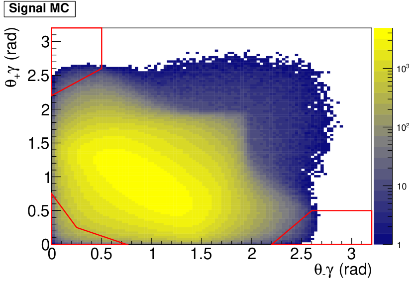
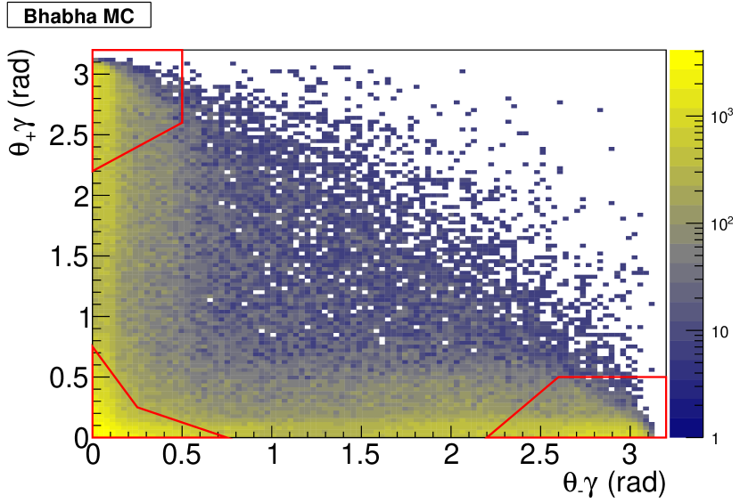
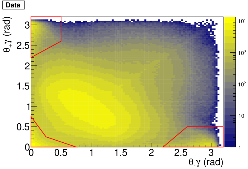
Figure 1: (Color online) $\theta_{+\gamma}$ vs $\theta_{+\gamma}$ angle plot. The three panels correspond to signal MC, Bhabha MC and the data. The three regions in the corners with borders marked by red lines represent the Bhabha rejection cut applied in the analysis.

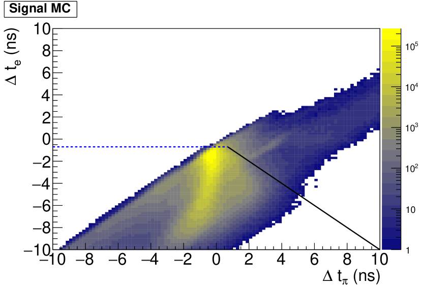
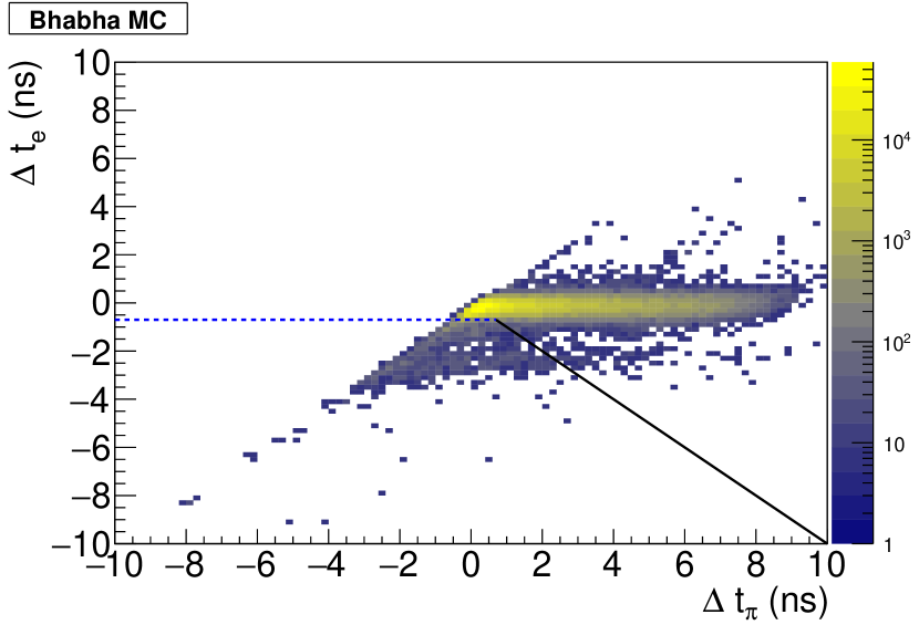
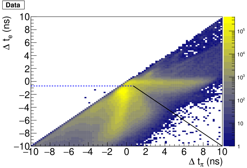
Figure 2: (Color online) $\Delta t_{e}$ vs $\Delta t_{\pi}$ plots for signal MC, Bhabha MC and the data. Events above the blue (dotted) line or above the black (full) line are rejected.

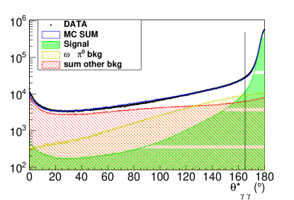
Figure 3: (Color online) Azimuthal angle difference between the $\pi^{0}$ decay photons in the $\pi^{0}$ rest frame, $\theta^{*}_{\gamma\gamma}$, with the MC contributions scaled. The cut $\theta^{*}_{\gamma\gamma}>165^{\circ}$ is shown by the vertical line.

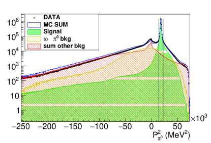
Figure 4: (Color online) Missing mass squared, $P_{\pi^{0}}^{2}$, with the MC contributions scaled. The cut $\left||P_{\pi^{0}}|-m_{\pi^{0}}\right|<15$ MeV is represented by the two vertical lines.

As can be seen in Figs. 3, 4 and 5 the agreement of simulation with the experimental data is good.

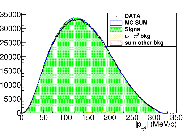
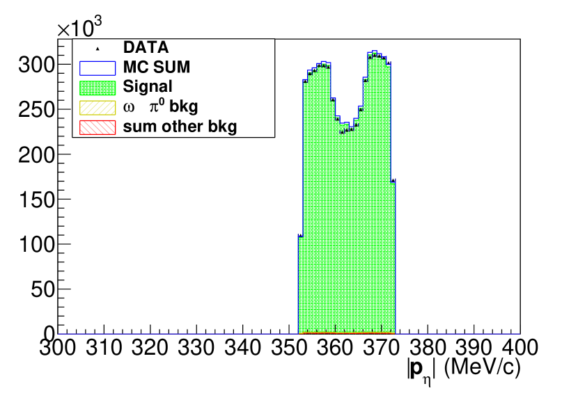
Figure 5: Distribution of the reconstructed momentum of $\pi^{0}$ (left) and $\eta$ (right) for the data and MC.

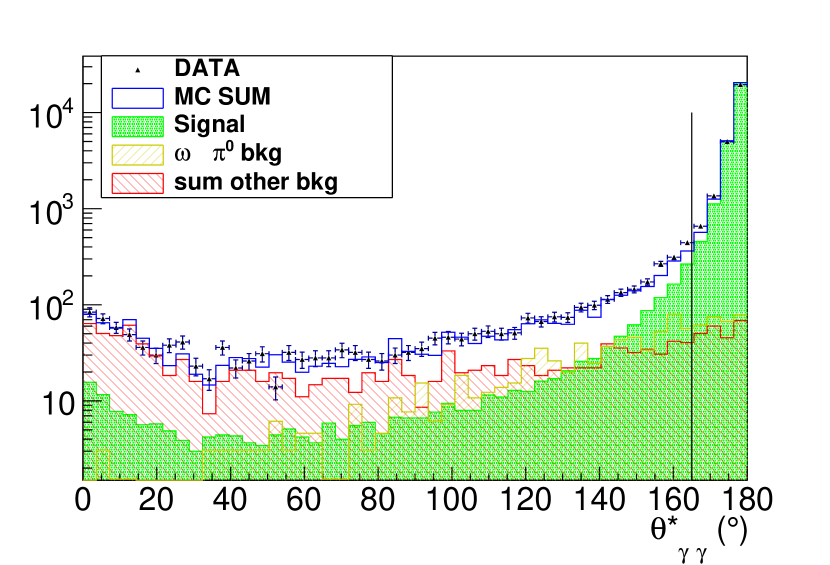
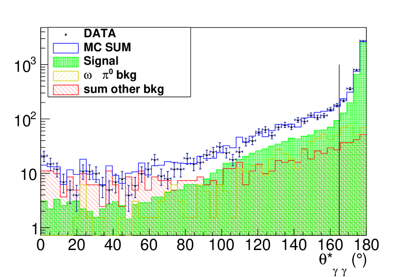
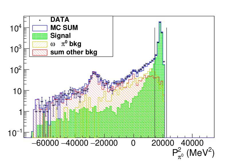
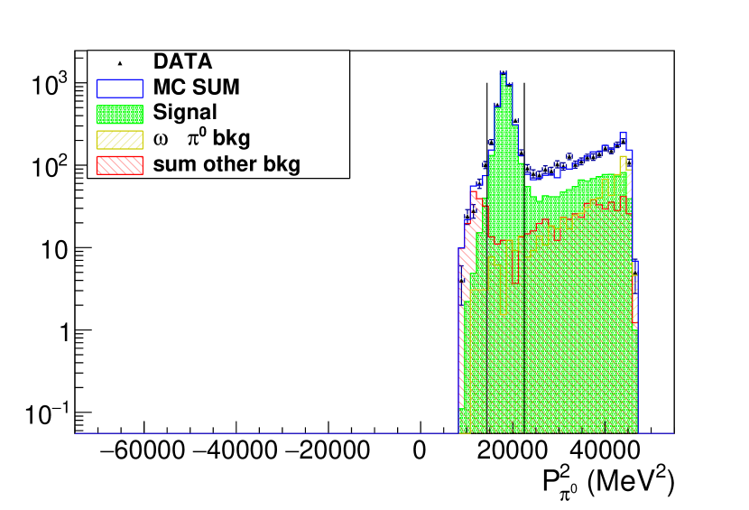
Figure 6: (Color online) Top: $\theta_{\gamma\gamma}^{*}$ angle distribution with the MC contributions scaled; the selected region is at the right of the vertical line. Bottom: missing mass squared,$P_{\pi^{0}}^{2}$, with the MC contributions scaled. The selected region is between the vertical lines. Left/right: bin of the Dalitz plot with the largest/smallest number of entries, corresponding to $(X,Y)=(0.000,-0.850)$ and $(X,Y)=(-0.065,0.750)$, respectively.

IV Dalitz Plot

For the Dalitz plot, a two dimensional histogram representation is used. The bin width is determined both by the resolution in the $X$ and $Y$ variables and the number of events in each bin, which should be large enough to justify $\chi^{2}$ fitting. The resolution of the $X$ and $Y$ variables is evaluated with MC signal simulation. The distribution of the difference between the true and reconstructed values is fit with a double Gaussian. The standard deviations of the narrower Gaussians are $\delta_{X}=0.021$ and $\delta_{Y}=0.032$. The range $(-1,1)$ for the $X$ and $Y$ variables was divided into 31 and 20 bins, respectively. Therefore the bin widths correspond to approximately three standard deviations. The minimum bin content is $3.3\cdot 10^{3}$ events. Fig. 6 shows the distributions of the $\theta_{\gamma\gamma}^{*}$ and the $P_{\pi^{0}}^{2}$ variables for two bins in the Dalitz plot, one with the largest content and one with the smallest. As can be seen, the signal and the background are well reproduced by the simulation.

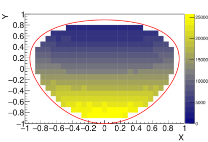
Figure 7: (Color online) The experimental background subtracted Dalitz plot distribution represented by the two dimensional histogram with 371 bins. Only bins used for the Dalitz parameter fits are shown. The physical border is indicated by the red line.

Fig. 7 shows the experimental Dalitz plot distribution after background subtraction, which is fit to the amplitude expansion from Eq. (I) to extract the Dalitz plot parameters. Only $n=371$ bins which are fully inside the kinematic boundaries are used and there are $\sim 4.7\cdot 10^{6}$ entries in the background subtracted Dalitz plot.

The fit is performed by minimizing the $\chi^{2}$ like function

$$\chi^{2}=\sum_{i=1}^{n}\left(\frac{N_{i}-\sum_{j=1}^{n_{T}}S_{ij}N_{T,j}}{\sigma_{i}}\right)^{2}$$ (6)

where:

• $N_{T,j}=\int|A(X,Y)|^{2}dPh(X,Y)_{j}$, with $|A(X,Y)|^{2}$ given by Eq. (I). The integral is over $X$ and $Y$ in the allowed phase space for bin $j$. The sum over $j$ bins includes all Dalitz plot bins at least partly inside the physical border, $n_{T}$.

• $N_{i}=N_{data,i}-\beta_{1}B_{i1}-\beta_{2}B_{i2}$ is the background subtracted content of Dalitz plot bin $i$, where $\beta_{1,2}$ are the scaling factors, $B_{i1}$ is the $\omega\pi^{0}$ background in the bin $i$ and $B_{i2}$ is the same for the remaining background.

• $S_{ij}$ is the acceptance and smearing matrix from bin $j$ to bin $i$ in the Dalitz plot. It is determined from signal MC by $S_{ij}={N_{rec,i;gen,j}}/{N_{gen,j}}$, where $N_{rec,i;gen,j}$ denotes the number of events reconstructed in bin $i$ which were generated in bin $j$ and $N_{gen,j}$ denotes the total number of events generated in bin $j$.

• $\sigma_{i}^{2}=\sigma_{N_{i}}^{2}+\sigma_{S_{ij}}^{2}$ is the error in bin $i$, with $\sigma_{S_{ij}}^{2}=\sum_{j=1}^{n_{T}}N_{T,j}^{2}\cdot{S_{ij}\cdot(1-S_{ij})}/{N_{gen,j}}$.

The input-output test of the fit procedure was performed using signal MC generated with the same statistics as the experimental data. The extracted values for the parameters were within one standard deviation with respect to the input.

Table 2: Results for the Dalitz plot parameter fits. Fit $\#4$ includes the $g$ parameter, while fit $\#3$, with $g=0$, can be directly compared to previous results. The fits $\#5$ and $\#6$ use the acceptance corrected data (see Appendix A).

Fit/set#	$a$	$b\cdot 10$	$d\cdot 10^{2}$	$f\cdot 10$	$g\cdot 10^{2}$	$c,e,h,l$	$\chi^{2}/$dof	Prob
(1)	$-1.095\pm 0.003$	$1.454\pm 0.030$	$8.11\pm 0.32$	$1.41\pm 0.07$	$-4.4\pm 0.9$	free	$354/361$	0.60
(2)	$-1.104\pm 0.002$	$1.533\pm 0.028$	$6.75\pm 0.27$	$0$	$0$	$0$	$1007/367$	$0$
(3)	$-1.104\pm 0.003$	$1.420\pm 0.029$	$7.26\pm 0.27$	$1.54\pm 0.06$	$0$	$0$	$385/366$	0.24
(4)	$-1.095\pm 0.003$	$1.454\pm 0.030$	$8.11\pm 0.33$	$1.41\pm 0.07$	$-4.4\pm 0.9$	$0$	$360/365$	0.56
(5)	$-1.092\pm 0.003$	$1.45\pm 0.03$	$8.1\pm 0.3$	$1.37\pm 0.06$	$-4.4\pm 0.9$	$0$	$369/365$	0.43
(6)	$-1.101\pm 0.003$	$1.41\pm 0.03$	$7.2\pm 0.3$	$1.50\pm 0.06$	$0$	$0$	$397/366$	0.13

The fit has been performed using different choices of the free parameters in Eq. (I), with the normalization $N$ and the parameters $a$, $b$ and $d$ always let free. The main fit results are summarized in Tab. 2. The first row (set #1) includes all parameters of the cubic expansion, Eq. (I). The fit values of the charge conjugation violating parameters $c,e,h$ and $l$ are consistent with zero ($c=(4.3\pm 3.4)\cdot 10^{-3}$, $e=(2.5\pm 3.2)\cdot 10^{-3}$, $h=(1.1\pm 0.9)\cdot 10^{-2}$, $l=(1.1\pm 6.5)\cdot 10^{-3}$) and are omitted from the table. Therefore in all remaining fits the charge conjugation violating parameters $c,e,h$ and $l$ are set to zero. The result #2 with $f=g=0$ demonstrates that it is not possible to describe the distribution with only quadratic terms. The fits including in addition the $f$ parameter improves the accuracy largely providing a good description. A complementary test with $f$ fixed to zero and free $g$ parameter leads to much worse $\chi^{2}$ value. This observation is consistent with the recent experimental results that used the same free parameters, in particular the KLOE(08) analysis. In the set #4 which includes both $f$ and $g$ parameters in the fit, the $g$ parameter differs from zero at the $4.9\sigma$ level and the fit probability is as good as for the fit #1. For completeness in the further discussions we include also set #3 with $g=0$, since it enables direct comparison to the previous experiments (KLOE(08), WASA(14) and BESIII(15)). The correlation matrices for fits #3 and #4 are:

	$b$	$d$	$f$
$a$	$-0.269$	$-0.365$	$-0.832$
$b$		$+0.333$	$-0.139$
$d$			$+0.089$

	$b$	$d$	$f$	$g$
$a$	$-0.120$	$+0.044$	$-0.859$	$-0.534$
$b$		$+0.389$	$-0.201$	$-0.225$
$d$			$-0.160$	$-0.557$
$f$				$+0.408$.

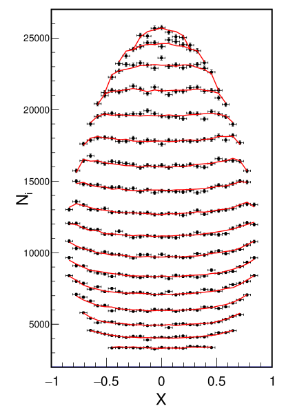
Figure 8: (Color online) The experimental background subtracted Dalitz plot data, $N_{i}$, (points with errors), compared to set #4 fit results (red lines connecting bins with the same $Y$ value). The row with lowest $N_{i}$ values corresponds to the highest $Y$ value ($Y=+0.75$).

The fit #4 is compared to the background subtracted Dalitz plot data, $N_{i}$, in Fig. 8. The red lines represent the fit result and correspond to separate slices in the $Y$ variable. Fig. 9 shows the distribution of the normalized residuals for the fit #4: $r_{i}=(N_{i}-\sum_{j=1}^{n}S_{ij}N_{T,j})/\sigma_{i}$. The location of the residuals $r_{i}>1$ and $r_{i}<-1$ on the Dalitz plot is uniform. The fits $\#5$ and $\#6$ use the acceptance corrected data (see Appendix A).

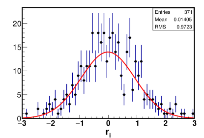
Figure 9: (Color online) Distribution of the normalized residuals, $r_{i}$, for fit #4.

V Asymmetries

While the extracted Dalitz plot parameters are consistent with charge conjugation symmetry, the unbinned integrated charge asymmetries provide a more sensitive test. The left-right ($A_{LR}$), quadrant ($A_{Q}$) and sextant ($A_{S}$) asymmetries are defined in Ref. layter72_asym . The same background subtraction is applied as for the Dalitz plot parameter analysis. For each region in the Dalitz plot used in the calculation of the asymmetries, the acceptance is calculated from the signal MC as the ratio between the number of the reconstructed and the generated events. The yields are then corrected for the corresponding efficiency. The procedure was tested using signal MC generated with the same statistics as the experimental data.

VI Systematic Checks

To quantify and account for systematic effects in the results, several checks have been made.

• Minimum photon energy cut (EGmin) is changed from 10 MeV to 20 MeV (for comparison the EMC energy resolution varies from 60% to 40% for this energy range). The systematic error is taken as half of the difference.

• Background subtraction (BkgSub) is checked by determining the background scaling factors for each bin (or region for the asymmetries) of the Dalitz plot separately. With the same method as for the whole data sample, using the $\theta_{\gamma\gamma}^{*}$ and $P_{\pi^{0}}^{2}$ distributions, background scaling factors are determined for each bin (or region). The systematic error is taken as half the difference with the standard result.

• Choice of binning (BIN) is tested by varying number of bins of the Dalitz plot. For $X$ and $Y$ simultaneously, the bin width is varied from $\sim 2\delta_{X,Y}$ to $\sim 5\delta_{X,Y}$, in total 10 configurations. The systematic uncertainty is given by the standard deviation of the results.

• $\theta_{+\gamma},\theta_{-\gamma}$ cut: the areas of the three zones shown in Fig. 1 were simultaneously varied by $\pm 10\%$.

• $\Delta t_{e},\Delta t_{\pi}$ cut: the offsets of the horizontal and diagonal lines shown in Fig. 2 were varied by $\pm 0.22$ ns and $\pm 0.21$ ns, respectively.

• $\theta_{\gamma\gamma}^{*}$ cut is varied by $\pm 3^{\circ}$, corresponding to $\sim 1\sigma$.

• Missing mass cut (MM) is tested by varying the cut by $\pm 2.0$ MeV, $\sim 1\sigma$. For this cut a stronger dependence of the parameters on the cut was noted. This has been further investigated by performing the Dalitz plot parameter fit for one parameter at a time, for each step, and keeping the other parameters fixed at the value for the standard result. Since the dependence was reduced when varying just one parameter, we conclude that it is mostly due to the correlations between parameters.

• Event classification procedure (ECL) is investigated by using a prescaled data sample without the event classification bias (collected with prescaling factor $1/20$). The fraction of events remaining in each Dalitz plot bin after the event classification conditions varies between 94% and 80% for different bins and it is very well described by the MC within the errors. The analysis of the prescaled data follows the standard chain. The systematic error is extracted as half the difference between the results of the analysis with and without the event classification procedure.

Unless stated otherwise the systematic error is calculated as the difference between the two tests and the standard result. If both differences have the same sign, the asymmetric error is taken with one boundary set at zero and the other at the largest of the differences. The resulting systematic error contributions for the Dalitz plot parameters for the sets #4 and #3 are summarized in Tab. 3 and Tab. 4, respectively. The results for the charge asymmetries are summarized in Tab. 5.

Table 3: Summary of the systematic errors for $a,b,d,f,g$ parameters (fit $\#4$ ).

syst. error ($\times 10^{4}$)	$\Delta a$	$\Delta b$	$\Delta d$	$\Delta f$	$\Delta g$
EGmin	$\pm 6$	$\pm 12$	$\pm 10$	$\pm 5$	$\pm 16$
BkgSub	$\pm 8$	$\pm 7$	$\pm 11$	$\pm 6$	$\pm 38$
BIN	$\pm 17$	$\pm 13$	$\pm 9$	$\pm 36$	$\pm 44$
$\theta_{+\gamma},\theta_{-\gamma}$ cut	${}^{+0}_{-1}$	${}^{+0}_{-2}$	${}^{+2}_{-2}$	${}^{+3}_{-0}$	${}^{+3}_{-2}$
$\Delta t_{e}$ cut	${}_{-11}^{+\ 6}$	${}_{-\ 1}^{+12}$	${}_{-\ 1}^{+18}$	${}_{-8}^{+3}$	${}_{-54}^{+26}$
$\Delta t_{e}-\Delta t_{\pi}$ cut	$\pm 0$	${}_{-1}^{+0}$	${}_{-1}^{+3}$	$\pm 0$	${}_{-1}^{+2}$
$\theta_{\gamma\gamma}^{*}$ cut	${}^{+14}_{-\ 5}$	${}^{+2}_{-1}$	${}^{+21}_{-12}$	${}^{+\ 5}_{-25}$	${}^{+26}_{-38}$
MM	${}^{+\ 8}_{-10}$	${}^{+46}_{-43}$	${}^{+49}_{-45}$	${}^{+57}_{-62}$	${}^{+100}_{-\ 92}$
ECL	$\pm 0$	$\pm 8$	$\pm 6$	$\pm 9$	$\pm 12$
TOTAL	${}^{+26}_{-25}$	${}^{+52}_{-48}$	${}^{+59}_{-50}$	${}^{+69}_{-77}$	${}^{+123}_{-129}$

Table 4: Summary of the systematic errors for $a,b,d,f$ parameters (fit $\#3$).

syst. error ($\times 10^{4}$)	$\Delta a$	$\Delta b$	$\Delta d$	$\Delta f$
EGmin	$\pm 9$	$\pm 10$	$\pm 6$	$\pm 0$
BkgSub	$\pm 1$	$\pm 5$	$\pm 6$	$\pm 8$
BIN	$\pm 9$	$\pm 14$	$\pm 9$	$\pm 26$
$\theta_{+\gamma},\theta_{-\gamma}$ cut	${}_{-1}^{+0}$	${}_{-2}^{+0}$	${}_{-1}^{+1}$	${}_{-0}^{+4}$
$\Delta t_{e}$ cut	${}_{-6}^{+0}$	${}_{-\ 6}^{+14}$	${}_{-0}^{+7}$	${}_{-15}^{+19}$
$\Delta t_{e}-\Delta t_{\pi}$ cut	$\pm 0$	${}_{-1}^{+0}$	${}_{-0}^{+3}$	$\pm 0$
$\theta_{\gamma\gamma}^{*}$ cut	${}^{+6}_{-0}$	${}^{+1}_{-1}$	${}^{+14}_{-\ 8}$	${}^{+\ 0}_{-13}$
MM	${}^{+10}_{-10}$	${}^{+39}_{-36}$	${}^{+31}_{-26}$	${}^{+28}_{-35}$
ECL	$\pm 2$	$\pm 9$	$\pm 9$	$\pm 13$
TOTAL	${}^{+18}_{-18}$	${}^{+46}_{-41}$	${}^{+38}_{-31}$	${}^{+45}_{-51}$

Table 5: Summary of the systematic errors for the asymmetries.

syst. error ($\times 10^{5}$)	$\Delta A_{LR}$	$\Delta A_{Q}$	$\Delta A_{S}$
EGmin	$\pm 1$	$\pm 0$	$\pm 4$
BkgSub	$\pm 5$	$\pm 3$	$\pm 16$
$\theta_{+\gamma},\theta_{-\gamma}$ cut	${}^{+2}_{-0}$	${}^{+0}_{-2}$	${}^{+2}_{-0}$
$\Delta t_{e}$ cut	${}_{-92}^{+49}$	${}_{-22}^{+48}$	${}_{-15}^{+\ 7}$
$\Delta t_{e}-\Delta t_{\pi}$ cut	${}^{+0}_{-2}$	${}_{-0}^{+3}$	${}_{-1}^{+0}$
$\theta_{\gamma\gamma}^{*}$ cut	${}^{+\ 1}_{-57}$	${}^{+3}_{-4}$	${}^{+0}_{-8}$
MM	${}^{+0}_{-4}$	${}^{+0}_{-1}$	${}^{+1}_{-2}$
ECL	$\pm 9$	$\pm 0$	$\pm 25$
TOTAL	${}^{+\ 50}_{-109}$	${}^{+48}_{-23}$	${}^{+31}_{-35}$

VII Discussion

The final results for the Dalitz plot parameters, including systematic effects, are therefore:

$$a=- 1.095\pm 0.003^{+0.003}_{-0.002}$$

$$b=+ 0.145\pm 0.003\pm 0.005$$

$$d=+ 0.081\pm 0.003^{+0.006}_{-0.005}$$

$$f=+ 0.141\pm 0.007^{+0.007}_{-0.008}$$

$$g=- 0.044\pm 0.009^{+0.012}_{-0.013}$$

including the $g$ parameter. With $g$ parameter set to zero the results are:

$$a =-1.104\pm 0.003\pm 0.002$$

$$b =+0.142\pm 0.003^{+0.005}_{-0.004}$$

$$d =+0.073\pm 0.003^{+0.004}_{-0.003}$$

$$f =+0.154\pm 0.006^{+0.004}_{-0.005}.$$

These results confirm the tension with the theoretical calculations on the $b$ parameter, and also the need for the $f$ parameter. In comparison to the previous measurements shown in Tab. 1, the present results are the most precise and the first including the $g$ parameter. The improvement over KLOE(08) analysis comes from four times larger statistics and improvement in the systematic uncertainties which are in some cases reduced by factor $2-3$. The major improvement in the systematic uncertainties comes from the analysis of the effect of the Event classification with an unbiased prescaled data sample.

The final values of the charge asymmetries are all consistent with zero:

$$A_{LR} =(-5.0\pm 4.5^{+5.0}_{-11})\cdot 10^{-4}$$

$$A_{Q} =(+1.8\pm 4.5^{+4.8}_{-2.3})\cdot 10^{-4}$$

$$A_{S} =(-0.4\pm 4.5^{+3.1}_{-3.5})\cdot 10^{-4}.$$

The systematic and statistical uncertainties are of the same size except for the $A_{LR}$ which is dominated by the systematic uncertainty due to the description of the Bhabha background.

Appendix A Acceptance corrected data

With a smearing matrix close to diagonal and the smearing to and from nearby bins symmetrical, the acceptance corrected data can be used instead of dealing with the smearing matrix. This representation has the advantage of being much easier to compare directly with theoretical calculations. The acceptance corrected signal content in each bin of the Dalitz plot is obtained by dividing the background subtracted content, $N_{i}$, by the corresponding acceptance, $\epsilon_{i}$. The acceptance is obtained from the signal MC by dividing the number of reconstructed events allocated to the bin $i$ by the number of generated (unsmeared) signal events in that bin.

The fit to extract the Dalitz plot parameters values is done now by minimizing

$$\chi^{2}=\sum_{i=1}^{n}\left(\frac{N_{i}/\epsilon_{i}-N_{T,i}}{\sigma_{i}}\right)^{2}$$ (7)

where the sum includes only bins completely inside the Dalitz plot boundaries and $N_{T,i}=\int\int|A(X,Y)|^{2}dX_{i}dY_{i}$. The statistical uncertainty $\sigma_{i}$ includes contributions from the experimental data, the background estimated from MC and the efficiency. The fitted Dalitz plot parameters using the acceptance corrected data are presented in Tab. 2 as sets $\#5$ with $g$ parameter and $\#6$ with $g=0$. The results are identical within statistical uncertainties with the values obtained using the smearing matrix. Therefore the acceptance corrected data can be used to represent the measured Dalitz plot density if one neglects systematical uncertainties. The table containing Dalitz plot acceptance corrected data (normalized to the content of the $X_{c}=0.0,Y_{c}=0.05$ bin), is provided as a supplementary material (file DPhist_acccorr.txt). The correlation matrix for the fit #5 reads:

	$b$	$d$	$f$	$g$
$a$	$-0.110$	$+0.006$	$-0.849$	$-0.512$
$b$		$+0.397$	$-0.216$	$-0.239$
$d$			$-0.133$	$-0.537$
$f$				$+0.380$.

References

- (1) D. Sutherland, Phys. Lett. 23, 384 (1966).
- (2) J. Bell and D. Sutherland, Nucl.Phys. B4, 315 (1968).
- (3) R. Baur, J. Kambor and D. Wyler, Nucl.Phys. B460, 127 (1996).
- (4) C. Ditsche, B. Kubis and U.-G. Meißner, Eur.Phys.J. C60, 83 (2009).
- (5) J. Bijnens and J. Gasser, Phys.Scripta T99, 34 (2002).
- (6) H. Leutwyler, Phys.Lett. B378, 313 (1996).
- (7) R. Dashen, Phys. Rev. 183, 1245 (1969).
- (8) J. Gasser and H. Leutwyler, Nucl.Phys. B250, 539 (1985).
- (9) K. A. Olive et al. (Particle Data Group), Chin.Phys. C38, 090001 (2014).
- (10) J. Bijnens and K. Ghorbani, JHEP 0711, 030 (2007).
- (11) B. Borasoy and R. Nissler, Eur.Phys.J. A26, 383 (2005).
- (12) S. P. Schneider, B. Kubis and C. Ditsche, JHEP 1102, 028 (2011).
- (13) K. Kampf, M. Knecht, J. Novotný and M. Zdráhal, Phys. Rev. D 84, 114015 (2011).
- (14) G. Colangelo, S. Lanz, H. Leutwyler and E. Passemar, PoS EPS-HEP2011, 304 (2011).
- (15) P. Guo et al., Phys. Rev. D92, 054016 (2015).
- (16) M. Gormley et al., Phys.Rev. D2, 501 (1970).
- (17) J. Layter et al., Phys.Rev. D7, 2565 (1973).
- (18) A. Abele et al. (Crystal Barrel Collaboration), Phys.Lett. B417, 197 (1998).
- (19) F. Ambrosino et al. (KLOE Collaboration), JHEP 0805, 006 (2008).
- (20) P. Adlarson et al. (WASA-at-COSY Collaboration), Phys.Rev. C90, 045207 (2014).
- (21) M. Ablikim et al. (BESIII Collaboration), Phys.Rev. D92, 012014 (2015).
- (22) J. Kambor, C. Wiesendanger and D. Wyler, Nucl.Phys. B465, 215 (1996).
- (23) M. Adinolfi et al., Nucl.Instrum.Meth. A488, 51 (2002).
- (24) M. Adinolfi et al., Nucl.Instrum.Meth. A482, 364 (2002).
- (25) M. Adinolfi et al., Nucl.Instrum.Meth. A492, 134 (2002).
- (26) F. Ambrosino et al., Nucl.Instrum.Meth. A534, 403 (2004).
- (27) J. G. Layter et al., Phys. Rev. Lett. 29, 316 (1972).