Implementation of the compact interpolation within the octree based Lattice Boltzmann solver Musubi

Abstract

A sparse octree based parallel implementation of the lattice Boltzmann method for non-uniform meshes is presented in this paper. To couple grids of different resolutions, a second order accurate compact interpolation is employed and further extended into three dimensions. This compact interpolation requires only four source elements from the adjacent level for both two- and three dimensions. Thus, it reduces the computational and communication overhead in parallel executions. Moreover, the implementation of a weight based domain decomposition algorithm and level-wise elements arrangement are explained in details. The second order convergence of both velocity and strain rate are validated numerically in the Taylor-Green vortex test case. Additionally, the laminar flow around a cylinder at $Re=20,100$ and around a sphere at $Re=100$ is investigated. Good agreement between simulated results and those from literature is observed, which provides further evidence for the accuracy of our method.

1 Introduction

The Lattice Boltzmann Method (LBM) is a powerful numerical scheme for low Mach number flow simulations. Instead of discretizing the incompressible Navier-Stokes equations directly, it is based on mesoscopic kinetic models and is capable of incorperating other physical models to simulate complex flows, such as multiphase and multispecies flows [1, 2, 3, 4]. The LBM algorithm is simple and requires only direct neighbor information, making it a good candidate for large scale parallel simulations [5, 6, 7, 8]. But its reliance on uniform grids limits its numerical efficiency when there are multiple spatial scales within a single simulation. For example the direct computation of sound generating flows along with the propagation of generated waves into the far field. To tackle such problems, LBM with local mesh refinement techniques have been developed in recent years. This broadened the applicability of LBM to many more practical areas of interest.

Filippova et al. [9] proposed an interpolation based local mesh refinement method where the nonquilibrium part of the particle distribution function (pdf) between fine and coarse mesh is scaled to keep the viscosity continuous. The equilibrium part on the other hand is directly interpolated between mesh resolutions. This idea has been adopted and further investigated in several studies since then [10, 11, 12, 13, 14, 15, 16, 17, 18, 19, 7, 20, 21].

In contrast to pointwise interpolation schemes, a grid refinement based on a volumetric formulation has been proposed by Chen and Chen et al. [22, 23]. In their method, the exact conservation of mass and momentum between regions with different element size is achieved. In another strategy, macroscopic quantities or moments are used as interpolation quantities, as shown in [24, 25, 26]. In the current work, the mesh refinement technique based on the second order accurate compact interpolation as proposed by Geier et al. [24] is extended into three dimensions and its convergence and accuracy is validated. Only four source elements are needed to perform the quadratic interpolation in both two and three dimensions. Thus, the numerical efficiency of the multilevel simulation is increased and data communication is reduced to a minimum, which is especially important for parallel runs.

The mesh refinement technique has been implemented in the parallel LB flow solver Musubi, which is part of the APES simulation framework. It is built around a central octree library [27], where the common tree operations are encapsulated in the MPI-parallel environments. Grids can be refined locally in arbitrarily complex geometries without any restrictions on parallel executions. Its applications in various scientific and engineering fields and computational performance on several High Performance Computing (HPC) systems have been reported in [28, 29, 8, 30].

The remainder of this article is structured as follows. Section 2 provides a brief introduction to the LBM algorithm together with the compact interpolation scheme for mesh refinement. Section 3 explains some details on the octree based implementation, of which the domain decomposition algorithm and level-wise elements arrangement is highlighted. The convergence and accuracy of our approach is presented in Section 4 through the test cases of the Taylor-Green vortex, the flow around a cylinder (2D) and the flow around a sphere (3D). Finally, Section 5 gives a conclusion and an outlook to future works.

2 Numerical Method

In this section, we first briefly review the basic LBM algorithm. Then we explain the compact interpolation for the mesh refinement in details.

2.1 Lattice Boltzmann Method

Instead of discretising the incompressible Navier-Stokes equations directly, the LBM describes fluid flows at the mesoscopic level. The state of fluid is represented by the particle distribution function $f_{i}(\mathbf{x},t)$, meaning the probability of finding a particle with the velocity $\mathbf{c}{}_{i}$ at a spatial position $\mathbf{x}$ and time $t$. The velocity space is discretised into a finite number of $q$ directions, resulting in the so-called $DdQq$ lattice, where $d$ is the number of spatial dimensions. Common models include the $D2Q9$, $D3Q15$, $D3Q19$ and $D3Q27$ formulations. In this study, the $D2Q9$ and $D3Q27$ stencils are used, the latter has been shown to provide better consistency and axisymmetric solutions for axisymmetric problems than 3D stencils with less directions [31, 32].

The evolution of $f_{i}$ in time is given by the LB equation

$$f_{i}(\mathbf{x}+\mathbf{c}{}_{i}\Delta t,t+\Delta t)=f_{i}(\mathbf{x},t)-\Omega_{i}(f_{i}(\mathbf{x},t)),$$ (1)

where $\Omega_{i}(f_{i}(\mathbf{x},t))$ is the collision operator that describes the change in $f_{i}$ resulting from the collision of particles. Several collision operators have been proposed to recover the correct hydrodynamic behavior on the macroscopic scale. Among them, the BGK model [33] enjoys its popularity by using a single relaxation time for all the moments. It is given by

$$f_{i}(\mathbf{x}+\mathbf{c}{}_{i}\Delta t,t+\Delta t)=f_{i}(\mathbf{x},t)-\omega(f_{i}(\mathbf{x},t)-f^{eq}_{i}(\mathbf{x},t)),$$ (2)

where $\omega$ controls the relaxation frequency. The equilibirium distribution function $f_{i}^{eq}$ is obtained by truncating the Maxwell-Boltzmann equilibrium distribution up to the second order velocity term,

$$f_{i}^{eq}=t_{i}\rho\left(1+\frac{\mathbf{c}\cdot\mathbf{u}}{c_{s}^{2}}+\frac{(\mathbf{c}\cdot\mathbf{u})^{2}}{2c_{s}^{4}}+\frac{\mathbf{u}\cdot\mathbf{u}}{2c_{s}^{2}}\right).$$ (3)

where $c_{s}$ is the speed of sound.

The macroscopic quantities, density $\rho$ and momentum $\rho\mathbf{u}$, are defined as particle velocity moments of the distribution function, $f_{i}$,

$$\rho=\sum_{i=1}^{q}f_{i},\qquad\rho\mathbf{u}=\sum_{i=1}^{q}\mathbf{c}_{i}f_{i}$$ (4)

and the pressure $p$ is obtained from $p=c_{s}^{2}\rho$, where $c_{s}=({\Delta x}/{\Delta t})/{\sqrt{3}}$ is the speed of sound. The kinematic viscosity $\nu$ can be obtained by the relaxation parameter $\omega$ as

$$\nu=\frac{1}{3}\left(\frac{1}{\omega}-\frac{1}{2}\right)\frac{\Delta x^{2}}{\Delta t}$$ (5)

The strain rate tensor $S_{\alpha\beta}$ is locally available and can be computed from the non-equilibirium part of distribution function by

$$S_{\alpha\beta}=-\frac{3\omega}{2\rho}\sum_{i}c_{i\alpha}c_{i\beta}f_{i}^{neq}$$ (6)

2.2 Local Mesh Refinement

The locally refined mesh used in this work is built upon the sparse octree library TreElM [27]. Within an octree, the size of a mesh element is related to its refinement level $L$ by

$$\Delta x=H/2^{L}$$ (7)

where $H$ is the maximum length of the enclosing computational domain. A volumetric based view is adopted where distribution functions are assumed at the barycenters of the elements of the octree. The TreElM implementation can deal with arbitrary refinement jumps at level interfaces. However, this is achieved by recursively applying single level interpolations. Without loss of generality, we therefore, can consider just the interpolation between mesh resolutions with $L$ and $L+1$. Usually, it is also good to maintain this relation for the numerical scheme, and the mesh is generated under the constraint to contain only interfaces with at most one level difference. The relation $m$ of the coarse element edge length $\Delta x_{c}$ to the one of the fine elements $\Delta x_{f}$ thereby is fixed to $m=\Delta x_{c}/\Delta x_{f}=2$. To achieve consistency in the Mach number across levels, the so-called acoustic scaling is applied (i.e. $\Delta t\propto\Delta x$). Thus, when one iteration is performed on the coraser level, two iterations have to be performed on the finer level. Besides the Mach number, viscosity and Reynolds number are kept constant across levels by adjusting the relaxation parameter

$$\frac{1}{\omega_{f}}-\frac{1}{2}=m\left(\frac{1}{\omega_{c}}-\frac{1}{2}\right)$$ (8)

When neighbor elements are on a different level, a direct advection can not be performed. Instead, ghost elements that act as a placeholder to provide interpolated values for normal fluid elements are introduced at the level interfaces. There are two types of ghost elements within current implementation: GhostFromCoarser which are filled with data from a coarser level and GhostFromFiner which are filled with data from a finer level.

Previous studies [34, 12, 35, 15, 20, 21] have indicated that a quadratic or cubic interpolation is necessary to maintain the second order convergence of the LBM algorithm. However, Eitel et al. [16, 7] have obtained good results by using linear interpolations in combination with a subgrid-scale model. In the current study, the velocity is interpolated quadraticly by using a compact stencil and the velocity gradient information (i.e. strain rate tensor) that is locally available, while the pressure and $f^{neq}$ is interpolated linearly. The idea of compact interpolation, first proposed by Geier [24], is to use a minimum of only four source elements, providing a high degree of locality. The algorithm for two dimensions can be found in [24]. In present study, we extended this algorithm to three dimensions and explain it in the following.

Assuming a second order spatial polynomial for velocity:

There are 30 unknown coefficients in total, thus 30 equations are required. Firstly, we choose four source elements, which have the local coordinates: $H(0,0,0)$, $K(1,1,0)$, $M(1,0,1)$, $N(0,1,1)$. Each source element provides three velocity components, thus 12 equations:

$$\mathbf{u}(0,0,0) =\left(\begin{array}[]{rrr}a_{0}\\ b_{0}\\ c_{0}\end{array}\right)$$ (10d)

$$\mathbf{u}(1,1,0) =\left(\begin{array}[]{rrr}a_{0}+a_{x}+a_{y}+a_{xx}+a_{yy}+a_{xy}\\ b_{0}+b_{x}+b_{y}+b_{xx}+b_{yy}+b_{xy}\\ c_{0}+c_{x}+c_{y}+c_{xx}+c_{yy}+c_{xy}\end{array}\right)$$ (10h)

$$\mathbf{u}(1,0,1) =\left(\begin{array}[]{rrr}a_{0}+a_{x}+a_{z}+a_{xx}+a_{zz}+a_{xz}\\ b_{0}+b_{x}+b_{z}+b_{xx}+b_{zz}+b_{xz}\\ c_{0}+c_{x}+c_{z}+c_{xx}+c_{zz}+c_{xz}\end{array}\right)$$ (10l)

$$\mathbf{u}(0,1,1) =\left(\begin{array}[]{rrr}a_{0}+a_{y}+a_{z}+a_{yy}+a_{zz}+a_{yz}\\ b_{0}+b_{y}+b_{z}+b_{yy}+b_{zz}+b_{yz}\\ c_{0}+c_{y}+c_{z}+c_{yy}+c_{zz}+c_{yz}\end{array}\right)$$ (10p)

Then we apply the following finite difference

$$2\frac{\partial\Phi}{\partial{x}}=-\Phi(0,0,0)+\Phi(1,1,0)+\Phi(1,0,1)-\Phi(0,1,1)$$

$$2\frac{\partial\Phi}{\partial{y}}=-\Phi(0,0,0)+\Phi(1,1,0)-\Phi(1,0,1)+\Phi(0,1,1)$$

$$2\frac{\partial\Phi}{\partial{z}}=-\Phi(0,0,0)-\Phi(1,1,0)+\Phi(1,0,1)+\Phi(0,1,1)$$

to each of strain rate componenets $S_{\alpha\beta}$ and obtain

$$2\frac{\partial S_{xx}}{\partial{x}} =4a_{xx} =-S_{xx}(H)+S_{xx}(K)+S_{xx}(M)-S_{xx}(N)$$ (11a)

$$2\frac{\partial S_{xx}}{\partial{y}} =2a_{xy} =-S_{xx}(H)+S_{xx}(K)-S_{xx}(M)+S_{xx}(N)$$ (11b)

$$2\frac{\partial S_{xx}}{\partial{z}} =2a_{zx} =-S_{xx}(H)-S_{xx}(K)+S_{xx}(M)+S_{xx}(N)$$ (11c)

$$2\frac{\partial S_{yy}}{\partial{x}} =2b_{xy} =-S_{yy}(H)+S_{yy}(K)+S_{yy}(M)-S_{yy}(N)$$ (11d)

$$2\frac{\partial S_{yy}}{\partial{y}} =4b_{yy} =-S_{yy}(H)+S_{yy}(K)-S_{yy}(M)+S_{yy}(N)$$ (11e)

$$2\frac{\partial S_{yy}}{\partial{z}} =2b_{yz} =-S_{yy}(H)-S_{yy}(K)+S_{yy}(M)+S_{yy}(N)$$ (11f)

$$2\frac{\partial S_{zz}}{\partial{x}} =2c_{zx} =-S_{zz}(H)+S_{zz}(K)+S_{zz}(M)-S_{zz}(N)$$ (11g)

$$2\frac{\partial S_{zz}}{\partial{y}} =2c_{yz} =-S_{zz}(H)+S_{zz}(K)-S_{zz}(M)+S_{zz}(N)$$ (11h)

$$2\frac{\partial S_{zz}}{\partial{z}} =4c_{zz} =-S_{zz}(H)-S_{zz}(K)+S_{zz}(M)+S_{zz}(N)$$ (11i)

$$2\frac{\partial S_{xy}}{\partial{x}} =a_{xy}+2b_{xx} =-S_{xy}(H)+S_{xy}(K)+S_{xy}(M)-S_{xy}(N)$$ (11j)

$$2\frac{\partial S_{xy}}{\partial{y}} =2a_{yy}+b_{xy} =-S_{xy}(H)+S_{xy}(K)-S_{xy}(M)+S_{xy}(N)$$ (11k)

$$2\frac{\partial S_{xy}}{\partial{z}} =a_{yz}+b_{zx} =-S_{xy}(H)-S_{xy}(K)+S_{xy}(M)+S_{xy}(N)$$ (11l)

$$2\frac{\partial S_{yz}}{\partial{x}} =b_{zx}+c_{xy} =-S_{yz}(H)+S_{yz}(K)+S_{yz}(M)-S_{yz}(N)$$ (11m)

$$2\frac{\partial S_{yz}}{\partial{y}} =b_{yz}+2c_{yy} =-S_{yz}(H)+S_{yz}(K)-S_{yz}(M)+S_{yz}(N)$$ (11n)

$$2\frac{\partial S_{yz}}{\partial{z}} =2b_{zz}+c_{yz} =-S_{yz}(H)-S_{yz}(K)+S_{yz}(M)+S_{yz}(N)$$ (11o)

$$2\frac{\partial S_{xz}}{\partial{x}} =a_{zx}+2c_{xx} =-S_{xz}(H)+S_{xz}(K)+S_{xz}(M)-S_{xz}(N)$$ (11p)

$$2\frac{\partial S_{xz}}{\partial{y}} =a_{yz}+c_{xy} =-S_{xz}(H)+S_{xz}(K)-S_{xz}(M)+S_{xz}(N)$$ (11q)

$$2\frac{\partial S_{xz}}{\partial{z}} =2a_{zz}+c_{zx} =-S_{xz}(H)-S_{xz}(K)+S_{xz}(M)+S_{xz}(N)$$ (11r)

By this we get the other 18 equations, thus complete the linear equation system for the 30 unknown coefficients in the quadratic polynomial. The coefficients of the quadratic terms ($a_{xx}$, $a_{xy}$, .etc) can be first solved by Eq. (11). Then the remaining coefficients can solved by Eq. (10). Including the above algorithm, the interpolation procedure include the following steps:

1. For each ghost element, calculate the velocity, pressure, $f^{neq}$ and strain rate from the source elements.

2. Interpolate velocity quadraticlly, pressure and $f^{neq}$ linearly.

3. Calculate $f^{eq}$ from velocity and pressure.

4. Rescale $f^{neq}$ by $\omega_{c}f_{c}^{neq}=\omega_{f}f_{f}^{neq}$

5. Assign the pdfof ghost element by $f=f^{eq}+f^{neq}$.

GhostFromFiner element always take the fluid elements as its sources, whereas GhostFromCoarser usually itself requires data from ghostFromFiner elements as part of its sources. Hence, interpolation of ghostFromFiner is always performed before ghostFromCoarser to provide valid values for the latter one.

Temporal interpolation is not required in the current study as two layers of ghost elements are constructed around fluid elements on finer levels. During the synchronous time step, both layers get filled up by interpolation. The outer layer becomes invalid after the next asynchronous time step, but the inner ring still provides valid values for the streaming step. This idea can also be used for diffusive scaling (i.e. $\Delta t\propto\Delta x^{2}$), where four time steps need to be performed on the finer level for each step on the coarser level. Thus, four layers of ghost elements have to be constructed in this case.

2.3 Boundary conditions

For the flow over cylinder test case, the inflow, outflow ans no-slip wall boundary conditions are needed. The velocity bounce-back boundary condition [36] was applied at inlet,

$$f_{\bar{i}}(\mathbf{x}_{f},t+\Delta t)=f_{i}(\mathbf{x}_{f},t)-2f_{i}^{eq-}(\mathbf{x}_{b},t)$$ (12)

where $f_{i}^{eq-}$ is the antisymmetric equilibirium function and computed as

$$f_{i}^{eq-}=3\omega\rho(\mathbf{c}_{i}\cdot\mathbf{u}).$$ (13)

For outflow, an extrapolation algorithm combined with a pressure correction on normal direction [37] was applied,

$$f_{\bar{i}}(\mathbf{x}_{f},t+\Delta t)=\left\{\begin{array}[]{ll}f_{i}^{eq}(\rho,\mathbf{u})+f_{\bar{i}}^{neq},&\mathbf{c}_{i}=-\mathbf{n}\\ 2f_{i}(\mathbf{x}_{f}-\mathbf{n})-f_{i}(\mathbf{x}_{f}-2\mathbf{n}),&\mathbf{c}_{i}\neq-\mathbf{n}\end{array}\right.$$ (14)

where $\mathbf{n}$ is the outer normal direction of the boundary. The no-slip wall boundary condition is based on the linear interpolated bounce-back scheme proposed by Bouzidi [38], where the distance between the actuall wall position and the adjecent fluid element is taken into account to obtain more accurate results. To evaluate the forces acting on the object, the momentum exchange method [38] was implemented. In this method, the change of distribution function is integrated over the surface of a solid body

$$\mathbf{F}=\sum_{\mathbf{x}_{b}}\sum_{i\in V}\mathbf{c}_{i}[f_{i}^{*}(\mathbf{x}_{b},t)+f_{\bar{i}}(\mathbf{x}_{b},t+\Delta t)]$$ (15)

where the position vector $\mathbf{x}_{b}$ denotes those fluid elements intersecting the solid body and $V$ is the set of intersecting discrete velocities.

3 Octree based implementation

In this section, we describe the implementation of the Lattice Botlzmann models aiming for the large parallel systems. The growing number of computing units as well as the increasingly complex character of simulations makes an efficient implementation a diffucult task. Besides the standard computation and communication, the imbalance introduced by mesh refinement and the interpolation put another challenge on efficiency. Strategies based on sparse matrix [39], hierarchical tree structure [27, 19, 7] and block-patch decomposition [6, 40] have been developed for either homogeneous or inhomogeneous grid targeting on multi-core systems or GPGPU platforms. Next, we explain two of the major implementation features dealing with the inhomogeneous grid challenges: weight based domain decomposition and level-wise elements arrangment.

3.1 Weight based domain decomposition

The mesh representation in Musubi is based on the sparse octree data structure. The size of a mesh element is related to its level $L$ within the tree hierarchy by

$$\Delta x=H/2^{L}$$ (16)

where $H$ is the maximum length of the enclosing computational domain. Each element within the mesh is uniquely labeled by a single 8 byte interger called treeID. The treeID embeds the spatial and topological information about the element within the global domain implicitly. All the elements in the mesh can be uniquely linearized by traveling along a space filling curve (e.g. z curve [41] is used in Musubi). As coarse and fine elements perform different number of iterations within the same time unit, an integer workload weight $w_{i}$ is calculated for and assigned to each element depending on its level

$$w_{i}=2^{L_{i}-L_{min}}\qquad i=1,...,N$$ (17)

where $N$ is the number of elements and $L_{min}$ is the minimum level. Then the cumulative weight $W_{i}$ is calculated along the element list

$$W_{i}=\sum_{j=1}^{i}w_{j}\qquad i=1,...,N$$ (18)

by which the total weight of the whole domain and the average weight for each partition is also obtained. After that the linearized elements array is simply divided according the cumulative weight so that each process get the same amount of cumulative weight (i.e. workload). This procudure allows an automatic domain partition for arbitrarily complex and locally refined meshes.

(a) Quadtree mesh

(b) Weights calculation and elements distribution

Figure 1: Domain decomposition of a simple two dimensional quadtree mesh. (a) Each element is labeled by its treeID. Dashed line indicates the z curve. (b) Elements are sorted along the z curve and distributed among processes such that total workload is averaged.

An illustration of the above procudure by means of a simple mesh example in two dimensions is shown in Fig. 1. The whole computational domain is considered as the root element with treeID 0 on level 0. The left half of the domain is refined unitl level 2, while the right half is refined at level 1 as shown in Fig. 1(a). The number within each element is its treeID. All the elements are sorted according the z curve [41] (indicated by the dash line), which results in a linearized array containing the treeIDs as shown in Fig. 1(b). Then the weight and the cumulative weight is calculated for each element. Assuming there are 3 processes and the total weight in this exmaple is 18, thus the average weight for each partition is 6. Finally the element list is divided such that each process has roughly the same workload.

3.2 Level-wise elements arrangment

Computation kernel is the most time comsuming routine followed by interpolation and communication. Thus the purpose of elements arrangment is to facilitate these hot spots. After loading mesh file, Musubi create level-wise lists of elements to allow uniform operations on elements within each list (i.e. elements with the same size). In each list, fluid elements are first stored, then followed by ghost elements and last by halo elements (i.e. elements from other processes). Additionally, elements belonging to each type are sorted following the space filling curve order to maxmize cache utilization. Within the main iteration loop, all three types of elements are fed into computation kernel in which advection and streaming steps are merged into one. Then ghost elements as well as their depending source elements are fed into the interpolation routine. At last, halo elements are fed into communication routine where their values get filled up from remote processes. Such level-wise arrangment and element type classification allows for a simple element loop treatment within the solver while hiding the rather complex mesh behind. Moreover, the chance of being able to perform optimization and vectorization by compiler is also increased.

4 Results

4.1 Taylor-Green vortex

First, we examined the convergence behaviour of the interpolation scheme based on compact stencil using the 2D Taylor-Green vortex flow. This unsteady and spatially periodic flow problem has an analytical solution for the incompressible NS equations, thus serves as a popular test case [42, 43, 44, 21].

The computational domain is a periodic square of size $0\leq\mathbf{x}\leq 2\pi$ without any boundary condition. The Reynolds number is defined by $Re=1/\nu$ and was set to be $25$ in the present study. The velocity $\mathbf{u}$, pressure $p$ and strain rate $S$ fields are given as

$$\mathbf{u}(\mathbf{x},t) =u_{0}\left(\begin{array}[]{rr}-\cos(x)\sin(y)\\ \sin(x)\cos(y)\end{array}\right)e^{-t/t_{D}}$$ (19c)

$$p(\mathbf{x},t) =p_{0}-\rho\frac{u_{0}^{2}}{4}\left(\cos(2x)+\cos(2y)\right)e^{-2t/t_{D}}$$ (19d)

$$S_{xx}(\mathbf{x},t) =-S_{yy}(\mathbf{x},t)=u_{0}\sin(x)\sin(y)e^{-t/t_{D}}$$ (19e)

$$S_{xy} =0$$ (19f)

$t_{D}=1/2\nu$ is the vortex decay time. $u_{0}=1$ and $p_{0}=0$ are reference constants without hydrodynamic significance. The $f_{i}$ are initialised by summing the equilibirium part $f^{eq}$, cf. Eq. (3), and the non-equilibirium part

$$f^{neq}_{i}\approx-\frac{w_{i}}{2c_{s}^{2}\rho\nu\omega}\mathbf{Q}_{i}:S.$$ (20)

The required macroscopic quantities are taken from Eq. (19). The numerical results are evaluated at $t=t_{D}$. The error between simulation results and analytical solutions are evaluated over the global domain in the form of l2-norm

$$\epsilon_{\phi}(t)=\sqrt{\frac{\sum_{x}[\phi_{s}(\mathbf{x},t)-\phi_{a}(\mathbf{x},t)]^{2}}{\sum_{x}[\phi_{a}(\mathbf{x},t)]^{2}}}$$ (21)

where $\phi$ can be $u_{x}$ and $S_{xx}$ and indexes $s$ and $a$ denote simulation and analytical results, respectively. Simulations were performed with consecutively refined mesh ($L=4,5,6,7$). For each case, the left half of the domain was refined at level $L$, while the right half was refined at one level higher.

Figure 2: Convergence of velocity and strain rate for the Taylor-Green vortex test case. In each case, the left half domain was refined at level $L$, while the right half was refined at one level higher.

As can be seen in Fig. 2, the velocity shows a second order convergence behaviour as expected. Moreover, strain rate also presents almost the same convergence even though only linear interpolation was used for $f_{neq}$ from which strain rate is computed. This might be due to the fact that strain rate information was partially used during the velocity interpolation process.

4.2 Flow over cylinder at $Re=20,100$

Figure 3: Geometry configuration of flow over cylinder for $Re=20,100$

The simulation of flow over cylinder in 2D is a popular test case as it investigate various flow features depending on the Reynolds number. Detailed reference results can be found in [45, 6] which involve results from not only LBM but also other numerical schemes.

The geometry configuration defined in [45] is shown in Fig. 3. The cylinder with radius of 0.1 is placed asymmetrically inside the channel with the ratio betwee length and height equals to 5. The outer ring region with a thickness of 0.1 around the cylinder was always refined at one level higher (L+1) than the bulk area (L). This setup was simulated with three meshes at different resolutions, i.e. $D=40\Delta x_{L+1},80\Delta x_{L+1},160\Delta x_{L+1}$, repectively. A parabolic velocity was applied at the inlet whereas outflow was set at the outlet. The Reynolds number is defined as $Re=D\bar{u}/\nu$, where $D$ is the cylinder diameter, $\bar{u}$ is the mean velocity at inlet and $\nu$ is the kinematic viscosity. The drag and lift coefficients, $c_{D}$ and $c_{L}$, are calculated by

$$c_{D}=\frac{2F_{x}}{\rho\bar{u}^{2}A}\qquad\text{and}\qquad c_{L}=\frac{2F_{y}}{\rho\bar{u}^{2}A},$$

where $F_{x}$ and $F_{y}$ is the x- and y-component of the forces integrated over the whole cylinder exerted by the fluid, $A=D\Delta x$ is the confronting area. The Strouhal number is defined as $St=Df/u_{\infty}$, where $f$ is the frequency of separation. The flow at $Re=20,100$ was investigated seperately. The $Re=20$ case is a steady flow, where drag and lift coefficients are calcuated. The other case is a unsteady flow resulting in a von Kármán vortex street, where the maxminum value of drag and lift coefficient over one period (i.e. $c_{Dmax}$ and $c_{Lmax}$) as well as the $St$ number is calculated and compared with results in literature.

The velocity distributions in Fig. 4 illustrate the transition from the steady flow to the unsteady oscllating flow regime. The simulaiton results are listed in Table 1. Good agreement between simulated results and the ones from literature is obtained for both flow problems.

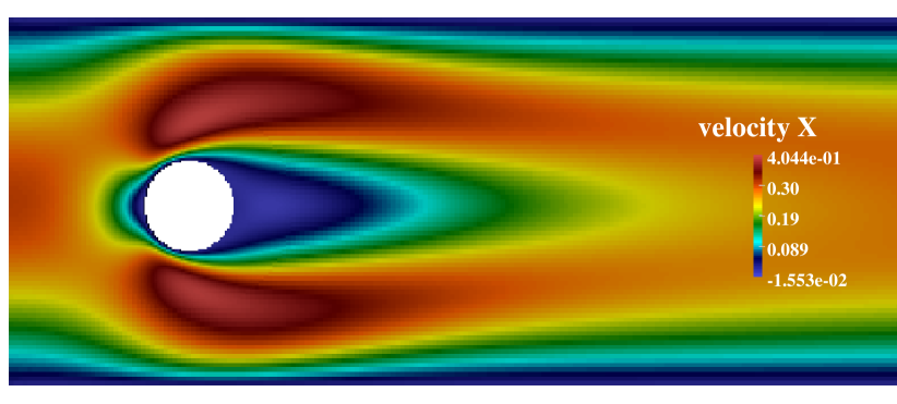
(a) $Re=20$

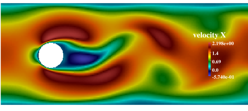
(b) $Re=100$

Figure 4: Velocity distribution for flow over cylinder at (a) $Re=20$ and (b) $Re=100$. The velocity magnitude is given by the color map.

Table 1: Simulation results of drag and lift coefficients, $c_{D}$ and $c_{L}$, for flow over cylinder at $Re=20,100$

	$Re=20$		$Re=100$
resolution	$c_{D}$	$c_{L}$	$c_{Dmax}$	$c_{Lmax}$	$St$
$D=40\Delta x_{L+1}$	5.745	0.01438	3.285	0.9751	0.3087
$D=80\Delta x_{L+1}$	5.664	0.01234	3.272	0.9934	0.3088
$D=160\Delta x_{L+1}$	5.621	0.01146	3.245	0.9888	0.3034
literature [45, 46, 6]	5.49-5.627	0.0092-0.0119	3.22-3.2650	0.9492-1.0709	0.295-0.3076

4.3 Flow over sphere at $Re=100$

The flow over sphere benchmark problem was chosen to validate our approach for the 3D case. Similar to the flow over cylinder, the flow phenomena can be categorized into different regimes based on the Reynolds number. Previous studies [47] have shown that the flow is steady and axisymmetric up to $Re\approx 210$. In the present study, the flow at $Re=100$ is chosen to evaluate the refinement mothod in three dimensions. The computational domain has a size of $[-15D,49D]\times[-15D,15D]\times[-15D,15D]$. Four levels of refinement are used, which are clusted around the sphere located at $\mathbf{x}=(0,0,0)$. Element size equals $\Delta x_{min}=D/32$ on the highest mesh level. The drag coefficients $c_{D}$ are defined the same as Eq. (4.2), where $A=\pi D^{2}/4$ for a sphere. The simulated results of $c_{D}$ and $Lr/D$ (normarlized recirculation length) are listed in Table 2 and in good agreement with those from the literature, proving the accurary of our approach in three dimensions.

Table 2: Simulation results of drag coefficients $c_{D}$ and normalized recirculation length $Lr/D$ for flow over sphere at $Re=100$

	$c_{D}$	$Lr/D$
present	1.090	0.872
literature [47, 48, 16]	1.06-1.098	0.863-0.880

5 Conclusion

In this paper, we presented a detailed LB implementation on non-uniform sparse octree data structure. Our method makes use of the strain rate information locally available to achieve quadratic interpolation for the velocity. This method requires only a minimum of four source elements from the adjecent level for both 2D and 3D, thus is highly efficient especially for paralization. To allow fluid elements to performance two consecutive advection steps, two layers of ghost elements are introduced at the mesh level interface and get filled up by interpolation during synchorous step. Two of the main implementation features are explained in details: weight based domain decomposition and level-wise elements arrangement. These are specially designed to improve efficiency in parallel simulations. Through the Taylor-Green vortex test case, the second order convergence was achieved for both velocity and strain rate. Moreover, laminar flow over cylinder in 2D and flow over sphere in 3D was investigated, where drag and lift coefficients, Strouhal number and recirculation length were calculated. Good agreement between simulation results and those from literature was observed, evidencing the accuracy of our method.

In the present study, region with mesh refinement was defined in the mesh generation step and fixed during flow simulation. The mesh adaptivity techniques are among our ongoing efforts. A dynamic load balancing algorithm was also under investigation to account for the altered mesh topology.

References

- [1] S. Chen, G. D. Doolen, Lattice boltzmann method for fluid flows, Annual review of fluid mechanics 30 (1) (1998) 329–364.
- [2] J. Bernsdorf, S. E. Harrison, S. M. Smith, P. V. Lawford, Concurrent numerical simulation of flow and blood clotting using the lattice boltzmann technique, International Journal of Bioinformatics Research and Applications 2 (4) (2006) 371–380.
- [3] C. K. Aidun, J. R. Clausen, Lattice-boltzmann method for complex flows, Annual Review of Fluid Mechanics 42 (2010) 439–472.
- [4] J. Zudrop, S. Roller, P. Asinari, Lattice boltzmann scheme for electrolytes by an extended maxwell-stefan approach, Physical Review E 89 (5) (2014) 053310.
- [5] T. Zeiser, G. Hager, G. Wellein, Benchmark analysis and application results for lattice boltzmann simulations on nec sx vector and intel nehalem systems, Parallel Processing Letters 19 (04) (2009) 491–511.
- [6] M. Schönherr, K. Kucher, M. Geier, M. Stiebler, S. Freudiger, M. Krafczyk, Multi-thread implementations of the lattice boltzmann method on non-uniform grids for cpus and gpus, Computers & Mathematics with Applications 61 (12) (2011) 3730–3743.
- [7] G. Eitel-Amor, M. Meinke, W. Schröder, A lattice-boltzmann method with hierarchically refined meshes, Computers & Fluids 75 (2013) 127–139.
- [8] M. Hasert, K. Masilamani, S. Zimny, H. Klimach, J. Qi, J. Bernsdorf, S. Roller, Complex fluid simulations with the parallel tree-based lattice boltzmann solver musubi, Journal of Computational Science 5 (5) (2014) 784–794.
- [9] O. Filippova, D. Hänel, Grid refinement for lattice-bgk models, Journal of Computational Physics 147 (1) (1998) 219–228.
- [10] C.-L. Lin, Y. G. Lai, Lattice boltzmann method on composite grids, Physical Review E 62 (2) (2000) 2219.
- [11] D. Yu, R. Mei, W. Shyy, A multi-block lattice boltzmann method for viscous fluid flows, International journal for numerical methods in fluids 39 (2) (2002) 99–120.
- [12] A. Dupuis, B. Chopard, Theory and applications of an alternative lattice boltzmann grid refinement algorithm, Physical Review E 67 (6) (2003) 066707.
- [13] J. Tölke, S. Freudiger, M. Krafczyk, An adaptive scheme using hierarchical grids for lattice boltzmann multi-phase flow simulations, Computers & Fluids 35 (8) (2006) 820–830.
- [14] D. Yu, S. S. Girimaji, Multi-block lattice boltzmann method: extension to 3d and validation in turbulence, Physica A: Statistical Mechanics and its Applications 362 (1) (2006) 118–124.
- [15] Y. Chen, Q. Kang, Q. Cai, D. Zhang, Lattice boltzmann method on quadtree grids, Physical Review E 83 (2) (2011) 026707.
- [16] G. Eitel-Amor, M. Meinke, W. Schröder, Lattice boltzmann simulations with locally refined meshes, in: 20th AIAA Computational Fluid Dynamics Conference, 2011, p. 3398.
- [17] D. Lagrava, O. Malaspinas, J. Latt, B. Chopard, Advances in multi-domain lattice boltzmann grid refinement, Journal of Computational Physics 231 (14) (2012) 4808–4822.
- [18] M. Hasert, H. Klimach, J. Bernsdorf, S. Roller, Aeroacoustic validation of the lattice boltzmann method on non-uniform grids, in: J. Eberhardsteiner (Ed.), European congress on computational methods in applied sciences and enginnering, 2012.
- [19] P. Neumann, T. Neckel, A dynamic mesh refinement technique for lattice boltzmann simulations on octree-like grids, Computational Mechanics 51 (2) (2013) 237–253.
- [20] A. Fakhari, T. Lee, Finite-difference lattice boltzmann method with a block-structured adaptive-mesh-refinement technique, Physical Review E 89 (3) (2014) 033310.
- [21] A. Fakhari, T. Lee, Numerics of the lattice boltzmann method on nonuniform grids: standard lbm and finite-difference lbm, Computers & Fluids 107 (2015) 205–213.
- [22] H. Chen, Volumetric formulation of the lattice boltzmann method for fluid dynamics: Basic concept, Physical Review E 58 (3) (1998) 3955.
- [23] H. Chen, O. Filippova, J. Hoch, K. Molvig, R. Shock, C. Teixeira, R. Zhang, Grid refinement in lattice boltzmann methods based on volumetric formulation, Physica A: Statistical Mechanics and its Applications 362 (1) (2006) 158–167.
- [24] M. Geier, A. Greiner, J. Korvink, Bubble functions for the lattice boltzmann method and their application to grid refinement, The European Physical Journal-Special Topics 171 (1) (2009) 173–179.
- [25] J. Tölke, M. Krafczyk, Second order interpolation of the flow field in the lattice boltzmann method, Computers & Mathematics with Applications 58 (5) (2009) 898–902.
- [26] M. Hasert, Multi-scale lattice boltzmann simulations on distributed octrees, Phd thesis, RWTH Aachen University (Oct 2013).
- [27] H. G. Klimach, M. Hasert, J. Zudrop, S. P. Roller, Distributed octree mesh infrastructure for flow simulations, in: J. Eberhardsteiner, H. J. Böhm, F. G. Rammerstorfer (Eds.), Proceedings of the 6th European Congress on Computational Methods in Applied Sciences and Engineering, 2012, p. 3390.
- [28] M. Hasert, J. Bernsdorf, S. Roller, Towards aeroacoustic sound generation by flow through porous media, Philosophical Transactions of the Royal Society A: Mathematical, Physical and Engineering Sciences 369 (1945) (2011) 2467–2475.
- [29] S. Zimny, B. Chopard, O. Malaspinas, E. Lorenz, K. Jain, S. Roller, J. Bernsdorf, A multiscale approach for the coupled simulation of blood flow and thrombus formation in intracranial aneurysms, Procedia Computer Science 18 (2013) 1006 – 1015.
- [30] J. Qi, M. Hasert, H. Klimach, S. Roller, Aeroacoustic simulation of flow through porous media based on lattice boltzmann method, in: Sustained Simulation Performance 2015, Springer, 2015, pp. 195–204.
- [31] A. Augier, F. Dubois, B. Graille, P. Lallemand, On rotational invariance of lattice boltzmann schemes, Computers & Mathematics with Applications 67 (2) (2014) 239–255.
- [32] G. Silva, V. Semiao, Truncation errors and the rotational invariance of three-dimensional lattice models in the lattice boltzmann method, Journal of Computational Physics 269 (2014) 259–279.
- [33] Y. Qian, D. d’Humières, P. Lallemand, Lattice bgk models for navier-stokes equation, EPL (Europhysics Letters) 17 (6) (1992) 479.
- [34] X. He, L.-S. Luo, M. Dembo, Some progress in lattice boltzmann method. part i. nonuniform mesh grids, Journal of Computational Physics 129 (2) (1996) 357–363.
- [35] M. Rheinländer, A consistent grid coupling method for lattice-boltzmann schemes, Journal of Statistical Physics 121 (1-2) (2005) 49–74.
- [36] A. J. Ladd, Numerical simulations of particulate suspensions via a discretized boltzmann equation. part 1. theoretical foundation, Journal of Fluid Mechanics 271 (1994) 285–309.
- [37] M. Junk, Z. Yang, Asymptotic analysis of lattice boltzmann outflow treatments, Communications in Computational Physics 9 (05) (2011) 1117–1127.
- [38] M. Bouzidi, M. Firdaouss, P. Lallemand, Momentum transfer of a Boltzmann-lattice fluid with boundaries, Physics of Fluids 13 (11) (2001) 3452–3459. doi:{10.1063/1.1399290}.
- [39] M. Schulz, M. Krafczyk, J. Tölke, E. Rank, Parallelization strategies and efficiency of cfd computations in complex geometries using lattice boltzmann methods on high-performance computers, in: M. Breuer, F. Durst, C. Zenger (Eds.), High performance scientific and engineering computing, Vol. 21, Springer, 2002, pp. 115–122.
- [40] C. Godenschwager, F. Schornbaum, M. Bauer, H. Köstler, U. Rüde, A framework for hybrid parallel flow simulations with a trillion cells in complex geometries, in: Proceedings of the International Conference on High Performance Computing, Networking, Storage and Analysis, ACM, 2013, p. 35.
- [41] G. M. Morton, A computer oriented geodetic data base and a new technique in file sequencing, Tech. rep., International Business Machines Company (1966).
- [42] M. E. Brachet, D. I. Meiron, S. A. Orszag, B. Nickel, R. H. Morf, U. Frisch, Small-scale structure of the taylor–green vortex, Journal of Fluid Mechanics 130 (1983) 411–452.
- [43] T. Krüger, F. Varnik, D. Raabe, Second-order convergence of the deviatoric stress tensor in the standard bhatnagar-gross-krook lattice boltzmann method, Physical Review E 82 (2) (2010) 025701.
- [44] M. Geier, M. Schönherr, A. Pasquali, M. Krafczyk, The cumulant lattice boltzmann equation in three dimensions: Theory and validation, Computers & Mathematics with Applications 70 (4) (2015) 507–547.
- [45] M. Schäfer, S. Turek, F. Durst, E. Krause, R. Rannacher, Benchmark computations of laminar flow around a cylinder, Springer, 1996.
- [46] B. Crouse, Lattice-boltzmann strömungssimulationen auf baumdatenstrukturen, Ph.D. thesis, Technische Universität München (2003).
- [47] T. Johnson, V. Patel, Flow past a sphere up to a reynolds number of 300, Journal of Fluid Mechanics 378 (1999) 19–70.
- [48] D. Hartmann, M. Meinke, W. Schröder, A strictly conservative cartesian cut-cell method for compressible viscous flows on adaptive grids, Computer Methods in Applied Mechanics and Engineering 200 (9) (2011) 1038–1052.