Abstract

In the present work we have searched the existence of the late time acceleration of the universe with string fluid as source of matter in anisotropic Heckmann-Suchking space-time by using 287 high red shift $(0.3\leq z\leq 1.4)$ SN Ia data of observed absolute magnitude along with their possible error from Union 2.1 compilation. It is found that the best fit values for $(\Omega_{m})_{0}$, $(\Omega_{\Lambda})_{0}$, $(\Omega_{\sigma})_{0}$ and $(q)_{0}$ are 0.2820, 0.7177, 0.0002 $\&$ -0.5793 respectively. Several physical aspects and geometrical properties of the model are discussed in detail.

Key words: String, SN Ia data, Heckmann-Suchking space-time.

1 Introduction

SN Ia observations (Riess et al. 1998; Perlmutter et al. 1999) confirmed that the observable universe is undergoing an accelerated expansion. This acceleration is realized due to unknown cosmic fluid - dark energy (DE) which have positive energy density and negative pressure. So, it violate the strong energy condition (SEC). The authors of ref. [3] confirmed that the violation of SEC gives anti gravitational effect that provides an elegant description of transition of universe from deceleration zone to acceleration zone. In the literature, cosmological constant is the simplest candidate to describe the present acceleration of universe (GrØn and Hervik 2007) but it suffers two problems - the fine tunning and cosmic coincidence problems (Carroll et al. 1992, Copeland et al. 2006). In the early of 21 century, some authors (Copeland et al. 2006, Alam et al. 2003) have developed few scalar field DE models, namely the phantom, quintessence and k-essence rather than positive $\Lambda$. In the physical cosmology, the dynamical form of DE with an effective equation of state (EOS), $\omega<-\frac{1}{3}$, were proposed instead of positive $\Lambda$ (Komastu et al. 2009, Riess et al. 2004, Astier et al. 2006).

The substantial theoretical progress in string theory has brought forth a diverse new generation of cosmological models, some of which are subject to direct observational tests. Firstly the gravitational effect of cosmic strings are investigated by Letelier (1979, 1983). The present day observations of universe indicate the existence of large scale network of strings in early universe (Kible, 1976, 1980). Recently, Pradhan et al. (2007) and Yadav et al. (2009) have studied string cosmological model in non-homogeneous space-time in which geometric strings were considered as source of matter. After the big bang, the universe may have undergone so many phase transitions as its temperature cooled below some critical temperature as suggested by grand unified theories (Zel’dovich et al. 1975; Kibble 1976, 1980; Everett 1981; Vilenkin 1981). At the very early stage of evolution of universe, the symmetry of universe was broken spontaneously that rises some topologically-stable defects such as domain walls, strings and monopoles (Vilenkin 1981, 1985). Among all the three cosmological structures, only strings give rise the density perturbations that leads the formation of galaxies. Pogosian et al. (2003, 2006) have suggested that the cosmic strings are not responsible for CMB fluctuations and observed clustering of galaxies. In 2011, Pradhan and Amirhashchi (2011) have considered time varying scale factor that generates a transitioning universe in Bianchi -V space-time. Yadav et al. (2011) and Bali (2008) have obtained Bianchi-V string cosmological models in general relativity. The magnetized string cosmological models are discussed by some authors (Chakraborty 1980; Tikekar and Patel 1992, 1994; Patel and Maharaj 1996; Singh and Singh 1999; Saha and Visineusu 2008) in different physical contexts. Recently Goswami et al (2015) have studied $\Lambda$CDM cosmological model in absence of string. In this paper we have established the existence of string cosmological model in anisotropic Hecmann-Suchuking space-time.The organization of the paper is as follows: The model and field equations are presented in section 2. In Section 3, 4 $\&$ 5 we obtain the expressions for Hubble constant, Luminosity distance and apparent magnitude. Section 6 deals the estimation of present values of energy parameters. Finally the conclusions of the paper are presented in section 7.

2 The Model and Field equations

We consider a general Heckmann-Schucking metric

$$ds^{2}=c^{2}dt^{2}-A^{2}dx^{2}-B^{2}dy^{2}-C^{2}dz^{2}$$ (1)

where A, B and C are functions of time only.
The energy-momentum tensor for a cloud of massive strings and perfect fluid distribution is taken as

$$T_{ij}=(p+\rho)u_{i}u_{j}-pg_{ij}-\lambda x^{i}x^{j}$$ (2)

with

$$g_{ij}u^{i}u^{j}=1$$ (3)

and

$$x^{i}x^{i}=-1,u^{i}x_{i}=0$$ (4)

where $u^{i}$ is the four velocity vector, $\rho$ is the rest energy density of the system of strings,  $\lambda$ is the tension density of the strings and  $x^{i}$ is a unit space-like vector representing the direction of strings.
In co-moving co-ordinates,

$$u^{\alpha}=0,\alpha=1,2or3.$$ (5)

Choosing $x^{i}$ parallel to $\partial/\partial x$, we have

$$x^{i}=(A^{-1},0,0,0).$$ (6)

If the particle density of the configuration is denoted by $\rho_{m}$, then

$$\rho=\rho_{m}+\lambda$$ (7)

The Einstein field equations are

$$R_{ij}-\frac{1}{2}Rg_{ij}+\Lambda g_{ij}=-\frac{8\pi G}{c^{4}}T_{ij}$$ (8)

Choosing co-moving coordinates,the field equations (8) in terms of line element (1) can be written as

$$\frac{B_{44}}{B}+\frac{C_{44}}{C}+\frac{B_{4}C_{4}}{BC}=-\frac{8\pi G}{c^{2}}(p-\lambda)+\Lambda c^{2}$$ (9)

$$\frac{A_{44}}{A}+\frac{C_{44}}{C}+\frac{A_{4}C_{4}}{AC}=-\frac{8\pi G}{c^{2}}p+\Lambda c^{2}$$ (10)

$$\frac{A_{44}}{A}+\frac{B_{44}}{C}+\frac{A_{4}B_{4}}{AB}=-\frac{8\pi G}{c^{2}}p+\Lambda c^{2}$$ (11)

$$\frac{A_{4}B_{4}}{AB}+\frac{B_{4}C_{4}}{BC}+\frac{C_{4}A_{4}}{AC}=\frac{8\pi G}{c^{2}}\rho+\Lambda c^{2}$$ (12)

where $A_{4}$,$B_{4}$ and $C_{4}$ stand for time derivatives of A,B,C respectively. the mass-energy conservation equation $T^{ij}_{;j}=0$ gives

$$\rho_{4}+(p+\rho)(\frac{A_{4}}{A}+\frac{B_{4}}{B}+\frac{C_{4}}{C})-\lambda\frac{A_{4}}{A}=0$$ (13)

Where $A_{4}$,$B_{4}$ and $C_{4}$ stand for time derivatives of A,B and C respectively. Subtracting (10) from (9),(11) from (10) and (11) from (9) we get

$$\frac{A_{44}}{A}-\frac{B_{44}}{B}+\frac{A_{4}C_{4}}{AC}-\frac{B_{4}C_{4}}{BC}=-\frac{8\pi G}{c^{2}}\lambda$$ (14)

$$\frac{B_{44}}{B}-\frac{C_{44}}{C}+\frac{A_{4}B_{4}}{AB}-\frac{A_{4}C_{4}}{AC}=0$$ (15)

$$\frac{C_{44}}{C}-\frac{A_{44}}{A}+\frac{B_{4}C_{4}}{BC}-\frac{A_{4}B_{4}}{AB}=\frac{8\pi G}{c^{2}}\lambda$$ (16)

Subtracting(16) from (14), we get

$$\frac{B_{44}}{B}+\frac{C_{44}}{C}+\frac{2B_{4}C_{4}}{BC}=2\frac{A_{44}}{A}+\frac{A_{4}C_{4}}{AC}+\frac{A_{4}B_{4}}{AB}+\frac{16\pi G}{c^{2}}\lambda$$

This equation can be re-written in the following form

$$\biggl{(}\frac{(BC)_{4}}{BC}\biggr{)}_{4}+\biggl{(}\frac{(BC)_{4}}{BC}\biggr{)}^{2}=2\biggl{(}\frac{A_{4}}{A}\biggr{)}_{4}+2\frac{A^{2}_{4}}{A^{2}}+\frac{A_{4}(BC)_{4}}{ABC}+\frac{16\pi G}{c^{2}}\lambda$$

This is simplified as

$$\biggl{(}\frac{(BC)_{4}}{BC}-2\frac{A_{4}}{A}\biggr{)}_{4}+\biggl{(}\frac{(BC)_{4}}{BC}-2\frac{A_{4}}{A}\biggr{)}\frac{(ABC)_{4}}{ABC}=\frac{16\pi G}{c^{2}}\lambda$$ (17)

This equation suggests the following relation ship among A B and C

$$A^{n}=BC$$ (18)

where $n\neq 2$, otherwise $\lambda$ would be zero. We can assume

$$B=A^{n/2}D\&C=A^{n/2}D^{-1},D=D(t)$$ (19)

Further integrating equation (15), we get the first integral

$$\frac{D_{4}}{D}=\frac{K}{A^{n+1}}$$ (20)

Where K is an arbitrary constant of integration. Equation(13) simplifies as

$$\rho_{4}+(n+1)\frac{A_{4}}{A}(p+\rho)-\lambda\frac{A_{4}}{A}=0$$

Using equation(7), this becomes

$$(\rho_{m})_{4}+(n+1)\frac{A_{4}}{A}(\rho_{m}+p)+\lambda_{4}+n\frac{A_{4}}{A}\lambda=0$$ (21)

If matter and string tension co-exist without much interaction , this equation splits into two parts.

$$(\rho_{m})_{4}+(n+1)\frac{A_{4}}{A}(\rho_{m}+p)=0$$ (22)

$\&$

$$\lambda_{4}+n\frac{A_{4}}{A}\lambda=0$$ (23)

This gives following expression for matter density $\rho_{m}$ and string tension $\lambda$ for p=0(dust filled universe)

$$\rho_{m}=\frac{(\rho_{m})_{0}(A)^{n+1}_{0}}{A^{n+1}}$$ (24)

and

$$\lambda=\frac{(\lambda)_{0}(A)^{n}_{0}}{A^{n}}$$ (25)

The Hubble’s constant in this model is

$$H=u^{i}_{;i}=\frac{1}{3}(\frac{A_{4}}{A}+\frac{B_{4}}{B}+\frac{C_{4}}{C})=\frac{(n+1)}{3}\frac{A_{4}}{A}$$ (26)

Equations (9)-(12) and (20) are simplified as

$$\frac{n+2}{2}\frac{A_{44}}{A}+\frac{n^{2}}{4}\frac{A^{2}_{4}}{A^{2}}=-\frac{8\pi G}{c^{2}}\Bigl{(}p-\frac{\Lambda c^{4}}{8\pi G}+\frac{K^{2}c^{2}}{8\pi GA^{2(n+1)}}\Bigr{)}$$ (27)

$$\frac{A_{44}}{A}+n\frac{A^{2}_{4}}{A^{2}}=\frac{16\pi G}{c^{2}}\frac{\lambda}{n-2}$$ (28)

$$\frac{n(n+4)}{4}\frac{A^{2}_{4}}{A^{2}}=\frac{K^{2}}{A^{2(n+1)}}+\frac{8\pi G}{c^{2}}\rho+\Lambda c^{2}$$ (29)

We see from equation(28) that  $\lambda$=0 for   n=2 and other equations convert to the Einstein’s field equations of LRS Bianchi type I model for perfect fluid without string
The average scale factor ’a’ of LRS Bianchi type I model is defined as

$$a=(ABC)^{1/3}=A^{\frac{n+1}{3}}$$ (30)

The spatial volume ’V’ is given by

$$V=a^{3}=ABC=A^{n+1}$$ (31)

Equations(27)-(29) can be re-written as

$$\frac{n(n+4)}{2(n+1)}\Bigl{(}\frac{A_{44}}{A}+\frac{n-1}{2}\frac{A^{2}_{4}}{A^{2}}\Bigr{)}=-\frac{8\pi G}{c^{2}}\Bigl{(}p-\frac{\lambda}{n+1}+\frac{K^{2}c^{2}}{8\pi GA^{2(n+1)}}-\frac{\Lambda c^{4}}{8\pi G}\Bigr{)}$$ (32)

$$H^{2}=\frac{4(n+1)^{2}}{9n(n+4)}\frac{8\pi G}{c^{2}}\Bigl{(}\rho_{m}+\lambda+\frac{\Lambda c^{4}}{8\pi G}+\frac{K^{2}c^{2}}{8\pi GA^{2(n+1)}}\Bigr{)}$$ (33)

We now assume that the string tension $\lambda$, cosmological constant $\Lambda$ and the term due to anisotropy also act like energies with densities and pressures as

$$\rho_{\lambda}=\lambda\hskip 7.22743pt\rho_{\Lambda}=\frac{\Lambda c^{4}}{8\pi G}\hskip 36.135pt\rho_{\sigma}=\frac{K^{2}c^{2}}{8\pi GA^{2(n+1)}}$$

$$p_{\lambda}=-\frac{\lambda}{n+1}\hskip 7.22743ptp_{\Lambda}=-\frac{\Lambda c^{4}}{8\pi G}\hskip 36.135ptp_{\sigma}=\frac{K^{2}c^{2}}{8\pi GA^{2(n+1)}}$$

(34)

It can be easily verified that energy conservation laws (22) $\&$ (23) holds separately for $\rho_{\Lambda}$, $\rho_{\sigma}$ $\&$ $\rho_{\lambda}$

$$(\rho_{\Lambda})_{4}+3H(p_{\Lambda}+\rho_{\Lambda})=0,~{}(\rho_{\sigma})_{4}+3H(p_{\sigma}+\rho_{\sigma})=0~{}\&~{}(\rho_{\lambda})_{4}+3H(p_{\lambda}+\rho_{\lambda})=0$$

(35)

The equations of state for matter, $\lambda$, $\sigma$ and $\Lambda$ energies are as follows

$$p_{m}=\omega_{m}\rho_{m}$$

$$p_{\lambda}=\omega_{\lambda}\rho_{\lambda}\because p_{\lambda}=-\frac{1}{n+1}\rho_{\lambda}\therefore\omega_{\lambda}=-\frac{1}{n+1}$$

$$p_{\Lambda}=\omega_{\Lambda}\rho_{\Lambda}\because p_{\Lambda}+\rho_{\Lambda}=0\therefore\omega_{\Lambda}=-1$$

$$\because p_{\sigma}=\rho_{\sigma}\therefore\omega_{\sigma}=1$$

(36)

where $\omega_{m}$=0 for matter in form of dust, $\omega_{m}=\frac{1}{3}$ for matter in form of radiation. There are certain more values of $\omega_{m}$ for matter in different forms during the coarse of evolution of the universe. Now we use the following relation between scale factor a and red shift z

$$\frac{a_{0}}{a}=(\frac{A_{0}}{A})^{\frac{n+1}{3}}=1+z$$ (37)

The suffix(0) is meant for the value at present time.The energy density $\rho$ comprises of following components

$$\rho=\bigl{(}\rho_{m}+\rho_{\lambda}+\rho_{\Lambda}+\rho_{\sigma}\bigr{)}$$ (38)

Integrations of energy equations(35) yield

$$\rho_{i}=(\rho_{i})_{0}(1+z)^{3(1+\omega_{i})}\therefore\rho=\sum_{i}(\rho_{i})_{0}(1+z)^{3(1+\omega_{i})}$$

(39)

where suffix i corresponds to various energies densities. We write equations (32) and (33) as

$$\frac{n(n+4)}{2(n+1)}\Bigl{(}\frac{A_{44}}{A}+\frac{n-1}{2}\frac{A^{2}_{4}}{A^{2}}\Bigr{)}=-\frac{8\pi G}{c^{2}}\Bigl{(}p_{m}+p_{\lambda}+p_{\Lambda}+p_{\sigma}\Bigr{)}$$ (40)

$$H^{2}=\frac{4(n+1)^{2}}{9n(n+4)}\frac{8\pi G}{c^{2}}\bigl{(}\rho_{m}+\rho_{\lambda}+\rho_{\Lambda}+\rho_{\sigma}\bigr{)}$$ (41)

3 Dust filled universe

The present stage of the universe is full of dust for which pressure $p_{m}=0$. We define critical density $\rho_{c}$ as

$$\rho_{c}=\frac{9n(n+4)c^{2}H^{2}}{32(n+1)^{2}\pi G}$$ (42)

Then (41) gives

$$\Omega_{m}+\Omega_{\lambda}+\Omega_{\Lambda}+\Omega_{\sigma}=1$$ (43)

Where

$$\Omega_{m}=\frac{\rho_{m}}{\rho_{c}}=\frac{(\Omega_{m})_{0}H^{2}_{0}(1+z)^{3}}{H^{2}},\Omega_{\lambda}=\frac{\rho_{\lambda}}{\rho_{c}}=\frac{(\Omega_{\lambda})_{0}H^{2}_{0}(1+z)^{\frac{3n}{n+1}}}{H^{2}}$$

$$\Omega_{\Lambda}=\frac{\rho_{\Lambda}}{\rho_{c}}=\frac{(\Omega_{\Lambda})_{0}H^{2}_{0}}{H^{2}},\Omega_{\sigma}=\frac{\rho_{\sigma}}{\rho_{c}}=\frac{(\Omega_{\sigma})_{0}H^{2}_{0}(1+z)^{6}}{H^{2}}$$

(44)

3.1 Expression for Hubble’s Constant

Adding all the three above and using (43), we get expression for Hubble’s constant

$$H^{2} = H^{2}_{0}\sum_{i}(\Omega_{i})_{0}(1+z)^{3(1+\omega_{i})}$$

$$= H^{2}_{0}\bigl{[}(\Omega_{m})_{0}(1+z)^{3}+(\Omega_{\lambda})_{0}(1+z)^{\frac{3n}{n+1}}+(\Omega_{\sigma})_{0}(1+z)^{6}+(\Omega_{\Lambda})_{0}\bigr{]}$$

$$= H^{2}_{0}\bigl{[}(\Omega_{m})_{0}(\frac{A_{0}}{A})^{n+1}(\Omega_{\lambda})_{0}(\frac{A_{0}}{A})^{n}+(\Omega_{\sigma})_{0}(\frac{A_{0}}{A})^{2(n+1)}+(\Omega_{\Lambda})_{0}\bigr{]}$$

(45)

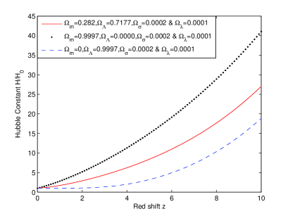
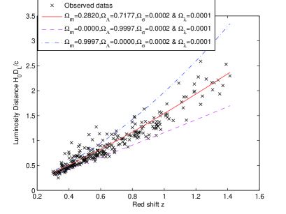
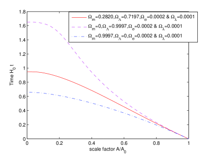
Figure 1: Variation of $\frac{H}{H_{0}}$, $m$, $\frac{H_{0}D_{L}}{c}$, $q$, $H_{0}t$ and $\sigma$ with redshift.

Now we present two graphs on the basis of above equation(see fig. 1 & fig. 2).

These figures show that Hubble’s constant increases over red shift. We can say that Hubble’s constant decreases over time. We also notice from fig. 1 that in the case lambda dominated universe ($(\Omega_{m})_{0}$=0 or .2820 ) Hubble’s constant vary slowly over time in comparison to matter dominated universe($\Omega_{\Lambda}=0$).

4 Luminosity Distance verses Red Shift Relation

If x be the spatially coordinate distance of a source with red shift z from us, the luminosity distance which determines flux of the source is given by

$$D_{L}=A_{0}x(1+z)$$ (46)

Geodesic for metric (1) ensures that if in the beginning

$$\frac{dy}{ds}=0and\frac{dz}{ds}=0$$

then

$$\frac{d^{2}y}{ds^{2}}=0and\frac{d^{2}z}{ds^{2}}=0$$

So if a particle moves along x- direction, it continues to move along x- direction always.If we assume that line of sight of a vantage galaxy from us is along x-direction then path of photons traveling through it satisfies

$$ds^{2}=c^{2}dt^{2}-A^{2}dx^{2}=0$$

From this we obtain

$$x = \int^{x}_{0}dx=\int^{t_{0}}_{t}\frac{dt}{A(t)}=\frac{1}{A_{0}H_{0}}\int^{z}_{0}\frac{dz}{(1+z)^{\frac{n-2}{n+1}}h(z)}$$

$$= \frac{1}{A_{0}H_{0}}\int^{z}_{0}\frac{dz}{(1+z)^{\frac{n-2}{n+1}}\sqrt{\bigl{[}(\Omega_{m})_{0}(1+z)^{3}+(\Omega_{\lambda})_{0}(1+z)^{\frac{3n}{n+1}}+(\Omega_{\sigma})_{0}(1+z)^{6}+(\Omega_{\Lambda})_{0}\bigr{]}}}$$

(47)

Where we have used $dt=dz/\dot{z}$ and from eqns (26) and (37)

$$\dot{z}=-H(1+z)~{}\&~{}h(z)=\frac{H}{H_{0}}$$

.
So the luminosity distance is given by

$$D_{L}=\frac{c(1+z)}{H_{0}}\int^{z}_{0}\frac{dz}{(1+z)^{\frac{n-2}{n+1}}\sqrt{\bigl{[}(\Omega_{m})_{0}(1+z)^{3}+(\Omega_{\lambda})_{0}(1+z)^{\frac{3n}{n+1}}+(\Omega_{\sigma})_{0}(1+z)^{6}+(\Omega_{\Lambda})_{0}\bigr{]}}}$$ (48)

5 Apparent Magnitude verses Red Shift relation for Type Ia supernova’s(SN Ia):

The Absolute and Apparent magnitude of a source (M and m) are related to the red shift of the source by following relation

$$m-M=5log_{10}\bigl{(}\frac{D_{L}}{Mpc}\bigr{)}+25$$ (49)

The Type Ia supernova (SN Ia) can be observed when white dwarf stars exceed the mass of the Chandrasekhar limit and explode. The belief is that SN Ia are formed in the same way irrespective of where they are in the universe, which means that they have a common absolute magnitude M independent of the red shift z. Thus they can be treated as an ideal standard candle. We can measure the apparent magnitude m and the red shift z observationally, which of course depends upon the objects we observe.
To get absolute Magnitude M of a supernova, we consider supernova at very small red shift. Let us consider a supernova 1992P at low-red shift z = 0.026 with m = 16.08.For low red shift supernova,we have the following relation

$$D_{L}=\frac{cz}{H_{0}}$$ (50)

Putting values z = 0.026, m = 16.08 and $D_{L}$ from (50),
Equation (49) gives M for all SN Ia as follows.

$$M=5log_{10}\bigl{(}\frac{H_{0}}{.026c}\bigr{)}-8.92$$ (51)

From equations (49) and (51)

$$log_{10}(H_{0}D_{L})=(m-16.08)/5+log_{10}(.026cMpc)$$ (52)

The equation(52) gives observed value of Luminosity distance in term of observed value of apparent magnitude whereas the equation (48) gives the theoretically value of luminosity distance in terms of red shift on the basis of our model. Next, from equations (52) and (48) we get the following expression for (m,z) relations of Supernova’s SN Ia.

$$m=16.08+\\ 5log_{10}\Bigl{(}\frac{1+z}{.026}\Bigr{)}\times$$

$$\int^{z}_{0}\frac{dz}{(1+z)^{\frac{n-2}{n+1}}\sqrt{\bigl{[}(\Omega_{m})_{0}(1+z)^{3}+(\Omega_{\lambda})_{0}(1+z)^{\frac{3n}{n+1}}+(\Omega_{\sigma})_{0}(1+z)^{6}+(\Omega_{\Lambda})_{0}\bigr{]}}}$$ (53)

6 Estimation of Present values of Energy parameters $(\Omega_{m})_{0},(\Omega_{\Lambda})_{0},(\Omega_{\lambda})_{0}~{}\&~{}(\Omega_{\sigma})_{0}$

String tension play important role in the study of early evolution of the universe. We also notice that after publication of WMAP data, today there is considerable evidence in support of anisotropic model of universe. In the past, there might had been certain anisotropies in the universe . Our model validates that both string tension as well as anisotropy decreases over time. Considering it, we give very low present values to $(\Omega_{\sigma})_{0}$ and $(\Omega_{\lambda})_{0}$. In our earlier work we developed models with n = 2 which make string tension $\lambda$=0. So we take

$$n=2.1,(\Omega_{\sigma})_{0}=.0002\&(\Omega_{\lambda})_{0}=.0001$$ (54)

in our present model. Now we present two Tables(See Appendix-1 and 2) which contain $287$ high red shift ($0.3\leq z\leq 1.4$ ) SN Ia supernova data of observed apparent magnitude and luminosity distances along with their possible error from Union $2.1$ compilation. These Tables also contains the corresponding theoretical values of apparent magnitudes and luminosity distances for $\Omega_{m}$ = $0.2820$, $0$ and $1$ respectively which are obtained as per from Equation(48) and (52). As stated in the introduction, our purpose is to obtain the results close to WMAP on the basis of union 2.1 compilations for our model, so we have obtained the various sets of theoretical data’s of apparent magnitudes and luminosity distances corresponding to different values of $\Omega_{m}$ in between $0$ to $1$. In order to see that out of the these sets of theoretical data’s of apparent magnitudes and luminosity distances which one is close to the observational values, we calculate $\chi^{2}$ using following formula due to Amanullah et al.(2010). The tables[1] and [2] describe the various values of $\chi^{2}$ against values of $\Omega_{m}$ ranging in between $0$ to $1$.

$\chi_{SN}^{2}=A-\frac{B^{2}}{C}+log_{10}(\frac{C}{2\pi})$

Where

$A=\overset{60}{\underset{i=1}{\sum}}\frac{\left[\left(m\right)_{ob}-\left(m\right)_{th}\right]^{2}}{\sigma_{i}^{2}}$

$B=\overset{60}{\underset{i=1}{\sum}}\frac{\left[\left((m\right)_{ob}-\left((m\right)_{th}\right]}{\sigma_{i}^{2}}$

And

$C=\overset{60}{\underset{i=1}{\sum}}\frac{1}{\sigma_{i}^{2}}$

(55)

$(\Omega_{m)_{0}}$	$\chi_{SN}^{2}$	$\chi_{SN}^{2}/287$
0	5462.2	19.03205575
0.1	4972.8	17.32682927
0.2	4822.8	16.80418118
0.21	4816.5	16.78222997
0.26	4800.2	16.72543554
0.27	4799.4	16.72264808
0.28	4799.3	16.72229965
0.28	4799.3	16.72229965
0.281	4799.3	16.72229965
0.282	4799.3	16.72229965
0.283	4799.4	16.72264808
0.29	4799.8	16.72404181
0.3	4800.9	16.72787456
0.9997	5312.2	18.50940767

Table 1 : $\chi^{2}$ table for best fitting theoretical and observed values of apparent magnitudes‘m’

$(\Omega_{m)_{0}}$	$\chi_{SN}^{2}$	$\chi_{SN}^{2}/287$
0	223.1983	0.777694425
0.1	203.6246	0.70949338
0.2	197.6239	0.688585017
0.21	197.3738	0.687713589
0.26	196.7195	0.685433798
0.27	196.6878	0.685323345
0.28	196.6836	0.685308711
0.281	196.6836	0.685308711
0.282	196.6836	0.685308711
0.283	196.6874	0.685321951
0.29	196.7049	0.685382927
0.3	196.7499	0.685539721
0.9997	217.2009	0.756797561

Table 2 : $\chi^{2}$ table for best fitting theoretical and observed values of luminosity distance$D_{L}$

The above tables depict the fact that the best fit values of $\Omega_{m}$ and therefore $\Omega_{\Lambda}$ are as follows

$$\Omega_{m}=0.2820~{}~{}\&~{}~{}\Omega_{\Lambda}=0.7177$$ (56)

6.1 Deceleration Parameter

The deceleration parameter is given by

$$q=-\frac{aa_{44}}{a_{4}^{2}}=-\frac{n-2}{n+1}-\frac{3}{n+1}\frac{AA_{44}}{A_{4}^{2}}$$

From equations (39)-(53)

$$\frac{AA_{44}}{A^{2}_{4}} = -\frac{n+1}{2}\sum_{i}\omega_{i}\Omega_{i}-\frac{n-1}{2}$$

$$= -\frac{n+1}{2}(-\Omega_{\Lambda}-\frac{1}{n+1}\Omega_{\lambda}+\Omega_{\sigma})-\frac{n-1}{2}$$

$$\therefore q = \frac{3}{2}\frac{(-(\Omega_{\Lambda})_{0}-\frac{1}{n+1}(\Omega_{\lambda})_{0}(1+z)^{\frac{3n}{n+1}}+(\Omega_{\sigma})_{0}(1+z)^{6})}{\bigl{[}(\Omega_{m})_{0}(1+z)^{3}+(\Omega_{\lambda})_{0}(1+z)^{\frac{3n}{n+1}}+(\Omega_{\sigma})_{0}(1+z)^{6}+(\Omega_{\Lambda})_{0}\bigr{]}}+\frac{1}{2}$$

(57)

$$At~{}~{}z=0.7170,~{}~{}q=-0.0004~{}~{}\&~{}~{}at~{}~{}z=0.7180,~{}~{}q=.0002$$

So the universe entered the accelerating phase at $z\thicksim 0.7175\backsimeq t\thicksim 0.4616H^{-1}_{0}\thicksim 6.27\times 10^{9}yrs$ in the past before as from now.
The present value of q is

$$q_{0}=-0.5793$$

This equation clearly show that without presence of $\Lambda$ term in the Einstein’s field equation(8), one can’t imagine of accelerating universe.This equation also expresses the fact that anisotropy raises the lower limit value of $(\Omega_{\Lambda})_{0}$ required for acceleration at present. This may be seen in the following way.
For isotropic model(FRW) acceleration requires

$$(\Omega_{\Lambda})_{0}\geq.33$$ (58)

For anisotropic model with out string

$$(\Omega_{\Lambda})_{0}\geq.33+(\Omega_{\sigma})_{0}=.3302$$ (59)

For anisotropic model with string

$$(\Omega_{\Lambda})_{0}\geq.3559+(\Omega_{\sigma})_{0}-.0123(\Omega_{\lambda})_{0}=.3360$$ (60)

6.2 Age of the Universe

The present age of the universe is obtained as follows

$$t_{0} = \int^{t_{0}}_{0}dt=\int^{\infty}_{0}\frac{dz}{H(1+z)}$$

$$= \int^{\infty}_{0}\frac{dz}{H_{0}(1+z)\sqrt{\bigl{[}(\Omega_{m})_{0}(1+z)^{3}+(\Omega_{\lambda})_{0}(1+z)^{\frac{3n}{n+1}}+(\Omega_{\sigma})_{0}(1+z)^{6}+(\Omega_{\Lambda})_{0}\bigr{]}}}$$

$$= \int^{\infty}_{0}\frac{3dA}{(n+1)H_{0}A\sqrt{\bigl{[}(\Omega_{m})_{0}(\frac{A_{0}}{A})^{(n+1)}+(\Omega_{\lambda})_{0}(\frac{A_{0}}{A})^{n}+(\Omega_{\sigma})_{0}(\frac{A_{0}}{A})^{2(n+1)}+(\Omega_{\Lambda})_{0}\bigr{]}}}$$

(61)

Where we have used $dt=dz/\dot{z}$ and $\dot{z}=-H(1+z)$
We see that at large red-shift, $H_{0}t$ becomes constant and it tends to the value $0.9505$. So the Present age of the universe as per our model is

$$t_{0}=0.9505H^{-1}_{0}=13.2799\times 10^{9}years$$ (62)

6.3 Densities of the various Energies in the universe :

The energy density is given by (39)

$$\rho_{i}=(\Omega_{i})_{0}(\rho_{c})_{0}(1+z)^{3(1+\omega_{i})}$$

$$\therefore\rho=\sum_{i}(\Omega_{i})(\rho_{c})_{0}(1+z)^{3(1+\omega_{i})}$$

(63)

where i stands for various types of energies such as matter energy, dark energy,energies due to anisotropy of the universe and string tension. Taking,n=2.1,$\Omega_{m}=0.2820,\Omega_{\Lambda}=0.7177,\Omega_{\sigma}=0.0002\&\Omega_{\lambda}=0.0001$ , $H_{0}=72km/sec./Mpc$,$h_{0}\backsimeq.72$ $G=6.6720e-008cm^{3}/sec^{2}/gm$

$$(\rho_{c})_{0}=\frac{9n(n+4)c^{2}H_{0}^{2}}{32(n+1)^{2}\pi G}=1.8795h^{2}_{0}\times 10^{-29}gm/cm^{3}$$ (64)

The dust energy and its current value for flat universe is given as

$$(\rho_{m})=(\Omega_{m})_{0}(\rho_{c})_{0}(1+z)^{3},~{}\&~{}(\rho_{m})_{0}=.5262h^{2}_{0}\times 10^{-29}gm/cm^{3}$$ (65)

dark energy $(\rho_{\Lambda})$ and its current value is given as

$$(\rho_{\Lambda})=(\rho_{\Lambda})_{0}=1.35268h^{2}_{0}\times 10^{-29}gm/cm^{3}$$ (66)

The string tension $\lambda$ and its current value is given as

$$\lambda=(\Omega_{\lambda})_{0}(\rho_{c})_{0}(1+z)^{2.0323}~{}\&~{}(\lambda)_{0}=(\rho_{\lambda})_{0}=0.00018h^{2}_{0}\times 10^{-29}gm/cm^{3}$$ (67)

And finally anisotropy $\rho_{\sigma}$ and its current value is given as

$$(\rho_{\sigma})=(\Omega_{\sigma})_{0}(\rho_{c})_{0}(1+z)^{6}~{}\&~{}(\rho_{\sigma})_{0}=0.00036h^{2}_{0}\times 10^{-29}gm/cm^{3}$$ (68)

6.4 Shear Scalar($\sigma$), Relative Anisotropy($\sigma^{2}/\rho_{m}$) & Mean Anisotropy Parameter ($A_{m}$)

The shear scalar($\sigma$), relative anisotropy($\sigma^{2}/\rho_{m}$) & the mean anisotropy parameter ($A_{m}$)are defined as and are given by

$$\sigma^{2} = \frac{1}{2}(\overset{3}{\underset{i=1}{\sum}}H_{i}^{2}-3\theta^{2})$$

$$= \frac{(n-2)^{2}}{12}\frac{A^{2}_{4}}{A^{2}}+\frac{D^{2}_{4}}{D^{2}}$$

$$\sigma = H_{0}\sqrt{\frac{3(n-2)^{2}}{4(n+1)^{2}}\bigl{[}(\Omega_{m})_{0}(1+z)^{3}+(\Omega_{\lambda})_{0}(1+z)^{\frac{3n}{n+1}}+(\Omega_{\Lambda})_{0}\bigr{]}+3(\Omega_{\sigma})_{0}(1+z)^{6}}$$

(69)

$$\frac{\sigma^{2}}{\rho_{m}}=\frac{H^{2}_{0}\big{(}\frac{3(n-2)^{2}}{4(n+1)^{2}}\bigl{[}(\Omega_{m})_{0}(1+z)^{3}+(\Omega_{\lambda})_{0}(1+z)^{\frac{3n}{n+1}}+(\Omega_{\Lambda})_{0}\bigr{]}+3(\Omega_{\sigma})_{0}(1+z)^{6}\bigr{)}}{(\Omega_{m})_{0}(\rho_{c})_{0}(1+z)^{3}}$$ (70)

$$A_{m} = \frac{1}{3}\overset{3}{\underset{i=1}{\sum}}(\frac{H_{i}-H}{H})^{2}$$

$$= \frac{(n-2)^{2}}{2(n+1)^{2}}+\frac{6A^{2}D_{4}^{2}}{(n+1)^{2}D^{2}A^{2}_{4}}$$

$$= \frac{(n-2)^{2}}{2(n+1)^{2})}+\frac{3n(n+4)}{2(n+1)^{2}}\frac{(\Omega_{\sigma})_{0}(1+z)^{6}}{\bigl{[}(\Omega_{m})_{0}(1+z)^{3}+(\Omega_{\lambda})_{0}(1+z)^{\frac{3n}{n+1}}+(\Omega_{\sigma})_{0}(1+z)^{6}+(\Omega_{\Lambda})_{0}\bigr{]}}$$

(71)

where $H_{i}(i=1,2,3)$ represent the directional Hubble parameters in the direction of x,y and z , respectively.
The present value of shear scalar is given as

$$(A_{m})_{0}=0.38107518$$

The present value of mean anisotropy parameter $A_{m}$ is given as

$$(\sigma)_{0}=1.1588H_{0}=11.84\times 10^{-11}yrs^{-1}$$

7 Conclusion

We summarize our work by presenting the following table which displays the values of cosmological parameters at present epoch.

Cosmological Parameters	Values at Present
$(\Omega_{\Lambda})_{0}$	.7177
$(\Omega_{m})_{0}$	.2820
$(\Omega_{\lambda})_{0}$	.0001
$(\Omega_{\sigma})_{0}$	.0002
$(q)_{0}$	-0.5793
$\small{Matter~{}energy~{}density}=(\rho_{m})_{0}$	$0.5262h^{2}_{0}\times 10^{-29}gm/cm^{3}$
$\small{Dark~{}energy~{}density}=(\rho_{\Lambda})_{0}$	$1.35268h^{2}_{0}\times 10^{-29}gm/cm^{3}$
$\small{String~{}tension}=(\lambda)_{0}$	$0.00018h^{2}_{0}\times 10^{-29}gm/cm^{3}$
$(\sigma)_{0}$	$1.1588H_{0}=11.84\times 10^{-11}yrs^{-1}$
$(A_{m})_{0}$	$0.038107518$

Also we observe that acceleration begun before $6.27\times 10^{9}$ years and the present age of universe is 13.2799 Gyears.

Acknowledgements

This work is supported by the CGCOST Minor Research Project 789/CGCOST/MRP/14.

References

• [1] Alam, U., Sahni, V, Saini, T. D., Starobinsky, A. A.: MNRAS 344, 1057 (2003)
• [2] Amanullah R. et al.: Astrophys. J. 716, 712 (2010)
• [3] Astier, P., et al.: Astron. Astrophys. 447, 31 (2006)
• [4] Bali, R.: Electron. J. Theor. Phys., 5, 105 (2008)
• [5] Chakraborty, S.: Ind. J. Pure Appl. Phys., 29, 31 (1980)
• [6] Carroll, S. M., Press, W. H. Turner, E. L.: Ann. Rev. Astron. Astrophys. 30, 499 (1992)
• [7] Copeland, E. J., Sami, M., Tsujikawa, V.: Int. J. Mod. Phys. D 15, 1753 (2006)
• [8] $\O{}$. Gr$\o{}$n, S. Hervik: Einstien’s General Theory of Relativity: With Modern Application in Cosmology, Springer, New York (2007)
• [9] Goswami, G. K., Yadav, A. K., Mishra, M.: Int. J. Theor. Phys., 54, 315 (2015)
• [10] Everett., A. E.: Phys. Rev., 24, 858 (1981)
• [11] Kibble, T. W. B.: J. Phys. A: Math. Gen., 9, 1387 (1976)
• [12] Kibble, T. W. B.: Phys. Rep., 67, 183 (1980)
• [13] Komastu, V, et al.: Astrophys. J. Suppl. Ser. 180, 330 (2009)
• [14] Latelier, P. S.: Phys. Rev. D, 20, 1294 (1979)
• [15] Latelier, P. S.: Phys. Rev. D, 28, 2414 (1983)
• [16] Pradhan, A., Amirhaschi, H.: Mod. Phys. Lett. A, 26, 2261 (2011)
• [17] Pradhan, A., Yadav, A. K., Singh, R .P. and Singh, V. K.: Astrophys Space Sci., 312, 145 (2007)
• [18] Patel, L. K., Maharaj, S. D.: Pramana J. Phys., 47, 1 (1996)
• [19] Perlmutter, S., et al.: Astrophys. J. 517, 565 (1999)
• [20] Pogosian, L., Wasserman, I. and Wyman, M.: arXiv: astro-ph/0604141
• [21] Pogosian, L., Tye, S. H., Wasserman, I. and Wyman. M.: Phys. Rev. D, 68, 023506 (2003)
• [22] Riess, A. G., et al.: Astron. J. 116, 1009 (1998)
• [23] Riess, A. G., et al.: Astron. J. 607, 665 (2004)
• [24] Singh, G. P., Singh, T.: Gen. Rel. Grav., 31, 371 (1999)
• [25] Saha, B., Visinescu, M.: Int. J. Theor. Phys., 49, 1411 (2008)
• [26] Tikekar, R., Patel, L. K.: Gen. Rel. Grav., 24, 397 (1992)
• [27] Tikekar, R., Patel, L. K.: Pramana J. Phys., 42, 483 (1994)
• [28] Vilenkin, A.: Phys. Rev. D, 24, 2082 (1981)
• [29] Vilenkin, A.: Phys. Rep., 121, 263 (1985)
• [30] Yadav, A. K., Yadav, V. K. and Yadav, L.: Int. J. Theor. Phys., 48, 568 (2009)
• [31] Yadav, A. K., Yadav, V. K. and Yadav, L.: Pramana J. Phys., 76, 681 (2011)
• [32] Zel’dovich, Ya. B., Kobzarev, Yu., and Okun, L. B.: Zh. Eksp. Teor. Fiz, 67, 3 (1975)