Tachyonic models of dark matter

Abstract

We consider a spherically symmetric stationary problem in General Relativity, including a black hole, inflow of normal and tachyonic matter and outflow of tachyonic matter. Computations in a weak field limit show that the resulting concentration of matter around the black hole leads to gravitational effects equivalent to those associated with dark matter halo. In particular, the model reproduces asymptotically constant galactic rotation curves, if the tachyonic flows of the central supermassive black hole in the galaxy are considered as a main contribution.

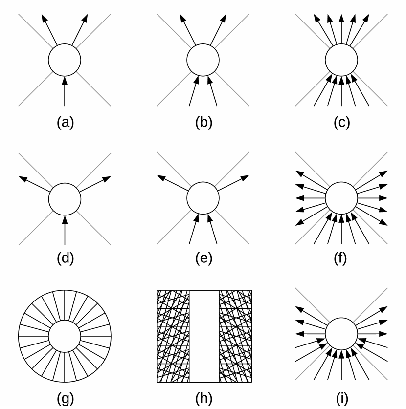
Figure 1: Elementary processes (see description in text).

1 Introduction

Tachyonic models for the description of dark matter have appeared recently. Papers [1, 2, 3] consider a model of tachyonic scalar field, based on the action

$$S[T(x)]=-\int d^{4}x\sqrt{-g}\ V(T)\sqrt{1+\nabla_{\mu}T\nabla^{\mu}T},$$ (1)

where $T(x)$ is a scalar field, $V(T)$ is a given potential function, $\nabla_{\mu}$ is covariant derivative and $d^{4}x\sqrt{-g}$ is invariant integration measure of General Relativity. In this model the distribution of energy-momentum can be decomposed to a sum of pressureless liquid, interpreted as dark matter, and a negative pressure medium, interpreted as dark energy. After fine tuning of the parameters, the model becomes compatible with the standard Big Bang cosmology, providing an explanation for the observed accelerated expansion of the universe.

The paper [4] takes a different approach, considering geodesic flows of particles, described by the action

$$S_{\pm}[x(\tau)]=\mp m\int d\tau\sqrt{\mp\dot{x}_{\mu}\dot{x}^{\mu}},$$ (2)

where $x(\tau)$ is the world line of the particle, $\dot{x}=dx/d\tau$, the upper sign corresponds to normal matter, the lower sign to tachyonic matter and the metric signature $(-,+,+,+)$ is chosen. Considering such flows in non-stationary FRW universe, the paper shows that the curved metric forces the tachyonic world lines to turn back in time, leading to self-annihilation of the tachyons and their disappearance from the universe. We note, however, that a reserve of the tachyons can be renewed, if one admits that the tachyons are created in local singularities, under event horizons, and escape from the black holes along spacelike world lines. In this paper we will consider а tachyonic model in the context [4], as a geodesic flow of particles, and focus our attention on the role that can be played by black holes in this model. Particularly, we study the following scenario.

Let’s consider an isolated spherically symmetric black hole and a flow of particles of normal matter isotropically falling into it from infinity. From a point of view of a distant observer the particles slow down at event horizon and never intersect it, while in a coordinate system moving together with the particles they pass through event horizon and move further towards singularity. The black hole acts like a natural accelerator, where the particles are boosted to extremely high energies. This opens an opportunity for new physics, in particular, we will admit that high energetic collisions of particles lead to generation of tachyons.

Kinematically the processes of transformation of normal matter to tachyons are allowed. The tachyons are superluminal particles possessing opposite sign in mass-shell condition and propagating along spacelike world lines, outside the light cone. Fig.1 shows a collection of various processes happening with normal particles and tachyons. Here time axis is vertical, space axis is horizontal and light cones are shown by grey lines (except of fig.1g, showing purely spatial projection). The vector of energy-momentum of every particle is directed along its world line.

Fig.1a shows a process of decay of one normal particle to two normal particles: $(m,0)\to(m/2,\vec{p})+(m/2,-\vec{p})$ with $(m/2)^{2}-\vec{p}^{\;2}>0$. Fig.1d shows a decay of the same normal particle to two tachyons: $(m/2)^{2}-\vec{p}^{\;2}<0$. In both case the conservation of energy-momentum is satisfied.

Fig.1b shows a collision of two normal particles leading to creation of two other normal particles $(E,\vec{p}_{1})+(E,-\vec{p}_{1})\to(E,\vec{p}_{2})+(E,-\vec{p}_{2})$, with $E^{2}-\vec{p}_{1}^{\;2}>0$ and $E^{2}-\vec{p}_{2}^{\;2}>0$. Fig.1e shows creation of two tachyons, with $E^{2}-\vec{p}_{2}^{\;2}<0$. Here the conservation of energy-momentum is satisfied as well.

Therefore the question here is not in kinematic feasibility but in the existence of interaction vertices allowing these transformations. In this paper we assume that interaction vertices for transformation of normal particles to tachyons exist and are activated at high energies, achievable only under event horizons. At low energies the vertices are suppressed.

A possible mechanism of this suppression can be an existence of a supermassive normal particle to which the tachyons are directly coupled, so that creation of freely propagating tachyons requires an overcoming of a high mass barrier. The other mechanism can be direct dependence of vertex function on the energy. Here we will not fix this mechanism and just assume that under event horizon the normal matter will be converted to tachyons before falling into the singularity.

Since the tachyons are superluminal particles, they are not confined in the black hole and can leave it along spacelike world lines. In this way the falling matter is returned back to our side of the universe in the form of outgoing flow of tachyons. Outside the black hole the tachyons do not interact directly with the normal matter and with each other and move freely along the geodesics. On the other hand, since the tachyonic flows have non-zero density of energy-momentum, they are able to curve the space-time and produce observable gravitational effects. Thus the tachyonic flows outside of event horizons behave like invisible type of matter interacting with the normal matter only gravitationally, making it a suitable candidate for the role of astrophysical dark matter.

In further detail, Fig.1c shows a process of multiple collision of normal particles transformed to a shower of normal particles. Kinematically the outgoing particles can occupy the future light cone of collision point. Fig.1f shows analogous process producing a shower of tachyons, occupying the exterior part of the light cone. Conservation of momentum can be easily fulfilled e.g. by considering spherically symmetrical incoming and outgoing flows. Conservation of energy is recorded as equality of total energy for incoming and outgoing flows. It is a single integral equation leaving enough degrees of freedom for setting detailed distributions of energy in the flows.

For the case of tachyons, there are world lines in the exterior of the light cone going forward in time and there are world lines going backward in time. These types of world lines cannot be separated in Lorentz invariant way, i.e. this separation depends on the choice of a reference frame. The vector of energy-momentum is directed along the world lines, so that world lines going backward in time possess negative energy. They can be also considered as the world lines going forward in time and possessing positive energy, like shown on Fig.1i.

All physically meaningful relativistic models are invariant under reversal of the direction of the world lines, which actually just a convention where the world line starts and where ends. E.g. the action of tachyons is the length of the world line, invariant under its reversal. We will see further that tensor of energy-momentum for tachyonic flow is quadratic in velocities and reversal of the velocities does not change it either. Thus the reversal of the world lines changes only the interpretation, while the flows depicted on Fig.1f and Fig.1i produce physically equivalent answers. In summary, Fig.1i shows incoming flow of normal matter, incoming flow of tachyons and outgoing flow of tachyons, while outgoing flow of normal matter is completely blocked by the black hole. Note that in this interpretation all flows have positive energy.

Further, we will consider not only a single collision event, but a stationary process supported by these flows. I.e. we consider incoming flows of normal matter and tachyons as permanently sourced at infinity and absorbed by the black hole and outgoing flow of tachyons as permanently emitted by the black hole and sinked at infinity. Although such stationarity is not absolutely necessary, it simplifies a lot the computation of gravitational effects. To make the process stationary, we need to superimpose multiple copies of Fig.1i shifted along time axis and form the distribution of world lines shown on Fig.1h.

Also for our convenience, we will consider spherically symmetric distributions and restrict computations to a finite spherical layer $r\in[r_{1},r_{2}]$, schematically shown on spatial projection Fig.1g. In this way all unknown processes become located outside of the considered domain: at $r<r_{1}$ there are processes of transformation of normal matter to tachyons, at $r>r_{2}$ there are processes permanently sourcing incoming flows and sinking outgoing flows. Inside spherical layer there are only geodesic flows of matter and curved space-time, whose known physics allows us to perform straightforward computations.

In Section 2 we consider dynamics of tachyons in comparison with the dynamics of normal particles. In Section 3 we set energy-momentum tensor for the above described spherically symmetric stationary problem. In Section 4 we solve Einstein equations in the limit of weak fields. In Section 5 we discuss the obtained results and outline possible extensions of the model.

2 Dynamics of tachyons

The world lines of the particles are stationary points of the action

$$S_{\pm}[x(\tau)]=\mp m\int d\tau\sqrt{\mp g_{\mu\nu}\dot{x}^{\mu}\dot{x}^{\nu}},$$ (3)

We remind that General Relativity (GR) distinguishes between upper tensor indices (called contravariant) and lower tensor indices (called covariant) and

• $g^{\mu\nu}$ is inverse to $g_{\mu\nu}$,

• metric tensor is used to raise and lower the indices,
  e.g. $x_{\mu}=g_{\mu\nu}x^{\nu}$, $x^{\mu}=g^{\mu\nu}x_{\nu}$,

• summation over repeating indices is everywhere assumed,

• length element in space-time is $ds^{2}=g_{\mu\nu}dx^{\mu}dx^{\nu}$,

• invariant integration measure is $d^{4}x\sqrt{-g}$, where $g=\det g_{\mu\nu}$,

• $\nabla$ denotes covariant derivative, $\Gamma$ are Christoffel symbols:

  $$\Gamma^{\mu}_{\nu\lambda}=\frac{1}{2}g^{\mu\rho}(\partial_{\lambda}g_{\rho\nu}+\partial_{\nu}g_{\rho\lambda}-\partial_{\rho}g_{\nu\lambda})$$

  $$\nabla_{\alpha}V^{\mu}=\partial_{\alpha}V^{\mu}+\Gamma^{\mu}_{\alpha\lambda}V^{\lambda},$$

  $$\nabla_{\alpha}T^{\mu\nu}=\partial_{\alpha}T^{\mu\nu}+\Gamma^{\mu}_{\alpha\lambda}T^{\lambda\nu}+\Gamma^{\nu}_{\alpha\lambda}T^{\mu\lambda},\ \mbox{etc.}$$

The integral (3) defines total length of the world line in curved metric and its extremum corresponds to geodesics. Special relativity (SR) corresponds to flat metric $\eta_{\mu\nu}=\mbox{diag}(-1,1,1,1)$ and straight geodesic lines.

Upper sign in the action corresponds to timelike world lines $ds^{2}<0$, i.e. the particles of normal matter (in the literature also called tardyons or bradyons). Lower sign corresponds to spacelike world lines $ds^{2}>0$, the tachyons. Overall sign is selected in a way that canonical momentum $p_{\mu}=\delta S_{\pm}/\delta\dot{x}^{\mu}$ in contravariant recording

$$p^{\mu}=m\dot{x}^{\mu}/\sqrt{\mp\dot{x}^{\alpha}\dot{x}_{\alpha}}$$ (4)

would have positive temporal component, for the world lines directed in the future and $m>0$. This convention ensures positive energy for the particles. Mass shell condition has a form

$$p^{\mu}p_{\mu}=\mp m^{2},$$ (5)

so that for normal particles $m$ can be identified with the mass of the particle. Tachyons are often described as particles with imaginary mass, but we will consider $m$ as real parameter and for tachyons explicitly fix a different sign in the mass shell condition.

Remark about negative masses: the case of $m<0$ is usually called exotic matter and corresponds indeed to very unusual effects, like repelling gravitational force (anti-gravitation). For tachyons the case $m<0$ would be double exotic, describing spacelike world lines with momentum vector opposite to the direction of the world line. In our model we will use only positive masses. Although negative masses are theoretically possible, they are not needed for a moment.

Remark about causality principle: involving tachyons in the model, one could expect causality violations, since one can make tachyons to propagate back in time simply by a change of coordinate frame. However, we have seen that the reversal of the world line of the tachyon leaves its physics invariant. Also, a possibility to transmit information by tachyons implies an ability to interact with them, while in our model all points of direct interaction are hidden under event horizons. Although the tachyons can interact with the normal matter gravitationally, these effects, as all effects related to the dark matter, are supposedly detectable only on large astronomical scale. We are curious if it will be possible to construct a measurable violation of causality principle under these conditions. In this relation we refer to classical work of Wheeler and Feynman [5, 6] about advanced and retarded interactions, where the questions of causality violation have been analyzed in detail.

3 Setting energy-momentum tensor

Tensor of energy-momentum is defined by the formula

$$T^{\mu\nu}(x)=2(-g)^{-1/2}\;\delta S/\delta g_{\mu\nu}(x)$$

and for a pointlike particle can be written as

$$T^{\mu\nu}=(-g)^{-1/2}\;m\int d\tau\;\delta(x(\tau)-x)\;\dot{x}^{\mu}\dot{x}^{\nu}/\sqrt{\mp\dot{x}^{\alpha}\dot{x}_{\alpha}},$$

or equivalently:

$$T^{\mu\nu}=\rho u^{\mu}u^{\nu},\ \rho=(-g)^{-1/2}\;m\int ds\;\delta(x(s)-x),\ u^{\mu}=(dx^{\mu}(s)/ds)|_{x(s)=x}.$$

Here $ds=(|ds^{2}|)^{1/2}$ introduces natural parametrization on the world line, $u^{\mu}$ is a tangent vector to the world line, with proper normalization:

$$u^{\mu}u_{\mu}=\mp 1,\ u^{\mu}=p^{\mu}/m.$$

The factor $(-g)^{-1/2}$ makes $\rho$ invariant (scalar) under diffemorphisms of $x$ and corresponding transformation of metric. $\rho(-g)^{1/2}d^{4}x$ gives a mass element, $\rho$ represents a density of mass per invariant volume $(-g)^{1/2}d^{4}x$, while $\rho(-g)^{1/2}$ represents a density of mass per standard volume $d^{4}x$. In the considered case the function $\rho(-g)^{1/2}$ is singular, it describes a positive mass localized on the world line, uniformly distributed on it with respect to the natural parameter. The shift of points along the world line $x(s)\to x(s+ds)$ preserves this mass distribution. Foliating the space-time to such world lines, we have a tensor of energy-momentum for the flow of particles in the form:

$$T^{\mu\nu}=\rho u^{\mu}u^{\nu},\ \rho>0,$$ (6)

where $u^{\mu}$ is the velocity of the flow in the given point. The density $\rho(-g)^{1/2}$ is again invariant under the shifts of points along the world lines, i.e. is preserved by the flow, following standard continuity equation $\partial_{\mu}(\rho(-g)^{1/2}u^{\mu})=0$. Using the identity $\partial_{\mu}((-g)^{1/2}V^{\mu})=(-g)^{1/2}\nabla_{\mu}V^{\mu}$ from [7], we can rewrite this equation in covariant form as

$$\ \nabla_{\mu}(\rho u^{\mu})=0.$$ (7)

Note that (6) and (7) are well known formulae for a pressureless liquid or for a dust, we just ensure that their derivation does not rely upon normal or tachyonic type of matter, so they are also valid for tachyonic flows.

Further in this section we will use flat metric, fix spherical coordinates $x=(t,r,\theta,\phi)$ and consider the flows depicted on Fig.1f. The world lines can be parametrized as follows:

$$x^{\mu}_{+}(s;\beta,t_{0},\theta_{0},\phi_{0})=(s\cosh\beta+t_{0},s\sinh\beta,\theta_{0},\phi_{0}),\ \mbox{for normal matter;}$$

$$x^{\mu}_{-}(s;\beta,t_{0},\theta_{0},\phi_{0})=(s\sinh\beta+t_{0},s\cosh\beta,\theta_{0},\phi_{0}),\ \mbox{for tachyons.}$$

The velocities are

$$u^{\mu}_{+}(\beta)=(\cosh\beta,\sinh\beta,0,0),\ \mbox{for normal matter;}$$

$$u^{\mu}_{-}(\beta)=(\sinh\beta,\cosh\beta,0,0),\ \mbox{for tachyons.}$$

The density function satisfying mass conservation (7) has a form $\rho(r)=r^{-2}\rho_{1}$ with a constant $\rho_{1}>0$. Such dependence is clear from geometrical point of view: the density of the world lines increases towards the origin inverse quadratically with the distance. It is also clear physically: considering particles in a shell $[r,r+dr]$ moving at a constant speed towards the origin, the mass density will have the same behavior. The overall flow distribution can be parametrized as follows:

$$T^{\mu\nu}(r)=r^{-2}\int d\beta(\rho_{+}u^{\mu}_{+}u^{\nu}_{+}+\rho_{-}u^{\mu}_{-}u^{\nu}_{-}),$$

where $\rho_{\pm}(\beta)>0$ are arbitrary profile functions. Here $\beta<0$ corresponds to inflow, $\beta>0$ to outflow. Since the flow of normal matter depicted on Fig.1f has no outflow component, one can formally extend $\rho_{\pm}(\beta)\geq 0$ to the whole axis and set $\rho_{+}(\beta)=0$ at $\beta>0$.

We will also require that the flows are energetically balanced, i.e. the energies of incoming and outgoing flows coincide. This is equivalent to vanishing total flow of energy through the spatial 2-spheres, i.e. $T^{tr}=T^{rt}=0$. This is a single integral relation which must be satisfied by profile functions $\rho_{\pm}(\beta)$. The only non-zero components of energy-momentum tensor are therefore:

$$T^{tt}=r^{-2}C_{1},\ T^{rr}=r^{-2}C_{2},$$ (8)

where the constants $C_{1,2}>0$ and

$$C_{1}=\int d\beta(\rho_{+}(\beta)\cosh^{2}\beta+\rho_{-}(\beta)\sinh^{2}\beta),$$

$$C_{2}=\int d\beta(\rho_{+}(\beta)\sinh^{2}\beta+\rho_{-}(\beta)\cosh^{2}\beta),$$ (9)

$$C_{0}=\int d\beta(\rho_{+}(\beta)+\rho_{-}(\beta))\sinh\beta\cosh\beta=0.$$

Note that condition of energetic balance $C_{0}=0$ can be satisfied also when the inflow of normal matter is completely switched off: $\rho_{+}(\beta)=0$. In this case the energetic balance must be satisfied by tachyonic flows: incoming flow of tachyons should have the same total energy as outgoing flow of tachyons. Further we give several examples of flow distributions satisfying all necessary conditions.

Example 1: tachyonic flow with symmetric profile

$$\rho_{+}(\beta)=0,\ \rho_{-}(\beta)=\rho_{-}(-\beta).$$

Example 2: flow of normal matter with symmetric profile

$$\rho_{+}(\beta)=\rho_{+}(-\beta),\ \rho_{-}(\beta)=0.$$

Note that this generally requires a presence of outflow for normal matter. This scenario is only possible if the incoming flow of normal matter turns back before reaching event horizon.

Example 3: normal matter in slow limit

$$\rho_{+}(\beta)=\delta(\beta),\ \rho_{-}(\beta)=0.$$

A marginal scenario, depicted on Fig.2a. The only possible flow configuration without tachyons and without outgoing flow of normal matter. Can be considered as incoming flow in the limit $\beta\to-0$. Note that spatial distribution of matter here is not arbitrary and must satisfy $\rho(r)\sim r^{-2}$. The case corresponds to $C_{1}=1$, $C_{2}=0$.

Example 4: “tachyonic monopole”

$$\rho_{+}(\beta)=0,\ \rho_{-}(\beta)=\delta(\beta).$$

Scenario depicted on Fig.2b. The world lines go in purely spatial direction, orthogonally to time axis. In spatial projection this configuration looks like a point surrounded by radially diverging tachyonic fibers, Fig.2c. This case corresponds to $C_{1}=0$, $C_{2}=1$.

Figure 2: Examples of flow distributions: (a) normal matter in slow limit, (b,c) “tachyonic monopole”.

Figure 3: Region of parameter variation: (a) in space $(D_{1},D_{2},D_{0})$, (b) in cross-section $D_{1}=1$.

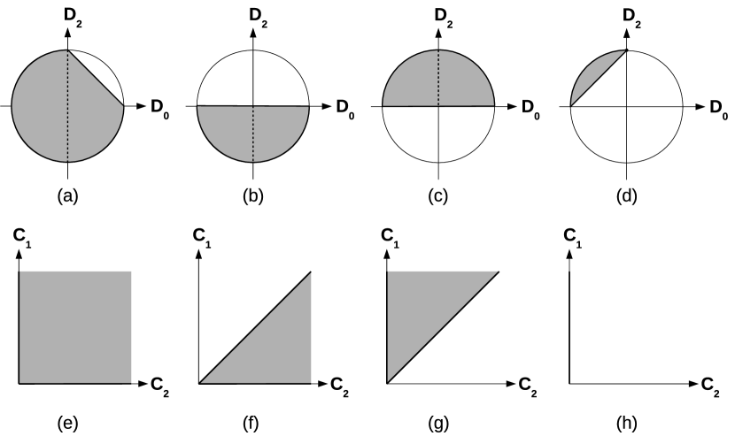
Figure 4: Regions of parameter variation for various scenarios (see description in text).

Further we will clarify which regions on the plane $(C_{1},C_{2})$ can be occupied by different types of flow distributions. Let’s consider (9) as a mapping of non-negative functions $\rho_{\pm}(\beta)$ to 3-dimensional space:

$$(C_{1},C_{2},C_{0})=\int d\beta(\rho_{+}(\beta)\gamma_{+}(\beta)+\rho_{-}(\beta)\gamma_{-}(\beta)),$$

$$\gamma_{+}(\beta)=(\cosh^{2}\beta,\sinh^{2}\beta,\sinh\beta\cosh\beta),$$

$$\gamma_{-}(\beta)=(\sinh^{2}\beta,\cosh^{2}\beta,\sinh\beta\cosh\beta).$$

Performing transformations

$$D_{1}=C_{1}+C_{2},\ D_{2}=C_{1}-C_{2},\ D_{0}=2C_{0},$$

we have

$$(D_{1},D_{2},D_{0})=\int d\beta(\rho_{+}(\beta)\gamma_{+}(\beta)+\rho_{-}(\beta)\gamma_{-}(\beta)),$$

$$\gamma_{\pm}(\beta)=(\cosh 2\beta,\pm 1,\sinh 2\beta).$$ (10)

The curves $\gamma_{\pm}$ form conic sections, shown on Fig.3a. The figure also shows different segments of the curves, corresponding to inflows and outflows: $\gamma_{\pm i,o}$. Vectors $\rho_{\pm}\gamma_{\pm}$ with $\rho_{\pm}>0$ define rays from the origin to the points of the curves. The mapping (10) defines a convex hull of these rays. The result will be different dependently on which parts of the curves are taken in the scenario. The cone has an equation:

$$D_{1}^{2}=D_{2}^{2}+D_{0}^{2}.$$

In cross-section $D_{1}=1$ the problem is reduced to taking convex hulls of corresponding circular arcs, see Fig.3b. Further we need to take a cross-section $D_{0}=0$, representing the equation of energetic balance. Transforming the result in original coordinates, we obtain the regions on a plane $(C_{1},C_{2})$ we are looking for. Several possibilities are considered on Fig.4.

Case 1: Fig.4a,e, inflow of normal matter, inflow and outflow of tachyons

$$C_{1}\geq 0,\ C_{2}\geq 0.$$

Case 2: Fig.4b,f, only tachyons, inflow and outflow

$$C_{2}\geq C_{1}\geq 0.$$

Case 3: Fig.4c,g, only normal matter, inflow and outflow

$$C_{1}\geq C_{2}\geq 0.$$

This scenario is only possible if the incoming flow of normal matter turns back before reaching event horizon.

Case 4: Fig.4d,h, only normal matter, inflow, the marginal case from Example 3

$$C_{1}\geq 0,\ C_{2}=0.$$

The limiting lines on these plots correspond to

• $C_{1}\geq 0,\ C_{2}=0$, slow normal matter

• $C_{2}\geq 0,\ C_{1}=0$, “tachyonic monopole”

• $C_{1}=C_{2}\geq 0$, Cases 2,3, a limit of lightlight particles, $\beta\to\infty$.

4 Solving Einstein field equations

The equations have a form:

$$R_{\mu\nu}-\frac{1}{2}g_{\mu\nu}R=8\pi GT_{\mu\nu},$$ (11)

where $g_{\mu\nu}$ is metric tensor, $R_{\mu\nu}$ is Ricci curvature tensor, $R=g^{\mu\nu}R_{\mu\nu}$, $T_{\mu\nu}$ is energy-momentum tensor, $G$ is gravitational constant. Further we fix a system of units $4\pi G=1$. Ricci tensor is a sophisticated non-linear function of metric tensor and its first and second derivatives, whose explicit expression can be found in [7, 8].

Before proceeding to solution, there are some introductory remarks. At first, not all components of Einstein field equations are independent. There is a compatibility requirement, equivalent to continuity condition on energy-momentum tensor: $\nabla_{\mu}T^{\mu\nu}=0$. For the flows of free falling particles this condition is equivalent to the motion of particles along geodesics. Thus, the system (11) incorporates a condition on matter distribution, the flow must be geodesic.

Secondly, GR is invariant under diffeomorphisms of coordinates and corresponding transformations of metric tensor. A set of general solutions of Einstein field equations contains together with every solution all its diffeomorphisms. To fix this freedom, gauge conditions are selected, equivalent to a choice of particular coordinate system, e.g. synchronous coordinates $g_{0i}=0,\ i>0$.

In this paper we will solve not the general system (11), but its linearization. Namely, we will consider slightly curved metric, represented in the form $g_{\mu\nu}=\eta_{\mu\nu}+h_{\mu\nu}$, where $\eta_{\mu\nu}$ is the flat metric and $h_{\mu\nu}$ is a small correction. Energy-momentum tensor from the previous section corresponds to geodesic flows of particles in flat metric. We substitute this matter contribution to the right hand side of (11), consider it as small correction to vacuum case and solve the system for the linear term $h_{\mu\nu}$. According to approximation schemes [9], this solution can be used further to correct the geodesics and compute higher order terms. In this paper we restrict ourselves to the investigation of linear correction and its influence to the motion of probe particles.

For spherically symmetric stationary problems one can choose the metric in the form [7, 8]:

$$ds^{2}=-A(r)dt^{2}+B(r)dr^{2}+r^{2}(d\theta^{2}+\sin^{2}\theta d\phi^{2}),$$

where after substitution

$$A(r)=e^{2h(r)}f(r),\ B(r)=f(r)^{-1},\ f(r)=1-2m(r)/r$$

the system (11) is reduced to

$$m^{\prime}(r)=r^{2}(-T^{t}_{t}),\ h^{\prime}(r)=rf(r)^{-1}(-T^{t}_{t}+T^{r}_{r}).$$

We substitute here the components of energy-momentum tensor (8) and use flat metric to raise and lower the indices: $T^{t}_{t}=-T^{tt}$, $T^{r}_{r}=T^{rr}$. The difference between real and flat metric being multiplied to small $T$-components becomes a higher order term, which can be neglected in considered approximation. Thus we have

$$m^{\prime}(r)=C_{1},\ h^{\prime}(r)={C_{1}+C_{2}\over r-2m(r)}.$$

Solution has a form:

$$m(r)=C_{1}r+C_{3},\ h(r)=\epsilon\log|r-r_{0}|+C_{4},$$

with two new integration constants $C_{3,4}$ and

$$\epsilon={C_{1}+C_{2}\over 1-2C_{1}},\ r_{0}={2C_{3}\over 1-2C_{1}}.$$

The term $C_{3}$ corresponds to an arbitrary mass, located at the origin or distributed spherically symmetrically under $r<r_{1}$, inside the inner sphere of the considered spherical layer. The constant $C_{4}$ can be absorbed in definition of time and fixed arbitrarily, e.g by requiring $h(r_{1})=0$.

If, for a moment, we set the constants $C_{1,2}$ to zero, these formulae reconstruct well known Schwarzschild’s solution for spherically symmetric black hole, with parameter $r_{0}$ representing Schwarzschild’s radius:

$$r_{0}=2C_{3},\ m(r)=C_{3},\ h(r)=0,$$

$$A(r)=(1-r_{0}/r),\ B(r)=(1-r_{0}/r)^{-1}.$$

Further, considering the case of non-zero $C_{1,2}$, we should keep the solution in the frames of admitted approximation, the metric should deviate only slightly from the flat case. This implies $|A(r)-1|\ll 1$, $|B(r)-1|\ll 1$, or equivalently $|2m(r)/r|\ll 1$, $|h(r)|\ll 1$ everywhere in the considered range $r\in[r_{1},r_{2}]$. This can be achieved by fixing $r_{1}\ll r_{2}$ and selecting sufficiently small constants satisfying $C_{1}\ll 1$, $2C_{3}\ll r_{1}$, $(C_{1}+C_{2})\log r_{2}/r_{1}\ll 1$. The first condition keeps us away from the pole appeared in $r_{0}$-definition, the second one requires that the considered spherical layer is well above Schwarzschild’s radius and the third one ensures that our matter distribution produces small curvature of space-time in between $r_{1}$ and $r_{2}$. Equivalently, one can select $C_{1}\ll 1$, $r_{0}\ll r_{1}$, $\epsilon\ll(\log r_{2}/r_{1})^{-1}$. In this limit we have

$$\epsilon=C_{1}+C_{2},\ r_{0}=2C_{3},\ h(r)=\epsilon\log r/r_{1},\ f(r)=1-2C_{1}-r_{0}/r,$$

$$A(r)=1-2C_{1}+2\epsilon\log r/r_{1}-r_{0}/r,\ B(r)=1+2C_{1}+r_{0}/r.$$

Thus we have for temporal component of metric tensor

$$g_{00}=-A(r)=-1+2C_{1}-2\epsilon\log r/r_{1}+r_{0}/r.$$

This component is related with gravitational potential, describing geodesic motion of non-relativistic probe particles [7, 8]:

$$g_{00}=-1-2\phi,\ \ddot{x}=-\mbox{grad}\;\phi,$$

thus we have

$$\phi=-C_{1}+\epsilon\log r/r_{1}-r_{0}/(2r),$$

the probe particles possess acceleration directed radially towards the origin

$$a_{r}=\epsilon/r+r_{0}/(2r^{2}).$$

Here the second term corresponds to Newton’s law, becoming $GM/r^{2}$ after reconstruction of physical units. The first term is the effect of matter distribution constructed in our model. Considering circular orbits around the origin and substituting $a_{r}=v^{2}/r$, we have for the orbital velocity

$$v^{2}=\epsilon+r_{0}/(2r).$$ (12)

At large $r$ the velocity does not tend to zero, as it should be for purely Newtonian case. Instead, it tends to a positive constant value.

Figure 5: Measured velocities of stars in galaxies, as a function of distance to the center, data from [11].

5 Discussion

Dependence of orbital velocity on radius with asymptotic transition to non-zero constant shows a similarity with the measured rotation curves of the galaxies, see fig.5. In 1978 Vera Rubin and coworkers have shown that the velocities of stars and interstellar gas in high-luminosity spiral galaxies are constant in wide range of distances [10]. The estimation involving only luminous matter provided much smaller velocities and the rotation curves falling with the distance. Attempts to explain this discrepancy gave birth to the concept of hidden mass, also known as dark matter. As we see, tachyonic models are well suited for the role of dark matter. Already our simple model describes important qualitative features as increased orbital velocity and asymptotically constant rotation curve. Of course, this model is still too idealized for comparison with a real galaxy, in fact, from the necessary elements it contains only the central supermassive black hole. To explain fine details of the rotation curves, one should take into account the distribution of luminous matter, the presence of other black holes in the galaxy and the influence of gravitational field to the shape of tachyonic world lines.

One such fine detail can be an observable deviation of rotation curve from the constant. According to [11], this deviation depends on luminosity of the galaxy: most luminous galaxies have slightly decreasing rotation curves, intermediate luminosities correspond to constant rotation curves, low-luminosity galaxies have increasing rotation curves. In particular, low-luminosity dwarf galaxy M33 shows slightly increasing rotation curve [12]. The measurement of 21 spiral galaxies of Sc type shows that most of them have slightly increasing rotation curves [13]. The deviation of rotation curve from the constant can be explained by the presence of the other black holes, i.e. sources and sinks of dark matter distributed over the galaxy, which can lead to the dark matter term $\epsilon(r)$ dependent on the distance to the center of the galaxy. In weak field approximation the sources contribute additively to the gravitational potential and a sum of isotropic sources will give the dark matter term increasing with the distance, providing the increasing rotation curve. On the other hand, if the tachyonic world lines sourced by the central black hole will sink in the other black holes distributed over the galaxy, the distribution of dark matter can be truncated and one can see falling rotation curves outside of truncation radius. These scenarios will require more complex computations, based on non-isotropic flows and non-straight tachyonic world lines.

At a larger scale dark matter forms superstructures, they look like a network of filaments connecting the galaxies [14]. Such spacelike structures can be composed of tachyonic world lines stretched between the galactic black holes. Theoretically, these networks can also connect white holes and other places where conditions are hot enough, Big Bang, Big Crunch, etc. In the models describing multiple universes [15] tachyonic world lines will not be confined in one universe and can pass from one universe to another. Analysis of such scenarios would also require more sophisticated methods and presumably can be done only with the aid of numerical simulations.

The calculations in our paper were done in the limit of weak fields and were similar to those in Newtonian limit. However, the matter distribution involved superluminal particles and Newtonian limit was not applicable as is. The work [9] mentions a combination of different approximations: weak field, near zone, small $v/c$; here we used just the first option. It is interesting to continue the model in the region of strong fields and to look what happens with tachyons under event horizon.

We remind that initial parameters of the model were distributions $\rho_{\pm}(\beta)$. They were contracted to two constants in tensor of energy-momentum, so that the metric actually depends only on two parameters $C_{1,2}$. They were summed in gravitational potential to a single constant $\epsilon$. All these parameters are free, they can be restricted only by inequalities, described in Section 3. The inequalities appear after a priori restrictions on the structure of the flows, e.g. $C_{1}\leq C_{2}$, if the incoming flow of normal matter is completely switched off. On the other hand, the constants can be fixed by a detailed model describing the processes under event horizon (e.g. explaining a proportion between normal and dark components of the flow) and also by external boundary conditions on incoming and outgoing flows (e.g. connecting the flows from different black holes). In this way one can obtain a picture of the universe as a global relativistic network, a cosmic web of tachyonic filaments stretched between the black holes and the galaxies around them. Calculation of equilibrium of such network using analytical and numerical methods would be a challenging problem.

6 Conclusion

We have considered a spherically symmetric stationary problem, including a black hole, incoming and outgoing flows of tachyons and optionally incoming flow of normal matter. Computations in the limit of weak field show that probe particles moving along circular orbits in this model have a dependence of orbital velocity on a distance identical with the typical rotation curves of galaxies. We have discussed a possibility to use the model for a description of dark matter distribution in galaxies and the extensions of the model for a description of more complex scenarios.

References

- [1] G. Shiu, I. Wasserman, Cosmological constraints on tachyon matter, Physics Letters B 541 (2002) 6-15; arXiv:hep-th/0205003.
- [2] A. Frolov, L. Kofman, A. Starobinsky, Prospects and problems of tachyon matter cosmology, Physics Letters B 545 (2002) 8-16; arXiv:hep-th/0204187.
- [3] J.S. Bagla, H.K. Jassal, T. Padmanabhan, Cosmology with tachyon field as dark energy, Phys. Rev. D 67 (2003) 063504; arXiv:astro-ph/0212198.
- [4] P.C.W. Davies, Tachyonic dark matter, Int. J. Theor. Phys. 43 (2004) 141-149; arXiv:astro-ph/0403048.
- [5] J.A. Wheeler, R.P. Feynman, Interaction with the absorber as the mechanism of radiation, Rev. Mod. Phys. 17 (1945) 157-181.
- [6] J.A. Wheeler, R.P. Feynman, Classical electrodynamics in terms of direct interparticle action, Rev. Mod. Phys. 21 (1949) 425-433.
- [7] P.A.M. Dirac, General Theory of Relativity, Princeton University Press, 1996.
- [8] M. Blau, Lecture Notes on General Relativity, Albert Einstein Center for Fundamental Physics, Institute for Theoretical Physics, University of Bern, 2015, http://www.blau.itp.unibe.ch/Lecturenotes.html
- [9] T. Damour, The general relativistic two body problem, in: Frontiers in Relativistic Celestial Mechanics, S.M. Kopeikin (Ed.), Volume 1: Theory, de Gruyter Studies in Mathematical Physics, 2014.
- [10] V.C. Rubin, W.K. Ford, Jr., N. Thonnard, Extended rotation curves of high-luminosity spiral galaxies, The Astrophysical Journal 225 (1978) 107-111.
- [11] Y. Sofue, V.C. Rubin, Rotation curves of spiral galaxies, Ann. Rev. Astron. Astrophys. 39 (2001) 137-174; arXiv:astro-ph/0010594.
- [12] E. Corbelli, P. Salucci, The extended rotation curve and the dark matter halo of M33, Monthly Notices of the Royal Astronomical Society 311 (2000), 441-447; arXiv:astro-ph/9909252.
- [13] V.C. Rubin, W.K. Ford, Jr., N. Thonnard, Rotational properties of 21 Sc galaxies with a large range of luminosities and radii from NGC 4605 (R = 4kpc) to UGC 2885 (R = 122kpc), The Astrophysical Journal 238 (1980) 471-487.
- [14] S. Bharadwaj, S. Bhavsar, J.V. Sheth, The size of the longest filaments in the universe, Astrophys. J. 606 (2004), 25-31; arXiv:astro-ph/0311342.
- [15] M. Tegmark, Parallel Universes, in: Science and Ultimate Reality: from Quantum to Cosmos, honoring John Wheeler’s 90th birthday, Cambridge University Press (2003) 40-51; arXiv:astro-ph/0302131.