Equation of motion of the triple contact line along an inhomogeneous surface

Abstract

The wetting flows are controlled by the contact line motion. We derive an equation that describes the slow time evolution of the triple solid-liquid-fluid contact line for an arbitrary distribution of defects on a solid surface. The capillary rise along a partially wetted infinite vertical wall is considered. The contact line is assumed to be only slightly deformed by the defects. The derived equation is solved exactly for a simple example of a single defect.

1 Introduction

The wetting flows (where the triple solid-liquid-fluid contact line is present) are important for many practical applications ranging from the metal coating to the medical treatment of the lung airways. The contact line statics and dynamics attracted a lot of attention from the scientific community during the last decades. It became clear that the hydrodynamics in the region of the liquid wedge close to the contact line (which we will call CLR - Contact Line Region) differs from the hydrodynamics in the bulk of the liquid. Because of the contact line singularity [1], the fluid motion in presence of the contact line appears to be much slower than without it. This difference can be accounted for by the introduction of the anomalously large energy dissipation inside the CLR [1].

For practical purposes, one needs to know the dynamics of the liquid surface influenced by this dissipation. This influence is especially strong in the very common case of (i) low viscosity fluids that (ii) wet partially the solid with (iii) no precursor film on it. In this case the bulk dissipation is particularly small with respect to the large CLR dissipation [2]. The contact line motion is very slow and the liquid surface can be described in the quasi-static approximation [3]. The dissipation in the liquid (energy per unit time) can then be approximated by the dissipation in the CLR as [4]

$$\int{\xi\,v_{n}^{2}\over 2}\;{\rm d}l,$$ (1)

where $v_{n}$ is the normal component of the contact line velocity and the integration is performed along the contact line. The generalized dissipation coefficient $\xi$ is a constant that is assumed to be much larger that the liquid shear viscosity. The expression (1) assumes that the contribution of a piece of the CLR to the dissipation is proportional to the contact line length. Then the $v_{n}^{2}$ term is leading for small $v_{n}$. The dissipation coefficient $\xi$ can be obtained e.g. from measurements of the kinetics of relaxation of an oval sessile drop toward its equilibrium shape (see [2], where it was found $10^{7}$ times larger than the shear viscosity). It can also be obtained from the measurements of $v_{n}$ and the dynamic contact angle $\theta$ by using the expression

$$v_{n}={\sigma\over\xi}\,(\cos\theta_{eq}-\cos\theta),$$ (2)

where $\theta_{eq}$ is the equilibrium value of the contact angle and $\sigma$ is the surface tension. Eq. 2 is common for many contact line motion models. It can be shown [4] that Eq. 2 follows from the expression (1) for the cases where $v_{n}$ does not vary along the contact line (i.e. for the contact line of constant curvature).

Usually, one is interested to know the displacement of the contact line (or its statistical properties in the case of the irregular solid) because its position serves as a boundary condition for the determination of the shape of the liquid surface. The recent articles on this subject show that no general approach to this problem is accepted. It is recognized generally [5, 6, 7] that the static contact line equation should be non-local because the contact line displacement at one point influences its position at other points through the surface tension. In dynamics, the local relations similar to Eq. 2 were considered universal for a long time. In our previous work [8] we developed a non-local dynamic approach. We showed that if non-locality is taken into account, Eq. 2 is not valid in the general case where $v_{n}$ varies along the contact line. This variation can be due either to the initially inhomogeneous contact line curvature (like in [8]) or to a inhomogeneous substrate. In this Letter we analyze this latter case. We use this non-local approach to derive an equation of motion for the very common case of the capillary rise of the liquid along a vertical solid wall with the account of the surface defects.

2 Derivation of the equation

A Cartesian reference system $xyz$ is chosen in such a way that the liquid surface far from the wall (defined by the $y-z$ plane) coincides with the $x-y$ plane, see Fig. 1. The liquid surface described by the equation $z=f(x,y)$ is assumed to be weakly deformed so that

$$|\partial f/\partial x|,|\partial f/\partial y|\ll 1.$$ (3)

The contact line can be described by the equation $z=h(y)\equiv f(0,y)$. A piece of the liquid surface of length $2L$ in the $y$-direction (see Fig. 1) is considered so that the final form for the equation of motion is found in the limit $L\rightarrow\infty$.

Figure 1: Reference system to describe the shape of the liquid surface.

First, following the approach [5], we find the energy $U$ of the liquid (per contact line length) as a functional of $h$. It is convenient to break $U$ into two terms, $U=U_{1}+U_{2}$. In the approximation (3), the first term reads

$$U_{1}={\sigma\over 4L}\int_{-L}^{L}\textrm{d}y\int_{0}^{\infty}\textrm{d}x\left[\left({\partial f\over\partial x}\right)^{2}+\left({\partial f\over\partial y}\right)^{2}+{f^{2}\over l_{c}^{2}}\right],$$ (4)

where $l_{c}=[\sigma/(\rho g)]^{1/2}$ is the capillary length, $\rho$ is the liquid density and $g$ is the gravity acceleration. The defects are accounted for in the second term [5, 9]

$$U_{2}=-{\sigma\over 2L}\int_{-L}^{L}\textrm{d}y\int_{0}^{h(y)}c(y,z)\,\textrm{d}z$$ (5)

by the fluctuations of the function $c(y,z)$ which is the difference of the surface energies (in $\sigma$ units) of the gas-solid and liquid-solid interfaces at the point $(y,z)$ of the solid surface. According to the Young expression, $c(y,z)=\cos[\theta_{eq}(y,z)]$, where $\theta_{eq}$ is the local value of the equilibrium contact angle. When the surface defects exist, $\theta_{eq}$ is an arbitrary function of $y,z$.

In the quasi-equilibrium approximation, the surface shape $f$ is found by minimization of the functional $U$ resulting in the equation

$$(\partial^{2}f/\partial x^{2})+(\partial^{2}f/\partial y^{2})=f/l_{c}^{2},$$ (6)

which can be solved by separating the variables by using the boundary condition $f(x\rightarrow\infty)=0$ and assuming that the function $f(x,y)$ is bounded at $y\rightarrow\pm\infty$. The solution reads

$$f=h_{0}\exp(-x/l_{c})+\sum_{n=1}^{\infty}[a_{n}\cos(\pi ny/L)+b_{n}\sin(\pi ny/L)]\exp\left(-x\sqrt{l_{c}^{-2}+\pi^{2}n^{2}/L^{2}}\right),$$ (7)

where the coefficients $h_{0}$, $a_{n}$, $b_{n}$ are the coefficients for the Fourier series

$$h(y)=f(x=0)=h_{0}+\sum_{n=1}^{\infty}[a_{n}\cos(\pi ny/L)+b_{n}\sin(\pi ny/L)].$$

They can thus be related to $h(y)$ by the expressions

$$a_{n}={1\over L}\int_{-L}^{L}h(y)\cos{\pi ny\over L}\,\textrm{d}y,\quad b_{n}={1\over L}\int_{-L}^{L}h(y)\sin{\pi ny\over L}\,\textrm{d}y,\quad h_{0}={1\over 2L}\int_{-L}^{L}h(y)\,\textrm{d}y.$$ (8)

One can notice that $h_{0}$ is simply the horizontally averaged displacement of the contact line. The back substitution of Eq. (7) with $h_{0}$, $a_{n}$, $b_{n}$ replaced by their values (8) into Eq. (4) results in the functional

$$U_{1}={\sigma\over 4L^{2}}\int_{-L}^{L}\textrm{d}y\int_{-L}^{L}\textrm{d}y^{\prime}h(y)h(y^{\prime})\Biggl{[}(2l_{c})^{-1}+\sum_{n=1}^{\infty}\cos{\pi n(y-y^{\prime})\over L}\sqrt{{1\over l_{c}^{2}}+{\pi^{2}n^{2}\over L^{2}}}\;\Biggr{]}.$$ (9)

Eq. (5) together with Eq. (9) define the functional $U[h(y)]$.

Now, one needs to calculate the dissipation function $T$ (per unit length). In the approximation (3), $v_{n}^{2}{\rm d}l\approx\dot{h}^{2}{\rm d}y$ in Eq. (1) and

$$T={1\over 2L}\int_{-L}^{L}{\xi\,\dot{h}^{2}\over 2}\;{\rm d}y,$$ (10)

where the dot means a time derivative. The equation of motion can be written in the quasi-static approximation as

$${\delta U[h]\over\delta h}=-{\delta T[\dot{h}]\over\delta\dot{h}},$$ (11)

where $\delta\ldots\over\delta\ldots$ means variational derivative. By substituting Eqs. (5,9,10) into Eq. (11) and taking the variational derivatives, one obtains the dynamic equation of the contact line motion:

$$\dot{h}(y)=-{\sigma\over\xi}\Biggl{[}h_{0}/l_{c}-c(y,h)+{1\over L}\sum_{n=1}^{\infty}\int_{-L}^{L}\textrm{d}y^{\prime}h(y^{\prime})\cos{\pi n(y-y^{\prime})\over L}\sqrt{l_{c}^{-2}+{\pi^{2}n^{2}\over L^{2}}}\Biggr{]},$$ (12)

where $h$ and $h_{0}$ are assumed to be time dependent. The final form for the integral equation for the contact line motion can be obtained by taking the limit $L\rightarrow\infty$:

$$\dot{h}(y)={\sigma\over\xi}\biggl{\{}c(y,h(y))-{1\over\pi}\int_{0}^{\infty}\textrm{d}p\int_{-\infty}^{\infty}\textrm{d}y^{\prime}h(y^{\prime})\cos[p(y-y^{\prime})]\sqrt{l_{c}^{-2}+p^{2}}\biggr{\}}.$$ (13)

To treat the contact line equation, it is convenient to introduce the spatial fluctuation $h_{1}=h-h_{0}$ and solve the equations for $h_{1}$ and $h_{0}$ separately. First, we derive the dynamic equation for $h_{0}$ by integrating Eq. (12) over $y$ from $-L$ to $L$, changing the integration order and dividing by $2L$. The integrals of all terms in the sum are zero and one obtains the following equation for $h_{0}$

$$\dot{h}_{0}=-{\sigma\over\xi}(h_{0}/l_{c}-c_{0}),\quad c_{0}={1\over 2L}\int_{-L}^{L}c(y,h_{1}+h_{0})\,\textrm{d}y,$$ (14)

where $c_{0}$ is the (time dependent) horizontal average of $c$. By subtracting Eq. (14) from Eq. (13) one obtains the equation for $h_{1}$ which has the same form as Eq. (13) where $c$ should be replaced by its fluctuation $c_{1}=c(y,h_{1}+h_{0})-c_{0}$. Equation for $h_{1}$ simplifies in the Fourier space. By making use of the convolution theorem [11], one obtains

$$\dot{\tilde{h}}_{1}={\sigma\over\xi}\left(\tilde{c}_{1}-\tilde{h}_{1}\sqrt{l_{c}^{-2}+k^{2}}\right),$$ (15)

where the tilde over a variable denotes its Fourier transform with the parameter $k$, e.g.

$$\tilde{h}_{1}=\tilde{h}_{1}(k,t)=\int_{-\infty}^{\infty}h_{1}(y,t)\exp(-iky)\,\textrm{d}y.$$ (16)

This concludes the derivation of the equation of contact line motion. The stationary version of Eq. (15) was derived first by Pomeau and Vannimenus [5].

The static contact line position is defined by the minimum of the energy $U[h(y)]$. However, it can exhibit multiple minima that correspond to the metastable states. In this case one needs to choose between them [9] to determine correctly the contact line position and corresponding local contact angle (which are both different in advancing and receding cases). In dynamics, Eq. (13) provides us with an unique solution because the system “knows” the direction of the contact line motion and its history.

3 Simple example

To show the relevance of this approach, we solve rigorously the contact line dynamics for a simple case of a single stripe-shaped defect at the wall,

$$c(y,z)=\left\{\begin{array}[]{cc}c_{d},&|y|\leq\Delta,\\ c_{s},&|y|>\Delta,\end{array}\right.$$ (17)

where $c_{d},c_{s}\leq 1$ and $\Delta$ are constants. Consider first the contact line displacement at equilibrium described by the equations

$$h_{0}^{eq}=c_{0}l_{c},\quad\tilde{h}_{1}^{eq}=\tilde{c}_{1}/\sqrt{l_{c}^{-2}+k^{2}}.$$ (18)

Notice that $c_{0}$ should be small enough so that $f$ defined by Eq. (7) satisfies conditions (3). Obviously, Eq. (14) results in $c_{0}=c_{s}$ and

$$\tilde{h}_{1}^{eq}={2\delta c\sin k\Delta\over k\sqrt{l_{c}^{-2}+k^{2}}},$$ (19)

where $\delta c=c_{d}-c_{s}$.

To show how this result relates to earlier approaches to the single-defect problem, we analyze first the limit $\Delta\rightarrow 0$. The inverse transform can easily be taken using the tables [12] and results in

$$h_{1}^{eq}(y)={2\delta c\Delta\over\pi}K_{0}(y/l_{c}),$$ (20)

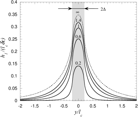
Figure 2: Time evolution of the deviation $h_{1}(y)$ of the contact line from its horizontally averaged value. The defect area (half-width of which is $\Delta=0.2l_{c}$) is shadowed. The time values in the units $\xi l_{c}/\sigma$ are shown above the corresponding curve.

where $K_{0}(\cdot)$ is the modified Bessel function of zeroth order. One recognizes the result [10]. It leads to an unphysical divergence when $y\rightarrow 0$: $h_{1}^{eq}\sim-\log(y)$ and a cut-off at small $y$ is needed [1].

Using the present approach, one can understand the origin of this divergence. The limit $\Delta\rightarrow 0$ in the rigorous result (19) is equivalent to the limit $k\rightarrow 0$ since their product enters Eq. (19). The asymptotics at $k\rightarrow 0$ in the Fourier transform corresponds [11] to the limit $y\rightarrow\infty$ in the original function, which means that Eq. (20) is correct only at $y\rightarrow\infty$. However, it is not guaranteed that its asymptotics at $y\rightarrow 0$ is correct.

Let us return now to the rigorous expression (19). The Fourier transform (19) can be inverted analytically,

$$h_{1}^{eq}(y)=\delta c[F(\Delta+y)+F(\Delta-y)]/\pi,$$ (21)

where $F(y)=\int_{0}^{y}K_{0}(y/l_{c}\,)\,\textrm{d}y$. It is clear now that $h_{1}^{eq}(y\rightarrow 0)$ remains finite, see the dotted curve in Fig. 2.

The dynamic solution can be obtained the same way by using the initial condition $h(t=0)=0$:

$$\begin{array}[]{r}\displaystyle h_{0}(t)=c_{s}l_{c}\{1-\exp[-t\sigma/(\xi l_{c})]\},\\ h_{1}(y,t)=\delta c\left[F(\Delta+y)+F(\Delta-y)\right.\left.-G(\Delta+y,t)-G(\Delta-y,t)\right]/\pi,\end{array}$$ (22)

where

$$G(y,t)=\int_{0}^{y}K_{0}\left(\sqrt{l_{c}^{-2}(y^{2}+t^{2}\sigma^{2}\xi^{-2})}\,\right)\textrm{d}y.$$

The time evolution of $h_{1}(y)$ is shown in Fig. 2. These curves can be compared to those obtained experimentally in [13, 14, 15] where the motion of the contact line over a single defect was studied. The comparison shows a good qualitative agreement. The results cannot be compared quantitatively since in each of these articles some parameters that enter Eq. 22 ($\delta c$ in particular) are missing.

4 Conclusion

Eq. (13) describes the spontaneous contact line motion for arbitrary distribution of surface energy given by the function $c(y,z)$ (provided $|c|$ is small enough so that the conditions (3) are satisfied). This function can be considered random and the equation becomes stochastic. It can be used to establish any statistical parameter of the contact line in dynamics. In particular, the collective effect of defects on the contact line motion can be studied.

In this work we solve a simple example where the defect properties do not vary along the average contact line velocity vector. In the general case, where the local value of the equilibrium contact angle (or of the function $c$) varies along this direction, the equation of the contact line motion becomes non-linear. More sophisticated methods are then needed to solve it.

- [1] P.-G. de Gennes, Rev. Mod. Phys. 57, 827 (1985).
- [2] C. Andrieu, D. A. Beysens, V. S. Nikolayev, & Y.Pomeau, J. Fluid Mech. 453, 427 (2002).
- [3] Y. Pomeau, Comptes Rendus Acad. Sci., Série IIb 328, 411 (2000).
- [4] M.J. de Ruijter, J. De Coninck, and G. Oshanin, Langmuir 15, 2209 (1999).
- [5] Y. Pomeau & J. Vannimenus, J. Colloid Interface Sci. 104, 477 (1984).
- [6] A. Hazareesing & M. Mézard , Phys. Rev. E 60, 1269 (1999).
- [7] J. Vannimenus, Physica A 314, 264 (2002).
- [8] V. S. Nikolayev, & D. A. Beysens, Phys. Rev. E 65, 046135 (2002).
- [9] L. W. Schwartz and S. Garoff, Langmuir 1, 219 (1985).
- [10] J.F. Joanny & M. O. Robbins, J. Chem. Phys. 92, 3206 (1990).
- [11] G. Korn & T. Korn, Mathematical handbook for scientists and engineers, Dover, New York (2000).
- [12] H. Bateman & A. Erdélyi, Tables of Integral transforms, v.1, McGrow-Hill, New York (1954).
- [13] G. D. Nadkarni & S. Garoff, Europhys. Lett. 20, 523 (1992).
- [14] J. M. Marsh & A.-M. Cazabat, Phys. Rev. Lett. 71, 2433 (1993); Europhys. Lett. 23, 45 (1993).
- [15] A. Paterson, M. Fermigier, P. Jenffer, & L. Limat, Phys. Rev. E 51, 1291 (1995).