Emergent behavior in active colloids

Abstract

Active colloids are microscopic particles, which self-propel through viscous fluids by converting energy extracted from their environment into directed motion. We first explain how articial microswimmers move forward by generating near-surface flow fields via self-phoresis or the self-induced Marangoni effect. We then discuss generic features of the dynamics of single active colloids in bulk and in confinement, as well as in the presence of gravity, field gradients, and fluid flow. In the third part, we review the emergent collective behavior of active colloidal suspensions focussing on their structural and dynamic properties. After summarizing experimental observations, we give an overview on the progress in modeling collectively moving active colloids. While active Brownian particles are heavily used to study collective dynamics on large scales, more advanced methods are necessary to explore the importance of hydrodynamic and phoretic particle interactions. Finally, the relevant physical approaches to quantify the emergent collective behavior are presented.

Keywords: active colloids, collective motion, emergent behavior

1 Introduction

Active particles are self-driven units, which are able to move autonomously, i.e., in the absence of external forces and torques, by converting energy into directed motion [1, 2, 3]. In nature many living organisms are active, ranging from mammals at the macro-scale to bacteria at the micro-scale.

Inspired by nature, chemists, physicists, and engineers have started to create and study the motion of artificial nano- and microswimmers [4, 5]. The first experimental realizations, constructed only about ten years ago [6, 7], were actively moving and spinning bimetallic nanorods, driven by a catalytic reaction on one of the two metal surfaces. Since then, many different experimental realizations of nano- and micromachines have been investigated. In particular, spherical active colloids, due to their simple shape, are useful to study novel physical phenomena, which one expects from the intrinsic nonequilibrium nature of autonomous swimmers. Indeed, in experiments they reveal interesting emergent collective properties [8, 9, 10, 11, 12, 13].

The locomotion of microswimmers is governed by low Reynolds number hydrodynamics and thermal noise. Biological microswimmers have to perform periodic, non-reciprocal body deformations or wave long thin appendages in order to swim [14]. In contrast, active colloids and emulsion droplets are able to propel themselves through a viscous medium by creating fluid flow close to their surfaces via self-phoresis or the self-induced Marangoni effect. Hence, their swimming direction is not determined by external forces, such as in driven nonequilibrium systems, but is an intrinsic property of the individual swimmers. Simple models of active colloids are active Brownian particles, which move with a constant speed $v_{0}$ along an intrinsic direction $\mathbf{e}(t)$, which varies in time, e.g., due to rotational Brownian motion. More detailed models for self-phoretic active colloids are not only able to evaluate $v_{0}$ from the local fluid-colloid interaction based on low Reynolds number hydrodynamics, but also determine the surrounding fluid flow and chemical concentration fields. The cooperative motion of self-propelled active colloids, which interact via hydrodynamic, phoretic, electrostatic, and other forces, results in various emergent collective behavior, which we discuss in this Topical Review.

Several reviews on self-propelled particles, microswimmers, and active colloids already exist, many of them with different foci. A general introduction to collective motion can be found in Ref. [1]. The dynamics of active Brownian particles under various conditions is extensively reviewed in Refs. [2] and [3]. Several reviews on the basic fluid mechanical principles of swimming at low Reynolds number are available [15, 16, 17, 18, 19, 20]. How interfacial forces drive phoretic motion of particles is discussed and reviewed in Refs. [21, 22, 4, 5]. More general survey articles about the physics of active colloidal systems are found in [23, 5]. Articles on the fabrication of active colloids, the involved chemical processes, or their control and technical applications exist [24, 25, 26, 27, 28, 29, 30, 31, 32, 33, 34]. Nonequilibrium and thermodynamic properties, as well as motility-induced phase separation and active clustering are discussed in Refs. [35, 36, 37, 38]. We also mention reviews on continuum modeling of microswimmers [39, 40] or of generic active fluids including flocks and active gels [41, 42].

Here we review the emergent behavior in active colloidal systems by focussing on the basic physical concepts. In section 2 we explain how active colloids are able to move autonomously through a fluid. We explain how the basic fluid mechanics at low Reynolds number works (section 2.1), how near-surface flows (section 2.2) or the presence of surfaces (section 2.3) initiate self-propulsion, and introduce the concept of active Brownian particles (section 2.4). In section 3 we discuss generic features of active particles. We present the motion of a single particle in the presence of noise (section 3.1), gravity (section 3.2), taxis (section 3.3), external fluid flow (section 3.4), near surfaces (section 3.5), and in complex environments (section 3.6). The collective dynamics of many interacting active colloids is discussed in section 4. We first review experimental observations in section 4.1, and then address the progress in modeling systems of interacting active colloids in section 4.2. General physical concepts for quantifying emergent collective behavior of active particle suspensions are presented in section 4.3. Finally, we give an outlook in section 5.

2 How do active colloids swim

Passive microscopic particles, such as colloids immersed in a fluid, move when external forces are applied. These can either be external body forces, for example, due to gravity, or surface forces induced by physical or chemical gradients, which then initiate phoretic particle transport [21]. For example, the directed motion of colloids along temperature gradients $\nabla T$, chemical gradients $\nabla c$, or electric potential gradients $\nabla\zeta$, is named thermophoresis, diffusiophoresis, and electrophoresis, respectively [21]. The velocity of the colloids can be calculated using low Reynolds number hydrodynamics.

Active colloids are able to move in a fluid in the absence of external forces. Typically, they create field gradients by themselves localized around their body when they consume fuel [6, 43] or are heated by laser light [44, 45]. This initiates self-phoretic motion [46, 47]. While passive particles move along an externally set field gradient, active colloids change the direction of the self-generated gradient and thereby their propulsion direction, when they experience, for example, rotational thermal noise [43, 48, 44, 45].

Active emulsion droplets start to move when gradients in surface tension form at the fluid-fluid interface by spontaneous symmetry breaking [49, 50, 51, 52]. They then drive Marangoni flow and thereby propel the droplet [53, 54, 55, 8, 56].

In the following we present some basic physical principles of low Reynolds number flow and how active colloids are able to move in Newtonian fluids.

2.1 Hydrodynamics at low Reynolds number: Stokes equations and fundamental solutions

The motion of particles immersed in an incompressible Newtonian fluid with viscosity $\eta$ and density $\rho$ is governed by the Navier Stokes equations [57]. At the micron scale inertial effects can be neglected and the Navier Stokes equations for the flow field $\mathbf{v}(\mathbf{r},t)$ and pressure field $p(\mathbf{r},t)$ simplify to the Stokes equations [58],

$$-\boldsymbol{\nabla}p+\eta\nabla^{2}\mathbf{v}=-\mathbf{f}\enspace,\quad\boldsymbol{\nabla}\cdot\mathbf{v}=0,$$ (1)

where $\mathbf{f}(\mathbf{r},t)$ are body forces acting on the fluid. Together with appropriate boundary conditions at the surface of the particle, equations (1) are solved for $\mathbf{v}(\mathbf{r},t)$ and $p(\mathbf{r},t)$, and one can immediately determine the stress tensor [57]

$$\boldsymbol{\upsigma}=-p\textbf{1}+\eta[\boldsymbol{\nabla}\otimes\mathbf{u}+(\boldsymbol{\nabla}\otimes\mathbf{u})^{t}].$$ (2)

The hydrodynamic force $\mathbf{F}(t)$ and torque $\mathbf{M}(t)$ acting on a body immersed in a Newtonian fluid are then calculated by integrating the stress tensor along the body surface $S$,

$$\mathbf{F}(t) =\int_{S}\boldsymbol{\upsigma}(\mathbf{r},t)\mathbf{n}\,\mathrm{d}S,$$ (3)

$$\mathbf{M}(t) =\int_{S}\mathbf{r}\times(\boldsymbol{\upsigma}(\mathbf{r},t)\mathbf{n})\,\mathrm{d}S.$$ (4)

Here, $\mathbf{n}$ is a unit vector normal to the surface and pointing into the body.

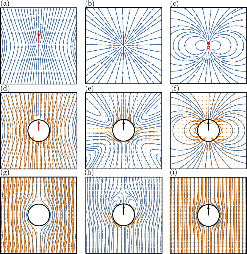
Figure 1: Typical velocity fields (orange) and stream lines (blue) of colloidal objects that behave like a stokeslet (a,d,g), a force dipole (b,e,h), and a source dipole (c,f,i) in the far field. The first line shows the pure flow singularities. The second line shows the flow fields around spherical particles: (d) driven by an external force, (e) a pusher squirmer with $\beta=-3$, and (f) a neutral squirmer with $\beta=0$. The third line shows the flow fields in the frame of the moving particles. The red vectors indicate forces and the black vectors swimming velocities. The source dipole is indicated by a filled circle (source) and an open circle (sink). Two-dimensional slices of the three-dimensional flow fields are shown.

Equations (1) are linear in $\mathbf{v}(\mathbf{r},t)$ and $p(\mathbf{r},t)$ and it is possible to solve for both fields using Green’s functions acting on the inhomogeneity $\mathbf{f}(\mathbf{r},t)$ in the Stokes equations. The unique solution is formally written as [59]

$$\mathbf{v}(\mathbf{r},t) =\int\textbf{{O}}(\mathbf{r}-\mathbf{r}^{\prime})\,\mathbf{f}(\mathbf{r}^{\prime},t)\,\mathrm{d}^{3}x^{\prime},$$ (5)

$$p(\mathbf{r},t) =\int\mathbf{g}(\mathbf{r}-\mathbf{r}^{\prime})\cdot\mathbf{f}(\mathbf{r}^{\prime},t)\,\mathrm{d}^{3}x^{\prime},$$ (6)

where $\textbf{{O}}(\mathbf{r}-\mathbf{r}^{\prime})$ and $\mathbf{g}(\mathbf{r}-\mathbf{r}^{\prime})$ are called Oseen tensor and pressure vector, respectively. In three dimensions they read [59],

$$\textbf{{O}}(\mathbf{r}) =\frac{1}{8\pi\eta}\left(\frac{1}{|\mathbf{r}|}\mathbf{1}+\frac{\mathbf{r}\otimes\mathbf{r}}{|\mathbf{r}|^{3}}\right),$$ (7)

$$\mathbf{g}(\mathbf{r}) =\frac{1}{4\pi}\frac{\mathbf{r}}{|\mathbf{r}|^{3}}.$$ (8)

Now, consider a static point force or force monopole $\mathbf{f}=f\mathbf{e}\delta(\mathbf{r}-\mathbf{r}_{0})$ located at position $\mathbf{r}_{0}$ with strength $f$ and directed along $\mathbf{e}$ in an unbounded fluid, where $\delta(\cdots)$ is the Dirac $\delta$-function. Using equation (5) the resulting flow field, a stokeslet, then simply is

$$\mathbf{v}_{S}(\mathbf{r})=\frac{f}{8\pi\eta r}[\mathbf{e}+(\hat{\mathbf{r}}\cdot\mathbf{e})\hat{\mathbf{r}}].$$ (9)

It decays as $r^{-1}$ with $r=|\mathbf{r}-\mathbf{r}_{0}|$ and $\hat{\mathbf{r}}=(\mathbf{r}-\mathbf{r}_{0})/r$ is the radial unit vector. The streamlines around a stokeslet are illustrated in figure 1(a). The stokeslet is the fundamental solution of the Stokes equations. It describes the flow field far away from the particle, when it is forced from outside, for example, by gravity. Similar as in electrostatics, one can construct solutions of the Stokes equations of higher order in $1/r$ by a multipole expansion of the flow field. The contributions are called force dipole $\sim r^{-2}$, force quadrupole $\sim r^{-3}$, and so on [60, 61, 62, 63]. The force dipole consists of two point forces, $\mathbf{f}=f\mathbf{e}\delta(\mathbf{r}-\mathbf{r}_{0}-(l/2)\mathbf{e})$ and $-\mathbf{f}=-f\mathbf{e}\delta(\mathbf{r}-\mathbf{r}_{0}+(l/2)\mathbf{e})$, separated by a distance $l$. At $r\gg l$ or in the limit $l\rightarrow 0$ the force dipole flow field reads

$$\mathbf{v}_{D}(\mathbf{r})=\frac{p}{8\pi\eta r^{2}}\left[-1+3(\mathbf{e}\cdot\hat{\mathbf{r}})^{2}\right]\hat{\mathbf{r}},$$ (10)

where $p=fl$ is the strength of the force dipole. For $p\propto f>0$, we plot the flow field in figure 1(b). Since the two point forces point outwards, the flow field is called extensile. In contrast, two point forces pointing towards each other ($p<0$) initiate a contractile flow field and the field lines of figure 1(b) are simply reversed. The flow fields of microswimmers are often dominated by force dipoles. Microswimmers with extensile flow fields ($p>0$) are called pushers, since they push fluid outwards along their body axis. Those with contractile flow fields ($p<0$) are called pullers, since they pull fluid inwards along their body axis [15].

In addition to force singularities also source singularities exist. Since they solve the Stokes equations for constant pressure, which gives the Laplace equation, they are potential flow solutions. Combinations of sources and sinks in the fluid are named source monopole $\sim r^{-2}$, source dipole $\sim r^{-3}$, source quadrupole $\sim r^{-4}$, and so on. In figure 1(c) we show the source-dipole flow field,

$$\mathbf{v}_{SD}(\mathbf{r})=\frac{q}{8\pi\eta r^{3}}\left[-\mathbf{e}+3(\mathbf{e}\cdot\hat{\mathbf{r}})\hat{\mathbf{r}}\right],$$ (11)

where $q$ is the source-dipole strength. Higher-order solutions can be constructed by combining lower multipoles. A general flow field solving the Stokes equations can be expressed as a sum of all relevant force and source singularities [60, 61, 62, 63].

The flow singularities describe the far field of colloids moving in a Newtonian fluid. To fulfill the no-slip boundary condition at the surface of a colloid, they have to be combined. For example, the exact flow field for a sphere of radius $R$ sedimenting at velocity $\mathbf{u}$ is a combination of the stokeslet and source-dipole flow field. In the laboratory frame, where the sphere moves with velocity $\mathbf{u}$, the flow field reads [59]

$$\mathbf{v}(\mathbf{r})=\textbf{{S}}(\mathbf{r}-\mathbf{r}_{0})\mathbf{u}$$ (12)

with

$$\textbf{{S}}(\mathbf{r})=\frac{3}{4}\frac{R}{r}\left(\mathbf{1}+\hat{\mathbf{r}}\otimes\hat{\mathbf{r}}\right)+\frac{1}{4}\frac{R^{3}}{r^{3}}\left(\mathbf{1}-3\hat{\mathbf{r}}\otimes\hat{\mathbf{r}}\right).$$ (13)

It is shown in figure 1(d). Figure 1(g) illustrates the flow field around a fixed sphere in a uniform background flow $\mathbf{v}(\mathbf{r})=\mathbf{u}$. It is the same as in equation (12) but with a constant $\mathbf{u}$ added.

A colloid surrounded by a field gradient moves since some phoretic mechanism establishes a slip-velocity field at its surface [21]. The resulting flow field is often that of a source dipole given in equation (11) [21]. Also, for active emulsion droplets and Janus colloids the source dipole field is dominant [8], or at least present [62, 64]. Interestingly, the flow field of equation (11), taken in the frame of a colloid moving with velocity $\mathbf{u}=2q/(8\pi\eta R^{3})\mathbf{e}$, is not only valid in the far field but often agrees with the slip-velocity field at the particle surface and thereby also determines the hydrodynamic near field [21]. In figures 1(f,i) we show the source-dipole flow field of a colloid, initiated by some some phoretic mechanism, either in the lab frame [see equation (11)] or in the co-moving particle frame, where the colloid velocity $\mathbf{u}$ has been subtracted.

We will discuss the flow fields around force-dipole swimmers illustrated in figures 1(e,h) in section 2.2.3.

2.2 Propulsion by near-surface flows: self-phoresis and Marangoni propulsion

Biological microswimmers typically have to perform a non-reciprocal deformation of their cell body in order to swim [14, 15, 19]. In contrast, active colloids are able to move autonomously without changing their shape periodically. Instead, they create tangential fluid flow near their surfaces. Different mechanisms for initiating such a self-phoretic motion exist but still the details have not been fully understood yet (see, for example, the discussions in [65]).

One mechanism for self-propulsion is the following: Janus particles have two distinct faces. Typically, one of them catalyzes a reaction of molecules in the surrounding fluid. Since reactants and products interact differently with the particle surface, a pressure gradient along the surface is created, which drives fluid flow, as we will discuss in the following. Janus colloids can have different shapes. The most common examples are half-coated spheres [46, 47, 43, 66, 44, 67, 45, 68, 69, 70, 71], bimetallic rods [6, 7, 72, 73], or dimers, which consist of two linked spheres with different chemical properties of their surfaces [74, 75].

In contrast, also colloidal particles with initially uniform surface properties are sometimes able to move autonomously by spontaneous symmetry breaking [49, 50, 51, 52]. Prominent examples are active emulsion droplets, where Marangoni stresses at the surface drive a slip velocity field and thereby initiate self-propulsion [53, 55, 8, 50, 76, 52]. Swimming dimer droplets are formed when two active emulsion droplets are connected with a surfactant bilayer [77].

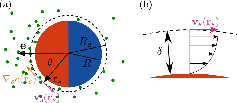
Figure 2: (a) Sketch of a Janus particle of radius $R$ with a catalytic cap (red) moving by self-diffusiophoresis. The particle creates a local concentration gradient of a solute, $\boldsymbol{\nabla}_{s}c(\mathbf{r}_{s})$, in tangential direction at position $\mathbf{r}_{s}$ and at a distance $\delta=R_{e}-R$ away from the particle surface. The surface velocity $\mathbf{v}_{s}$ is proportional to the concentration gradient. (b) Within the diffusive boundary layer of thickness $\delta$ a surface velocity field $\mathbf{v}_{s}$ develops, which depends on the position $\mathbf{r}_{s}$ at the surface.

2.2.1 Experimental realisations of active colloids

At present a variety of different active colloidal systems have been realized experimentally. Paxton et al. [6] and Fournier-Bidoz et al. [7] were the first to create micrometer-sized active bimetallic rods. They propel themselves by consuming fuel such as $\textrm{H}_{2}\textrm{O}_{2}$ at one end of the rod due to the different surface chemistry . Here, a local ion gradient creates an electric field, which initiates fluid flow close to the rod and hence electrophoretic self-propulsion. Spherical active colloids [43, 66] and sphere-dimers [75] are able to swim by self-diffusiophoresis, where a gradient in chemical species close to the surface generates a pressure gradient along the surface and thereby fluid flow [46].

Water droplets can become active and move in oil by consuming bromine fuel supplied inside the droplet. The bromination of mono-olein surfactants at the water-oil interface induces gradients in surface tension and thus Marangoni stresses, which initiate surface flow and thereby self-propulsion [8, 50, 77, 56]. Even pure water droplets are able to move by spontaneous symmetry breaking of the surfactant concentration at the interface [76] as do liquid-crystal droplets [56]. In both cases, surfactant micelles are crucial to initiate the spontaneous symmetry breaking [52].

When swimmers depend on fuel, they stop moving after it has been consumed. Instead of supplying fuel in the solution, permanent illumination with laser light as a power source can sustain self-propulsion for an arbitrarily long time. For example, in Refs. [45, 79] the authors suspend Janus particles with a golden cap in a water-lutidine mixture. Heating the cap with laser light demixes the binary liquid and initiates self-diffusiophoretic motion. Recent theoretical calculations have been performed in Refs. [80, 81].

Finally, the release of bubbles behind an active colloid [82, 83] or from cone-shaped microtubes [84, 85] can also lead to self-propulsion. Moreover, self-propelled colloids were designed that are powered by ultrasound [86].

Currently the number of experimentally realized colloidal swimmers is increasing fast. We refer to recent reviews, which also discuss more details of the different mechanisms for generating self-locomotion [24, 25, 26, 27, 28, 29, 4, 30, 31].

2.2.2 Theoretical description and modeling of self-phoretic swimmers

We discuss in more detail the concept of self-phoresis, by which solid active colloids move forward, and also comment on the Marangoni-propulsion of active emulsion droplets.

The gradient of an external field $X(\mathbf{r})$ induces phoretic transport of a passive colloid of radius $R$ since the field determines the interaction between the colloidal surface and the surrounding fluid [21]. Within a thin layer of thickness $\delta\ll R$ the field gradient $\boldsymbol{\nabla}X(\mathbf{r})$ induces a tangential near-surface flow, which increases from zero in radial direction and saturates at an effective radius $R_{e}=R+\delta$ to a constant value [see figure 2(b)]. Typically, the external field $X(\mathbf{r})$ is an electric potential $\phi(\mathbf{r})$, a chemical concentration field $c(\mathbf{r})$, or a temperature field $T(\mathbf{r})$ and the respective colloidal transport mechanisms are called electrophoresis, diffusiophoresis, and thermophoresis.

In contrast, active colloids create the local field gradient $\boldsymbol{\nabla}X(\mathbf{r})$ and the resulting near-surface flow by themselves. In the simplest case, half-coated Janus spheres are used as sketched in figure 2(a). The catalytic cap (red) catalyzes a chemical reaction of the fuel towards a chemical product (shown as green dots), which diffuses around. In steady state a non-uniform concentration profile around the particle is established [46, 47, 48, 87, 88, 89, 90, 91, 92, 93]. Since the Janus colloid produces the diffusing chemical by itself, the propulsion mechanism is called self-diffusiophoresis. Recent works showed how details of the surface coating and ionic effects determine the swimming speed and efficiency of catalytically driven active colloids [94, 95, 96, 65, 97, 92, 98].

Janus colloids coated with metals such as gold are able to move by heating the metal cap [44, 64, 99, 100, 101]. The resulting local temperature gradient induces an effective slip velocity, which is known as Soret effect, and the active colloid moves by self-thermophoresis. Furthermore, bimetallic nano- and microrods move by self-electrophoresis [102, 103, 104]. Here an ionic current near the surface drags fluid with it and thereby induces an effective slip velocity at the surface.

All the systems mentioned above create a tangential slip velocity $\mathbf{v}_{s}$ close to the particle surface and proportional to the field gradient $\boldsymbol{\nabla}_{s}X(\mathbf{r})$ along the surface [21],

$$\mathbf{v}_{s}(\mathbf{r}_{s})=-\kappa(\mathbf{r}_{s})\left.\boldsymbol{\nabla}_{s}X(\mathbf{r})\right|_{|\mathbf{r}|=R_{e}}\,.$$ (14)

The slip-velocity coefficient $\kappa$ depends on the specific phoretic mechanism and material properties of the particle-fluid interface, which vary with the location $\mathbf{r}_{s}$. For spherical active colloids with axisymmetric surface coating, $\mathbf{v}_{s}(\theta)$ depends on the polar angle $\theta$ of the position vector $\mathbf{r}_{s}$ relative to the orientation vector $\mathbf{e}$ [see figure 2(a)].

To determine the swimming speed and the flow field around the active colloid, one takes the slip velocity at the effective radius $R_{e}=R+\delta$. In concrete, one solves the homogeneous Stokes equations for $r>R_{e}$ with the boundary condition $\mathbf{u}(\mathbf{r}_{s})=\mathbf{v}_{s}+v_{0}\mathbf{e}+\boldsymbol{\Omega}\times\mathbf{r}_{s}$, where $v_{0}$ is the constant swimming speed and $\boldsymbol{\Omega}$ is the angular velocity of the active colloid. Since phoretic transport is force- and torque free [21], both the hydrodynamic force and torque of equations (3) and (4) should be zero when evaluated along the surface with radius $R_{e}$. This gives the translational and angular velocity of a spherical (self-)phoretic colloid [21],

$$\mathbf{V} =v_{0}\mathbf{e}=-\langle\mathbf{v}_{s}\rangle$$ (15)

$$\boldsymbol{\Omega} =-\frac{3}{2R}\langle\mathbf{v}_{s}\times\mathbf{n}\rangle\,,$$ (16)

where $\langle\cdots\rangle$ denotes the average taken over the surface with normal $\mathbf{n}$. Note that for axissymmetric surface velocity profiles, $\boldsymbol{\Omega}=\mathbf{0}$ and the active colloid moves on a straight line. This is, for example, true for half-coated Janus spheres. Nevertheless, rotational Brownian motion reorients the swimmer and it performs a persistent random walk, as we will discuss in section 3.1.

To gain a better insight into self-phoretic motion on the microscopic level, explicit hydrodynamic mesoscale simulation techniques have been used to study self-diffusiophoretic and self-thermophoretic motion. In particular, reactive multi-particle colision dynamics (R-MPCD) is a method to explicitely simulate the full hydrodynamic flow fields and chemical fields around a swimmer. It also includes chemical reactions between solutes and thermal noise [105]. The method was used to simulate the self-phoretic motion of spherical Janus colloids [106, 107] and self-propelled sphere dimers [74, 108, 109, 110, 75, 111, 112, 113, 107, 114]. The simulated flow field of a sphere-dimer swimmer agrees with that of a force dipole [115, 116], which has recently been confirmed by an analytic calculation [116]. Dissipative particle dynamics was used to determine the effect of particle shape on active motion [117], and to calculate the flow fields initiated by self-propelled Janus colloids for different fluid-colloid interactions [118].

In active emulsion droplets spontaneous symmetry breaking generates gradients in the density of surfactant molecules at the droplet-fluid interface and thus gradients in surface tension $\sigma$. They drive Marangoni flow at the interface [8, 50, 51, 76, 52]. The slip velocity field does not simply follow from an equivalent of equation (14), which links slip velocity to $\boldsymbol{\nabla}_{s}\sigma(\mathbf{r}_{s})$. Instead, one has to solve the Stokes equations inside and outside the droplets and match the difference in tangential viscous stresses by $\boldsymbol{\nabla}_{s}\sigma(\mathbf{r}_{s})$ [52]. So, in contrast to colloidal particles fluid flow also evolves inside the droplet [53, 55, 119, 8].

2.2.3 Swimming with prescribed surface velocity

We have seen that the active motion of self-phoretic colloids is mainly determined by the surface velocity field $\mathbf{v}_{s}$ independent of the underlying physical or chemical mechanisms to realize $\mathbf{v}_{s}$. In the simplest case one assumes a prescribed surface velocity field without taking the underlying mechanism into account. Such model swimmers are useful to study how hydrodynamic flow fields influence the (collective) dynamics of microswimmers.

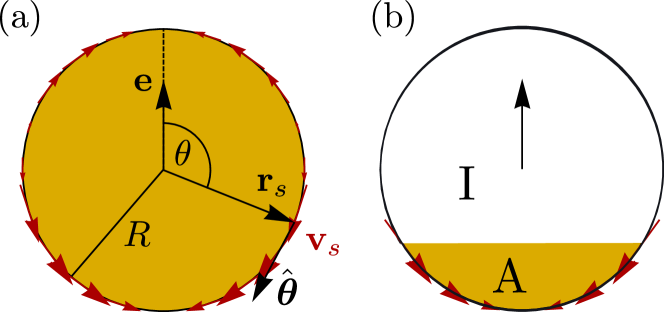
Figure 3: (a) Sketch of a spherical squirmer of radius $R$ swimming along direction $\mathbf{e}$. The axisymmetric surface velocity field $\mathbf{v}_{s}$ points along the tangential polar direction $\hat{\boldsymbol{\theta}}$ and depends on the position $\mathbf{r}_{s}$ on the surface, i.e., on the polar angle $\theta$. (b) Sketch of a simple model of an active Janus sphere, which is inert (I) at the front part and active (A) at the rear part.

One prominant example is the so-called squirmer [120, 121]. It was originally proposed to model ciliated microorganisms such as Paramecium and Opalina. Nowadays, the squirmer is frequently used as a simple model microswimmer. In its most common form, the squirmer is a solid spherical particle of radius $R$ with a prescribed tangential surface velocity field [122], which is expanded into an appropriate set of basis functions involving spherical harmonics [123, 52]. In the important case of an axisymmetric velocity field with only polar velocity component $v_{\theta}$, the expansion uses derivatives of Legendre polynomials $P_{n}(\cos\theta)$ [120, 121, 122],

$$v_{\theta} =\sum_{n=1}B_{n}\frac{2}{n(n+1)}\sin\theta\frac{dP_{n}(\cos\theta)}{d\cos\theta}$$ (17)

$$=B_{1}\sin\theta(1+\beta\cos\theta)+\dots$$ (18)

where the coefficients $B_{n}$ characterize the surface velocity modes and $\mathbf{v}_{s}=v_{\theta}\hat{\boldsymbol{\theta}}$ is directed along the longitudinals [see figure 3(a)]. We also introduced the dimensionless squirmer parameter $\beta=B_{2}/B_{1}$, which defines the strength of the second squirming mode relative to the first one. Without loss of generality we set $B_{1}>0$ and the squirmer swims into the positive $z$ direction as we will demonstrate below. Typically, only the first two modes are considered and $B_{n}=0$ for $n\geq 3$ [122, 124]. The reason is that $B_{1}$ and $B_{2}$ already capture the basic features of microswimmers. If $B_{1}$ is the only non-zero coefficient, the resulting flow field in the bulk fluid is exactly that of a source dipole and illustrated in figures 1(f). The coeffcient $B_{1}$ is linearly related to the source-dipole strength $q$ in equation (11), $q=8\pi\eta B_{1}R^{3}/3$. If we add the second mode, $B_{2}\neq 0$, the far field of the swimmer is that of a force dipole shown in figure 1(b). It decays more slowly with distance than the source dipole field. To match the boundary condition at the swimmer surface, an additional term $\propto r^{-4}$ is needed [122]. Figure 1(e) illustrates the complete squirmer flow field for a pusher with $\beta=-3$. The second mode coefficient $B_{2}$ is related to the force dipole strength $p$ introduced in equation (10) by $p=-4\pi R^{3}\eta B_{2}$. So, $B_{2}\propto\beta<0$ describes a pusher ($p>0$), while for $B_{2}\propto\beta>0$ the squirmer realizes a puller ($p<0$).

We note that a coordinate-free expression of the surface velocity field reads [122]

$$\mathbf{v}_{s} =\sum_{n=1}B_{n}\frac{2}{n(n+1)}[(\mathbf{e}\cdot\hat{\mathbf{r}})\hat{\mathbf{r}}-\mathbf{e}]\frac{dP_{n}(\mathbf{e}\cdot\hat{\mathbf{r}})}{d(\mathbf{e}\cdot\hat{\mathbf{r}})}$$ (19)

$$=B_{1}(1+\beta\mathbf{e}\cdot\hat{\mathbf{r}}_{s})[(\mathbf{e}\cdot\hat{\mathbf{r}}_{s})\hat{\mathbf{r}}_{s}-\mathbf{e}]+\dots\,,$$ (20)

where we introduced the the swimming direction $\mathbf{e}$ and the unit vector $\hat{\mathbf{r}}=\mathbf{r}/r$. We calculate the velocity of the squirmer by inserting equation (19) into equation (15) and obain $v_{0}=2B_{1}/3$. Hence, the swimming velocity only depends on the first mode $B_{1}$.

A simple model of an active Janus particle also uses a prescribed surface velocity field [see figure 3(b)]. While the inert part (I) of the particle surface fulfills the boundary condition of a passive colloid ($\mathbf{v}_{s}=0$), the chemically active cap (A) generates nearby slip flow and $\mathbf{v}_{s}\neq 0$ [62].

Noteworthy, numerical simulations were also performed with ellipsoidal and rodlike swimmers driven by a surface flow [125, 126, 127, 128, 129, 62, 130, 131].

2.3 Colloidal surfers and rollers

Some colloidal objects need bounding surfaces to move forward. For example, magnetically actuated colloidal doublet rotors perform non-reciprocal motion in the presence of solid surfaces, which leads to directed motion [132, 133]. Bricard et al. applied a static electric field between two conducting glass slides, while the lower slide was populated with sedimented insulating spheres [11]. At sufficiently high field strength the particles start to rotate about a random direction parallel to the surface. This is known as Quincke rotation, where the polarization axis rotates away from the field direction and thereby spontaneously breaks the axial symmetry [134, 135, 136, 11]. The well-known translational-rotational coupling of a spherical colloid close to a no-slip surface then induces directed motion [58, 137]. Its well-defined velocity depends on the electric field strength, $v_{0}\sim[(E/E_{Q})^{2}-1]^{1/2}$, where $E_{Q}$ is the critical field strength for the Quincke rotation to set in. Note that this rolling motion was already observed and explained by Jákli et al. [137], who investigated Quincke rotation in liquid crystals [138, 137].

Palacci et al. studied the motion of colloidal surfers [10, 139]. They consist of a photoactive material (e.g. hematide) embedded in polymer spheres, which are dispersed in a solvent containing $\textrm{H}_{2}\textrm{O}_{2}$. After sedimenting to the lower substrate, the particles are illuminated by UV light. The photoactive material triggers the dissoziation of $\textrm{H}_{2}\textrm{O}_{2}$, which generates osmotic flow along the substrate. This rotates the active part towards the substrate and the particles start moving. Although the exact swimming mechanism is not known yet, the substrate and the osmotic flow are necessary for self-propulsion [10, 139].

2.4 Active Brownian particles

Modeling the motion of biological and artificial microswimmers has become a largely growing field in statistical physics, hydrodynamics, and soft matter physics. A minimal model for microswimmers and other active individuals are active Brownian particles [140, 2, 3]. They only capture the very basic features of active motion: (i) overdamped dynamics of particle position $\mathbf{r}$ and particle orientation $\mathbf{e}$, (ii) motion with intrinsic particle velocity $v_{0}$ along the direction $\mathbf{e}$, and (iii) thermal (and non-thermal) translational as well as rotational noise, $\boldsymbol{\xi}$ and $\boldsymbol{\xi}_{r}$. The motion of spherical (see, for example, [141, 142, 143, 71, 144, 145, 12, 146, 147, 148, 149, 150, 151, 152, 153, 154, 155]), elongated (see, for example, [156, 157, 158, 159, 160, 142, 161, 162, 163]), and active Brownian particles with more complex shapes [164, 165, 166, 167] has extensively been studied.

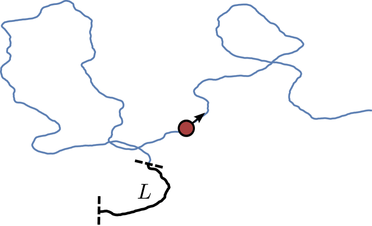
Figure 4: Example trajectory of active Brownian motion. The persistence length $L$ defines the typical distance over which the active particle has lost information about its initial orientation. In units of the swimmer diameter it is called persistence number, see equation (28).

The most important example is the overdamped motion of an active Brownian sphere. The dynamics for its position $\mathbf{r}(t)$ and orientation $\mathbf{e}(t)$ is determined by the Langevin equations

$$\dot{\mathbf{r}} =v_{0}\mathbf{e}+\sqrt{2D}\boldsymbol{\xi}$$ (21)

$$\dot{\mathbf{e}} =\sqrt{2D_{r}}\boldsymbol{\xi}_{r}\times\mathbf{e}\,,$$ (22)

where $D$ is the translational and $D_{r}$ the rotational diffusion constant of a sphere. The rescaled stochastic force $\boldsymbol{\xi}$ and torque $\boldsymbol{\xi}_{r}$ fulfill the conditions for delta-correlated Gaussian white noise,

$$\langle\boldsymbol{\xi}(t)\rangle=0\enspace,\enspace\langle\boldsymbol{\xi}(t)\otimes\boldsymbol{\xi}(t^{\prime})\rangle=\textbf{{1}}\delta(t-t^{\prime})$$ (23)

and

$$\langle\boldsymbol{\xi}_{r}(t)\rangle=0\enspace,\enspace\langle\boldsymbol{\xi}_{r}(t)\otimes\boldsymbol{\xi}_{r}(t^{\prime})\rangle=\textbf{{1}}\delta(t-t^{\prime})\,.$$ (24)

The unit vector $\mathbf{e}$ performs a random walk on the unit sphere (3D) or unit circle (2D). A typical spatial trajectory in 2D is shown in figure 4.

3 Generic Features of Single Particle Motion

In the following we discuss generic features of active motion, which already reveal themselves for single active colloids.

3.1 Persistent Random Walk

Beside their directed swimming motion, active colloids also perform random motion due to the presence of noise as discussed in section 2.4. This leads to a persistent random walk, which is described by an effective diffusion constant on sufficiently large length scales. We summarize the basic theory in the following. We use the Langevin equations (21) and (22) of an active Brownian particle that moves with constant speed $v_{0}$ and changes its orientation $\mathbf{e}(t)$ stochastically. Together with equations (24) characterizing rotational noise, the orientational time correlation function can be computed [59],

$$\langle\mathbf{e}(t)\cdot\mathbf{e}(0)\rangle=e^{-t/\tau_{r}}\,,$$ (25)

where $\tau_{r}$ is the orientational correlation time or persistence time. It quantifies the time during which the swimmer’s orientations are correlated. The persistence time is proportional to the inverse rotational diffusion constant $D_{r}$ and for a spherical particle becomes

$$\tau_{r}=\frac{1}{(d-1)D_{r}}\,,$$ (26)

where $d$ is the spatial dimension of the rotational motion. For pure thermal motion $D_{r}=k_{B}T/(8\pi\eta R^{3})$ and strongly depends on the radius $R$ of the particle. Note that the translational diffusion constant of a sphere is $D=k_{B}T/(6\pi\eta R)$ [59].

To quantify the importance of translational and rotational diffusion compared to the directed swimming motion, we define the active Péclet number Pe and the persistence number $\textrm{Pe}_{r}$, respectively. To do so, we introduce the ballistic time scale $t_{0}=2R/v_{0}$, which the microswimmer needs to swim its own diameter $2R$, and the diffusive time scale $t_{D}=4R^{2}/D$, which it needs to diffuse its own size. The Péclet number compares the two time scales,

$$\textrm{Pe}=\frac{t_{D}}{t_{0}}=\frac{2Rv_{0}}{D}.$$ (27)

For $\textrm{Pe}\ll 1$ the particle motion is mainly governed by translational diffusion, such as for passive Brownian particles, while for $\textrm{Pe}\gg 1$ diffusive transport is negligible compared to active motion.

The persistence number compares the persistence time $\tau_{r}$ to the ballistic time scale $t_{0}$,

$$\textrm{Pe}_{r}=\frac{\tau_{r}}{t_{0}}=\frac{v_{0}}{2RD_{r}}=\frac{v_{0}\tau_{r}}{2R}=\frac{L}{2R},$$ (28)

where $L=v_{0}\tau_{r}$ is the persistence length, i.e., the distance a swimmer moves approximately in one direction. Thus, $\textrm{Pe}_{r}$ measures the persistence length in units of the particle diameter [168, 169, 170, 171]. Note that for purely thermal noise,

$$D_{r}=\frac{3D}{4R^{2}}\quad\mathrm{and}\quad\textrm{Pe}_{r}=\frac{\textrm{Pe}}{3}\,.$$ (29)

Non-thermal rotational noise, however, can significantly decrease the persistence of the swimmer [43, 44] such that $\textrm{Pe}_{r}\leq\textrm{Pe}/3$. Typical values for Pe and $\textrm{Pe}_{r}$ for spherical micron-sized active colloids are of the order $10^{0}-10^{2}$ [43, 44, 66, 79, 10]. In figure 4 a typical persistence length of the random walk of a spherical microswimmer in 2D is indicated.

We now discuss the mean square displacement of the active particle, which defines an effective diffusion coefficient $D_{\mathrm{eff}}$. The persistent random walk of active particles was first formulated by R. Fürth in 1920 and also experimentally verified with Paramecia and an unknown species [172]. Using equations (21)–(24) the mean square displacement $\langle\Delta r^{2}(t)\rangle=\langle|\mathbf{r}(t)-\mathbf{r}(0)|^{2}\rangle$ can be calculated as [43, 124, 142]

$$\langle\Delta r^{2}(t)\rangle=2dDt+2v_{0}^{2}\tau_{r}t-2v_{0}^{2}\tau_{r}^{2}(1-e^{-t/\tau_{r}})\,.$$ (30)

For times small compared to the persistence time, $t\ll\tau_{r}$, equation (30) reduces to

$$\langle\Delta r^{2}(t)\rangle=v_{0}^{2}t^{2}+2dDt,$$ (31)

which includes contributions from the ballistic motion of the swimmer and from translational diffusion. However, for $t\gg\tau_{r}$ the swimmer orientation decorrelates from its initial value and the active colloid performs diffusive motion,

$$\langle\Delta r^{2}(t)\rangle=(2dD+2v_{0}^{2}\tau_{r})t=2dD_{\mathrm{eff}}t,$$ (32)

with the effective diffusion constant

$$D_{\mathrm{eff}}=D+\frac{1}{d}v_{0}^{2}\tau_{r}=D+\frac{v_{0}^{2}}{d(d-1)D_{r}}\,.$$ (33)

For pure thermal noise, using equations (29) and $d=3$, it can be rewritten either with the persistence number $\textrm{Pe}_{r}$ or the Péclet number Pe,

$$D_{\mathrm{eff}}=D(1+2\textrm{Pe}_{r}^{2})=D(1+\frac{2}{9}\textrm{Pe}^{2})$$ (34)

Hence, $D_{\mathrm{eff}}$ quadratically increases with Pe. Note that $D_{\mathrm{eff}}$ can also be calculated via the velocity-autocorrelation function using the corresponding Green-Kubo relation [4].

3.2 Motion under gravity

When the density of the active colloid $\rho_{c}$ is larger than the density of the surrounding medium $\rho_{f}$, it sediments in the gravitational field $\mathbf{g}=-g\hat{\mathbf{z}}$. The active colloid experiences a sedimentation force $\delta m\mathbf{g}\sim(\rho_{c}-\rho_{f})\mathbf{g}=const$, where $\delta m$ is the buoyant mass of the active colloid and $g=9.81m/s$. The Langevin equation for the position of the sedimenting active colloid reads

$$\dot{\mathbf{r}}=v_{0}\mathbf{e}+(\delta m/\gamma)\mathbf{g}+\sqrt{2D}\boldsymbol{\xi}_{1}\,.$$ (35)

Alteratively, one formulates the Smoluchowski equation for the propability distribution $\rho(\mathbf{r},\mathbf{e},t)$ for position and orientation [173, 174],

$$\frac{\partial\rho}{\partial t}+\nabla\cdot\mathbf{J}^{\mathrm{trans}}+\mathcal{R}\cdot\mathbf{J}^{\mathrm{rot}}=0\,,$$ (36)

with the respective translational and rotational currents

$$\mathbf{J}^{\mathrm{trans}}=-D\nabla\rho+\left(v_{0}\mathbf{e}+\delta m\mathbf{g}/\gamma\right)\rho\enspace,\enspace\mathbf{J}^{\mathrm{rot}}=-D_{r}\mathcal{R}\rho\,.$$

The latter is purely diffusive with the rotational operator $\mathcal{R}=\mathbf{e}\times\nabla_{\mathbf{e}}$.

A multipole expansion of $\rho$ gives an exponential sedimentation profile for the spatial density, as for passive particles,

$$\rho_{0}(z)=\rho_{0}(0)\exp(-z/\delta_{\mathrm{eff}})\,.$$ (37)

However, the sedimentation length [175, 176, 66, 173, 177]

$$\delta_{\mathrm{eff}}=\delta_{0}\left(1+\frac{2\textrm{Pe}^{2}}{9}\right)=\frac{\delta_{0}D_{\mathrm{eff}}}{D}$$ (38)

is increased compared to the passive case with $\delta_{0}=k_{B}T/(mg)$. This can also be rationalized by introducing an increased effective temperature $T_{\mathrm{eff}}=TD_{\mathrm{eff}}/D$ [66]. Clearly, the larger sedimentation length is due to the larger effective diffusion of active particles. However, the deeper reason is that they develop polar order by aligning against the gravitational field [173].

Gravitaxis of spherical active colloids with asymmetric mass distribution was observed in experiments [178] and described theoretically [174]. Interestingly, the interplay of gravity and intrinsic circling motion of asymmetric L-shaped active colloids [165] leads to various complex swimming paths and gravitaxis, induced by the shape asymmetry [167].

3.3 Taxis of active colloids

Taxis means the ability of biological microswimmers such as bacteria or sperm cells to move along field gradients. For example, gradients of a chemical field or a light intensity field can initiate chemotaxis [179] or phototaxis [180], respectively. We already mentioned that colloids also react to field gradients, which generate phoretic transport. Combined with activity, one obtains artificial microswimmers that can mimic biological taxis. Here we discuss how active colloids move in field gradients $\boldsymbol{\nabla}X(\mathbf{r})$ that are (i) externally applied such as in classical phoretic transport, (ii) generated by other self-phoretic active colloids, or (iii) generated by the active colloid itself and therefore known as autochemotaxis.

3.3.1 Motion in external field gradients

Self-phoretic active colloids are surrounded by a cloud of self-generated field gradients but also respond to external gradients $\boldsymbol{\nabla}X(\mathbf{r})$. Again, this can be realized by diffusio-, electro-, or thermophoresis. Then, spherical colloids at position $\mathbf{r}$, either passive or active, translate with velocity $\mathbf{U}_{C}$ and rotate with angular velocity $\boldsymbol{\Omega}_{C}$ [21],

$$\mathbf{U}_{C} =\Big{[}\langle\kappa(\mathbf{r}_{s})\rangle\mathbf{1}-\frac{1}{2}\langle(3\mathbf{n}\otimes\mathbf{n}-\mathbf{1})\kappa(\mathbf{r}_{s})\rangle\Big{]}\boldsymbol{\nabla}X(\mathbf{r})\,,$$ (39)

$$\boldsymbol{\Omega}_{C} =\frac{9}{4R}\langle\mathbf{n}\kappa(\mathbf{r}_{s})\rangle\times\boldsymbol{\nabla}X(\mathbf{r})\,,$$ (40)

where $\kappa(\mathbf{r}_{s})$ is the slip-velocity coefficient introduced in equation (14) and $\langle\ldots\rangle$ is again the average taken over the particle surface with normal $\mathbf{n}$. Finally, the total colloidal velocity reads $\mathbf{U}=v_{0}\mathbf{e}+\mathbf{U}_{C}$, and the angular velocity is simply $\boldsymbol{\Omega}=\boldsymbol{\Omega}_{C}$. This is sketched in figure 5. Note, however, that the velocity $v_{0}$ will in general depend on the local concentration $X(\mathbf{r})$ [181].

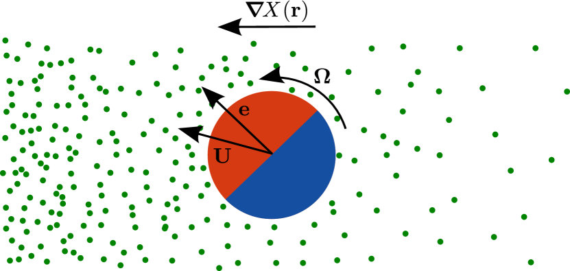
Figure 5: An active colloid moving in an external field gradient $\boldsymbol{\nabla}X(\mathbf{r})$. Due to phoresis its velocity $\mathbf{U}=v_{0}\mathbf{e}+\mathbf{U}_{C}$ is not parallel to its intrisic symmetry axis $\mathbf{e}$ and it rotates with angular velocity $\boldsymbol{\Omega}\neq\textbf{0}$.

Experimentally, the chemotactic response of active Janus colloids in a concentration gradient $\boldsymbol{\nabla}c(\mathbf{r})$ of $\textrm{H}_{2}\textrm{O}_{2}$ was observed [182, 183, 184, 185, 186, 187, 188, 30]. A self-propelled nano-dimer motor moving in a chemical gradient was simulated in Ref. [189]. Recent studies on interacting self-phoretic active colloids (see chapter 4) considered phoretic attraction and repulsion but also reorientation of a particle due to field gradients produced by others [9, 10, 181, 190, 191, 192, 193].

3.3.2 Autochemotaxis

The chemical field $c(\mathbf{r},t)$, which a self-diffusiophoretic particle creates, diffuses on the characteristic time scale $t_{c}\propto D_{c}^{-1}R^{2}$, where $D_{c}$ is the diffusion constant of the chemical species and $R$ is the particle radius. Since the chemical diffuses fast, one typically has $t_{c}\ll\tau_{r}$, where $\tau_{r}$ is the orientational persistence time introduced in section 3.1. The particle interacts with its own chemical trail, which is known as autochemotaxis. Thus, the chemical field couples back to the motion of the microswimmer, which can drastically modify its ballistic and diffusive movement. The implications were mainly studied in the context of biological autochemotactic systems [194, 195, 196, 171, 197] and recently discussed for active colloids [48].

In Ref. [48] the interaction of an active colloid with its self-generated chemical cloud was investigated. Since the active colloid performs rotational diffusion and the released product molecules at the chemically active surface diffuse on a finite time $t_{c}$, a non-stationary concentration profile around the particle evolves. As a result, the mean square displacement of equation (30) is modified and shows anomalous diffusion at intermediate time scales and a modified effective diffusion in the long-time limit [48].

3.4 Motion in external fluid flow

Biological microswimmers have to respond to fluid flow in their natural environments [198]. In addition, we expect that in the near future new experiments and simulations on the motion of active colloids in microchannel flows will be performed. Finally, one has the vision that articial microswimmers may be used in the future to navigate through human blood vessels [199].

Here we discuss the basic physical mechanisms for microswimmers such as active colloids moving in fluid flow. We consider an axisymmetric active particle with orientation $\mathbf{e}$ that swims in a background flow field $\mathbf{u}(\mathbf{r},t)$ at low Reynolds number. This problem was first formulated for biological microswimmers by J O Kessler and T J Pedley (see, e.g., [200] for a review). If variations of the flow field on the size of the particle are small, a passive particle simply acts as a tracer particle and follows the stream lines of the flow. Thus its velocity is $\mathbf{u}(\mathbf{r}(t))$, where $\mathbf{r}(t)$ denotes the center-of-mass position of the particle. For an active particle one has to add the swimming velocity and the total particle velocity becomes $\mathbf{V}=v_{0}\mathbf{e}+\mathbf{u}(\mathbf{r}(t))$. We assume a constant intrisic particle speed $v_{0}$, which is not altered by the presence of the flow. The particle orientation $\mathbf{e}$, however, changes continuously in fluid flow. For a spherical particle Faxéns second law determines the angular velocity as $\boldsymbol{\Omega}=\frac{1}{2}\boldsymbol{\nabla}\times\mathbf{u}$ proportional to the local vorticity of $\mathbf{u}(\mathbf{r})$ [59]. For an elongated ellipsoid of length $L$ and width $W$ the angular velocity is modified to

$$\boldsymbol{\Omega}=\frac{1}{2}\boldsymbol{\nabla}\times\mathbf{u}+G\mathbf{e}\times\textsf{E}\,\mathbf{e}\,,$$ (41)

where E is the strain rate tensor and $G=(\gamma^{2}-1)/(\gamma^{2}+1)\in[0,1)$ is a geometrical factor related to the aspect ratio of the swimmer, $\gamma=L/W$. At low Reynolds number the equations of motions are overdamped [200] and they read

$$\dot{\mathbf{r}}=v_{0}\mathbf{e}+\mathbf{u}\quad\mathrm{and}\quad\dot{\mathbf{e}}=\boldsymbol{\Omega}\times\mathbf{e}\,.$$ (42)

The solutions of the second equation for the deterministic rotation of an axisymmetric passive particle in shear flow are known as Jeffery orbits named after G B Jeffery [201]. The orientation vector $\mathbf{e}$ moves on a periodic orbit on the unit sphere, where the specific solution $\mathbf{e}(t)$ depends on the Jeffery constant, which is a constant of motion of the second equation in (42).

To demonstrate basic features of the problem, we focus here on a spherical active particle without noise moving in two dimensions in a steady unidirectional flow field $\mathbf{u}=u_{z}(x)\hat{\mathbf{z}}$. As sketched in figures 6(a,b), the swimmer moves in the $x$-$z$ plane and its orientation is described by the angle $\Psi$. The equations of motion (42) then simplify to [200, 202, 143, 203, 204]

$$\dot{\Psi} =-\frac{1}{2}\partial_{x}u_{z}(x),$$ (43)

$$\dot{x} =-v_{0}\sin\Psi,$$ (44)

$$\dot{z} =-v_{0}\cos\Psi+u_{z}(x).$$ (45)

Since only equations (43) and (44) are coupled and do not depend on $z$, one first considers the solutions in $x$-$\Psi$ space. Once $x(t)$ and $\Psi(t)$ are known, they can be inserted into equation (45) to determine $z(t)$ by integration.

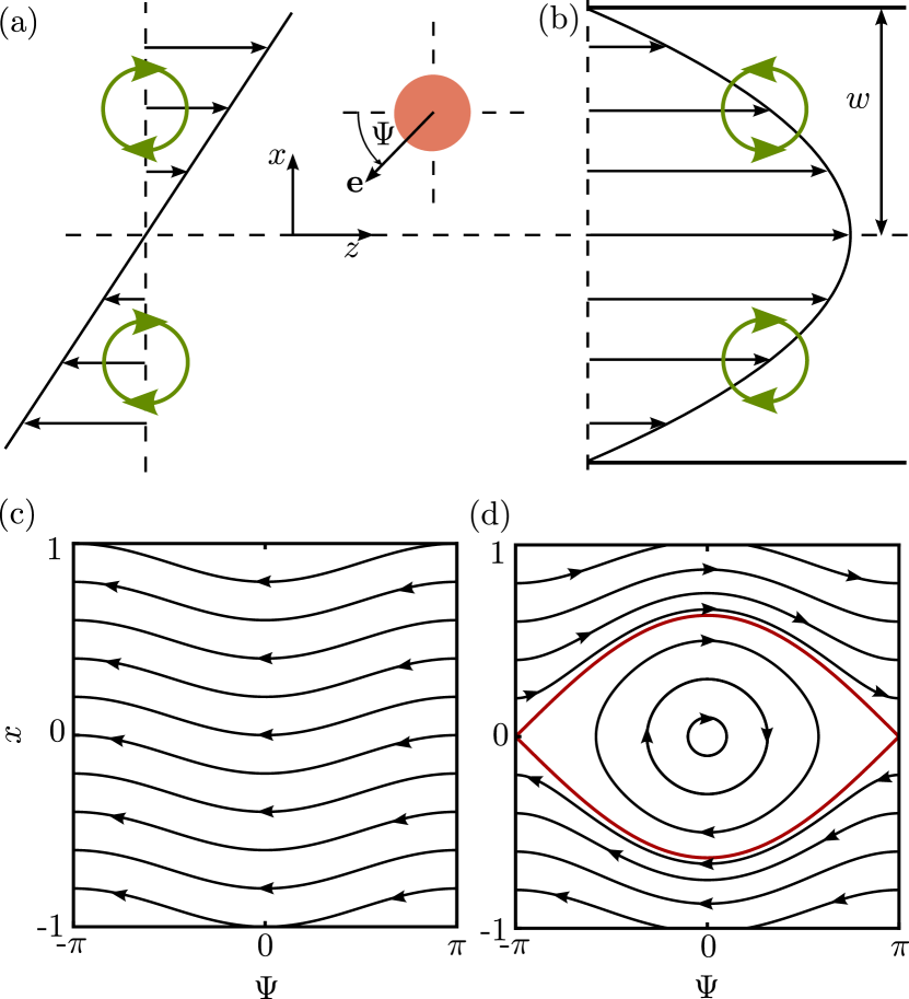
Figure 6: A swimmer with lateral position $x$ and orientation angle $\Psi$ moves along planar trajectories in (a) simple shear flow and (b) Poiseuille flow. The flow vorticities are indicated in green. The corresponding phase portraits or trajectories in $x$-$\Psi$ phase space are shown in (c) for shear flow and in (d) for Poiseuille flow.

For example, in simple shear flow, $\mathbf{u}=\dot{\Gamma}x\hat{\mathbf{z}}$, where $\dot{\Gamma}=\textrm{const}$ is the shear rate [see also figure 6(a)], a spherical swimmer tumbles with a constant angular velocity $\dot{\Psi}=-\dot{\Gamma}/2$ and it moves on a cycloidic trajectory [143]. The corresponding phase portrait in $x$-$\Psi$ space is shown in figure 6(c). Since the angular velocity $\dot{\Psi}$ of the swimmer is independent of $x$, all starting positions $x(0)$ initiate the same cycloidic trajectory.

The situation is more complex in pressure-driven planar Poiseuille flow in a channel of width $2w$. The flow field becomes $\mathbf{u}=v_{f}(1-x^{2}/w^{2})\hat{\mathbf{z}}$, where $v_{f}$ is the flow speed in the center of the channel [see also figure 6(b)]. Here the angular velocity $\dot{\Psi}=v_{f}x/w^{2}$ of the swimmer is linear in the lateral position $x$ in the channel. When the swimmer starts sufficiently far away from the centerline or oriented downstream, it does not cross the centerline and again tumbles in flow but with non-constant angular velocity. In contrast, when the swimmer starts oriented upstream and sufficiently close to the centerline, flow vorticity rotates it towards the center of the channel, it crosses the centerline, the flow vorticity changes sign, and the swimmer changes its sense of rotation, and is again directed towards the centerline. This results in an upstream-oriented swinging motion around the centerline. For small amplitudes the frequency becomes $\omega=(v_{0}v_{f}/w^{2})^{1/2}$ [203]. It depends on the swimming speed and flow curvature $2v_{f}/w^{2}$. The dependence on flow speed $v_{f}$ has recently been confirmed in experiments with a biological microswimmer called African trypanosome [205].

In figure 6(d) swinging and tumbling trajectories are represented in $x$-$\Psi$ phase space. They are divided by a separatrix shown in red. The equations of motion (43) and (44) for swimming in Poiseuille flow are formally the same as for the mathematical pendulum. In particular, they can be combined to $\ddot{\psi}+\omega^{2}\sin\psi=0$ with $\omega$ given above. Thus the oscillating and circling solutions of the pendulum correspond to the swinging and tumbling trajectories of the swimmer, respectively.

Due to the formal correspondence with the pendulum, the system also possesses a Hamiltonian $H$. It consists of a potential energy, depending on the angle $\Psi$, and a kinetic energy, depending on the position $x$, which formally plays the role of a velocity [203]. The existence of a Hamiltonian implies time-reversal symmetry and reflects the fact that the trajectories do not converge to stable solutions, i.e., active particles do not cluster at specific lateral positions or focus in flow. Only when time-reversal symmetry is broken, for example, in the presence of swimmer-wall hydrodynamic interactions [203], bottom-heaviness [206], phototaxis [207, 208], flexible body shape [209], or viscoelastic flows [210], does the dynamics become dissipative in the sense of dynamical systems and particles aggregate at specific locations in the flow. Although swinging and tumbling trajectories in microchannel Poiseuille flow have been observed experimentally with biological microswimmers [205, 211], they have not yet been confirmed in experiments with active colloids. Spherical and elongated swimmers moving in three dimensions in channels with elliptic cross sections still show swinging-like and tumbling-like trajectories, which can become quasi-periodic [204] or even chaotic [212].

We also note that the simple model equations (42) only capture the basic features of swimming active particles in flow. For example, adding thermal noise destroys the periodicity of the solutions and swinging and tumbling trajectories become stochastic [211, 213]. Swimmers are even able to cross the separatrix and switch between the two swimming modes [203]. Furthermore, the dynamics is altered when the flow field couples to the chemical field, which a self-phoretic particle generates around itself [110, 214, 215]. This becomes even more complicated in the presence of bounding surfaces [203, 216, 215, 217], where active colloids can swim stable against the flow and show rheotaxis [215, 217]. Finally, deformable active particles such as active droplets in flow also show complex swimming trajectories [218].

3.5 Motion near surfaces

Recently, studying the motion of active colloids in the vicinity of flat or curved surfaces came into focus [45, 62, 219, 220, 221, 222, 223, 224, 225, 226, 227, 228, 229, 230]. Confinement is usually implemented in experiments by using flat walls [45, 219], walls with edges [230], patterned surfaces [45], or passive colloids, which act as curved walls [221, 224].

A key feature of active particles is that they accumulate at surfaces even in the absence of electrostatic or other attractive swimmer-wall interactions, in contrast to passive particles. The accumulation of biological swimmers confined between two walls was first observed by Sir Rothschild with living sperm cells [231], and later by other researchers using swimming bacteria [232, 169, 233]. Active particles accumulate at walls, since they need some time, after colliding with a surface, to reorient away from the surface until they can escape [169, 173, 220, 225]. This is sketched in figure 7(a).

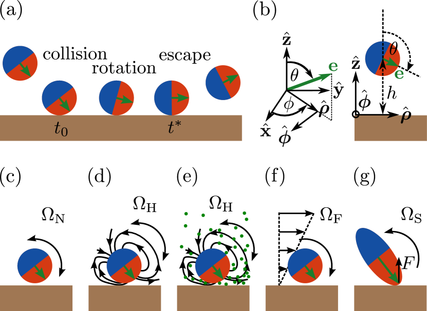
Figure 7: (a) Collision of an active colloid with a surface: Collision at time $t_{0}$, reorientation close to the wall, and escape from the wall at time $t^{\ast}$. (b) Definition of the coordinate system for an active colloid swimming in front of a wall: distance from the wall $h$, and orientation to the wall $\theta$. (c)-(g) Reorientation mechanisms close to the wall contributing to its angular velocity $\Omega_{W,\phi}=\dot{\theta}$: Rotational noise $\Omega_{N}$ (c), hydrodynamic swimmer-wall interactions $\Omega_{H}$ (d) which can depend on the chemical field $c(\mathbf{r})$ (e), external fluid flow $\Omega_{F}$ (f), and steric interactions $\Omega_{S}$ (g).

An axisymmetric Brownian microswimmer moves in bulk along its director $\mathbf{e}$. In the absence of any intrinsic or extrinsic torques acting on $\mathbf{e}$, the swimming direction only rotates due to rotational noise $\boldsymbol{\Omega}_{N}=\sqrt{2D_{r}}\boldsymbol{\xi}_{r}$ and its dynamics is determined by the Langevin equations (21) and (22). The presence of a surface alters the dynamics of the swimmer, which can be summarized by adding a wall-induced velocity $\mathbf{v}_{W}$ and a wall-induced angular velocity $\boldsymbol{\Omega}_{W}$ to equations (21) and (22), respectively. A spherical swimmer in front of a flat wall and the relevant polar coordinate system to express the orientation vector $\mathbf{e}=e_{\rho}\hat{\boldsymbol{\rho}}+e_{\phi}\hat{\boldsymbol{\phi}}+e_{z}\hat{\mathbf{z}}$ are shown in figure 7(b). Noise alters all components of the orientation and position vectors of the swimmer according to the modified Langevin equations (21) and (22), as before. Due to the axial symmetry, deterministic contributions to the drift velocities $\mathbf{v}_{W}$ and $\boldsymbol{\Omega}_{W}$ only depend on the distance $h$ of the swimmer from the wall and on the polar angle $\theta$ between the swimmer orientation and the wall normal. So, one has $\mathbf{v}_{W}=v_{W,\rho}(h,\theta)\hat{\boldsymbol{\rho}}+v_{W,z}(h,\theta)\hat{\mathbf{z}}$ and $\boldsymbol{\Omega}_{W}=\Omega_{W,\phi}(h,\theta)\hat{\boldsymbol{\phi}}$.

The reasons for the wall-induced translational and angular velocities depend on the specific properties of the swimmer, the wall, and the fluid. In figure 7(c)-(g) we sketch important mechanisms for active colloids to reorient close to the wall with angular velocity $\Omega_{W,\phi}=\dot{\theta}$.

First, rotational noise causes the angular velocity $\Omega_{N}=\sqrt{2D_{r}}\xi_{r}+D_{r}\cot\theta$, where $\xi_{r}$ is again Gaussian white noise [see equation (24)], and $D_{r}$ is the rotational diffusion constant close to the wall, which in general depends on $h$ [234]. The effective rotational drift term $D_{r}\cot\theta$ results from the Stratonovich interpretation of equation (22) with its multiplicative noise and ultimately appears since $\mathbf{e}$ performs random motion on the unit sphere [235, 236, 225]. The distribution of active Brownian particles confined between two parallel plates was studied by solving the corresponding Smoluchowski equation [220] and also in combination with gravity [173, 174].

Second, in order to fulfill the appropriate boundary condition at the wall, the fluid flow around the microswimmer is modified compared to the bulk solutions discussed in section 2.1. The resulting hydrodynamic swimmer-wall interactions are responsible for a hydrodynamic attraction/repulsion quantified by $\mathbf{v}_{W}$ and the reorientation rate $\Omega_{H}$ of the microswimmer in front of a slip- or no-slip wall [232, 237, 62, 225, 63] [see figure 7(d)]. In particular, for generic pusher and pullers explicit expressions for $\mathbf{v}_{W}$ and $\Omega_{H}$ exist based on their flow fields given in equation (10). While pushers have a stable orientation parallel to the wall, pullers are oriented perpendicular to bounding surfaces [232, 225]. Hydrodynamic interactions of the model swimmer squirmer (introduced in section 2.2.3) with a wall have recently been studied by several research groups [238, 239, 240, 62, 203, 241, 242, 243, 244, 245, 246, 247]. In contrast to far-field hydrodynamic swimmer-wall interactions, we observed that in lubrication approximation the force-dipole contribution of squirmer pullers to $\Omega_{H}$ behaves like the reorientation rate induced by a generic pusher (and vice versa). We mentioned this fact in Ref. [225] and in the Supplemental Material of Ref. [154] based on calculations from Ref. [122]. We note that bounding surfaces also alter the concentration of chemical fields around self-phoretic swimmers since the no-flux boundary condition at the wall has to be fulfilled. This changes the concentration gradient near the active colloid and thereby the driving surface velocity field, which in turn determines the flow field and hence the hydrodynamic swimmer-wall interactions [222, 228, 229] [see figure 7(e)].

Third, external fluid flow such as shear flow close to the wall induces an additional reorientation rate $\Omega_{F}$ as illustrated in figure 7(f). This rotates microswimmers preferentially against the flow resulting in a net upstream motion near walls in combination with hydrodynamic swimmer-wall interactions [248, 249, 250, 203, 216]. Finally, external flow can also alter the driving surface velocity field of active particles and the concentration of chemicals used to propel them [214, 215].

Forth, elongated swimmers that collide with a bounding surface tend to align with it due to steric interactions [159, 169, 160]. Upon collision a force acts from the wall on the front of the particle. The resulting torque rotates the swimmer with an angular velocity $\Omega_{S}(\theta)$ until it is parallel to the wall [169] [see figure 7(g)].

In the absence of noise stable swimming close to the wall is possible, either with a fixed orientation angle $\theta_{S}$ [251, 232, 222, 225] or performing (meta-)stable oscillations in $h$-$\theta$ configuration space close to the surface [252, 239, 244, 245]. It is also possible that a swimmer orients perpendicular to the wall and gets stuck there as noiseless generic pullers [232, 225] or active Janus particles with large caps [222, 228] would do. However, a real microswimmer always experiences thermal (and non-thermal) translational and rotational noise and therefore can escape from the wall as sketched in figure 7(a).

As a simple example we consider an active Brownian sphere with radius $R$. Its dynamics in front of a wall is governed by equations (21) and (22), where hydrodynamic and other swimmer-wall interactions are neglected. In addition, its dynamics is restricted to $z\geq R$. The particle hits the wall at an incoming orientation angle $\theta_{0}$ at time $t_{0}$ [see also figure 7(a)]. At the micron scale the Péclet number is often much larger than one meaning that translational diffusion is negligible against the active swimming motion and the active particle swims at the surface with $h(t)\approx R$. It can only escape from the wall when rotational noise drives the particle’s orientation to an escape angle $\theta^{\ast}=\pi/2$, where it can swim away from the wall at time $t^{\ast}$. The total time $t=t^{\ast}-t_{0}$ the active sphere stays at the surface is then called detention time [225], retention time [226], residence time [223], escape time [237], trapping time [221], or contact time [45] and is a stochastic variable. Its distribution $f(t|\theta_{0})$, which we call detention time distribution in [225], depends on the incoming angle $\theta_{0}$ and on the rotational diffusion constant $D_{r}$ near the wall. It can be calculated using the theory of first passage times. The mean detention time $T=\int_{0}^{\infty}tf(t|\theta_{0})dt$ of the active Brownian particle at the surface decreases linearly with $D_{r}$ [225],

$$T^{\mathrm{ABP}}=\frac{1}{D_{r}}\ln(1-\cos\theta_{0}).$$ (46)

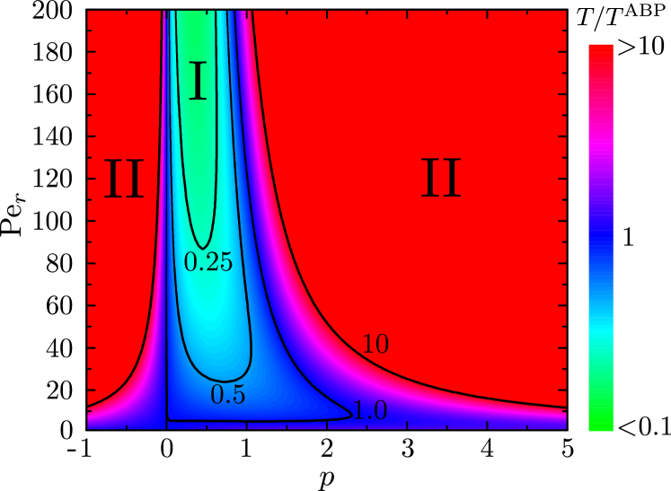
Figure 8: Mean detention times $T/T^{\mathrm{ABP}}$ for pushers ($p>0$) and pullers ($p<0$) depending on the force dipole strength $p$ and the persistence number $\mathrm{Pe}_{r}$. The incoming angle is $\theta_{0}=3\pi/4$. In region I $T/T^{\mathrm{ABP}}<1$, wheras in region II $T/T^{\mathrm{ABP}}\gg 1$. (Adapted from Ref. [225]; copyright (2015) American Physical Society).

Simple model pushers and pullers are hydrodynamically trapped at surfaces but can escape through rotational noise. Their mean detention times $T(p,\textrm{Pe}_{r})$ compared to $T^{\mathrm{ABP}}$ are shown in figure 8. For large persistence numbers $\mathrm{Pe}_{r}$ and sufficiently large force dipole strength $|p|$ (region II in figure 8), the escape from the surface can be mapped onto the escape of a particle over a large potential barrier $\Delta U$ (in our case the hydrodynamic torque potential) and the mean detention times are approximated by Kramers-like formulas, $T\sim e^{\Delta U/D_{r}}$ [237, 225]. Interestingly, for sufficiently small dipole strength $p$ a pusher escapes more quickly from a surface than an active Brownian particle [225], as indicated by region I of figure 8. This is due to the wall-induced reorientation rate.

3.6 Motion in complex environments

In section 3.5 we discussed the interaction of an active colloid with a flat surface to reveal the basic physics of swimmer-wall interactions. However, active colloids may also move in more complex environments, with curved bounding surfaces, for example, in the presence of obstacles.

Recent experiments studied the dynamics of elongated and spherical active colloids moving in the vicinity of passive spherical colloids [221, 224, 253]. Elongated rods get hydrodynamically trapped by spherical colloids, orbit around the colloid, and escape with the help of rotational diffusion [221, 223, 226]. An active colloid moving in a dense hexagonally packed monolayer of spherical colloids also shows this orbiting around larger passive colloids [224]. Interestingly, the orbiting speed oscillates periodically due to the presence of the six nearest neighbors and the orbiting phase can be used to analyze the hydrodynamic flow field created by the swimmer [224]. Active colloids can also merge and compress colloidal clusters or even locally melt colloidal crystals [253]. Active colloids moving in circular confining geometries also aggregate at curved interfaces [45] and the curvature radius compared to the swimmer persistence length determines the density distribution at the bounding surface [254, 255, 226].

Wedge-like obstacles are used to rectify the transport of biological microswimmers [256, 257] or to trap active particles [163]. Periodic arrays of spherical or ellipsoidal obstacles enhance the directed swimming of active colloids as demonstrated experimentally [45, 224]. Finally, in theory the rectification of active particles with different ratchet mechanisms was demonstrated [258, 259].

4 Collective Dynamics

Up to now we characterized the dynamics of noninteracting active colloids under various conditions (see chapter 3). In the following we review their emergent collective dynamics, when they interact.

In biological active matter a large variety of emergent patterns has been reported. For example, bacterial turbulence was found in concentrated suspensions of swimming bacteria [260, 162, 261]. Other intriguing examples from biology are polar patterns in dense suspensions of actin filaments driven by molecular motors [262] or flowing active nematics formed by concentrated microtubules together with kinesin motors [263]. Also, swimming sperm cells can form self-organized vortex arrays [264] as do collectively moving microtubules [265]. The collective migration of cells on a substrate depends on physical forces and stresses [266]. Populations of swimming bacteria are able to phase-separate [267, 268] or form active crystals [269].

Recently, the collective motion of artificial microswimmers such as active colloids has been studied, both experimentally and theoretically. These systems are very attractive for two reasons. First, they can help to understand the main underlying physical principles governing the collective motion of active microscopic individuals, which share similar physical properties, namely, self-propulsion, rotational diffusion, low Reynolds number hydrodynamics, as well as short-range and phoretic interactions [5]. Second, the self-assembly of interacting active colloids offers the possibility of forming a new class of active materials with novel and tunable properties [33, 270].

4.1 Experimental observations of collective motion

4.1.1 Bound states and self-assembly of active colloids

Active particles in a (semi-)dilute suspension collide much more frequently compared to passive particles with a rate that increases linearly with colloidal density and, in particular, with the Péclet number [175, 148, 271, 272]. Therefore, self-propulsion, also in combination with swimmer shape and interactions, can generate self-assembled bound states of active colloids, which autonomously translate and rotate depending on the specific shape of the assembled clusters [273, 274, 275, 276, 186, 277]. Interestingly, recent theoretical works indeed suggest the importance of swimmer shape, surface chemistry, and hydrodynamic interactions for the structures formed by self-assembled active colloids [278, 279, 280, 281, 282, 283].

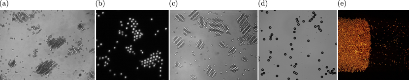
Figure 9: Experiments on the collective dynamics of spherical active colloids. (a) Phase separation of a suspension of active Janus particles activated by locally demixing a critical binary fluid [12] (adapted with permission from Ref. [12]; copyright (2013) American Physical Society). (b) Formation of dynamic clusters of self-phoretic active colloids, which interact via chemotaxis [9] (courtesy of Cécile Cottin-Bizonne). (c) Formation of living crystals by light-activated colloidal surfers consisting of hematide cube attached to a polymer sphere [10] (courtesy of Jérémie Palacci). (d) Collective motion of a monolayer of active emulsion droplets [8] (courtesy of Shashi Thutupalli). (e) Formation of a band of colloidal Quincke rollers in a racetrack geometry due to hydrodynamic and electrostatic interactions [11] (courtesy of Denis Bartolo).

4.1.2 Dynamic clustering and phase separation

Passive hard-sphere colloidal systems phase-separate at relatively large densities and in a narrow density region into a fluid and crystalline phase favored by an increase in entropy [284]. However, if one turns on activity in active particles, phase-separation can already occur at lower densities. This so-called motility-induced phase separation was first discussed in the context of run-and-tumble bacteria [175] but seems to be generic for active particles, which slow down in the presence of other particles [147, 148, 285, 36]. Typically, they phase-separate into a gaslike and a fluid-/solidlike state at sufficiently high density and swimming velocity. This happens even in the absence of any aligning mechanism [147, 148].

Simple model systems to experimentally study the influence of activity on the phase behavior of self-propelled particles are active colloidal suspensions confined to a monolayer, which is either sandwiched between two bounding plates [8, 12] or sedimented on a substrate [9, 10, 11]. These quasi-two-dimensional systems allow a relatively easy tracking of particle positions and thereby the monitoring of particle dynamics.

Probably the most simple experimental system showing motility-induced phase separation was introduced by Buttinoni et al. using light-activated spherical Janus particles that swim in a binary fluid close to the critical demixing transition (see also section 2.2.1). Tuning the laser intensity, the swimming speed – and therfore the Péclet number – can be adjusted. Since phoretic and electrostatic interactions between colloids seem to be negligible in these experiments, the Janus particles serve as a simple experimental model for active hard spheres swimming in a low Reynolds number fluid. At sufficiently low Péclet number and areal density, the particles do not form clusters but rather behave as an active gas. However, for higher particle density and swimming speed, densely packed clusters emerge, which coexist with a gas of active particles (see figure 9(a)). Increasing the Péclet number, the size of these clusters grow, as predicted earlier by simulations and theory (see chapter 4.2 and 4.3).

Very dynamic particle clusters form in the experiments of Theurkauff et al. with self-phoretic spherical colloids half-coated with platinum, which become active when adding $\textrm{H}_{2}\textrm{O}_{2}$ [9] [see figure 9(b)]. Effective particle interactions exist, both attractive and repulsive, which in combination can produce pronounced dynamic clustering already at very low area fractions of a few percent [9, 190, 192]. These effective forces arise from diffusiophoresis, which the colloids experience in non-uniform chemical fields produced by their neighbors while consuming $\textrm{H}_{2}\textrm{O}_{2}$ (see also chapter 3.3). Therefore, such artificial systems can mimic chemotactic processes found in biological systems. Aggregation of chemotactic active colloids was also reported in further experiments [182, 184, 187, 10, 286].

Most recently, the sedimentation profile of interacting self-phoretic colloids under gravity was studied in detail [177]. Here, far away from the bottom surface the density of swimmers is very small and shows an exponential decay as described in section 3.2. Closer to the bottom clusters are formed due to phoretic interactions at semi-dilute particle suspensions. The cluster formation could be mapped to an adhesion process of a corresponding equilibrium system.

Palacci et al. investigated the collective motion of colloidal surfers (see section 2.3) on a substrate. Here again, the combination of self-propulsion and steric and chemical interactions triggers the formation of clusters [10], which show a well-defined crystalline structure [see figure 9(c)]. These living crystals are highly dynamic; they form, rearragange, and break up quickly.

All of these systems show the emergence of positional order through the formation of clusters, but no significant orientational order in the swimming direction has been reported. Nevertheless, even for spherical active particles polar order can emerge in the presence of hydrodynamic, electrostatic, or other interactions between nearby particles. They lead to a local alignment of swimmer orientations, as we report in the following section.

4.1.3 Swarming and polarization

Local mechanisms for aligning active particles give rise to new collective phenomena. We summarize them here.

Quite surprisingly, even for spherical active colloids, where an aligning mechanism is not obvious, polar order was reported in a dense suspension of swarming active emulsion droplets [8] [see figure 9(d)]. The observed large-scale structures and swirls show some behavior reminiscent of biological swarms [1]. Hydrodynamic interactions between active droplets, due to the flow fields they create, are expected to play an important role. However, their details are not fully clear. Marangoni flow at the droplet surfaces cause hydrodynamic flow fields in the bulk fluid (see section 2.2.2), but this Marangoni flow might be modified by the presence of other active droplets. It remains to be investigated how this effects the collective dynamics. Noteworthy, the system reported in Ref. [8] is strongly confined in the plane by a curved petri dish, which seems to be important for observing the swarming dynamics. Similar behavior was noted for vibrated granular matter [287, 288, 289]. Finally, swimming liquid crystal droplets form crystalline rafts that float above the substrate [56].

Bricard et al. studied the collective motion of Quincke rollers (see section 2.3) in a racetrack geometry [11]. Here, both electrostatic and hydrodynamic interactions between the rollers determine their collective motion. For constant strength of the applied electric field, the collective motion can be tuned by modifying the area fraction of the particles. While at sufficiently low densities the particles form an apolar active gas, at a critical density propagating polar bands emerge [see figure 9(e)]. At even higher densities a polar liquid is stabilized, where all particles move in the same direction. Interestingly, when the confining geometry is changed to a square or to a circular disc, a single macroscopic vortex forms [11, 290]. Similar vortices occur in circularly confined bacterial suspensions [291, 131].

In a very recent work, Nishiguchi and Sano observed active turbulence in a monolayer of swimming spherical colloids [13]. Here, the Janus colloids sediment on a substrate and start to swim when an AC electric field is applied. While both hydrodynamic and electrostatic interactions seem to play a role for generating turbulence, the detailed mechanisms are not well understood yet. Noteworthy, up to now active turbulent states have only been observed for non-spherical active particles.

4.2 Modeling and analysing the collective motion of active colloidal suspensions

4.2.1 Active Brownian particles

The most basic realization for studying interacting active colloids in theory and simulations are active Brownian particles (ABPs) (see also section 2.4). The equations of motion for a single, free ABP are given in equations (21) and (22), and the solution is a persistent random walk (see section 3.1).

The dynamics of interacting ABPs can be implemented in different ways using Brownian dynamics or even kinetic Monte Carlo simulations [292]. To account for the fact that particles cannot interpenetrate each other due to steric repulsion, hard or soft potentials between the ABPs are typically used. For example, the Weeks-Chandeler-Anderson (WCA) potential $V(r)$ is employed frequently to model soft-core or (almost) hard-core repulsion between two particles. It is a Lennard-Jones potential acting between spherical particles of radius $R$ and cut off at distance $d^{\ast}$, where the Lennard-Jones Potential has its minimum [293],

$$V(r)=\left\{\begin{array}[]{rl}4\epsilon\left[{\left(\frac{\sigma}{r}\right)}^{12}-{\left(\frac{\sigma}{r}\right)}^{6}\right]+\epsilon,&\textnormal{for }r<d^{\ast}\\ 0,&\textnormal{for }r\geq d^{\ast}.\end{array}\right.$$ (47)

Here, $d^{\ast}=2^{1/6}\sigma$, $\epsilon$ is the potential strength, and $\sigma=2R/2^{1/6}$ is chosen such that the interaction force $\mathbf{F}=-\boldsymbol{\nabla}V$ becomes non-zero at $d^{\ast}<2R$, i.e., when two ABPs overlap. A simple alternative to implement hard-core interaction is the following [10, 190]: whenever particles overlap during a simulation, one separates them along the line connecting their centers.

Then, in a system consisting of $N$ active particles the equation of motion for the $i$-th particle reads

$$\dot{\mathbf{r}}^{(i)}=v_{0}\mathbf{e}^{(i)}+\mu\sum_{j\neq i}\mathbf{F}^{(ij)}+\sqrt{2D}\boldsymbol{\xi}\,,$$ (48)

where the index $j$ runs over all other $N-1$ particles, $\mathbf{F}^{(ij)}$ is the interaction force from particle $j$ on $i$, and $\mu=(6\pi\eta R)^{-1}$ is the mobility coefficient of the ABP. Together with the equation for the stochastic reorientation of the particle orientations $\mathbf{e}^{(i)}$ [see equation (22)] equation (48) is solved, e.g., by Brownian dynamics simulations. Additional attractive and/or repulsive interactions may be included [294, 150].

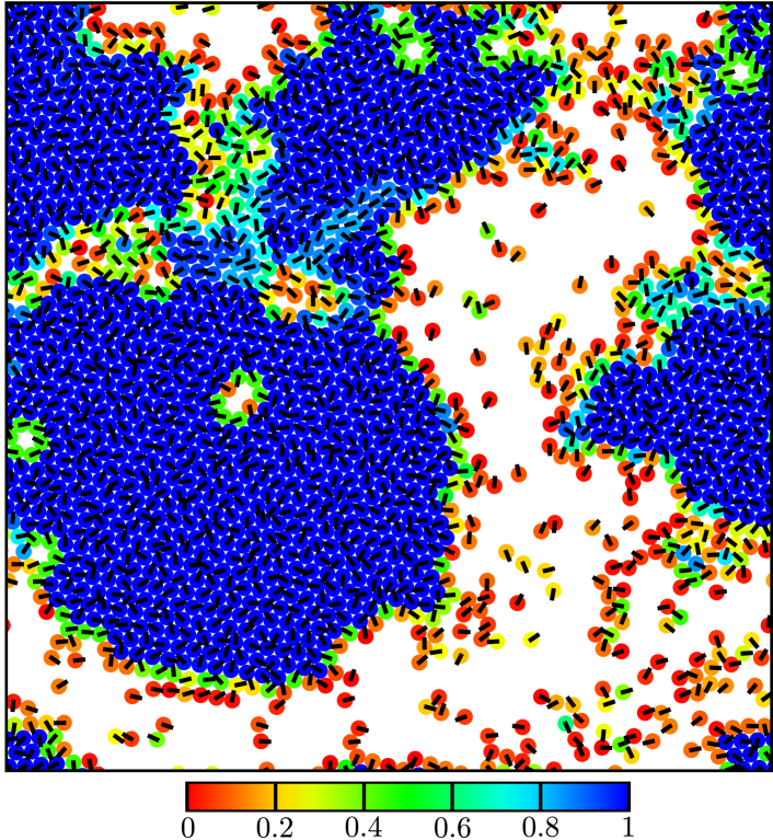
Figure 10: Snapshot of a phase-separated suspension of active Brownian disks (area fraction $\phi=0.64$, Péclet number $\textrm{Pe}=360$). The (almost) hard-core repulsion was implemented by using a WCA potential [equation (47)] with $\epsilon=1000$. The color indicates the local 6-fold bond-orientational order measured by $|q_{6}|^{2}$ from equation (57).

While elongated ABPs tend to align with neighbors after steric collisions [156, 159, 157], active Brownian spheres and disks lack any intrinsic aligning mechanism. Nevertheless, different mechanisms such as aligning, phoretic, or hydrodynamic interactions alter the particle orientations $\mathbf{e}^{(i)}$ and can be included into equation (22) for the orientation vector (see, for example, [295, 296, 10, 190, 297, 298]).

In theory and simulations, the simplest system for studying collective motion of active Brownian particles consists of active Brownian disks, which interact only via hard-core repulsion in two dimensions (2D). This minimal model has frequently been used to investigate the collective dynamics of active particles [147, 145, 148, 12, 294, 271, 272, 154, 155, 152, 299, 300, 301, 302, 303]. Bialké et al. [145], Fily et al. [147], and Redner et al. [148] were the first to explore dynamic structure formation within this model. The two relevant parameters in the system are the areal density $\phi$ and the Péclet number Pe. The latter is linear in the persistence number $\textrm{Pe}_{r}$ for pure thermal noise [see equation (29)]. While at low densities the ABPs form an active gas, they start to phase-separate into a gaslike and a crystalline phase at $\phi\gtrsim 0.3$ and sufficiently large Pe [147, 148, 12, 294, 271, 272, 154, 155, 37]. Figure 10 shows a typical snapshot of the phase-separated state for $\phi=0.64$ and $\textrm{Pe}=330$. The crystalline structure is not perfect but also contains defects. For sufficiently small Péclet numbers the dense cluser phase is rather liquidlike [145, 148].

In three dimensions (3D) the system also phase-separates. However, the cluster phase does not have crystalline order but is rather fluidlike and the local density can reach the random-close-packing limit [304]. Furthermore, the coarsening dynamics of the clusters clearly differ in 2D and 3D. While in 3D the mean domain size grows as $\sim t^{1/3}$ in time [155], similar to equilibrium coarsening dynamics, a cluster coarsens more slowly in 2D according to $\sim t^{0.28}$ [294, 271, 155].

We note that the minimal model can be extended in several ways leading to new emergent collective behavior. For example, introducing polydispersity in the ABPs, results in active glassy behavior [305, 149, 292, 151, 306, 307]. Additional attractive interparticle forces lead to gel-like structures [294] or very dynamic crystalline clusters at low densities [10, 150, 190]. The collective motion of self-propelled Brownian rods was studied extensively [156, 159, 157, 158, 288, 308, 309, 310, 311, 161]. Due to the local alignment of the rods, one observes the formation of dynamic swarming clusters [156], moving bands [309], and even turbulent states [161]. Finally, the self-assembly of active particles with more complex shapes was investigated [166, 312].

To summarize, the simple model of ABPs is able to qualitativly reproduce important aspects of the observed emergent behavior in active colloids such as motility-induced phase separation (see section 4.1.2) by only accounting for self-propulsion and steric hindrance. However, it neglects the effect of flow fields generated by active colloids and does not include phoretic interactions, which we will discuss in sections 4.2.2 and 4.2.5.

4.2.2 Microswimmers with hydrodynamic interactions

As we have discussd in section 2, active colloids moving in a Newtonian fluid create a flow field around themselves. In the following, we discuss how these flow fields determine the collective dynamics of microswimmers.

Hydrodynamic interactions between active colloids

We shortly introduce here the basic principles of hydrodynamic interactions between microswimmers (see also Refs. [122, 313, 15, 16, 5, 297, 19]). Active colloids at positions $\mathbf{r}_{i}$ and swimming in bulk with velocities $\mathbf{U}_{i}=v_{0}\mathbf{e}_{i}$ create undisturbed flow fields $\mathbf{v}_{i}(\mathbf{r};\mathbf{r}_{i},\mathbf{e}_{i})$ around themselves, when they are far apart from each other. The flow fields depend on the swimmer type, as discussed in section 2. In leading order of hydrodynamic interactions, each microswimmer is advected by the undisturbed flow fields from their neighbors and the colloidal velocity becomes $\mathbf{U}_{i}^{\prime}=\mathbf{U}_{i}+\mathbf{U}_{i}^{\mathrm{HI}}(\{\mathbf{r}_{j},\mathbf{e}_{j}\})$ with $\mathbf{U}_{i}^{\mathrm{HI}}=\sum_{j\neq i}\mathbf{v}_{j}(\mathbf{r}_{i};\mathbf{r}_{j},\mathbf{e}_{j})$. In addition, the vorticities of the undisturbed flow fields add up to determine the angular velocities $\boldsymbol{\Omega}_{i}^{\prime}=\boldsymbol{\Omega}_{i}^{\mathrm{HI}}(\{\mathbf{r}_{j},\mathbf{e}_{j}\})$ in leading order. When particles come closer together, the undisturbed flow fields do not satisfy the no-slip boundary condition at the surfaces of neighboring particles. They have to be modified and thereby the hydrodynamic contributions, $\mathbf{U}_{i}^{\mathrm{HI}}(\{\mathbf{r}_{j},\mathbf{e}_{j}\})$ and $\boldsymbol{\Omega}_{i}^{\mathrm{HI}}(\{\mathbf{r}_{j},\mathbf{e}_{j}\})$, to the colloidal velocities change.

Still in the dilute limit, where the distances between the swimmers are much larger than their radii, one can improve on the far-field hydrodynamic interactions using Faxén’s law [59]. For example, for spherical particles of radius $R$ the hydrodynamic contributions $\mathbf{U}_{i}^{\mathrm{HI}}$ and $\boldsymbol{\Omega}_{i}^{\mathrm{HI}}$ to the colloidal velocities read

$$\mathbf{U}_{i}^{\mathrm{HI}} =\sum_{j\neq i}\left(1+\frac{R^{2}}{6}\nabla_{i}^{2}\right)\mathbf{v}_{j}(\mathbf{r}_{i};\mathbf{r}_{j},\mathbf{e}_{j}),$$ (49)

$$\boldsymbol{\Omega}_{i}^{\mathrm{HI}} =\frac{1}{2}\boldsymbol{\nabla}_{i}\times\sum_{j\neq i}\mathbf{v}_{j}(\mathbf{r}_{i};\mathbf{r}_{j},\mathbf{e}_{j})\,$$ (50)

where $\mathbf{v}_{j}(\mathbf{r}_{i};\mathbf{r}_{j},\mathbf{e}_{j})$ is again the undisturbed flow field created by swimmer $j$ and evaluated at the position $\mathbf{r}_{i}$ of swimmer $i$. Similar expressions hold for ellipsoidal particles [58, 61].

In more dense suspensions of active colloids the approximation of far-field hydrodynamics [equations (49) and (50)] is not valid any more. In contrast, $\mathbf{U}_{i}^{\mathrm{HI}}$ and $\boldsymbol{\Omega}_{i}^{\mathrm{HI}}$ are mainly determined by near-field hydrodynamic interactions. Their calculation is much more complicated and strongly depends on the specific swimmer model. Hence, they usually have to be determined via hydrodynamic simulations, which capture the hydrodynamic near fields correctly. For squirmers lubrication theory can be applied to calculate $\mathbf{U}_{i}^{\mathrm{HI}}$ and $\boldsymbol{\Omega}_{i}^{\mathrm{HI}}$, but it only holds for interparticle distances $d\ll R$ [122].

Collective motion of squirmers

The squirmer model introduced in section 2.2.3 is a simple model to study how hydrodynamic interactions influence the collective motion of active colloids. Ishikawa and Pedley were the first to use the boundary element method and Stokesian dynamics simulations for investigating the collective motion of squirmers in bulk fluids [314, 315, 316, 317, 318, 319, 320, 321]. Typically, in a suspension of squirmers the reorientation rates $\boldsymbol{\Omega}_{i}^{\mathrm{HI}}$ chaotically evolve in time and hydrodynamic interactions thus modify rotational diffusion and an increased effective diffusion constant $D_{r}^{\mathrm{HI}}$ results [314, 322]. For squirmer pullers polar order can emerge[317], which was also quantified further in Refs. [323, 324, 325]. This is in contrast to hydrodynamic simulations of self-propelled rods, which show local polar order for generic pushers but not for pullers (see the last paragraph of this section). The reason for the different behavior of squirmer and active rod suspensions might be due to different types of near-field hydrodynamic interactions as dicussed in section 3.5.

Noteworthy, in large suspensions of squirmer pullers temporal density variations emerge, where a large cluster periodically forms and breaks apart [324]. The time correlation function of these density fluctuations show oscillatory behavior with a well-defined frequency. Recently, also the dynamics of many squirmers confined between two hard walls has been studied [326, 327, 154, 245, 328]. For a separation distance much larger than the swimmer size, again a huge dynamically evolving cluster emerges. It travels between the walls and has been interpreted as a propagating sound wave [328].

Recent investigations studied the collective motion of squirmers moving either in 2D [329, 330, 331] or in quasi-2D [154] in order to reveal the influence of hydrodynamic interactions on the dynamics of active colloidal suspensions. The quasi-2D geometry constrained the squirmers to a monolayer similar to experiments in Ref. [12] (see section 4.1). 2D simulations showed that long-range hydrodynamic interactions result in strong reorientation rates $\boldsymbol{\Omega}_{i}^{\mathrm{HI}}$ that are sufficient to entirely suppress motility-induced phase separation of squirmers [330]. Simpler non-squirming swimmers simulated with the lattice-Boltzmann method in 2D [332, 333] and with Stokesian dynamics in a monolayer in 3D [334] showed some clustering.

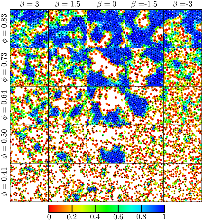
Figure 11: Collective motion of squirmers in a quasi-2D geometry depending on the area fraction $\phi$ and squirmer parameter $\beta$. The color indicates the local 6-fold bond-orientational order measured by $|q_{6}|^{2}$ from equation (57). (Adapted from Ref. [154]; copyright (2014) American Physical Society.)

We performed three-dimensional MPCD simulations of squirmers and strongly confined them between two parallel plates, such that they could only move in a monolayer (quasi-2D geometry) [154]. The simulations were based on Refs. [124, 170, 203], where single squirmers were implemented with MPCD. Our results showed that the phase behavior of squirmers strongly depends on the swimmer type, characterized by the squirmer parameter $\beta$, and on areal density $\phi$ (see figure 11). While neutral squirmers ($\beta=0$) and weak pushers ($\beta<0$) phase-separate at a sufficiently high density, pullers ($\beta>0$) only form small and short-lived clusters. Strong pushers do not cluster at all and only develop one crystalline region at high areal densities. They tend to point with their swimming directions perpendicular to the bounding walls, which significantly reduces their in-plane persistent motion so that clustering does not occur. Pullers are more oriented parallel to the walls. But their rotational diffusivity is strongly enhanced so that the persistent motion is again too small to exhibit phase separation. In contrast, neutral squirmers and weak pushers also swim parallel to the walls and their hydrodynamic rotational diffusion $D_{r}^{\mathrm{HI}}$ is sufficiently small to allow stable clusters to form and hence they phase-separate. We do not observe polar order in any of the studied systems. This could be due to the presence of the walls or thermal noise, which was absent in all the other simulations on the collective dynamics of squirmers. We currently perform large-scale simulations, which confirm all these findings and clearly demonstrate the first-order phase transition associated with phase separation.

Collective motion of elongated microswimmers and actively spinning particles

At present experiments have focussed on the emergent behavior of spherical active colloids, as described in sections 4.1.2 and 4.1.3. Nevertheless, we expect that in the near future novel experiments on the collective motion of self-propelled rod-shaped colloids will be performed.

Aditi Simha and Ramaswamy were the first to study the role of long-range hydrodynamic interactions in the collective motion of swimming force dipoles with polar or nematic order using continuum field theory [335]. The collective motion of hydrodynamically interacting active dumbbells, which are modeled as pairs of point forces, was addressed in Refs. [336, 337] and later in Ref. [338] using dissipative particle dynamics. More refined, explict simulations of hydrodynamically interacting self-propelled rods were performed by Saintillan and Shelley [126, 129], Lushi et al. [130, 131], and Krishnamurthy and Subramanian [339] based on slender-body theory. Unlike squirmer suspensions, pusher rods and dumbbells show local polar (as well as nematic) order and form large-scale vortices, in qualitative agreement with experiments with pusher-type bacteria [260, 162]. Typically, in these simulations only approximate flow fields based on far-field hydrodynamics were implemented. A recent simulation study with active dumbbells improved the resolution of hydrodynamic interactions between the swimmers using the method of fluid particle dynamics [340]. Motility-induced phase separation was observed, and it was shown that hydrodynamic interactions enhanced cluster formation. Yang et al. studied the hydrodynamics of collectively swimming flagella and observed the formation of dynamic jet-like clusters of synchronously beating flagella [308]. Finally, recent simulations investigated the collective motion of actively rotating disks, which tend to form crystalline structures [341, 342].

4.2.3 External fields: gravity and traps

As discussed in section 3.2, a suspension of non-interacting active colloids under gravity shows an exponential sedimentation profile [66] and develops polar order against gravity [173]. The presence of hydrodynamic interactions in a dilute suspension of sedimenting run-and-tumble swimmers does not significantly modify such a sedimentation profile [249]. However, when active Brownian particles are strongly bottom-heavy, they collect in a layer while swimming against the upper boundary of a confining cell. This layer is unstable, when hydrodynamic interactions are included, and the particles move downwards in plumes similar to observations made in bioconvection [343, 200].

A similar instability occurs for run-and tumble swimmers [249] and active Brownian particles of radius $R$ [297], when they move in a harmonic trap potential while interacting hydrodynamically. The microswimmers form a macroscopic pump state that breaks the rotational symmetry of the trap. The radial force $\mathbf{F}=-k\mathbf{r}$ $(k>0)$ confines the particles to a spherical shell of radius $r_{\mathrm{hor}}=R\mathrm{Pe}/\alpha$, where $\alpha=kR^{2}/k_{B}T$ is the trapping Péclet number [297]. When started with random positions and orientations, the active particles first accumulate at the horizon at radial distance $r_{\mathrm{hor}}$, where they point radially outwards [249, 297]. Due to the externally applied trapping force, each particle initiates the flow field of a stokeslet, in leading order. However, a uniform distribution of stokeslets on the horizon sphere, all pointing radially outward, is not stable against small perturbations. In particular, particles’ swimming directions are rotated by nearby stokeslets. The particles move towards each other creating denser regions, which are advected towards the center. At sufficiently large swimmer density the active particles align in their own flow field and thereby generate a macroscopically ordered state [see figure 12(a)], quantified by the global polar order parameter $\mathcal{P}$ (see also section 4.3.4). The coarse-grained flow field, created by the swimmers, has the form of a regularised stokeslet and pumps fluid along the polar axis to the center of the trap. The pump formation does not occur, if the Péclet number, the trapping strength, or the density is too small, as shown in figure 12(b).

Interestingly, the form of the distribution $\Phi(\theta)$ of orientation angles $\theta$ measured against the pump axis can be calculated analytically from the corresponding Smoluchowski equation. One obtains $\Phi(\theta)\sim\exp(A\cos\theta)$, reminiscent of dipoles aligning in a field $A$, which is produced by the swimmers themselves. In simulations we find $A\sim(\mathrm{Pe}\mathcal{P})^{\gamma}$, with $\gamma\approx 1$ for low densities and decreasing for higher densities. Thus, the mean flow field created by all the swimmers and the associated polarization $\mathcal{P}$ play the same respective role as the mean magnetic field and the magnetization in Weiss’ theory of ferromagnetism [297].

In Ref. [344] the collective behavior of purely repulsive active particles in two-dimensional traps was mapped on a system of passive particles with modified trapping potential and then formulated as a dynamical density functional theory [344]. In very good agreement with the numerical solution of the corresponding Langevin equations, one could show that the radial distribution in the trap including packing effects strongly depends on the Péclet number.

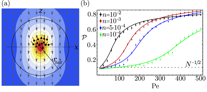
Figure 12: Pump formation of hydrodynamically interacting active particles (a) The formation of a macroscopic pump induces a regularised Stokeslet flow. (b) Global polar order parameter $\mathcal{P}$ versus Péclet number $\mathrm{Pe}$ for different volume fractions (adapted from Ref. [297]; copyright (2014) American Physical Society).

4.2.4 External flow and rheology

We have discussed the response of a single microswimmer to an externally applied flow field $\mathbf{u}$ in section 3.4. In turn, a suspension of microswimmers is able to modify $\mathbf{u}$ and the rheological properties of the fluid.

In pure Newtonian fluids the shear stress tensor $\boldsymbol{\uptau}$ is linear to the strain rate tensor, $\boldsymbol{\uptau}=\eta_{0}[\boldsymbol{\nabla}\otimes\mathbf{u}+(\boldsymbol{\nabla}\otimes\mathbf{u})^{t}]$, where $\eta_{0}$ is the shear viscosity. Adding a dilute suspension of passive colloids with volume fraction $\phi\ll 1$ is known to increase the effective viscosity $\eta$. In leading order in $\phi$ the increase is linear, $\eta=\eta_{0}(1+\frac{5}{2}\phi)$, as calculated by Einstein [345, 346]. In contrast, adding a suspension of swimming bacteria [347, 348, 349] or algae [350, 351] to water can lead to both an increase and a decrease of the viscosity; an effect which was first predicted in Ref. [352]. Strikingly, at high shear rates $\eta$ approaches zero for swimming E. coli suspensions [349], which thus becomes a superfluid. This was also predicted before for sheared active gels [353].

While up to date no experimental studies exist that measure the effective viscosity $\eta$ of active colloidal suspensions, numerical simulations were performed using the squirmer model. The rheological properties of squirmer suspensions with hydrodynamic interactions were simulated using Stokesian dynamics [314] and lattice Boltzmann simulations [327]. In Ref. [314] a semi-dilute suspension of squirmers in unbounded shear flow show almost the same, but slightly reduced, apparent viscosity as for a semi-dilute passive colloidal suspension. In wall bounded shear flow, as studied in Ref. [327], the viscosity of squimer suspensions depends strongly on the applied shear rate $\dot{\gamma}$ and on the swimmer type. While for strong $\dot{\gamma}$ the viscosity of all squirmer suspensions is comparable to the effective viscosity of passive suspensions, it can be strongly decreased or increased at lower $\dot{\gamma}$. Namely, for all squirmer suspensions with sufficiently small $|\beta|\lesssim 20$ the effective viscosity is increased ($\eta/\eta_{0}>1$), but for apolar pushers ($\beta\rightarrow-\infty$) and apolar pullers ($\beta\rightarrow\infty$) the effective viscosity is strongly decreased ($\eta/\eta_{0}<0$) and almost vanishes for very small $\dot{\gamma}$.

4.2.5 Chemotactic active colloids

As discussed in section 3.3.1, an active colloid that experiences a nonuniform background concentration field $X(\mathbf{r})$ moves with an additional phoretic velocity $\mathbf{U}_{C}$ and angular velocity $\boldsymbol{\Omega}_{C}$, which both are linear in the local field gradient $\boldsymbol{\nabla}X(\mathbf{r})$. Self-phoretic colloids act as sinks and sources in a chemical field and respond to local field gradients created by neighboring particles. This introduces an effective interaction, which can either be attractive or repulsive. In particular, active colloids can orient parallel or against a field gradient and thereby either swim towards or away from other particles.

The collective behavior of chemotactic active particles has been studied numerically with particle-based models using Langevin dynamics simulations [354, 10, 190, 192], and theoretically by continuum models [181, 190, 193]. Depending on whether the active colloids are chemoattractive or chemorepulsive, or whether they tend to rotate towards or against a chemical gradient, qualitatively different collective behavior emerges [354, 10, 181, 190, 192, 193].

To capture the basic effects, we follow Ref. [190] and include diffusiophoretic attraction/repulsion and reorientation into equations (21) and (22). Then the equations of motion for $N$ interacting particles ($i=1,\dots,N$) read [190, 192]

$$\dot{\mathbf{r}}_{i} =v_{0}\mathbf{e}_{i}-\zeta_{\mathrm{tr}}\boldsymbol{\nabla}c(\mathbf{r}_{i})+\sqrt{2D}\boldsymbol{\xi}$$ (51)

$$\dot{\mathbf{e}}_{i} =-\zeta_{\mathrm{rot}}(\mathbf{1}-\mathbf{e}_{i}\otimes\mathbf{e}_{i})\boldsymbol{\nabla}c(\mathbf{r}_{i})+\sqrt{2D_{r}}\boldsymbol{\xi}_{r}\times\mathbf{e}_{i}\,,$$ (52)

where $\zeta_{\mathrm{tr}}$ is the translational diffusiophoretic parameter, which quantifies chemoattraction ($\zeta_{\mathrm{tr}}>0$) and chemorepulsion ($\zeta_{\mathrm{tr}}<0$), and $\zeta_{\mathrm{rot}}$ is the rotational diffusiophoretic parameter, which describes reorientation along ($\zeta_{\mathrm{rot}}>0$) and against ($\zeta_{\mathrm{rot}}<0$) chemical gradients. Here, the chemical field $c(\mathbf{r})$ created by the swimmers is assumed to be a stationary sink, which moves around with the particles. In leading order it decays linearly with the distance from the swimmer [47] but is screened due to the presence of other particles [10, 190]. Dipolar contributions and higher multipoles are neglected. We discuss here the two-dimensional motion of relatively dilute systems (area fraction $5\%$) similar to experiments [9, 10].

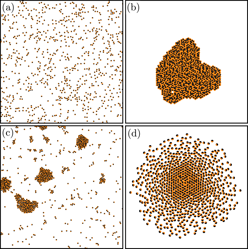
Figure 13: Collective motion of chemotactic active colloids at $5\%$ area fraction depending on the diffusiophoretic parameters $\zeta_{\mathrm{tr}}$ and $\zeta_{\mathrm{rot}}$. (a) Gaslike state for small $\zeta_{\mathrm{tr}}$ and $\zeta_{\mathrm{rot}}$. (b) Collapsed single-cluster state for sufficiently large $\zeta_{\mathrm{tr}}$. (c) Dynamic clustering for $\zeta_{\mathrm{rot}}<0$ and sufficiently large $\zeta_{\mathrm{tr}}>0$. (d) Core-corona state for chemorepulsion ($\zeta_{\mathrm{tr}}<0$). [(a)-(c) adapted from Ref. [190]; copyright (2014) American Physical Society. (d) adapted from Ref. [192]; with kind permission of The European Physical Journal (EPJ).]

First, for sufficiently small $\zeta_{\mathrm{tr}}$ and $\zeta_{\mathrm{rot}}$ the particles are in a gaslike state, where they hardly cluster [see figure 13(a)], similar to active Brownian disks which interact purely due to steric hindrance [147, 148]. Second, for sufficiently strong attraction all the particles end up in a collapsed state and form a single stable cluster [354, 190, 181] reminiscent of the chemotactic collapse obtained from the Keller-Segel model [355] [see figure 13(b)]. Third, for $\zeta_{\mathrm{rot}}<0$ and sufficiently large $\zeta_{\mathrm{tr}}>0$ dynamic clustering is observed [see figure 13(c)] in good agreement with experiments [9, 10]. Dynamic clusters form since chemoattraction is balanced by the reorientation of the swimmers such that they try to swim away from each other. The cluster-size distribution (see also section 4.3.2) follows a power-law decay. Fourth, in the opposite case, for chemorepulsion ($\zeta_{\mathrm{tr}}<0$) but alignment against the chemical gradient ($\zeta_{\mathrm{tr}}>0$) an oscillating state can emerge, where all particles periodically collapse and dissolve [192]. Further decreasing $\zeta_{\mathrm{tr}}$, the particles ultimately arrange in a stable core-corona state as shown in figure 13(d), which also occurs when screening is turned off. Oscillating states reminiscent of plasma oscillations and aster formation were also observed in a continuum model [181]. Different scenarios for pattern formation in chemorepulsive active colloids have recently been explored in Ref. [193].

The collective behavior of a dilute suspension of light-heated active colloids interacting by thermoattraction and thermorepulsion was analyzed in Ref. [356]. While thermorepulsive colloids show a depletion zone in the center of a confining region, thermoattractive colloids aggregate in the center and collapse at sufficiently high density [356]. Using Brownian dynamics simulations, the formation of a dense cometlike swarm, which consists of interacting thermally active colloids moving towards an external light source, was reported [357]. Finally, Ref. [191] discusses the orientation of thermally active Janus particles in a temperature gradient, as well as the effect of Péclet number on aggregation and dispersion of the particles.

The collective motion or pattern formation of active particles on the liquid-air interface of a thin liquid film was studied in Ref. [358], while passive but chemically active particles at the interface were treated in Ref. [359]. A 2D continuum approach to couple chemical signaling and flow fields created by pushers and pullers was used in [360].

A first work by Thakur and Kapral includes full hydrodynamic and phoretic interactions, which is computationally very expensive [112]. They studied the collective dynamics of up to 10 dimer motors in a quasi-2D geometry in the presence of thermal noise and observed dynamic cluster formation, which is mainly triggered by phoretic interactions but altered by hydrodynamic interactions [112].

4.2.6 Mixtures of active and passive colloids

Stenhammar et al. investigated the structure and dynamics of a monodisperse mixture of active and passive Brownian disks for a broad range of Péclet numbers Pe, total area fractions $\phi_{0}$, and fraction of active particles $0\leq x_{A}\leq 1$ [361]. They observed phase separation induced by the active particles. However, in contrast to motility-induced phase separation of purely active Brownian disks ($x_{A}=1$), cluster formation, cluster dynamics, and cluster break-up are much more dynamic for active-passive particle mixtures ($x_{A}<1$). At sufficiently high Pe phase separation is already possible for a relatively low amount of active particles ($x_{A}>0.15$). In the phase-separated state the active particles are mainly concentrated at the border of the clusters. This has recently been confirmed in experiments already with a very small amount ($x_{A}<3\%$) of active colloids [253]. In contrast, above the threshold density for the crystallization of passive colloids, active particles accumulate at grain boundaries. When passing through crystalline domains, active particles are able to melt them locally and create defects along their trajectory [253]. Finally, by performing event-driven Brownian dynamics simulations, Ni et al. [362] realized that a small amount of active particles helps to crystallize passive polydisperse glassy hard spheres in three dimensions.

Various types of segregation in a mixture of passive and self-propelled hard rods moving in 2D were observed by McCandlish et al. [311], i.e. swarming, coherent clustering, and transient lane formation. In dissipative particle dynamics simulations a mixture of passive and active particles showed the emergence of turbulence, polar order, and vortical flows [363].

4.3 Physical concepts of active suspensions

In sections 4.1 and 4.2 we have reviewed emergent behavior of collectively moving active colloids. In the following we will present some important concepts and measures to capture the structure and dynamics of interacting active particles more quantitatively.

4.3.1 Motility-induced phase separation

Motility-induced phase separation of active particles can mainly be understood as a self-trapping mechanism: When active particles collide, they slow down due to steric hindrance and a cluster can form for sufficiently high persistence number [285, 12, 36].

In theory, the separation of purely repulsive active Brownian particles into a liquidlike and a gaslike phase has recently been investigated by mapping the system to an equilibrium system, for which an effective free energy functional was constructed [175, 285, 271, 272, 301, 364, 365]. Here, the velocities of the particles in the presence of neighbors are typically approximated by a function $v(\rho)$ which decays almost linearly with density $\rho$ [147, 148, 271, 272, 155],

$$v(\rho)=v_{0}\left(1-\frac{\rho}{\rho{{}^{\ast}}}\right)\,,$$ (53)

where $\rho^{\ast}\approx\rho_{\mathrm{rcp}}$ is the density close to random close packing [36]. In the limit of large Péclet numbers, phase coexistence occurs when the following relation holds [175, 36],

$$\frac{dv(\rho)}{d\rho}<-\frac{v(\rho)}{\rho}.$$ (54)

The coexistence of a gaslike and a liquidlike phase emerges via spinodal decomposition; similar as in equilibrium thermodynamics, two-phase coexistence with the binodal densities $\rho_{1}$ and $\rho_{2}$ arises from the tangent construction for an effective free energy functional [175, 285, 271, 272]. Interestingly, by linearizing the underlying hydrodynamic equations [272] an effective Cahn-Hilliard equation for active phase separation can be constructed [301]. Wittkowski et al. formulated a scaler $\phi^{4}$ field theory for the order parameter field $\phi(\mathbf{r},t)$ to study phase separation and its coarsening dynamics by an Active Model B [364], which violates detailed balance. This procedure has recently been extended to include hydrodynamics by coupling $\phi(\mathbf{r},t)$ to the Navier-Stokes equations (Active Model H [366]).

A kinetic approach for determining a condition for motility-induced phase separation was formulated by Redner et al. [294, 148]. The incoming flux $j_{\mathrm{in}}$ of active particles from the gas phase of density $\rho_{g}$ onto an existing cluster is compared with the outgoing flux $j_{\mathrm{out}}$ from the border of a cluster into the gas phase. While the incoming flux, $j_{\mathrm{in}}\propto\rho_{g}\mathrm{Pe}$, is proportional to particle speed and density, the outgoing flux, $j_{\mathrm{out}}\propto\mathrm{Pe}_{r}^{-1}$, depends on the inverse persistence number and thus on rotational diffusion. Note that rotational diffusion can be strongly enhanced in the presence of hydrodynamic interactions [317] and thereby reduce or suppress phase separation [154, 330]. The condition for phase separation and the fraction of particles in the cluster are determined from the steady state condition $j_{\mathrm{in}}=j_{\mathrm{out}}$ [294, 148].

Finally, we comment on how to quantify a phase-separated state obtained from experimental or simulation data of active particles. A phase-separated state consists of a high-density (liquid- or solidlike) and a low-density (gaslike) region and has, by definition, a bimodal distribution $p(\phi_{l})$ of local densities $\phi_{l}$. The local density $\phi_{l}^{(i)}$ of particle $i$ at position $\mathbf{r}_{i}$ is typically defined via the size $A_{i}$ of its corresponding Voronoi cell [367], $\phi_{l}^{(i)}=A_{0}/A_{i}$, where $A_{0}=\pi R^{2}$ in 2D or $A_{0}=4\pi R^{3}/3$ in 3D and $R$ is the particle radius.

4.3.2 Active crystals and structural properties

To characterize if active particles are in a gas-, liquid- or crystal-like phase, further structural properties are determined from the particle positions $\mathbf{r}_{i}(t)$.

Pair correlation function

The pair correlation function (or radial distribution function) $g(r)$ measures the correlations of particles at distance $r$ and was used to characterize the structure of collectively moving active colloids [317, 112, 148, 12, 324, 150, 253]. It is defined as the local density $\rho(r)$ of active particles in a spherical shell with radius $r$ around a central particle, normalized by the mean particle density $\rho_{0}$, thus $g(r)=\rho(r)/\rho_{0}$. For example, in two dimensions it can be calculated by

$$g(r)=\frac{1}{4\pi R^{2}(N-1)\phi_{0}}\left\langle\sum_{j}\sum_{i\neq j}\delta(|\mathbf{r}_{i}-\mathbf{r}_{j}|-r)\right\rangle\,,$$ (55)

where $\phi_{0}$ and $N$ are the total area fraction and number of particles, respectively. Peaks in $g(r)$ indicate favored interparticle distances. While for a dilute gas no distances are favored and $g(r)\approx 1$, $g(r)$ shows a finite number of peaks with decreasing intensity for a liquid [see figure 14(a)], and pronounced peaks for solids, where the actual peak positions indicate the structure of the solid (e.g., hexagonal).

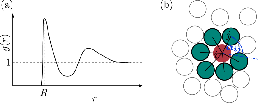
Figure 14: (a) Typical pair correlation function $g(r)$ of a liquid consisting of spherical particles of radius $R$. (b) Sketch of local structure around particle $i$ (red), and definition of the angle $\alpha_{ij}$ from equation (57) between particle $i$ and its six nearest neighbors (dark green). The arbitrarily chosen axis is shown as a dashed blue line.

Static structure factor

The Fourier transform of the pair correlation factor is the static structure factor $S(\mathbf{k})$, which identifies periodic modulations of a material with wave vector $\mathbf{k}$. It is defined as

$$S(\mathbf{k})=\frac{1}{N}\left\langle\sum_{j}\sum_{i}e^{i\mathbf{k}\cdot(\mathbf{r}_{i}-\mathbf{r}_{j})}\right\rangle\,,$$ (56)

and was used to characterize the structure of active colloidal clusters [147, 9, 11, 148, 272, 149, 155].

Bond orientational order

Clusters of active colloids moving in a monolayer often show hexagonal crystallike ordering, see sections 4.1.2 and 4.2, and figures 10, 11 and 13. The local 6-fold bond-orientational order around particle $i$ is measured by [368, 145, 294, 154]

$$|q_{6}^{(i)}|^{2}\quad\mathrm{with}\quad q_{6}^{(i)}=\frac{1}{6}\sum_{j\in N_{6}^{(i)}}e^{i6\alpha_{ij}}\,,$$ (57)

where $|q_{6}^{(i)}|^{2}\in(0,1)$, the sum goes over the six nearest neighbors of particle $i$, and the angle $\alpha_{ij}$ is measured between the distance vectors $\mathbf{r}_{i}-\mathbf{r}_{j}$ and an arbitrarily chosen axis [see figure 14(b)]. For example, for particles in a cluster with perfect hexagonal order, $|q_{6}^{(i)}|^{2}=1$, as indicated in figures 10 and 11. The mean value, $\langle|q_{6}|^{2}\rangle$, can be used as an order parameter to measure how many particles are in a dense crystal-like cluster phase [154].

Spatial correlations in the 6-fold bond-orientational order measured by $\langle q_{6}^{\ast}(\mathbf{r})q_{6}(\mathbf{r}^{\prime})\rangle$ [148] and correlations of particle $i$ with its six nearest neighbors, $\mathrm{Re}\frac{1}{6}\sum_{j\in N_{6}^{(i)}}q_{6}^{(i)}q_{6}^{\ast(j)}$, [369, 145] was used to distinguish between liquidlike, hexaticlike, and solidlike structures [145, 148]. The global bond-orientational order parameter $|\langle q_{6}\rangle|^{2}$ indicates an overall structural order in the system. Note, however, that in general $|\langle q_{6}\rangle|^{2}$ depends on the system size. Only for a perfect crystal, $|\langle q_{6}\rangle|^{2}=1$, independent of system size.

Cluster size distributions

A cluster is typically defined by a set of particles with a maximum distance $\epsilon$ between neighboring particles. One characterizes the clusters in a system of active colloids by a cluster size distribution $p(N_{c})$, where $N_{c}$ is the number of particles in the cluster [156, 9, 147, 12, 190, 151, 253]. In the gas phase $N_{c}=1$ (isolated particle) and $N_{c}=2$ (two colliding particles) mainly occur, whereas clusters with $N_{c}\gg 1$ dominate in the dense phase. In phase-separating active colloidal suspensions the size of the largest cluster in the long-time limit was used as an order parameter to study the onset of phase separation [12].

4.3.3 Giant number fluctuations

In thermal equilibrium the number of particles $N$ in a volume $V$ in a grand canonical ensemble fluctuates with standard deviation $\Delta N=\sqrt{\langle N^{2}\rangle-\langle N\rangle^{2}}\sim\sqrt{N}$ [370]. In contrast, self-propelled particle systems that are out of equilibrium often show giant number fluctuations indicated by $\Delta N\sim N^{\alpha}$ with $0.5<\alpha\leq 1$. This was predicted [335, 371, 372, 41] and first demonstrated in experiments with vibrated granular rods [287] (see also the discussion in Ref. [373]). Giant number fluctuations were also reported in dynamic clustering of active colloids [10] and in simulations of active Brownian particles [296, 147, 161]. However, electrostatic and hydrodynamic interactions suppress giant number fluctuations in dense suspensions of polarly ordered Quincke rollers [11].

4.3.4 Correlation functions and order parameters

So far, in section 4.3, we have described quantitative measures using particle positions $\mathbf{r}_{i}$. In the following, we consider particle orientations $\mathbf{e}_{i}$ and velocities $\mathbf{v}_{i}$ to characterize orientational order in the system.

Polar order

To quantify global polar order in a suspension of active colloids, the order parameter

$$P(t)=\left|\langle\mathbf{e}(t)\rangle\right|=\frac{1}{N}\left|\sum_{i}\mathbf{e}_{i}(t)\right|$$ (58)

was used in squirmer suspensions [317, 323, 324, 325] or for active particles in a harmonic trap [297]. In all these cases the particles are spherical and the aligning mechanisms have a pure hydrodynamic origin. In the long-time limit $P(t)$ typically reaches a steady state with $\mathcal{P}=\mathrm{lim}_{t\rightarrow\infty}P(t)$. For fully developed polar order $\mathcal{P}=1$. However, even an ensemble of randomly oriented particles shows a residual value for the order parameter: $\mathcal{P}\approx N^{-1/2}$ [317]. Interestingly, as reviewed in section 4.2.3 and demonstrated for collectively moving Quincke rollers, the formation of polar order at a critical density or a critical Péclet number can be mapped to the onset of ferromagnetic order treated within mean-field theory [11, 297]. In the continuum limit the polarisation becomes $\mathcal{P}=|\int_{\mathbb{S}_{2}}\Phi(\mathbf{e})\mathbf{e}dS|$ [11, 297], where $dS$ is the surface element on the unit sphere $\mathbb{S}_{2}$, and $\Phi(\mathbf{e})$ the orientational distribution function in steady state.

To measure the temporal correlations of the orientation vector $\mathbf{e}$, the autocorrelation function $C_{p}=\langle\mathbf{e}(t)\cdot\mathbf{e}(0)\rangle$ from equation (25) for a single particle is calculated and then averaged over all particles, $\overline{C}_{p}=\overline{\langle\mathbf{e}(t)\cdot\mathbf{e}(0)\rangle}$. If the decay of $\overline{C}_{p}$ is exponential, $\overline{C}_{p}=e^{-2D_{r}^{\mathrm{eff}}t}$, $D_{r}^{\mathrm{eff}}$ defines an effective rotational diffusion constant. For example, due to hydrodynamic or phoretic interactions it can have a larger value than the coefficient $D_{r}$ of an isolated swimmer [317, 112, 154]. Hence, $D_{r}^{\mathrm{eff}}$ quantifies the orientational persistence of interacting microswimmers.

Spatial correlations of particle orientations at distance $r$ and at time $t$ are described with the equal-time polar pair correlation function [126]

$$C_{e}(r,t)=\frac{\langle\sum_{i\neq j}(\mathbf{e}_{i}(t)\cdot\mathbf{e}_{j}(t)\rangle^{2})\delta(|\mathbf{r}_{i}-\mathbf{r}_{j}|-r)\rangle}{\langle\sum_{i\neq j}\delta(|\mathbf{r}_{i}-\mathbf{r}_{j}|-r)\rangle}.$$ (59)

The average is taken over all pairs of swimmers $i,j$. Note that the maximum distance $r$ in equation (59) is set by the systems size of the experiment or simulation. In experiments it is often more convenient to measure particle velocities $\mathbf{v}_{i}$ instead of their orientations $\mathbf{e}_{i}$. Then, the spatial correlation function $C_{v}(r,t)$ is defined as $C_{e}(r,t)$ in equation (59) but with orientation vectors replaced by velocities.

From the decay of the time-averaged correlation functions $C_{e}(r)=\frac{1}{T}\int_{0}^{T}C_{e}(r,t)dt$ and $C_{v}(r)=\frac{1}{T}\int_{0}^{T}C_{v}(r,t)dt$, one can determine correlation lengths $l_{c}$ for orientations and velocities in the system [260, 126, 317, 318, 337, 374, 8, 375]. Anticorrelations ($C_{e}<0$ or $C_{v}<0$) indicate the formation of vortices, for example, in turbulent bacterial suspensions [260, 376].

To characterize the mobility of collectively moving active colloids, the dynamic order parameters

$$V_{1}(t)=\left|\langle\mathbf{v}(t)\rangle\right|=\frac{1}{N}\left|\sum_{i}\mathbf{v}_{i}(t)\right|$$ (60)

and

$$V_{2}(t)=\langle\mathbf{v}(t)\cdot\mathbf{e}(t)\rangle=\frac{1}{N}\sum_{i}\mathbf{v}_{i}(t)\cdot\mathbf{e}_{i}(t)$$ (61)

were used. While $V_{1}$ simply measures the mean speed of the particles (see, e.g., [316, 330]), $V_{2}$ determines how fast they move along their intrinsic directions $\mathbf{e}_{i}$ (see, e.g., [112, 154, 330]). Possible deviations of $V_{2}$ from the swimming velocity $v_{0}$ always indicate colloidal interactions.

We note that equal-time correlations functions $C_{u}(r,t)$ and $C_{\omega}(r,t)$ are formulated for the hydrodynamic flow field $\mathbf{u}(\mathbf{r},t)$ and vorticity field $\boldsymbol{\omega}(\mathbf{r},t)=\nabla\times\mathbf{u}(\mathbf{r},t)$ created by the motion of microswimmers (see, e.g., [377]). Particularly interesting are the Fourier transforms of the time-averaged correlation functions, $\int C_{u}(r,t)dt$ and $\int C_{v}(r,t)dt$, which are used to define the energy spectrum $E(k)$ in an active fluid. It was applied to characterize active turbulence in bacterial [162] and active colloidal [13] suspensions. An order parameter for the strength of vorticity in the fluid is the so-called enstrophy, which is the spatial average of $\boldsymbol{\omega}^{2}$.

4.3.5 Mean square displacement

In order to quantify the temporal evolution of $N$ interacting active colloids by means of their trajectories $\mathbf{r}_{i}(t)$, the particle-averaged mean square displacement

$$\langle\Delta r^{2}(t)\rangle=\frac{1}{N}\sum_{i=1}^{N}|\mathbf{r}_{i}(t)-\mathbf{r}_{i}(0)|^{2}\rangle$$ (62)

is used [112, 147, 148]. Recall that for a single particle [equation (30)] the motion is ballistic ($\sim t^{2}$) at small times and diffusive ($\sim t$) at large times. Collective motion can introduce an intermediate superdiffusive regime $\sim t^{3/2}$ [112, 148] and interactions between active particles typically reduce the long-time diffusion constant extracted from equation (62) compared to free swimmers.

4.3.6 Active thermodynamics

In equilibrium thermodynamics macroscopic state variables such as temperature $T$ and pressure $p$ are well-defined quantities. The values calculated from their microscopic definitions coincide with the values obtained by introducing them as first derivates of the thermodynamic potentials. Temperature and pressure are connected via an equation of state, for example, for an ideal gas one has $pV=nRT$.

In nonequilibrium thermodynamics it is in general not possible to define state variables such as $T$ and $p$ in a meaningful way. Nevertheless, very recently quite a lot of effort has been made in formulating a thermodynamic description of active matter systems (see, e.g., the discussions in [36, 378, 379, 380, 177, 38]). For example, as already discussed in section 4.3.1, motility-induced phase separation can sometimes be addressed with an effective free energy [36] and the activity-induced collisions of the particles mapped to an effective attraction potential [303]. Another example is the controverse discussion about the concept of effective temperature in active particle systems [381, 66, 382, 383, 384, 177]. Indeed, sometimes one can assign an effective temperature to the stochastic motion of active colloids. Examples are the persistent random walk in bulk (see section 3.1) or the sedimentation profile of non-interacting active particles in a gravitational field (see section 3.2). In general, however, it is not possible to treat the stochastic dynamics of microswimmers with an effective temperature.

Active pressure

Very recently some research groups have started to work on defining pressure in active particle suspensions [299, 254, 152, 300, 378, 255, 385, 386, 380, 387, 388, 389, 390, 391, 392, 38] by using various definitions for pressure. First, one views pressure as the mechanical force, which an active particle system in a container exerts per unit area on bounding surfaces. Second, in bulk it should be the trace of the hydrodynamic stress tensor. Third, pressure can be calculated as the derivative of a free energy with respect to volume. Since, in general, a free energy does not exist for active particle systems, only the first two, microscopic definitions of pressure are usually accessible.

However, although all pressure definitions coincide in thermal equilibrium, they do not for active particle systems out of equilibrium. Based on work from Refs. [300, 107, 299], Solon et al. showed [386] for interacting active Brownian disks that the mechanical pressure acting on the walls of a container contains the sum of three terms including the active pressure (also called swim pressure) [300, 107, 390, 386]

$$p_{A}=\frac{\gamma v_{0}}{2V}\sum_{i}\langle\mathbf{r}_{i}\cdot\mathbf{e}_{i}\rangle\,,$$ (63)

where $v_{0}$ and $\gamma$ are particle speed and friction constant, respectively. $V$ is the area (2D) or volume (3D) of the simulation box and the average $\langle\ldots\rangle$ is taken over time. This expression is independent of the swimmer-wall interaction potential and hence a state function [386]. However, in general, pressure is not a state function as demonstrated, for example, for active particles, which transfer torques to bounding walls during collision [380].

5 Outlook and Perspectives

Studying the motion of self-propelled colloids is a relatively new field in physics and many aspects have to be explored in more detail in the future. As presented in section 2, active colloids with fixed shape are able to move force-free by generating fluid flow close to their surfaces. Nevertheless, even for the motion of a single active colloid all the physical and chemical mechanisms, which lead to near-surface flow, have not been fully understood yet. Therefore, we expect that both in experiment and theory more studies on the locomotion mechanisms of self-phoretic and Marangoni-flow driven active colloids will follow within the next years. Progress has been made in understanding the motion of a single active colloid in flow, close to surfaces, in field gradients, and under gravity, as discussed in section 3. To test the theoretical predictions, more experiments and simulations will be necessary in order to gain a thorough understanding of the combination of self-propulsion and the aforementioned external stimuli.

A particular interest lies in understanding the emergent behavior in collectively moving active colloids, as demonstrated in section 4. In contrast to biological microswimmers active colloids have a much simpler shape. Therefore, they constitute relatively simple model systems for studying nonequilibrium features in the collective motion of active particle systems. For exampe, although recent work has shed some light on the mechanisms behind phase separation and dynamic clustering of active colloids, all the principles for explaining these observations have not been understood so far. Using modern microfluidic tools, we expect that novel experiments on the collective behavior of active colloids in microchannels will be performed in the near future. This includes complex microfluidic topologies or the controlled application of fluid flow and external forces.

Novel simulations will be necessary to further explore the large variety of collective behavior in active colloids, and novel theoretical approaches will help to understand the generic mechanisms behind it. For example, detailed simulations of a large number of collectively moving active colloids, which fully resolve both hydrodynamic and phoretic interactions, are not available at present. We expect large-scale computer simulations to enable a detailed modeling of such systems in the near future. From a theoretical point of view, a general thermodynamic description of active matter systems is not available. It has to be explored, under which conditions such a description exists and how to formulate it. For example, besides identifying an appropriate active pressure in a system of active particles, one may also try to define surface tension solely induced by the activity of microswimmers.

All in all, understanding the generic properties of active systems and the collective motion of active colloidal suspensions poses fundamental and challenging questions of nonequilibrium statistical physics. As biomimetic systems they may also help to better understand biological processes such as chemotaxis or the aggregation of biological active matter. Novel materials formed by active self-assembly may be constructed in the near future based on active microscopic constituents such as self-propelled colloids and thereby a new branch of material science is opened. Finally, active colloids stimulate the imagination towards active cargo transport either in technological processes or in medical applications. Active colloidal systems are fascinating. They have already pathed the way to new fields in different directions and there is much more to come.

References

References

- [1] Vicsek T and Zafeiris A 2012 Phys. Rep. 517 71
- [2] Schweitzer F 2003 Brownian Agents and Active Particles Springer, Berlin
- [3] Romanczuk P, Bär M, Ebeling W, Lindner B and Schimansky-Geier L 2012 Eur. Phys. J. ST 202 1
- [4] Kapral R 2013 J. Chem. Phys. 138 020901
- [5] Poon W C K 2013 in C Bechinger, F Sciortino and P Ziherl, eds., Proceedings of the International School of Physics ”Enrico Fermi”, Course CLXXXIV ”Physics of Complex Colloids” IOS, Amsterdam 317–386
- [6] Paxton W F, Kistler K C, Olmeda C C, Sen A, St Angelo S K, Cao Y, Mallouk T E, Lammert P E and Crespi V H 2004 J. Am. Chem. Soc. 126 13424
- [7] Fournier-Bidoz S, Arsenault A C, Manners I and Ozin G A 2005 Chem. Commun. 441–443
- [8] Thutupalli S, Seemann R and Herminghaus S 2011 New J. Phys. 13 073021
- [9] Theurkauff I, Cottin-Bizonne C, Palacci J, Ybert C and Bocquet L 2012 Phys. Rev. Lett. 108 268303
- [10] Palacci J, Sacanna S, Steinberg A P, Pine D J and Chaikin P M 2013 Science 339 936
- [11] Bricard A, Caussin J B, Desreumaux N, Dauchot O and Bartolo D 2013 Nature 503 95
- [12] Buttinoni I, Bialké J, Kümmel F, Löwen H, Bechinger C and Speck T 2013 Phys. Rev. Lett. 110 238301
- [13] Nishiguchi D and Sano M 2015 Phys. Rev. E 92 052309
- [14] Purcell E M 1977 Am. J. Phys. 45 3
- [15] Lauga E and Powers T R 2009 Rep. Prog. Phys. 72 096601
- [16] Ishikawa T 2009 J. R. Soc. Interface 6 815
- [17] Guasto J S, Rusconi R and Stocker R 2012 Annu. Rev. Fluid Mech. 44 373
- [18] Yeomans J M, Pushkin D O and Shum H 2014 Eur. Phys. J. ST 223 1771
- [19] Elgeti J, Winkler R G and Gompper G 2015 Rep. Prog. Phys. 78 056601
- [20] Pak O S and Lauga E 2016 in C Duprat and H Stone, eds., Low-Reynolds-Number Flows: Fluid-Structure Interactions Royal Society of Chemistry, Camebridge 100–167
- [21] Anderson J L 1989 Annu. Rev. Fluid Mech. 21 61
- [22] Jülicher F and Prost J 2009 Eur. Phys. J. E 29 27
- [23] Aranson I S 2013 C. R. Physique 14 518
- [24] Ozin G A, Manners I, Fournier-Bidoz S and Arsenault A 2005 Adv. Mater. 17 3011
- [25] Paxton W F, Sundararajan S, Mallouk T E and Sen A 2006 Angew. Chem. Int. Ed. 45 5420
- [26] Hong Y, Velegol D, Chaturvedi N and Sen A 2010 Phys. Chem. Chem. Phys. 12 1423
- [27] Ebbens S J and Howse J R 2010 Soft Matter 6 726
- [28] Mirkovic T, Zacharia N S, Scholes G D and Ozin G A 2010 Small 6 159
- [29] Sengupta S, Ibele M E and Sen A 2012 Angew. Chem. Int. Ed. 51 8434
- [30] Wang W, Duan W, Ahmed S, Mallouk T E and Sen A 2013 Nano Today 8 531
- [31] Abdelmohsen L K E A, Peng F, Tu Y and Wilson D A 2014 J. Mater. Chem. B 2 2395
- [32] Guix M, Mayorga-Martinez C C and Merkoçi A 2014 Chem. Rev. 114 6285
- [33] Wang W, Duan W, Ahmed S, Sen A and Mallouk T E 2015 Acc. Chem. Res. 48 1938
- [34] Wang H and Pumera M 2015 Chem. Rev. 115 8704
- [35] Cates M E 2012 Rep. Prog. Phys. 75 042601
- [36] Cates M E and Tailleur J 2015 Annu. Rev. Condens. Matter Phys. 6 219
- [37] Bialké J, Speck T and Löwen H 2015 J. Non-Cryst. Solids 407 367
- [38] Marchetti M C, Fily Y, Henkes S, Patch A and Yllanes D 2015 arXiv:1510.00425
- [39] Koch D L and Subramanian G 2011 Annu. Rev. Fluid Mech. 43 637
- [40] Saintillan D and Shelley M J 2013 C. R. Physique 14 497
- [41] Ramaswamy S 2010 Annu. Rev. Condens. Matter Phys. 1 323
- [42] Marchetti M C, Joanny J F, Ramaswamy S, Liverpool T B, Prost J, Rao M and Simha R A 2013 Rev. Mod. Phys. 85 1143
- [43] Howse J R, Jones R A L, Ryan A J, Gough T, Vafabakhsh R and Golestanian R 2007 Phys. Rev. Lett. 99 048102
- [44] Jiang H R, Yoshinaga N and Sano M 2010 Phys. Rev. Lett. 105 268302
- [45] Volpe G, Buttinoni I, Vogt D, Kümmerer H J and Bechinger C 2011 Soft Matter 7 8810
- [46] Golestanian R, Liverpool T B and Ajdari A 2005 Phys. Rev. Lett. 94 220801
- [47] Golestanian R, Liverpool T B and Ajdari A 2007 New J. Phys. 9 126
- [48] Golestanian R 2009 Phys. Rev. Lett. 102 188305
- [49] de Buyl P, Mikhailov A S and Kapral R 2013 Europhys. Lett. 103 60009
- [50] Schmitt M and Stark H 2013 Europhys. Lett. 101 44008
- [51] Michelin S, Lauga E and Bartolo D 2013 Phys. Fluids 25 061701
- [52] Schmitt M and Stark H 2016 Phys. Fluids (to be published)
- [53] Sumino Y, Magome N, Hamada T and Yoshikawa K 2005 Phys. Rev. Lett. 94 068301
- [54] Hanczyc M M, Toyota T, Ikegami T, Packard N and Sugawara T 2007 J. Am. Chem. Soc. 129 9386
- [55] Toyota T, Maru N, Hanczyc M M, Ikegami T and Sugawara T 2009 J. Am. Chem. Soc. 131 5012
- [56] Herminghaus S, Maaß C, Krüger C, Thutupalli S, Goehring L and Bahr C 2014 Soft Matter 10 7008
- [57] Landau L D and Lifshitz E M 1986 Theoretical Physics. Vol. 6. Hydrodynamics Nauka, Moscow
- [58] Happel J and Brenner H 2012 Low Reynolds number hydrodynamics: with special applications to particulate media Martinus Nijhoff, The Hague
- [59] Dhont J 1996 An Introduction to Dynamics of Colloids Elsevier, Amsterdam
- [60] Pozrikidis C 1992 Boundary Integral and Singularity Methods for Linearized Viscous Flow Cambridge University Press, Cambridge, England
- [61] Kim S and Karrila S J 2013 Microhydrodynamics: Principles and Selected Applications Butterworth-Heinemann, Boston
- [62] Spagnolie S E and Lauga E 2012 J. Fluid Mech. 700 105
- [63] Mathijssen A J T M, Pushkin D O and Yeomans J M 2015 J. Fluid Mech. 773 498
- [64] Bickel T, Majee A and Würger A 2013 Phys. Rev. E 88 012301
- [65] Brown A and Poon W 2014 Soft matter 10 4016
- [66] Palacci J, Cottin-Bizonne C, Ybert C and Bocquet L 2010 Phys. Rev. Lett. 105 088304
- [67] Ke H, Ye S, Carroll R L and Showalter K 2010 J. Phys. Chem. A 114 5462
- [68] Ebbens S and Howse J R 2011 Langmuir 27 12293
- [69] Baraban L, Makarov D, Streubel R, Mönch I, Grimm D, Sanchez S and Schmidt O G 2012 ACS Nano 6 3383
- [70] Gao W, Pei A and Wang J 2012 ACS nano 6 8432
- [71] Zheng X, Ten Hagen B, Kaiser A, Wu M, Cui H, Silber-Li Z and Löwen H 2013 Phys. Rev. E 88 032304
- [72] Wang Y, Hernandez R M, Bartlett D J, Bingham J M, Kline T R, Sen A and Mallouk T E 2006 Langmuir 22 10451
- [73] Sundararajan S, Lammert P E, Zudans A W, Crespi V H and Sen A 2008 Nano Lett. 8 1271
- [74] Rückner G and Kapral R 2007 Phys. Rev. Lett. 98 150603
- [75] Valadares L F, Tao Y G, Zacharia N S, Kitaev V, Galembeck F, Kapral R and Ozin G A 2010 Small 6 565
- [76] Izri Z, Linden M N V D and Dauchot O 2014 Phys. Rev. Lett. 113 248302
- [77] Thutupalli S and Herminghaus S 2013 Eur. Phys. J. E 36 91
- [78] Ismagilov R F, Schwartz A, Bowden N and Whitesides G M 2002 Angew. Chem. Int. Ed. 114 674
- [79] Buttinoni I, Volpe G, Kümmel F, Volpe G and Bechinger C 2012 J. Phys.: Condens. Matter 24 284129
- [80] Würger A 2015 Phys. Rev. Lett. 115 188304
- [81] Samin S and van Roij R 2015 Phys. Rev. Lett. 115 188305
- [82] Gibbs J G and Zhao Y P 2009 Appl. Phys. Lett. 94 163104
- [83] Manjare M, Yang B and Zhao Y P 2012 Phys. Rev. Lett. 109 128305
- [84] Sanchez S, Solovev A A, Mei Y and Schmidt O G 2010 J. Am. Chem. Soc. 132 13144
- [85] Solovev A A, Sanchez S, Pumera M, Mei Y F and Schmidt O G 2010 Adv. Funct. Mater. 20 2430
- [86] Rao K J, Li F, Meng L, Zheng H, Cai F and Wang W 2015 Small 11 2836
- [87] Popescu M N, Dietrich S and Oshanin G 2009 J. Chem. Phys. 130 194702
- [88] Popescu M N, Dietrich S, Tasinkevych M and Ralston J 2010 Eur. Phys. J. E 31 351
- [89] Ebbens S, Tu M H, Howse J R and Golestanian R 2012 Phys. Rev. E 85 020401(R)
- [90] Sharifi-Mood N, Koplik J and Maldarelli C 2013 Phys. Fluids 25 012001
- [91] Michelin S and Lauga E 2014 J. Fluid Mech. 747 572
- [92] de Graaf J, Rempfer G and Holm C 2015 IEEE Trans. Nanobiosci. 14 272
- [93] Yariv E and Michelin S 2015 J. Fluid Mech. 768 R1
- [94] Sabass B and Seifert U 2010 Phys. Rev. Lett. 105 218103
- [95] Sabass B and Seifert U 2012 J. Chem. Phys. 136 214507
- [96] Sabass B and Seifert U 2012 J. Chem. Phys. 136 064508
- [97] Ebbens S, Gregory D A, Dunderdale G, Howse J R, Ibrahim Y, Liverpool T B and Golestanian R 2014 Europhys. Lett. 106 58003
- [98] Brown A T, Poon W C K, Holm C and de Graaf J 2015 arXiv:1512.01778
- [99] Baraban L, Streubel R, Makarov D, Han L, Karnaushenko D, Schmidt O G and Cuniberti G 2013 ACS Nano 7 1360
- [100] Qian B, Montiel D, Bregulla A, Cichos F and Yang H 2013 Chem. Sci. 4 1420
- [101] Bregulla A P, Yang H and Cichos F 2014 ACS Nano 8 6542
- [102] Paxton W F, Sen A and Mallouk T E 2005 Chem. Eur. J. 11 6462
- [103] Moran J L, Wheat P M and Posner J D 2010 Phys. Rev. E 81 065302(R)
- [104] Yariv E 2011 Proc. R. Soc. A 467 1645
- [105] Tucci K and Kapral R 2004 J. Chem 120 8262
- [106] de Buyl P and Kapral R 2013 Nanoscale 5 1337
- [107] Yang M, Wysocki A and Ripoll M 2014 Soft matter 10 6208
- [108] Tao Y G and Kapral R 2008 J. Chem. Phys. 128 164518
- [109] Tao Y G and Kapral R 2009 J. Chem. Phys. 131 024113
- [110] Tao Y G and Kapral R 2010 Soft Matter 6 756
- [111] Thakur S and Kapral R 2011 J. Chem. Phys. 135 024509
- [112] Thakur S and Kapral R 2012 Phys. Rev. E 85 026121
- [113] Yang M and Ripoll M 2011 Phys. Rev. E 84 061401
- [114] Colberg P H and Kapral R 2014 EPL (Europhysics Letters) 106 30004
- [115] Yang M, Wysocki A and Ripoll M 2014 Soft matter 10 6208
- [116] Reigh S Y and Kapral R 2015 Soft Matter 11 3149
- [117] Lugli F, Brini E and Zerbetto F 2012 J. Phys. Chem. C 116 592
- [118] Fedosov D A, Sengupta A and Gompper G 2015 Soft Matter 11 6703
- [119] Ohta T and Ohkuma T 2009 Phys. Rev. Lett. 102 154101
- [120] Lighthill J M 1952 Commun. Pure Appl. Math. 5 109
- [121] Blake J R 1971 J. Fluid Mech. 46 199
- [122] Ishikawa T, Simmonds M P and Pedley T J 2006 J. Fluid Mech. 568 119
- [123] Pak O S and Lauga E 2014 J. Eng. Math. 88 1
- [124] Downton M T and Stark H 2009 J. Phys.: Condens. Matter 21 204101
- [125] Ishikawa T and Hota M 2006 J. Exp. Biol. 209 4452
- [126] Saintillan D and Shelley M J 2007 Phys. Rev. Lett. 99 058102
- [127] Saintillan D and Shelley M J 2008 Phys. Fluids 20 123304
- [128] Kanevsky A, Shelley M J and Tornberg A K 2010 J. Comput. Phys. 229 958
- [129] Saintillan D and Shelley M J 2012 J. R. Soc. Interface 9 571
- [130] Lushi E and Peskin C S 2013 Compt. Struct. 122 239
- [131] Lushi E, Wioland H and Goldstein R E 2014 Proc. Natl. Acad. Sci. (U.S.A.) 111 9733
- [132] Tierno P, Golestanian R, Pagonabarraga I and Sagués F 2008 Phys. Rev. Lett. 101 218304
- [133] Tierno P, Golestanian R, Pagonabarraga I and Sagués F 2008 J. Phys. Chem. B 112 16525
- [134] Quincke G 1896 Ann. Phys. Chem. 59 417
- [135] Jones T B 1984 IEEE Trans. Ind. Appl. IA-20 845
- [136] Das D and Saintillan D 2013 Physical Review E - Statistical, Nonlinear, and Soft Matter Physics 87 043014
- [137] Jákli A, Senyuk B, Liao G and Lavrentovich O D 2008 Soft Matter 4 2471
- [138] Liao G, Smalyukh I I, Kelly J R, Lavrentovich O D and Jákli A 2005 Phys. Rev. E 72 031704
- [139] Palacci J, Sacanna S, Kim S H, Yi G R, Pine D J and Chaikin P M 2014 Phil. Trans. R. Soc. A 372 20130372
- [140] Erdmann U, Ebeling W, Schimansky-Geier L and Schweitzer F 2000 Eur. Phys. J. B 15 105
- [141] van Teeffelen S and Löwen H 2008 Phys. Rev. E 78 020101(R)
- [142] ten Hagen B, van Teeffelen S and Löwen H 2011 J. Phys.: Condens. Matter 23 194119
- [143] Ten Hagen B, Wittkowski R and Löwen H 2011 Phys. Rev. E 84 031105
- [144] Babel S, ten Hagen B and Löwen H 2014 J. Stat. Mech. 2014 P02011
- [145] Bialké J, Speck T and Löwen H 2012 Phys. Rev. Lett. 108 168301
- [146] Henkes S, Fily Y and Marchetti M C 2011 Physical Review E - Statistical, Nonlinear, and Soft Matter Physics 84 1
- [147] Fily Y and Marchetti M C 2012 Phys. Rev. Lett. 108 235702
- [148] Redner G S, Hagan M F and Baskaran A 2013 Phys. Rev. Lett. 110 055701
- [149] Ni R, Cohen Stuart M A and Dijkstra M 2013 Nat. Commun. 4 2704
- [150] Mognetti B M, Šarić A, Angioletti-Uberti S, Cacciuto A, Valeriani C and Frenkel D 2013 Phys. Rev. Lett. 111 245702
- [151] Fily Y, Henkes S and Marchetti M C 2014 Soft matter 10 2132
- [152] Yang X, Manning M L and Marchetti M C 2014 Soft matter 10 6477
- [153] Wysocki A, Winkler R G and Gompper G 2014 EPL (Europhysics Letters) 105 48004
- [154] Zöttl A and Stark H 2014 Phys. Rev. Lett. 112 118101
- [155] Stenhammar J, Marenduzzo D, Allen R J and Cates M E 2014 Soft matter 10 1489
- [156] Peruani F, Deutsch A and Bär M 2006 Phys. Rev. E 74 030904(R)
- [157] Baskaran A and Marchetti M C 2008 Phys. Rev. Lett. 101 268101
- [158] Baskaran A and Marchetti M C 2008 Phys. Rev. E 77 011920
- [159] Wensink H H and Löwen H 2008 Phys. Rev. E 78 031409
- [160] Elgeti J and Gompper G 2009 Europhys. Lett. 85 38002
- [161] Wensink H H and Löwen H 2012 J. Phys.: Condens. Matter 24 464130
- [162] Wensink H H, Dunkel J, Heidenreich S, Drescher K, Goldstein R E, Löwen H and Yeomans J M 2012 Proc. Natl. Acad. Sci. (U.S.A.) 109 14308
- [163] Kaiser A, Wensink H H and Löwen H 2012 Phys. Rev. Lett. 108 268307
- [164] Wittkowski R and Löwen H 2012 Phys. Rev. E 85 021406
- [165] Kümmel F, Ten Hagen B, Wittkowski R, Buttinoni I, Eichhorn R, Volpe G, Löwen H and Bechinger C 2013 Phys. Rev. Lett. 110 198302
- [166] Wensink H H, Kantsler V, Goldstein R E and Dunkel J 2014 Phys. Rev. E 89 010302(R)
- [167] ten Hagen B, Kümmel F, Wittkowski R, Takagi D, Löwen H and Bechinger C 2014 Nat. Commun. 5 4829
- [168] Friedrich B M 2008 Phys. Biol. 5 026007
- [169] Li G and Tang J X 2009 Phys. Rev. Lett. 103 078101
- [170] Götze I O and Gompper G 2010 Phys. Rev. E 82 041921
- [171] Taktikos J, Zaburdaev V and Stark H 2011 Phys. Rev. E 84 041924
- [172] Fürth R 1920 Z. Phys. 2 244
- [173] Enculescu M and Stark H 2011 Phys. Rev. Lett. 107 058301
- [174] Wolff K, Hahn A M and Stark H 2013 Eur. Phys. J. E 36 43
- [175] Tailleur J and Cates M E 2008 Phys. Rev. Lett. 100 218103
- [176] Tailleur J and Cates M E 2009 Europhys. Lett. 86 60002
- [177] Ginot F, Theurkauff I, Levis D, Ybert C, Bocquet L, Berthier L and Cottin-Bizonne C 2015 Phys. Rev. X 5 011004
- [178] Campbell A I and Ebbens S J 2013 Langmuir 29 14066
- [179] Berg H C and Brown D A 1972 Nature 239 500
- [180] Witman G B 1993 Trends Cell Biol. 3 403
- [181] Saha S, Golestanian R and Ramaswamy S 2014 Phys. Rev. E 89 062316
- [182] Hong Y, Blackman N M K, Kopp N D, Sen A and Velegol D 2007 Phys. Rev. Lett. 99 178103
- [183] Ibele M, Mallouk T E and Sen A 2009 Angewandte Chemie - International Edition 48 3308
- [184] Sen A, Ibele M, Hong Y and Velegol D 2009 Faraday discussions 143 15
- [185] Hong Y, Diaz M, Córdova-Fteueroa U M and Sen A 2010 Advanced Functional Materials 20 1568
- [186] Solovev A A, Sanchez S and Schmidt O G 2013 Nanoscale 5 1284
- [187] Baraban L, Harazim S M, Sanchez S and Schmidt O G 2013 Angew. Chem. Int. Ed. 125 5552
- [188] Duan W, Liu R and Sen A 2013 J. Am. Chem. Soc. 135 1280
- [189] Thakur S, Chen J X and Kapral R 2011 Angew. Chem. Int. Ed. 50 10165
- [190] Pohl O and Stark H 2014 Phys. Rev. Lett. 112 238303
- [191] Bickel T, Zecua G and Würger A 2014 Physical Review E - Statistical, Nonlinear, and Soft Matter Physics 89 1
- [192] Pohl O and Stark H 2015 Eur. Phys. J. E 38 93
- [193] Liebchen B, Marenduzzo D, Pagonabarraga I and Cates M E 2015 arXiv:1508.04673 (PRL accepted)
- [194] Tsori Y and de Gennes P G 2004 Europhys. Lett. 66 599
- [195] Grima R 2005 Phys. Rev. Lett. 95 128103
- [196] Sengupta A, Van Teeffelen S and Löwen H 2009 Phys. Rev. E 80 031122
- [197] Kranz W T, Gelimson A and Golestanian R 2015 arXiv:1504.06814
- [198] Rusconi R and Stocker R 2015 Curr. Opin. Microbiol 25 1
- [199] Nelson B J, Kaliakatsos I K and Abbott J J 2010 Annu. Rev. Biomed. Eng. 12 55
- [200] Pedley T J and Kessler J O 1992 Annu. Rev. Fluid Mech. 24 313
- [201] Jeffery G B 1922 Proc. R. Soc. A 102 161
- [202] Zilman G, Novak J and Benayahu Y 2008 Mar. Biol. 154 1
- [203] Zöttl A and Stark H 2012 Phys. Rev. Lett. 108 218104
- [204] Zöttl A and Stark H 2013 Eur. Phys. J. E 36 4
- [205] Uppaluri S, Heddergott N, Stellamanns E, Herminghaus S, Zöttl A, Stark H, Engstler M and Pfohl T 2012 Biophys. J. 103 1162
- [206] Kessler J O 1985 Nature 313 218
- [207] Garcia X, Rafaï S and Peyla P 2013 Phys. Rev. Lett. 110 138106
- [208] Jibuti L, Qi L, Misbah C, Zimmermann W, Rafaï S and Peyla P 2014 Phys. Rev. E 90 063019
- [209] Tournus M, Kirshtein A, Berlyand L V and Aranson I S 2014 J. R. Soc. Interface 12 20140904
- [210] Mathijssen A J T M, Shendruk T N, Yeomans J M and Doostmohammadi A 2015 arXiv:1507.00962
- [211] Rusconi R, Guasto J S and Stocker R 2014 Nat. Phys. 10 212
- [212] Zöttl A, Dudas I and Stark H 2016 unpublished
- [213] Ezhilan B and Saintillan D 2015 J. Fluid 777 482
- [214] Frankel A E and Khair A S 2014 Phys. Rev. E 90 013030
- [215] Uspal W E, Popescu M N, Dietrich S and Tasinkevych M 2015 arXiv:1502.04669
- [216] Chilukuri S, Collins C H and Underhill P T 2014 J. Phys.: Condens. Matter 26 115101
- [217] Palacci J, Sacanna S, Abramian A, Barral J, Hanson K, Grosberg A Y, Pine D J and Chaikin P M 2015 Sci. Adv. 1 e1400214
- [218] Tarama M, Menzel A M, Ten Hagen B, Wittkowski R, Ohta T and Löwen H 2013 J. Chem. Phys. 139 104906
- [219] Kreuter C, Siems U, Nielaba P, Leiderer P and Erbe A 2013 Eur. Phys. J. ST 222 2923
- [220] Elgeti J and Gompper G 2013 Europhys. Lett. 101 48003
- [221] Takagi D, Palacci J, Braunschweig A B, Shelley M J and Zhang J 2014 Soft Matter 10 1784
- [222] Uspal W E, Popescu M N, Dietrich S and Tasinkevych M 2015 Soft Matter 11 434
- [223] Spagnolie S E, Moreno-Flores G R, Bartolo D and Lauga E 2015 Soft Matter 11 3396
- [224] Brown A T, Vladescu I, Dawson A, Vissers T, Schwarz-Linek J, Lintuvuori J S and Poon W 2016 Soft Matter Advance Article
- [225] Schaar K, Zöttl A and Stark H 2015 Phys. Rev. Lett. 115 038101
- [226] Wysocki A, Elgeti J and Gompper G 2015 Phys. Rev. E 91 050302(R)
- [227] Elgeti J and Gompper G 2015 Europhys. Lett. 109 58003
- [228] Mozaffari A, Sharifi-Mood N, Koplik J and Maldarelli C 2015 arXiv:1505.07172
- [229] Ibrahim Y and Liverpool T B 2015 Europhys. Lett. 111 48008
- [230] Das S, Garg A, Campbell A I, Howse J R, Sen A, Velegol D, Golestanian R and Ebbens S J 2015 Nat. Commun. 6 8999
- [231] Rothschild 1963 Nature 198 1221
- [232] Berke A P, Turner L, Berg H C and Lauga E 2008 Phys. Rev. Lett. 101 038102
- [233] Molaei M, Barry M, Stocker R and Sheng J 2014 Phys. Rev. Lett. 113 068103
- [234] Brenner H 1961 Chem. Eng. Sci. 16 242
- [235] Berne B J and Pecora R 1976 Dynamic Light Scattering: With Applications to Chemistry, Biology, and Physics Wiley, New York
- [236] Raible M and Engel A 2004 Appl. Organometal. Chem. 18 536
- [237] Drescher K, Dunkel J, Cisneros L H, Ganguly S and Goldstein R E 2011 Proc. Natl. Acad. Sci. (U.S.A.) 108 10940
- [238] Llopis I and Pagonabarraga I 2010 J. Non-Newtonian Fluid Mech. 165 946
- [239] Crowdy D G and Or Y 2010 Phys. Rev. E 81 036313
- [240] Crowdy D 2011 Int. J. Non-Linear Mech. 46 577
- [241] Zhu L, Lauga E and Brandt L 2013 J. Fluid Mech. 726 285
- [242] Crowdy D G 2013 J. Fluid Mech. 735 473
- [243] Wang S and Ardekani a M 2013 Physical Review E - Statistical, Nonlinear, and Soft Matter Physics 87 1
- [244] Ishimoto K and Gaffney E a 2013 Phys. Rev. E 88 062702
- [245] Li G J and Ardekani A M 2014 Phys. Rev. E 90 013010
- [246] Papavassiliou D and Alexander G P 2015 Europhys. Lett. 110 44001
- [247] Lintuvuori J S, Brown A T, Stratford K and Marenduzzo D 2015 arXiv:1508.04255
- [248] Hill J, Kalkanci O, McMurry J L and Koser H 2007 Phys. Rev. Lett. 98 068101
- [249] Nash R W, Adhikari R, Tailleur J and Cates M E 2010 Phys. Rev. Lett. 104 258101
- [250] Costanzo A, Di Leonardo R, Ruocco G and Angelani L 2012 J. Phys.: Condens. Matter 24 065101
- [251] Lauga E, DiLuzio W R, Whitesides G M and Stone H A 2006 Biophys. J. 90 400
- [252] Or Y and Murray R M 2009 Phys. Rev. E 79 045302(R)
- [253] Kümmel F, Shabestari P, Lozano C, Volpe G and Bechinger C 2015 Soft Matter 11 6187
- [254] Fily Y, Baskaran A and Hagan M F 2014 Soft matter 10 5609
- [255] Fily Y, Baskaran A and Hagan M F 2015 Phys. Rev. E 91 012125
- [256] Galajda P, Keymer J, Chaikin P and Austin R 2007 J. Bacteriol. 189 8704
- [257] Wan M B, Olson Reichhardt C J, Nussinov Z and Reichhardt C 2008 Phys. Rev. Lett. 101 018102
- [258] Ghosh P K, Misko V R, Marchesoni F and Nori F 2013 Phys. Rev. Lett. 110 268301
- [259] Pototsky A, Hahn A M and Stark H 2013 Phys. Rev. E 87 042124
- [260] Dombrowski C, Cisneros L, Chatkaew S, Goldstein R E and Kessler J O 2004 Phys. Rev. Lett. 93 098103
- [261] Aranson I 2013 Physics 6 61
- [262] Schaller V, Weber C, Semmrich C, Frey E and Bausch A R 2010 Nature 467 73
- [263] Sanchez T, Chen D T N, DeCamp S J, Heymann M and Dogic Z 2012 Nature 491 431
- [264] Riedel I H, Kruse K and Howard J 2005 Science 309 300
- [265] Sumino Y, Nagai K H, Shitaka Y, Tanaka D, Yoshikawa K, Chaté H and Oiwa K 2012 Nature 483 448
- [266] Trepat X, Wasserman M R, Angelini T E, Millet E, Weitz D a, Butler J P and Fredberg J J 2009 Nat. Phys. 5 426
- [267] Schwarz-Linek J, Valeriani C, Cacciuto A, Cates M E, Marenduzzo D, Morozov a N and Poon W C K 2012 Proc. Natl. Acad. Sci. (U.S.A.) 109 4052
- [268] Chen X, Yang X, Yang M and Zhang H P 2015 Europhys. Lett. 111 54002
- [269] Petroff A P, Wu X l and Libchaber A 2015 Phys. Rev. Lett. 114 158102
- [270] Boekhoven J, Hendriksen W E, Koper G J M, Eelkema R and Esch J H V 2015 Science 349 1075
- [271] Stenhammar J, Tiribocchi A, Allen R J, Marenduzzo D and Cates M E 2013 Phys. Rev. Lett. 111 145702
- [272] Bialké J, Löwen H and Speck T 2013 Europhys. Lett. 103 30008
- [273] Wang Y, Fei S T, Byun Y M, Lammert P E, Crespi V H, Sen A and Mallouk T E 2009 J. Am. Chem. Soc. 131 9926
- [274] Ebbens S, Jones R A L, Ryan A J, Golestanian R and Howse J R 2010 Phys. Rev. E 82 015304(R)
- [275] Wang W, Duan W, Sen A and Mallouk T E 2013 Proc. Natl. Acad. Sci. (U.S.A.) 110 17744
- [276] Gao W, Pei A, Feng X, Hennessy C and Wang J 2013 J. Am. Chem. Soc. 135 998
- [277] Davies Wykes M S, Palacci J, Adachi T, Ristroph L, Zhong X, Ward M D, Zhang J and Shelley M J 2015 arXiv:1509.06330
- [278] Thakur S and Kapral R 2010 J. Chem. Phys. 133 204505
- [279] Soto R and Golestanian R 2014 Phys. Rev. Lett. 112 068301
- [280] Soto R and Golestanian R 2015 Phys. Rev. E 91 052304
- [281] Pandey A, Kumar P B S and Adhikari R 2014 arXiv:1408.0433
- [282] Sharifi-Mood N, Mozaffari A and Córdova-Figueroa U 2015 arXiv:1510.03000
- [283] Bayati P and Najafi A 2015 arXiv:1510.07891
- [284] Anderson V J and Lekkerkerker H N W 2002 Nature 416 811
- [285] Cates M E and Tailleur J 2013 Europhys. Lett. 101 20010
- [286] Xu T, Soto F, Gao W, Dong R, Garcia-Gradilla V, Magaña E, Zhang X and Wang J 2015 J. Am. Chem. Soc. 137 2163
- [287] Narayan V, Ramaswamy S and Menon N 2007 Science 317 105
- [288] Kudrolli A, Lumay G, Volfson D and Tsimring L S 2008 Phys. Rev. Lett. 100 058001
- [289] Deseigne J, Dauchot O and Chaté H 2010 Phys. Rev. Lett. 105 098001
- [290] Bricard A, Caussin J B, Das D, Savoie C, Chikkadi V, Shitara K, Chepizhko O, Peruani F, Saintillan D and Bartolo D 2015 Nat. Commun. 6 7470
- [291] Wioland H, Woodhouse F G, Dunkel J, Kessler J O and Goldstein R E 2013 Phys. Rev. Lett. 110 268102
- [292] Berthier L 2014 Phys. Rev. Lett. 112 220602
- [293] Weeks J D, Chandler D and Anderson H C 1971 The Journal of Chemical Physics 54 5237
- [294] Redner G S, Baskaran A and Hagan M F 2013 Phys. Rev. E 88 012305
- [295] Szabó B, Szöllösi G J, Gönci B, Jurányi Z, Selmeczi D and Vicsek T 2006 Phys. Rev. E 74 061908
- [296] Henkes S, Fily Y and Marchetti M C 2011 Phys. Rev. E 84 040301(R)
- [297] Hennes M, Wolff K and Stark H 2014 Phys. Rev. Lett. 112 238104
- [298] van Drongelen R, Pal A, Goodrich C P and Idema T 2015 Phys. Rev. E 91 032706
- [299] Mallory S A, Šarić A, Valeriani C and Cacciuto A 2014 Phys. Rev. E 89 052303
- [300] Takatori S C, Yan W and Brady J F 2014 Phys. Rev. Lett. 113 028103
- [301] Speck T, Bialké J, Menzel A M and Löwen H 2014 Phys. Rev. Lett. 112 218304
- [302] Levis D and Berthier L 2014 Phys. Rev. E 89 062301
- [303] Farage T F F, Krinninger P and Brader J M 2015 Phys. Rev. E 91 042310
- [304] Wysocki A, Winkler R G and Gompper G 2014 Europhys. Lett. 105 48004
- [305] Berthier L and Kurchan J 2013 Nat. Phys. 9 310
- [306] Farage T F F and Brader J M 2014 arXiv:1403.0928
- [307] Szamel G, Flenner E and Berthier L 2015 Phys. Rev. E 91 062304
- [308] Yang Y, Marceau V and Gompper G 2010 Phys. Rev. E 82 031904
- [309] Ginelli F, Peruani F, Bär M and Chaté H 2010 Phys. Rev. Lett. 104 184502
- [310] Kudrolli A 2010 Phys. Rev. Lett. 104 088001
- [311] McCandlish S R, Baskaran A and Hagan M F 2012 Soft Matter 8 2527
- [312] Nguyen N H P, Klotsa D, Engel M and Glotzer S C 2014 Phys. Rev. Lett. 112 075701
- [313] Pooley C M, Alexander G P and Yeomans J M 2007 Phys. Rev. Lett. 99 228103
- [314] Ishikawa T and Pedley T J 2007 J. Fluid Mech. 588 399
- [315] Ishikawa T, Pedley T J and Yamaguchi T 2007 J. Theor. Biol. 249 296
- [316] Ishikawa T and Pedley T J 2007 J. Fluid 588 437
- [317] Ishikawa T, Locsei J T and Pedley T J 2008 J. Fluid Mech. 615 401
- [318] Ishikawa T and Pedley T J 2008 Phys. Rev. Lett. 100 088103
- [319] Ishikawa T, Locsei J T and Pedley T J 2010 Phys. Rev. E 82 021408
- [320] Ishikawa T 2012 J. Fluid Mech. 705 98
- [321] Ishikawa T and Pedley T J 2014 Phys. Rev. E 90 033008
- [322] Molina J J, Nakayama Y and Yamamoto R 2013 Soft Matter 9 4923
- [323] Evans A a, Ishikawa T, Yamaguchi T and Lauga E 2011 Phys. Fluids 23 11702
- [324] Alarcón F and Pagonabarraga I 2013 J. Mol. Liq. 185 56
- [325] Delmotte B, Keaveny E E and Plourabou F 2015 arXiv:1501.02912
- [326] Lambert R A, Picano F, Breugem W P and Brandt L 2013 J. Fluid Mech. 733 528
- [327] Pagonabarraga I and Llopis I 2013 Soft Matter 9 7174
- [328] Oyama N, Molina J J and Yamamoto R 2015 arXiv:1504.06914
- [329] Aguillon N, Decoene A, Fabrèges B, Maury B and Semin B 2013 ESAIM: Proc. 38 36
- [330] Matas Navarro R, Golestanian R, Liverpool T B and Fielding S M 2014 Phys. Rev. E 90 032304
- [331] Navarro R M and Fielding S 2015 Soft Matter 11 7525
- [332] Ramachandran S, Kumar P B S and Pagonabarraga I 2006 Eur. Phys. J. E 20 151
- [333] Llopis I and Pagonabarraga I 2006 Europhys. Lett. 75 999
- [334] Mehandia V and Nott P R 2008 J. Fluid Mech. 595 239
- [335] Aditi Simha R and Ramaswamy S 2002 Phys. Rev. Lett. 89 058101
- [336] Hernandez-Ortiz J P, Stoltz C G and Graham M D 2005 Phys. Rev. Lett. 95 204501
- [337] Underhill P T, Hernandez-Ortiz J P and Graham M D 2008 Phys. Rev. Lett. 100 248101
- [338] Hinz D F, Panchenko A, Kim T Y and Fried E 2015 Comp. Phys. Comm. 196 45
- [339] Krishnamurthy D and Subramanian G 2015 J. Fluid Mech. 781 422
- [340] Furukawa A, Marenduzzo D and Cates M 2014 Phys. Rev. E 90 022303
- [341] Goto Y and Tanaka H 2015 Nat. Commun. 6 5994
- [342] Yeo K, Lushi E and Vlahovska P M 2015 Phys. Rev. Lett. 114 188301
- [343] Hennes M 2013 master thesis Technische Universität Berlin
- [344] Pototsky A and Stark H 2012 Europhys. Lett. 98 50004
- [345] Einstein A 1906 Ann. Phys. 19 289
- [346] Einstein A 1911 Annalen der Physik 34 591
- [347] Sokolov A and Aranson I S 2009 Phys. Rev. Lett. 103 148101
- [348] Gachelin J, Miño G, Berthet H, Lindner A, Rousselet A and Clément É 2013 Phys. Rev. Lett. 110 268103
- [349] López H M, Gachelin J, Douarche C, Auradou H and Clément E 2015 Phys. Rev. Lett. 115 028301
- [350] Rafaï S, Jibuti L and Peyla P 2010 Phys. Rev. Lett. 104 098102
- [351] Mussler M, Rafaï S, Peyla P and Wagner C 2013 Europhys. Lett. 101 54004
- [352] Hatwalne Y, Ramaswamy S, Rao M and Simha R A 2004 Phys. Rev. Lett. 92 118101
- [353] Cates M E, Fielding S M, Marenduzzo D, Orlandini E and Yeomans J M 2008 Phys. Rev. Lett. 101 068102
- [354] Taktikos J, Zaburdaev V and Stark H 2012 Phys. Rev. E 85 051901
- [355] Keller E F and Segel L A 1970 J. Theor. Biol. 26 399
- [356] Golestanian R 2012 Phys. Rev. Lett. 108 038303
- [357] Cohen J A and Golestanian R 2014 Phys. Rev. Lett. 112 068302
- [358] Pototsky A, Thiele U and Stark H 2014 Phys. Rev. E 90 030401(R)
- [359] Masoud H and Shelley M J 2014 Phys. Rev. Lett. 112 128304
- [360] Lushi E, Goldstein R E and Shelley M J 2012 Phys. Rev. E 86 040902(R)
- [361] Stenhammar J, Wittkowski R, Marenduzzo D and Cates M E 2015 Phys. Rev. Lett. 114 018301
- [362] Ni R, Stuart M a C, Dijkstra M and Bolhuis P G 2014 Soft Matter 10 6609
- [363] Hinz D F, Panchenko A, Kim T Y and Fried E 2014 Soft Matter 10 9082
- [364] Wittkowski R, Tiribocchi A, Stenhammar J, Allen R J, Marenduzzo D and Cates M E 2014 Nat. Commun. 5 4351
- [365] Speck T, Menzel A M, Bialké J and Löwen H 2015 J. Chem. Phys. 142 224109
- [366] Tiribocchi A, Wittkowski R, Marenduzzo D and Cates M E 2015 Phys. Rev. Lett. 115 188302
- [367] Okabe A, Boots B, Sugihara K and Chiu S N 2009 Spatial Tessellations: Concepts and Applications of Voronoi Diagrams John Wiley & Sons, New York
- [368] Steinhardt P J, Nelson D R and Ronchetti M 1983 Phys. Rev. B 28 784
- [369] Lechner W and Dellago C 2008 J. Chem. Phys. 129 114707
- [370] Reichl L E 2016 A Modern Course in Statistical Physics John Wiley & Sons, New York
- [371] Ramaswamy S, Simha R A and Toner J 2003 Europhys. Lett. 62 196
- [372] Toner J, Tu Y and Ramaswamy S 2005 Ann. Phys. 318 170
- [373] Aranson I S, Snezhko A, Olafsen J S and Urbach J S 2008 Science 320 612
- [374] Hernandez-Ortiz J P, Underhill P T and Graham M D 2009 J. Phys.: Condens. Matter 21 204107
- [375] Cisneros L H, Kessler J O, Ganguly S and Goldstein R E 2011 Phys. Rev. E 83 061907
- [376] Dunkel J, Heidenreich S, Drescher K, Wensink H H, Bär M and Goldstein R E 2013 Phys. Rev. Lett. 110 228102
- [377] Cisneros L H, Cortez R, Dombrowski C, Goldstein R E and Kessler J O 2007 Exp. Fluids 43 737
- [378] Takatori S C and Brady J F 2015 Phys. Rev. E 91 032117
- [379] Marconi U M B and Maggi C 2015 Soft Matter 11 8768
- [380] Solon A P, Fily Y, Baskaran A, Cates M E, Kafri Y, Kardar M and Tailleur J 2015 Nat. Phys. 11 673
- [381] Loi D, Mossa S and Cugliandolo L F 2008 Phys. Rev. E 77 051111
- [382] Wang S and Wolynes P G 2011 J. Chem. Phys. 135 051101
- [383] Szamel G 2014 Phys. Rev. E 90 012111
- [384] Levis D and Berthier L 2015 Europhys. Lett. 111 60006
- [385] Ni R, Cohen Stuart M A and Bolhuis P G 2015 Phys. Rev. Lett. 018302 018302
- [386] Solon A P, Stenhammar J, Wittkowski R, Kardar M, Kafri Y, Cates M E and Tailleur J 2015 Phys. Rev. Lett. 114 198301
- [387] Winkler R G, Wysocki A and Gompper G 2015 Soft Matter 11 6680
- [388] Yan W and Brady J F 2015 Soft Matter 11 6235
- [389] Ezhilan B, Alonso-Matilla R and Saintillan D 2015 J. Fluid Mech. 781 R4
- [390] Bialké J, Siebert J T, Löwen H and Speck T 2015 Phys. Rev. Lett. 115 098301
- [391] Maggi C, Marconi U M B, Gnan N and Di Leonardo R 2015 Sci. Rep. 5 10742
- [392] Speck T and Jack R L 2015 arXiv:1512.00830