Randomly juggling backwards

Abstract.

We recall the directed graph of juggling states, closed walks within which give juggling patterns, as studied by Ron in [CG08, BG10]. Various random walks in this graph have been studied before by several authors, and their equilibrium distributions computed. We motivate a random walk on the reverse graph (and an enrichment thereof) from a very classical linear algebra problem, leading to a particularly simple equilibrium: a Boltzmann distribution closely related to the Poincaré series of the $b$-Grassmannian in $\infty$-space.

We determine the most likely asymptotic state in the limit of many balls, where in the limit the probability of a $0$-throw is kept fixed.

1. Walks on the juggling digraph

The “siteswap” theory of juggling patterns was invented in the early-mid ’80s by Paul Klimek of Santa Cruz, Bruce Tiemann and Bengt Magnusson at Caltech, and Mike Day and Colin Wright in Oxford. In 1988, having had some time to digest this theory, Jack Boyce and I (each also at Caltech) independently invented a directed graph of “juggling states” to study siteswaps. We recall this definition now.

1.1. The digraph

Fix $b\in{\mathbb{N}}$ for the rest of the paper; it is called the number of balls. (Of course one might want a theory in which $b$ varies, but we won’t vary it in this paper.) A juggling state $\sigma$ is just a $b$-element subset of ${\mathbb{N}}$, but we will draw it as a semi-infinite word in $\times$ and $-$ using only $b$ many $\times$s, e.g. $-\times\times--\times---\ldots$. We won’t generally write any of the infinitely many $-$s after the last $\times$. The physical interpretation of $\sigma$ is as follows: if a juggler is making one throw each second, and we stop them mid-juggle and let the $b$ balls fall to the ground, $\sigma$ records the sound “wait, thump, thump, wait, wait, thump” (and thereafter, silence) that the balls make. In the standard “cascade” pattern ($b$ odd) and asynchronous “fountain” pattern ($b$ even), this state is always the ground state $\times\times\cdots\times$, but other patterns go through more interesting states.

Put a directed edge $\sigma\to\tau$ if $\times\tau\supseteq\sigma$ (meaning, containment of the $\times$-locations). If the first letter of $\sigma$ is $\times$, then there is one extra $\times$ in $\times\tau$ not in $\sigma$, in some position $t+1$; call $t$ the throw and label the edge with it. If the first letter of $\sigma$ is $-$, the throw is conventionally taken to be $0$ (even though it’s not much of a throw; the juggler just waits for one beat). If $\sigma\to\tau$, then any two of $(\sigma,\tau,t)$ determine the third.

A closed walk in this digraph is called a juggling pattern and is determined by its sequence of throws, the siteswap. Here is the (excellent) siteswap $501$ as a closed walk:

$$\times-\times\qquad\stackrel{{\scriptstyle 5}}{{\longrightarrow}}\qquad-\times--\times\qquad\stackrel{{\scriptstyle 0}}{{\longrightarrow}}\qquad\times--\times\qquad\stackrel{{\scriptstyle 1}}{{\longrightarrow}}\qquad\times-\times$$

Perhaps the earliest nontrivial theorem about siteswaps is Ron et al.’s calculation that the number of patterns of length $n$ with at most $b$ balls is $(b+1)^{n}$ [BEGW94]. Ron and his coauthors have also counted cycles that start from a given state [CG08, BG10].

The first book on the general subject is [Pol03].

In [Wa05] was studied the finite subgraph in which only throws of height $\leq n$ are allowed, giving ${n\choose b}={n\choose n-b}$ states. This digraph for $(b,n)$, with arrows reversed, is isomorphic to the one for $(n-b,n)$: we reverse the length-$n$ states, and switch $\times$s and $-$s. This remark serves as foreshadowing for the second paragraph below, and the paper.

1.2. A Markov chain

In [Wa05, LV12, ELV15, Va14, ABCN, ABCLN] are studied Markov chains of juggling states, in which the possible throws from a state are given probabilities. (Sometimes probability zero, making them impossible; e.g. [Wa05] puts a bound on the highest throw.)

We now define a Markov chain that follows the edges backwards, using a coin with $p($heads$)=1/q$. However, we will never write the arrows as reversed: $\tau\to\tau^{\prime}$ will have a consistent meaning throughout the paper. Let $\sigma$ be a juggling state.

1. Flip the coin at most $b$ times, or until it comes up tails.

2. If the coin never comes up tails, attach $-$ to the front of $\sigma$.

3. If the coin comes up tails on the $i$th flip, move the $i$th last $\times$ in $\sigma$ to the front,
   leaving a $-$ in its place.

Example: $\sigma=--\times\times-\,\times$, so $b=3$ and we flip at most three times. If the flips are

• Tails: we get $\times--\times\times-\cancel{\times}$, i.e. $\times--\times\times$.

• Heads, then tails: we get $\times--\times\cancel{\times}-\times$, i.e. $\times--\times--\times$.

• Heads, heads, tails: we get $\times--\cancel{\times}\times-\times$, i.e. $\times---\times-\times$.

• Heads, heads, heads: we get $---\times\times-\times$.

Note that the resulting juggling states are exactly those that point to $\sigma$ in the digraph; the $\times$ that moves is the ball thrown (if any; in the all-heads case the “throw” is a $0$).

Our main results in this paper are

• a calculation of the (quite simple) stationary distribution of this chain,

• a motivation and solution of the chain from linear algebra considerations, and

• a study of the typical states in the $b\to\infty$ limit.

The limit $q\to\infty$ (always tails) is boring; after $b$ throws we get to the ground state and stay there. The limit $q\to 1$ ($b$ fixed) has no stationary distribution. In §3 we show the limit $b\to\infty,q\to 1$ is well-behaved if we keep fixed the all-heads probability $E=q^{-b}$, which acts as a sort of temperature. Specifically, we compute the typical ball density around position $h$ to be $(1-E)/(1+E^{1-h/b}-E)$.

The linear algebra itself suggests in §4 a Markov chain on (the reverse of) a richer digraph with distinguishable balls that can bump one another out of position; we solve this one as well. (This digraph appeared first in [ABCLN], though we had been considering it already for a few years; as far as we can tell our motivations for studying it are different than theirs.)

Acknowledgments

The author is very grateful to Ron Graham for many conversations about mathematics and juggling, and most especially for sending the author to speak about these subjects in his stead at the Secondo Festival Della Matematica in Rome. Many thanks also to Jack Boyce, Svante Linusson, Harri Varpanen, and Greg Warrington. Some related linear algebra was developed with David Speyer and Thomas Lam in [KLS13].

2. The linear algebra motivation

Let $U_{b}$ be the space of $b\times{\mathbb{N}}$ matrices of full rank, over the field ${\mathbb{F}}$ with $q$ elements. Define a map

$$\sigma:\ U_{b}\to\{\text{juggling states}\}$$

where there is a $\times$ in position $i$ of $\sigma\left([\vec{c}_{0}\vec{c}_{1}\vec{c}_{2}\cdots]\right)$ if $\vec{c}_{i}$ is not in the span of $\vec{c}_{0},\ldots,\vec{c}_{i-1}$. Equivalently, $\sigma(M)$ records the pivot columns in $M$’s reduced row-echelon form.

This $\sigma$ is preserved by and is the complete invariant for $\{$row operations$\}\times\{$rightward column operations$\}$. On the Grassmannian $GL(b)\backslash U_{b}$ of $b$-planes in ${\mathbb{F}}^{\mathbb{N}}$, to which $\sigma$ descends, $\sigma$ records the (finite-codimensional) Bruhat cell of $rowspan(M)$.

We define a Markov chain on $U_{b}$, called “add a random column $\vec{c}$ on the left”, meaning uniformly w.r.t. counting measure on ${\mathbb{F}}^{b}$. Although this chain does not have an invariant probability distribution, it obviously preserves counting measure on $U_{b}$.

Proposition 1.

Let $M\in U_{b}$, so $L=[\vec{c}\ M]$ is also in $U_{b}$. Then $\sigma(L)\to\sigma(M)$ in the juggling digraph. If we let $\tau$ range over the finite set of possible values of $\sigma(L)$, the probability of obtaining $\tau$ is given by the process described in §1.2.

Proof.

For the first statement, we need only observe that if a column is pivotal in $[\vec{c}\ M]$, it is certainly pivotal in $M$.

For the second, choose $j$ minimal such that $\vec{c}$ is in the span of $M$’s left $j$ pivot columns.

• $j=0\iff\vec{c}=0\iff\sigma(L)$ is $\sigma(M)$ with a $-$ in front. Otherwise,

• $\sigma(L)$ is $\sigma(M)$ with its $j$th $\times$ moved to the front. There are $q^{j}$ $\vec{c}$s in the span of those $j$ columns, of which $q^{j-1}$ are in the span of the first $j-1$, for a probability of $\left(q^{j}-q^{j-1}\right)/q^{b}=\left(1-\frac{1}{q}\right)/q^{b-j}$, also the probability of tails after $b-j$ heads.

Very similar results to the first statement appeared in [KLS13] and [Pos], but about rotating the columns of a finite matrix. ∎

We now want to push this “measure” down to the set of juggling states, i.e. for each juggling state $\tau$, we want to define the probability that $M\in U_{b}$ has $\sigma(M)=\tau$.

Proposition 2.

Let $\tau$ be a juggling state, and pick $N>$ the last $\times$-position of $\tau$. Then the fraction of $b\times N$ matrices with pivots in position $\tau$ is

$$\frac{|GL_{b}(q)|}{q^{b^{2}}}\ \bigg{/}\ q^{\ell(\tau)}\qquad\text{where }\ell(\tau):={\#\{\text{``inversion" pairs }\ldots-\ldots\times\ldots\text{ in }\tau\}}$$

independent of $N$.

Proof.

Each such $M$ is row-equivalent, by a unique element of $GL_{b}(q)$, to a unique one in reduced row-echelon form. The pivotal columns in that are fixed (an identity matrix), accounting for the $q^{b^{2}}$ factor. With those columns erased, the remaining $b\times(N-b)$ matrix has a partition’s worth of $0$s in the lower left, and the complementary partition of free variables in the upper right. Each $0$ entry corresponds to a pair $\ldots-\ldots\times\ldots$ in $\tau$. ∎

Rewriting the prefactor $|GL_{b}(q)|\big{/}{q^{b^{2}}}$, we get

Corollary 1.

The mapping $\tau\mapsto\prod_{i=1}^{b}(1-q^{-i})\big{/}\ q^{\ell(\tau)}$ is a probability measure on the space of juggling states (meaning it sums to $1$, summing over all $\tau$).

Proof.

Summing over only those $\tau$ with last $\times$ in position $\leq N$, we get the fraction of $b\times N$ matrices that are full rank. This goes quickly to $1$ as $N\to\infty$. ∎

Put another way $\prod_{i=1}^{b}(1-q^{-i})^{-1}=\sum_{\tau}q^{-\ell(\tau)}$, which is easily justified for $q$ a formal variable: each side is a sum over Young diagrams with columns of height at most $b$, of $q^{-\text{area}}$. The LHS computes this by counting how many columns of height $i$ there are, for each $i$.

The Weil conjectures relate counting points over ${\mathbb{F}}$ to homology, and each side of this equation is computing the Poincaré series of the Grassmannian of $b$-planes in ${\mathbb{C}}^{\mathbb{N}}$. This is closely related to Bott’s formula for the Poincaré series of the affine Grassmannian, which also was related to juggling in [ER96].

Theorem 1.

This distribution in corollary 1 is stationary for the Markov chain in §1.2.

We could likely justify this for $q$ a prime power through some limiting procedure in $N$, but it’s easy enough to check for a formal variable $q$ (i.e. $q^{-\infty}=0$), so we do that now.

Proof.

Stationarity at $\tau$ says

$$\sum_{\tau\to\tau^{\prime}}p(\tau^{\prime})p(\tau^{\prime},\tau)=p(\tau)$$

(here $\to$ indicates the edge in the usual juggling digraph, whereas $p(\tau^{\prime},\tau)$ is the transition probability calculated in proposition 1). If $\tau$ begins with $-$, then the only $\tau^{\prime}$ is $\tau$ with that $-$ removed, and stationarity says

$$p(\tau^{\prime})q^{-b} = p(\tau)$$

$$\prod_{i=1}^{b}(1-q^{-i})^{-1}\ q^{-\ell(\tau^{\prime})}q^{-b} = \prod_{i=1}^{b}(1-q^{-i})^{-1}\ q^{-\ell(\tau)}$$

or $\ell(\tau^{\prime})+b=\ell(\tau)$, which is obvious from the definition of $\ell$.

If $\tau$ begins with $\times$ (i.e. we have a ball to throw), then there are infinitely many $\tau^{\prime}$ it could throw to. We group $\tau$’s $-$s into $b$ many groups $j\in[1,b]$, where $j$ is the number of $\times$ in $\tau$ that the throw skips past (counting itself, hence $j\geq 1$). Let $\lambda_{j}$ be the position of the $j$th $\times$ in $\tau$, with $\lambda_{1}=0$, $\lambda_{b+1}:=\infty$. Then

$$\prod_{i=1}^{b}(1-q^{-i})^{-1}\sum_{\tau\to\tau^{\prime}}p(\tau^{\prime})p(\tau^{\prime},\tau) = \sum_{\tau\to\tau^{\prime}}q^{-\ell(\tau^{\prime})}p(\tau^{\prime},\tau)\ =\ \sum_{j=1}^{b}\sum_{t\in(\lambda_{j},\lambda_{j+1})\atop\tau^{\prime}:=\tau\text{ after $t$-throw}}q^{-\ell(\tau^{\prime})}p(\tau^{\prime},\tau)$$

$$= \sum_{j=1}^{b}\sum_{t\in(\lambda_{j},\lambda_{j+1})\atop\tau^{\prime}:=\tau\text{ after $t$-throw}}q^{-\ell(\tau^{\prime})}q^{j-b}(1-q^{-1})$$

$$= q^{-b}\sum_{j=1}^{b}q^{j}(1-q^{-1})\sum_{t\in(\lambda_{j},\lambda_{j+1})\atop\tau^{\prime}:=\tau\text{ after $t$-throw}}q^{-\ell(\tau^{\prime})}$$

To make $\tau^{\prime}$, we remove the $\times$ from the front of $\tau$ (preserving $\ell$), and put it in position $t-1\in{\mathbb{N}}$, which places it right of $t-1$ other letters of which $j-1$ are $\times$. That creates $t-j$ of the $-\times$ inversions to its left, while destroying $b-j$ inversions from its right:

$$q^{-b}\sum_{j=1}^{b}q^{j}(1-q^{-1})\sum_{t\in(\lambda_{j},\lambda_{j+1})\atop\tau^{\prime}:=\tau\text{ after $t$-throw}}q^{-\ell(\tau^{\prime})} = q^{-b}\sum_{j=1}^{b}q^{j}(1-q^{-1})\sum_{t\in(\lambda_{j},\lambda_{j+1})\atop\tau^{\prime}:=\tau\text{ after $t$-throw}}q^{-(\ell(\tau)+(t-j)-(b-j))}$$

$$= q^{-\ell(\tau)}\sum_{j=1}^{b}q^{j}(1-q^{-1})\sum_{-t\in(-\lambda_{j+1},-\lambda_{j})}q^{-t}$$

which telescopes as $$= q^{-\ell(\tau)}\sum_{j=1}^{b}q^{j}(q^{-\lambda_{j}-1}-q^{-\lambda_{j+1}})$$

which in turn telescopes as $$= q^{-\ell(\tau)}(q^{1}q^{-\lambda_{1}-1}-q^{b}q^{-\lambda_{b+1}})$$

$$= q^{-\ell(\tau)}(q^{1}q^{-0-1}-q^{b}q^{-\infty})\qquad=q^{-\ell(\tau)}.$$

∎

Two comments. Another way we could have made rigorous the probability measure on matrices, and then pushed it down to the set of states, would be to group matrices into equivalence classes where $M\sim M^{\prime}$ if they have the same pivot columns, and agree in the columns up to and including their $b$th pivot column.

Also, instead of working with full-rank matrices we could have worked with all matrices, allowing $b^{\prime}<b$ pivot columns. On the level of juggling states, this amounts to having the remaining $b-b^{\prime}$ many $\times$s sitting in abeyance at the (infinite) right end of the state; in short order those $\times$s move to finite positions and never go back. This larger Markov chain is not ergodic, and the $b^{\prime}<b$ states have $0$ probability, so we just left them out for ease of exposition.

We record for later use this function

$$s_{n}=s_{n}(q):=\prod_{i=1}^{n}(1-q^{-i})$$

whose reciprocal is $\sum_{\text{$n$-state }\tau}q^{-\ell(\tau)}$, and connect it to other well-known Poincaré series:

Proposition 3.

The Poincaré series of the flag manifold $Fl(n)$, in the nontraditional variable $q^{-1}$, is ${s_{n}}/{s_{1}^{n}}=\sum_{\pi\in S_{n}}q^{-\ell(\pi)}$. The Poincaré series of the Grassmannian $Gr(j,h)$ is ${s_{h}}/{s_{j}s_{h-j}}=\sum_{\sigma\in{h\choose j}}q^{-\ell(\sigma)}$. The second sum is over $j$-ball juggling states with no $\times$s in position $h$ or later.

3. The $b\to\infty$ limit, with fixed probability of placing an initial “$-$”

How many $\times$s are we most likely to have in the first $h$ spots?

The trick we use to measure such states is to look at concatenations $\sigma_{L}\sigma_{R}$ where $\sigma_{L}$ is a finite string with multiplicities $\times^{c}-^{h-c}$, and $\sigma_{R}$ an infinite one with multiplicities $\times^{b-c}-^{\infty}$. Then

$$\ell(\sigma_{L}\sigma_{R})=\ell(\sigma_{L})+\ell(\sigma_{R})+(b-c)(h-c)$$

as the third term counts the inversions of the $(h-c)$ $-$s in $\sigma_{L}$ with the $(b-c)$ $\times$s in $\sigma_{R}$.

Using this and proposition 3, we calculate the probability $P_{c}$ of having exactly $c\in[0,\min(h,b)]$ $\times$s in $[0,h-1]$ as

$$\sum_{\sigma_{L}\in{[0,h-1]\choose c}}\sum_{\sigma_{R}}s_{b}q^{-\ell(\sigma_{L})-\ell(\sigma_{R})-(b-c)(h-c)} = s_{b}q^{-(b-c)(h-c)}\sum_{\sigma_{L}\in{[0,h-1]\choose c}}q^{-\ell(\sigma_{L})}\sum_{\sigma_{R}}q^{-\ell(\sigma_{R})}$$

$$= s_{b}q^{-(b-c)(h-c)}\frac{s_{h}}{s_{c}s_{h-c}}\frac{1}{s_{b-c}}$$

which is maximized at the $c$ where $P_{c}/P_{c-1}$ crosses from $>1$ to $<1$. That ratio is

$$P_{c}/P_{c-1} = \frac{q^{-(b-c)(h-c)}}{q^{-(b-c+1)(h-c+1)}}\frac{s_{c-1}}{s_{c}}\frac{s_{h-c+1}}{s_{h-c}}\frac{s_{b-c+1}}{s_{b-c}}$$

$$= q^{-c+h+b-c+1}(1-q^{-c})^{-1}(1-q^{-(h-c+1)})(1-q^{-(b-c+1)})$$

$$= (q^{c}-1)^{-1}(q^{h}-q^{c-1})(q^{b-c+1}-1)$$

and setting it to $1$ gives

$$q^{c}-1 = (q^{h}-q^{c-1})(q^{b-c+1}-1)$$

$$\left(q^{c}-1\right)\big{/}\left(q^{b-c+1}-1\right) = q^{h}-q^{c-1}$$

$$q^{c-1}+\frac{q^{c}-1}{q^{b-c+1}-1} = q^{h}$$

Toward considering the $b\to\infty$ limit, let $\lambda:=c/b\in[0,1]$, $\mu:=h/b\in[\lambda,\infty)$, and $E=q^{-b}$:

$$q^{-1}E^{-\lambda}+\frac{E^{-\lambda}-1}{qE^{\lambda-1}-1}=E^{-\mu}$$

This $E$ (for “empty hand”) is the probability of never flipping tails, thereby putting a $-$ at the front of the state. The limit $q\to 1,E\to 1$ of backwards juggling is thus not interesting. Instead, we consider simultaneous limits $q\to 1,b\to\infty$ in such a way that $E$ has a limit in $(0,1)$, e.g. $q=1-1/b$. Then

$$E^{-\mu} = E^{-\lambda}+\frac{E^{-\lambda}-1}{E^{\lambda-1}-1}=E^{-\lambda}\left(1+\frac{1-E^{\lambda}}{E^{\lambda-1}-1}\right)=E^{-\lambda}\ \frac{E^{\lambda-1}-E^{\lambda}}{E^{\lambda-1}-1}=E^{-\lambda}\ \frac{1-E}{1-E^{1-\lambda}}$$

$$\mu = \lambda+\log_{E^{-1}}\frac{1-E}{1-E^{1-\lambda}}\qquad\qquad\text{note }E^{-1}>1>E^{1-\lambda}>E>0,\text{ so }\mu>\lambda$$

$$\sim \lambda+\frac{E^{1-\lambda}}{\log(E^{-1})}\quad\text{as }E\to 0,\lambda\text{ fixed, or}\qquad\frac{\log(1-\lambda)^{-1}}{1-E}\quad\text{as }E\to 1,\lambda\text{ fixed}$$

To recap: if we consider the limit $b\to\infty$ of many balls, and don’t control $E$, then in the $E\to 0$ limit we get $\mu=\lambda$, the ground state. The limit $E\to 1$ doesn’t exist. But if $E\in(0,1)$, then the function $\mu(\lambda)$ above says how far out (as a multiple of $b$) one should look to find the first $\lambda$ balls (as a fraction of $b$).

We can invert this relation to find $\lambda$ in terms of $\mu$:

$$E^{-\mu}(1-E^{1-\lambda}) = E^{-\lambda}(1-E)$$

$$E^{-\mu}-E^{1-\mu}E^{-\lambda} = E^{-\lambda}(1-E)$$

$$E^{-\mu} = E^{-\lambda}(1-E+E^{1-\mu})$$

$$E^{-\mu}(1-E+E^{1-\mu})^{-1} = E^{-\lambda}$$

$$\mu-\log_{E^{-1}}(1+E^{1-\mu}-E) = \lambda\qquad\qquad\text{note }E^{1-\mu}>E,\text{ so }\lambda<\mu$$

For example, as $E\to 0$ the fraction $\lambda$ of balls in the first $b$ slots is $1-\log_{E^{-1}}(2-E)\sim 1-\ln 2/ln(E^{-1})$, i.e. all but $\ln 2/\ln(E^{-1})$.

The ball density at $\mu$ is the derivative of this $\lambda(\mu)$ w.r.t. $\mu$,

$$1-\frac{\frac{d}{d\mu}\log(1+E^{1-\mu}-E)}{\log(E^{-1})} = 1-\frac{\frac{d}{d\mu}(1+E^{1-\mu}-E)}{\log(E^{-1})(1+E^{1-\mu}-E)}=1-\frac{\frac{d}{d\mu}(E^{1-\mu})}{\log(E^{-1})(1+E^{1-\mu}-E)}$$

$$= 1-\frac{\log(E^{-1})(E^{1-\mu})}{\log(E^{-1})(1+E^{1-\mu}-E)}=1-\frac{E^{1-\mu}}{1+E^{1-\mu}-E}$$

$$= \frac{1-E}{1+E^{1-\mu}-E}$$

which is $1-E$ at $\mu=0$ (as befits the definition of $E$) and decreases thereafter. As another sanity check, consider the limit $E\to 0$ with $\mu$ fixed: for $\mu<1$ we get $\frac{1-0}{1+0-0}=1$, whereas for $\mu>1$ we get $\frac{1-0}{1+\infty-0}=0$. See figure 1 on p1.

Figure 1. The ball density functions for $E=0.00001$ (the sigmoidal curve), $E=0.9$ (the very flat one at the bottom), and $E=0.1$ in between; each $y$-intercept is $1-E$. Recall that the fraction in the tail $\mu\geq 1$ is about $\ln 2/\ln(E^{-1})$, rather a lot, which is why we need $E$ so very small to get a sigmoidal-looking curve.

4. Some richer linear algebra, and flag juggling

As explained at the beginning of §2, the function $\sigma$ was the complete invariant for the group of row operations and rightward column operations. If we restrict to downward row operations, then we still get a discrete set of orbits (even for complex matrices); each orbit contains a unique partial permutation matrix of rank $b$.

Define a flag juggling state as a juggling state where the $\times$s have been replaced by the numbers $1,\ldots,b$, each used exactly once. Then we have a unique map $\widetilde{\sigma}:\ U_{b}\to\{$flag juggling states$\}$ that takes a partial permutation matrix of rank $b$ with $m_{ij}=1$ to a state with an $i$ in the $j$th position, and such that $\sigma$ is invariant under downward row and rightward column operations.

To give the analogue of proposition 2 requires us to extend the definition of $\ell$ to flag juggling patterns: it should also count any pair $\ldots i\ldots j\ldots$ with $i>j$ as an inversion, e.g. $\ell(-\ 3-1\ 2)=7$. It is then reasonable to consider “$-$” as $+\infty$ for this inversion count.

Proposition 4.

Let $\widetilde{\tau}$ be a flag juggling state, and pick $W>$ the last $\times$-position of $\tau$.
Then the fraction of $b\times W$ matrices with $\widetilde{\sigma}(M)=\widetilde{\tau}$ is $\left(1-q^{-1}\right)^{b}\ \big{/}\ q^{\ell(\widetilde{\tau})}$, independent of $W$.

Proof.

We’re computing the size of the $B_{-}\times N_{+}$-orbit through the partial permutation matrix $M$ with $\widetilde{\sigma}(\pi)=\widetilde{\tau}$, where $B_{-}$ is lower triangular $b\times b$ matrices and $N_{+}$ is upper triangular $W\times W$ matrices with $1$s on the diagonal.

The $N_{+}$-stabilizer of $M$ consists of matrices $R$ with $R_{ij}=0$ unless $\widetilde{\tau}$ has $-$ in its $i$th position. The $B_{-}$-stabilizer is trivial. However, the $(B_{-}\times N_{+})$-stabilizer of $M$ is slightly larger than the product of the stabilizers; some row operations can be canceled by some column operations, one such pair for each inversion $\ldots i\ldots j\ldots$ with $i>j$.

The order of $B_{-}\times N_{+}$ is $(q-1)^{b}q^{b\choose 2}q^{W\choose 2}$; dividing by the stabilizer order gives the size of the orbit, then by $q^{bW}$ gives the fraction claimed. ∎

Corollary 2.

The mapping $\widetilde{\tau}\mapsto\left(1-q^{-1}\right)^{b}\ \big{/}\ q^{\ell(\widetilde{\tau})}$ is a probability measure on the space of flag juggling states.

Side note. The corresponding equation $(1-q^{-1})^{-b}=\sum_{\widetilde{\tau}}q^{-\ell(\widetilde{\tau})}$ gives two formulae for the Poincaré series of the manifold $B_{-}\backslash U_{b}$ of partial flags $(V^{1}<V^{2}<\ldots<V^{b}<{\mathbb{C}}^{\mathbb{N}})$. Since $B_{-}\backslash U_{b}$ is a Leray-Hirsch-satisfying bundle over $GL(b)\backslash U_{b}$ with fiber $B_{-}\backslash GL(b)$, the Poincaré series $b_{B_{-}\backslash U_{b}}$ of this bundle factors as

$$b_{B_{-}\backslash U_{b}}=b_{GL(b)\backslash U_{b}}\ b_{B_{-}\backslash GL(b)}$$

where

$$b_{B_{-}\backslash U_{b}} = (1-q^{-1})^{-b}=\sum_{\widetilde{\tau}}q^{-\ell(\widetilde{\tau})}$$

$$b_{GL(b)\backslash U_{b}} = \prod_{i=1}^{b}(1-q^{-i})^{-1}=\sum_{\tau}q^{-\ell(\tau)}$$

$$b_{B_{-}\backslash GL(b)} = \prod_{i=1}^{b}\frac{1-q^{-i}}{1-q^{-1}}=\sum_{\pi\in S_{n}}q^{-\ell(\pi)}$$

the three sums on the right being derivable from the respective Bruhat decompositions.

We now define the edges out of a flag juggling state $\widetilde{\tau}$, again making the set of states into the vertices of a digraph which appeared already in [ABCLN]. (As far as we can tell our motivations for studying this digraph are different than theirs.) A small example is shown in figure 2.

If $\widetilde{\tau}$ begins with $-$, then there is a unique outgoing edge, to $\widetilde{\tau}$ with the $-$ removed. Otherwise we pick up the number that $\widetilde{\tau}$ starts with and begin walking East.

1. At any $-$, we can replace the $-$ with the carried number and be done.

2. At any strictly larger number, we can pick up that larger number, drop the number we were carrying in its place, and go back to (1).

Define the throw set for the transition $\widetilde{\tau}\to\widetilde{\tau}^{\prime}$ as the places a number is dropped. Neither drop is required; we can continue walking East instead (though not forever). Note that if we used the label $1$ $b$ times instead of $[1,b]$ each once, then each throw set would be singleton, and this would be the same digraph as in §1.

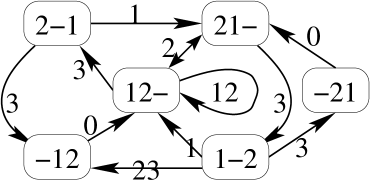
Figure 2. The $b=2$ flag juggling digraph with and only throws $\leq 3$ drawn.

4.1. Another Markov chain

As in §1.2, we define a Markov chain following the edges backwards in this digraph. Let $\widetilde{\tau}$ be a flag juggling state, and again we use a coin with $p($heads$)=1/q$.

1. Hold a $-$, and point at the rightmost number in $\widetilde{\tau}$.

2. Flip the coin. If tails, put down what we’re holding and pick up the number we’re pointing at. If heads, do nothing.

3. Move leftwards; stop when we meet a number smaller than what we’re holding (interpreting $-$ as $+\infty$, jibing with our definition of $\ell(\widetilde{\tau})$).

4. If we meet such a number, go back to (2). Otherwise we’ve fallen off the left end of (the now modified) $\widetilde{\tau}$; drop whatever we’re holding, there.

For example, start with $\widetilde{\tau}=--\ 3\ 1-2$, holding a $-$, pointing at the $2$.

• Tails: pick up the $2$, leaving the $-$ in its place. Point at the $1$.

  • Tails: drop the $2$ for the $1$, then carried all the way left to give $1--\ 3\ 2--$.

  • Heads: the $2$ gets carried all the way left to give $2--\ 3\ 1--$.

• Heads: skip the $2$ and point at the $1$.

  • Tails: pick up the $1$, leaving the $-$, and carry the $1$ all the way left to give $1--\ 3--\ 2$.

  • Heads: leave the $1$ and proceed to the $3$.

    • Tails: pick up the $3$ and carry it left to give $3---1-2$.

    • Heads: leave the $3$ and drop the $-$ on the left, giving $---\ 3\ 1-2$.

$$\text{In all, }\widetilde{\tau} \mapsto (1-q^{-1})^{2}[1--3\ 2]\ +\ (1-q^{-1})q^{-1}\left([2--3\ 1--]+[1--3--2]\right)$$

$$+q^{-2}(1-q^{-1})[3---1-2]\ +\ q^{-3}[---3\ 1-2]$$

This is again motivated by the “add a random column on the left” Markov chain on $U_{b}$:

Proposition 5.

Let $M$ be the partial permutation matrix in $U_{b}$ with $\widetilde{\sigma}(M)=\widetilde{\tau}$, and $\vec{c}$ a random column vector. Then the probability of $\widetilde{\sigma}([\vec{c}M])$ being a particular state $\tau^{\prime}$ is the probability of reaching $\tau^{\prime}$ in the process above.

In particular, the possible $\tau^{\prime}$ are the ones such that $\tau^{\prime}\to\tau$ in the digraph defined in this section.

Proof sketch.

Rightward column-reduction of $[\vec{c}\ M]$ corresponds to doing the coin flips, in reverse order. At each coin-flipping step, we determine that a certain entry of $\vec{c}$ is zero (heads) or nonzero (tails). We leave the details to the reader. ∎

We have the corresponding theorem, but skip the corresponding formal derivation:

Theorem 2.

The vector $\widetilde{\tau}\mapsto(1-q^{-1})^{b}q^{-\ell(\widetilde{\tau})}$ is the stationary distribution of the Markov chain (1)-(4) defined above.

4.2. The linear algebra of repeated labels

Given a finite multiset $S$ of numbers, we can redefine flag juggling states to bear those labels, and the Markov chain in this section extends without changing a word. If the elements of $S$ are all equal, or all different, we get the digraphs from §1 and §4 respectively. So one can ask for a corresponding linear algebra problem and, hopefully thereby, calculation of the stationary distribution.

To interpolate between all row operations and downward row operations, we consider the rows as coming in contiguous groups, and only allow row operations within a group or downward. For example if $S=\{1,1,5,7,7,7\}$, then we have three groups, which are two rows above one row above three rows.

In the analogue of reduced row-echelon form, the $b$ pivot columns are still arbitrary, but the pivots within a given group run Northwest/Southeast. In the analogue of corollaries 1 and 2, the prefactor is

$$\prod^{\text{groups}}\prod_{i=1}^{\text{group size}}(1-q^{-i})$$

which computes the probability that a block lower triangular matrix is invertible. These prefactors, times $q^{-\ell(\widetilde{\tau})}$, again give the stationary distribution.

5. Drawing out the process

Since the transitions in the (flag) juggling Markov chain involve repeated flipping of coins, it seems natural to ask for an alternative version with intermediate states, such that only one coin is flipped at each transition.

5.1. The digraph of ordinary and hatted states

Define a hatted flag juggling state $\tau_{+}$ as a flag juggling state $\tau$ with one position hatted, as in $\hat{5}$ or $\hat{-}$. The hat is not allowed over one of the $-$s occurring after $\tau$’s last number, e.g. $3-4--\ldots$ can only be hatted as $\hat{3}-4$, $3\hat{-}4$, or $3-\hat{4}$.

The vertices of the digraph will be the usual unaugmented states, plus these new, intermediate, states. Make directed edges as follows:

• If $\tau$ is unhatted, then it has only one arrow out, hatting the $0$th label.
  Example: $\qquad 3-\ 2\ 1\quad\to\quad\hat{3}-\ 2\ 1$.

• If $\tau_{+}$ has a hat, then there are one or two arrows out of $\tau_{+}$.

  • We can move the hat and label one step rightward, switching places with the unhatted label just beyond, unless that involves switching a $\hat{-}$ with the last number in $\tau$.  Example:   $\hat{3}-\ 2\ 1\quad\to\quad-\ \hat{3}\ 2\ 1$.

  • If the hatted label is the last number in $\tau$, we can remove the hat. If it isn’t, and the next label after the hatted label is larger (counting $-$ as $\infty$), then the hat can jump one step rightward to that larger label, with the labels not moving.
    Example:   $\hat{3}-\ 2\ 1\quad\to\quad 3\ \hat{-}\ 2\ 1\quad\cancel{\to}\quad 3-\hat{2}\ 1$.

It’s easy to see that if $\tau,\tau^{\prime}$ are unhatted states, then $\tau\to\tau^{\prime}$ in the digraph from §4 iff there is a directed path in this digraph from $\tau$ to $\tau^{\prime}$ through only hatted states.

5.2. The last Markov chain

As twice before, we put probabilities on the reversed edges.

If $\tau$ is an unhatted state, the only edge into it has a hat on the last number in $\tau$. Whereas if $\tau_{+}$ is $\tau$ with a hat at position $0$, the only edge into $\tau_{+}$ comes from $\tau$. In either case the unique edge gets probability $1$.

In the remaining case, $\tau_{+}$ has a hat at position $i>0$, and we must move the hat left one step. If the label to the left is smaller than the hatted label, then we move the hat left with probability $1$ and are done. But if that label is larger, then with probability $1/q$, we move the label bearing the hat, not just the hat. From the state $3\ -2\ \hat{1}$:

$$3\ -\hat{2}\ 1\qquad\stackrel{{\scriptstyle 1-q^{-1}}}{{\longrightarrow}}\qquad 3\ -2\ \hat{1}\qquad\stackrel{{\scriptstyle q^{-1}}}{{\longleftarrow}}\qquad 3\ -\hat{1}\ 2$$

(Don’t forget that the Markov chain runs backwards along the arrows.)

Again, we claim that if $\tau,\tau^{\prime}$ are unhatted states, and we start this Markov chain at $\tau$ and stop when we next meet an unhatted state, the probability that it is $\tau^{\prime}$ is the same as that given by the Markov chain from §4.

6. Questions

What is a linear algebra interpretation of the model in §5?

Is there an analogue of [BEGW94] for the flag juggling digraph?

The stationary distributions computed here live on $S_{b+{\mathbb{N}}}/(S_{b}\times S_{\mathbb{N}})$ and $S_{b+{\mathbb{N}}}/((S_{1})^{b}\times S_{\mathbb{N}})$, and easily generalize to other $W/W_{P}$ coset spaces ($\tau\mapsto q^{-\ell(\tau)}$ times a prefactor). What is a Markov chain on $W/W_{P}$ for which they are the stationary distribution?

What is an analogue of the ball density function calculated in §3, when the balls are colored as in §4?

Is there a version of §1 in which $b$ varies, whose stationary distribution is still $q^{-\text{area}}$, up to overall scale? Does that have a linear algebra interpretation?

Is the $q\to 1$ limit related in any substantive way to the mythical field of $1$ element? Can that theoretical theory include the $b\to\infty$ limit?

It is easy to define a version of the digraph from §5 with multiple hatted labels percolating through independently. Is this of any use?

References

- [ABCN] Arvind Ayyer, Jérémie Bouttier, Sylvie Corteel, François Nunzi, Multivariate juggling probabilities. Preprint 2014. http://arxiv.org/abs/1402.3752
- [ABCLN] Arvind Ayyer, Jérémie Bouttier, Sylvie Corteel, Svante Linusson, François Nunzi, Bumping sequences and multispecies juggling. Preprint 2015. http://arxiv.org/abs/1504.02688
-
[BEGW94]
Joe Buhler, David Eisenbud, Ron Graham, and Colin Wright,
Juggling drops and descents. American Mathematical Monthly 101 (1994) 507–519.
Reprinted with new appendix in the Canadian Mathematical Society, Conference Proceedings,
Volume 20, 1997. http://www.math.ucsd.edu/~ronspubs/94_01a_juggling.pdf -
[BG10]
Steve Butler, Ron Graham,
Enumerating (multiplex) juggling sequences.
Annals of Combinatorics 13 (2010), 413–424.
http://www.math.ucsd.edu/~ronspubs/10_03_multiplex.pdf -
[CG08]
F.R.K. Chung, Ron Graham,
Primitive juggling sequences.
American Mathematical Monthly 115 (March 2008), 185–194.
http://www.math.ucsd.edu/~ronspubs/08_03_primitive_juggling.pdf -
[ER96]
Richard Ehrenborg, Margaret Readdy,
Juggling and applications to -analogues.
Discrete Math. 157 (1996), 107–125. http://www.ms.uky.edu/~jrge/Papers/Juggle.pdf -
[ELV15]
Alexander Engström, Lasse Leskelä, Harri Varpanen.
Geometric juggling with -analogues.
Discrete Mathematics 338 (2015), pp. 1067–1074. http://arxiv.org/abs/1310.2725 -
[KLS13]
Allen Knutson, David E Speyer, and Thomas Lam,
Positroid varieties: juggling and geometry. Compositio Mathematica 149, Issue 10, (October 2013), pp. 1710–1752. http://arxiv.org/abs/1111.3660 -
[LV12]
Lasse Leskelä, Harri Varpanen,
Juggler’s exclusion process.
Journal of Applied Probability 49(1), 2012, pp. 266–-279. http://arxiv.org/abs/1104.3397 - [Pol03] Burkhard Polster, The mathematics of juggling. Springer-Verlag, New York, 2003.
-
[Pos]
Alexander Postnikov,
Total positivity, Grassmannians, and networks.
http://arxiv.org/abs/math/0609764 - [Va14] Harri Varpanen, Toss and spin juggling state graphs. Proceedings of Bridges 2014, pp. 301–308, 2014. http://arxiv.org/abs/1405.2628
- [Wa05] Greg Warrington, Juggling probabilities. American Mathematical Monthly 112, no. 2 (2005), 105–118. http://arxiv.org/abs/math/0302257