Crystallizing the hypoplactic monoid: from quasi-Kashiwara operators to the Robinson–Schensted–Knuth-type correspondence for quasi-ribbon tableaux

Abstract.

Crystal graphs, in the sense of Kashiwara, carry a natural monoid structure given by identifying words labelling vertices that appear in the same position of isomorphic components of the crystal. In the particular case of the crystal graph for the $q$-analogue of the special linear Lie algebra $\mathfrak{sl}_{n}$, this monoid is the celebrated plactic monoid, whose elements can be identified with Young tableaux. The crystal graph and the so-called Kashiwara operators interact beautifully with the combinatorics of Young tableaux and with the Robinson–Schensted–Knuth correspondence and so provide powerful combinatorial tools to work with them. This paper constructs an analogous ‘quasi-crystal’ structure for the hypoplactic monoid, whose elements can be identified with quasi-ribbon tableaux and whose connection with the theory of quasi-symmetric functions echoes the connection of the plactic monoid with the theory of symmetric functions. This quasi-crystal structure and the associated quasi-Kashiwara operators are shown to interact just as neatly with the combinatorics of quasi-ribbon tableaux and with the hypoplactic version of the Robinson–Schensted–Knuth correspondence. A study is then made of the interaction of the crystal graph of the plactic monoid and the quasi-crystal graph for the hypoplactic monoid. Finally, the quasi-crystal structure is applied to prove some new results about the hypoplactic monoid.

1. Introduction

A crystal basis, in the sense of Kashiwara [Kas91, Kas90], is (informally) a basis for a representation of a suitable algebra on which the generators have a particularly neat action. It gives rise, via tensor products, to the crystal graph, which carries a natural monoid structure given by identifying words labelling vertices that appear in the same position of isomorphic components. The ubiquitous plactic monoid, whose elements can be viewed as semistandard Young tableaux, and which appears in such diverse contexts as symmetric functions [Mac95], representation theory and algebraic combinatorics [Ful97, Lot02], Kostka–Foulkes polynomials [LS81, LS78], Schubert polynomials [LS85, LS90], and musical theory [Jed11], arises in this way from the crystal basis for the $q$-analogue of the special linear Lie algebra $\mathfrak{sl}_{n}$. The crystal graph and the associated Kashiwara operators interact beautifully with the combinatorics of Young tableaux and with the Robinson–Schensted–Knuth correspondence and so provide powerful combinatorial tools to work with them.

This paper is dedicated to constructing an analogue of this crystal structure for the monoid of quasi-ribbon tableaux: the so-called hypoplactic monoid. To explain this aim in more detail, and in particular to describe the properties such an analogue should enjoy, it is necessary to briefly recapitulate some of the theory of crystals and of Young tableaux.

The plactic monoid of rank $n$ (where $n\in\mathbb{N}$) arises by factoring the free monoid $\mathcal{A}_{n}^{*}$ over the ordered alphabet $\mathcal{A}_{n}=\{1<\ldots<n\}$ by a relation $\equiv_{\smash{\mathrm{plac}}}$, which can be defined in various ways. Using Schensted’s algorithm [Sch61], which was originally intended to find longest increasing and decreasing subsequences of a given sequence, one can compute a (semistandard) Young tableau $\mathrm{P}\lparen w\rparen$ from a word $w\in\mathcal{A}_{n}^{*}$ and so define $\equiv_{\smash{\mathrm{plac}}}$ as relating those words that yield the same Young tableau. Knuth made a study of correspondences between Young tableaux and non-negative integer matrices and gave defining relations for the plactic monoid [Knu70]; the relation $\equiv_{\smash{\mathrm{plac}}}$ can be viewed as the congruence generated by these defining relations.

Lascoux & Schützenberger [LS81] began the systematic study of the plactic monoid, and, as remarked above, connections have emerged with myriad areas of mathematics, which is one of the reasons Schützenberger proclaimed it ‘one of the most fundamental monoids in algebra’ [Sch97]. Of particular interest for us is how it arises from the crystal basis for the $q$-analogue of the special linear Lie algebra $\mathfrak{sl}_{n}$ (that is, the type $A_{n+1}$ simple Lie algebra), which links it to Kashiwara’s theory of crystal bases [KN94]. Isomorphisms between connected components of the crystal graph correspond to the relation $\equiv_{\smash{\mathrm{plac}}}$. Viewed on a purely combinatorial level, the Kashiwara operators and crystal graph are important tools for working with the plactic monoid. (Indeed, in this context they are sometimes called ‘coplactic’ operators [Lot02, ch. 5], being in a sense ‘orthogonal’ to $\equiv_{\smash{\mathrm{plac}}}$.) Similarly, crystal theory can also be used to analyse the analogous ‘plactic monoids’ that index representations of the $q$-analogues of symplectic Lie algebras $\mathfrak{sp}_{n}$ (the type $C_{n}$ simple Lie algebra), special orthogonal Lie algebras of odd and even rank $\mathfrak{so}_{2n+1}$ and $\mathfrak{so}_{2n}$ (the type $B_{n}$ and $D_{n}$ simple Lie algebras), and the exceptional simple Lie algebra $G_{2}$ (see [KS04, Lec02, Lec03] and the survey [Lec07]). The present authors and Gray applied this crystal theory to construct finite complete rewriting systems and biautomatic structures for all these plactic monoids [CGM]; Hage independently constructed a finite complete rewriting system for the plactic monoid of type $C_{n}$ [Hag15].

As is described in detail later in the paper, the crystal structure meshes neatly with the Robinson–Schensted–Knuth correspondence. This correspondence is a bijection $w\leftrightarrow(P,Q)$ where $w$ is a word over $\mathcal{A}_{n}$, and $P$ is a semistandard Young tableau with entries in $\mathcal{A}_{n}$ and $Q$ is a standard Young tableau of the same shape. (The semistandard Young tableau $P$ is the tableau $\mathrm{P}\lparen w\rparen$ computed by Schensted’s algorithm; the standard tableau $Q$ can be computed in parallel.) Essentially, the standard Young tableau $Q$ corresponds to the connected component of the crystal graph in which the word $w$ lies, and the semistandard Young tableau $P$ corresponds to the position of $w$ in that component. By holding $Q$ fixed and varying $P$ over semistandard tableaux of the same shape, one obtains all words in a given connected component. Consequently, all words in a given connected component correspond to tableaux of the same shape.

In summary, there are three equivalent approaches to the plactic monoid:

• Generators and relations: the plactic monoid is defined by the presentation $\big{\langle}\,\mathcal{A}_{n}\,\big{|}\,\mathopen{}\mathcal{R}_{\smash{\mathrm{plac}}}\,\big{\rangle}$, where

  $$\mathcal{R}_{\smash{\mathrm{plac}}}={} \big{\{}\,(acb,cab):a\leq b<c\,\big{\}}$$

  $$\cup\big{\{}\,(bac,bca):a<b\leq c\,\big{\}}.$$

  Equivalently, $\equiv_{\smash{\mathrm{plac}}}$ is the congruence on $\mathcal{A}_{n}^{*}$ generated by $\mathcal{R}_{\smash{\mathrm{plac}}}$.

• Tableaux and insertion: the relation $\equiv_{\smash{\mathrm{plac}}}$ is defined by $u\equiv_{\smash{\mathrm{plac}}}v$ if and only if $\mathrm{P}\lparen u\rparen=\mathrm{P}\lparen v\rparen$, where $\mathrm{P}\lparen\cdot\rparen$ is the Young tableau computed using the Schensted insertion algorithm (see Algorithm 3.2 below).

• Crystals: the relation $\equiv_{\smash{\mathrm{plac}}}$ is defined by $u\equiv_{\smash{\mathrm{plac}}}v$ if and only if there is a crystal isomorphism between connected components of the crystal graph that maps $u$ onto $v$.

The defining relations in $\mathcal{R}_{\smash{\mathrm{plac}}}$ (known as the Knuth relations) are the reverse of the ones given in [CGM]. This is because, in the context of crystal bases, the convention for tensor products gives rise to a ‘plactic monoid’ that is actually anti-isomorphic to the usual notion of plactic monoid. Since this paper is mainly concerned with combinatorics, rather than representation theory, it follows Shimozono [Shi05] in using the convention that is compatible with the usual notions of Young tableaux and the Robinson–Schensted–Knuth correspondence.

Another important aspect of the plactic monoid is its connection to the theory of symmetric polynomials. The Schur polynomials with $n$ indeterminates, which are the irreducible polynomial characters of the general linear group $\mathrm{GL}_{n}(\mathbb{C})$, are indexed by shapes of Young tableaux with entries in $\mathcal{A}_{n}$, and they form a $\mathbb{Z}$-basis for the ring of symmetric polynomials in $n$ indeterminates. The plactic monoid was applied to give the first rigorous proof of the Littlewood–Richardson rule (see [LR34] and [Gre07, Appendix]), which is a combinatorial rule for expressing a product of two Schur polynomials as a linear combination of Schur polynomials.

In recent years, there has emerged a substantial theory of non-commutative symmetric functions and quasi-symmetric functions; see, for example, [GKL⁺95, KT97, KT99]. Of particular interest for this paper is the notion of quasi-ribbon polynomials, which form a basis for the ring of quasi-symmetric polynomials, just as the Schur polynomials form a basis for the ring of symmetric polynomials. The quasi-ribbon polynomials are indexed by the so-called quasi-ribbon tableaux. These quasi-ribbon tableaux have an insertion algorithm and an associated monoid called the hypoplactic monoid, which was first studied in depth by Novelli [Nov00]. The hypoplactic monoid of rank $n$ arises by factoring the free monoid $\mathcal{A}_{n}^{*}$ by a relation $\equiv_{\smash{\mathrm{hypo}}}$, which, like $\equiv_{\smash{\mathrm{plac}}}$, can be defined in various ways. Using the insertion algorithm one can compute a quasi-ribbon tableau from a word and so define $\equiv_{\smash{\mathrm{hypo}}}$ as relating those words that yield the same quasi-ribbon tableau. Alternatively, the relation $\equiv_{\smash{\mathrm{hypo}}}$ can be viewed as the congruence generated by certain defining relations.

Thus there are two equivalent approaches to the hypoplactic monoid:

• Generators and relations: the hypoplactic monoid is defined by the presentation $\big{\langle}\,\mathcal{A}_{n}\,\big{|}\,\mathopen{}\mathcal{R}_{\smash{\mathrm{hypo}}}\,\big{\rangle}$, where

  $$\mathcal{R}_{\smash{\mathrm{hypo}}}={} \mathcal{R}_{\smash{\mathrm{plac}}}$$

  $$\cup\big{\{}\,(cadb,acbd):a\leq b<c\leq d\,\big{\}}$$

  $$\cup\big{\{}\,(bdac,dbca):a<b\leq c<d\,\big{\}}.$$

  Equivalently, $\equiv_{\smash{\mathrm{hypo}}}$ is the congruence on the free monoid $\mathcal{A}_{n}^{*}$ generated by $\mathcal{R}_{\smash{\mathrm{hypo}}}$.

• Tableaux and insertion: the relation $\equiv_{\smash{\mathrm{hypo}}}$ is defined by $u\equiv_{\smash{\mathrm{hypo}}}v$ if and only if $\mathrm{QR}\lparen u\rparen=\mathrm{QR}\lparen v\rparen$, where $\mathrm{QR}\lparen{\cdot}\rparen$ is the quasi-ribbon tableau computed using the Krob–Thibon insertion algorithm (see Algorithm 4.3 below).

Krob & Thibon [KT97] proved the equivalence of H1 and H2, which are the direct analogues of P1 and P2. Owing to the previous success in detaching crystal basis theory from its representation-theoretic foundation and using it as a combinatorial tool for working with Young tableaux and plactic monoids, it seems worthwhile to try to find an analogue of P3 for the hypoplactic monoid. Such an analogue should have the following form:

• Quasi-crystals: the relation $\equiv_{\smash{\mathrm{hypo}}}$ is defined by $u\equiv_{\smash{\mathrm{hypo}}}v$ if and only if there is a quasi-crystal isomorphism between connected components of the quasi-crystal graph that maps $u$ onto $v$.

The aim of this paper is to define quasi-Kashiwara operators on a purely combinatorial level, and so construct a quasi-crystal graph as required for H3. As will be shown, the interaction of the combinatorics of quasi-ribbon tableaux with this quasi-crystal graph will be a close analogue of the interaction of the combinatorics of Young tableaux with the crystal graph (and is, in the authors’ view, just as elegant).

In fact, a related notion of ‘quasi-crystal’ is found in Krob & Thibon [KT99]; see also [Hiv00]. However, the Krob–Thibon quasi-crystal describes the restriction to quasi-ribbon tableaux (or more precisely words corresponding to quasi-ribbon tableaux) of the action of the usual Kashiwara operators: it does not apply to all words and so does not give rise to isomorphisms that can be used to define the relation $\equiv_{\smash{\mathrm{hypo}}}$.

The paper is organized as follows: Section 2 sets up notation and discusses some preliminaries relating to words, partitions, compositions, and the notion of weight. Section 3 reviews, without proof, the basic theory of Young tableaux, the plactic monoid, Kashiwara operators, and the crystal graph; the aim is to gather the elegant properties of the crystal structure for the plactic monoid that should be mirrored in the quasi-crystal structure for the hypoplactic monoid. These properties will also be used in the study of the interactions of the crystal and quasi-crystal graphs. Section 4 recalls the definitions of quasi-ribbon tableaux and the hypoplactic monoid. Section 5 states the definition of the quasi-Kashiwara operators and the quasi-crystal graph, and shows that isomorphisms between connected components of this quasi-crystal graph give rise to a congruence on the free monoid. Section 6 proves that the corresponding factor monoid is the hypoplactic monoid. En route, some of the properties of the quasi-crystal graph are established. Section 7 studies how the quasi-crystal graph interacts with the hypoplactic version of the Robinson–Schensted–Knuth correspondence. Section 8 systematically studies the structure of the quasi-crystal graph. It turns out to be a subgraph of the crystal graph for the plactic monoid, and the interplay of the subgraph and graph has some very neat properties. Finally, the quasi-crystal structure is applied to prove some new results about the hypoplactic monoid in Section 9, including an analogy of the hook-length formula.

2. Preliminaries and notation

2.1. Alphabets and words

Recall that for any alphabet $X$, the free monoid (that is, the set of all words, including the empty word) on the alphabet $X$ is denoted $X^{*}$. The empty word is denoted $\varepsilon$. For any $u\in X^{*}$, the length of $u$ is denoted $|u|$, and, for any $x\in X$, the number of times the symbol $x$ appears in $u$ is denoted $|u|_{x}$. Suppose $u=u_{1}\cdots u_{k}\in X^{*}$ (where $u_{h}\in X$). For any $i\leq j$, the word $u_{i}\cdots u_{j}$ is a factor of $u$. For any $i_{1},\ldots,i_{m}\in\{1,\ldots,k\}$ such that $i_{1}<i_{2}<\ldots<i_{m}$, the word $u_{i_{1}}u_{i_{2}}\cdots u_{i_{m}}$ is a subsequence of $u$. Note that factors must be made up of consecutive letters, whereas subsequences may be made up of non-consecutive letters. [To minimize potential confusion, the term ‘subword’ is not used in this paper, since it tends to be synonymous with ‘factor’ in semigroup theory, but with ‘subsequence’ in combinatorics on words.]

For further background on the free monoid, see [How95]; for presentations, see [Hig92, Ruš95].

Throughout this paper, $\mathcal{A}$ will be the set of natural numbers viewed as an infinite ordered alphabet: $\mathcal{A}=\{1<2<3<\ldots\}$. Further, $n$ will be a natural number and $\mathcal{A}_{n}$ will be the set of the first $n$ natural numbers viewed as an ordered alphabet: $\mathcal{A}_{n}=\{1<2<\ldots<n\}$.

A word $u\in\mathcal{A}^{*}$ is standard if it contains each symbol in $\{1,\ldots,|u|\}$ exactly once. Let $u=u_{1}\cdots u_{k}$ be a standard word. The word $u$ is identified with the permutation $h\mapsto u_{h}$, and $u^{-1}$ denotes the inverse of this permutation (which is also identifed with a standard word).

Further, the descent set of the standard word $u$ is $D(u)=\big{\{}\,h\in\{1,\ldots,|u|-1\}:u_{h}>u_{h+1}\,\big{\}}$.

Let $u\in\mathcal{A}^{*}$. The standardization of $u$, denoted $\mathrm{std}\lparen u\rparen$, is the standard word obtained by the following process: read $u$ from left to right and, for each $a\in\mathcal{A}$, attach a subscript $h$ to the $h$-th appearance of $a$. Symbols with attached subscripts are ordered by

$$a_{i}<b_{j}\iff\lparen a<b\rparen\lor\big{\lparen}\lparen a=b\rparen\land\lparen i<j\rparen\big{\rparen}.$$

Replace each symbol with an attached subscript in $u$ with the corresponding symbol of the same rank from $\mathcal{A}$. The resulting word is $\mathrm{std}\lparen u\rparen$. For example:

$$w={} \mathrlap{2}\phantom{2_{1}}\mathrlap{4}\phantom{4_{1}}\mathrlap{3}\phantom{3_{1}}\mathrlap{2}\phantom{2_{2}}\mathrlap{4}\phantom{4_{1}}\mathrlap{5}\phantom{5_{1}}\mathrlap{5}\phantom{5_{2}}\mathrlap{6}\phantom{6_{1}}\mathrlap{5}\phantom{5_{3}}$$

$$\rightsquigarrow{} 2_{1}4_{1}3_{1}2_{2}4_{2}5_{1}5_{2}6_{1}5_{3}$$

$$\mathrm{std}\lparen w\rparen={} \mathrlap{1}\phantom{2_{1}}\mathrlap{4}\phantom{4_{1}}\mathrlap{3}\phantom{3_{1}}\mathrlap{2}\phantom{2_{2}}\mathrlap{5}\phantom{4_{1}}\mathrlap{6}\phantom{5_{1}}\mathrlap{7}\phantom{5_{2}}\mathrlap{9}\phantom{6_{1}}\mathrlap{8}\phantom{5_{3}}$$

For further background relating to standard words and standardizaton, see [Nov00, § 2].

2.2. Compositions and partitions

A weak composition $\alpha$ is a finite sequence $(\alpha_{1},\ldots,\alpha_{m})$ with terms in $\mathbb{N}\cup\{0\}$. The terms $\alpha_{h}$ up to the last non-zero term are the parts of $\alpha$. The length of $\alpha$, denoted $\ell\lparen\alpha\rparen$, is the number of its parts. The weight of $\alpha$, denoted $\lvert\alpha\rvert$, is the sum of its parts (or, equivalently, of its terms): $\lvert\alpha\rvert=\alpha_{1}+\cdots+\alpha_{m}$. For example, if $\alpha=(3,0,4,1,0)$, then $\ell\lparen\alpha\rparen=4$ and $\lvert\alpha\rvert=8$. Identify weak compositions whose parts are the same (that is, that differ only in a tail of terms $0$). For example, $(3,1,5,2)$ is identified with $(3,1,5,2,0)$ and $(3,1,5,2,0,0,0)$. (Note that this identification does not create ambiguity in the notions of parts and weight.) A composition is a weak composition whose parts are all in $\mathbb{N}$. For a composition $\alpha=(\alpha_{1},\ldots,\alpha_{\ell\lparen\alpha\rparen})$, define $D(\alpha)=\{\alpha_{1},\alpha_{1}+\alpha_{2},\ldots,\alpha_{1}+\ldots+\alpha_{\ell\lparen\alpha-\rparen 1}\}$. For a standard word $u\in\mathcal{A}^{*}$, define $\mathcal{DC}\lparen u\rparen$ to be the unique composition of weight $\lvert u\rvert$ such that $D(\mathcal{DC}\lparen u\rparen)=D(u)$, where $D(u)$ is as defined in Subsection 2.1. For example, if $u=143256798$, then $D(u)=\{2,3,8\}$ and so $\mathcal{DC}\lparen u\rparen=(2,1,5,1)$.

A partition $\lambda$ is a non-increasing finite sequence $(\lambda_{1},\ldots,\lambda_{m})$ with terms in $\mathbb{N}$. The terms $\lambda_{h}$ are the parts of $\lambda$. The length of $\lambda$, denoted $\ell\lparen\lambda\rparen$, is the number of its parts. The weight of $\lambda$, denoted $\lvert\lambda\rvert$, is the sum of its parts: $\lvert\lambda\rvert=\lambda_{1}+\cdots+\lambda_{m}$. For example, if $\lambda=(5,3,2,2)$, then $\ell\lparen\lambda\rparen=4$ and $\lvert\lambda\rvert=12$.

2.3. Weight

The weight function $\mathrm{wt}$ is, informally, the function that counts the number of times each symbol appears in a word. More formally, $\mathrm{wt}$ is defined by

$$\mathrm{wt}:\mathcal{A}^{*}\to(\mathbb{N}\cup\{0\})^{\mathcal{A}}\qquad u\mapsto\big{\lparen}|u|_{1},|u|_{2},|u|_{3},\ldots\big{\rparen}.$$

Clearly, $\mathrm{wt}\lparen\cdot\rparen$ has an infinite tail of components $0$, so only the prefix up to the last non-zero term is considered; thus $\mathrm{wt}\lparen\cdot\rparen$ is a weak composition. For example, $\mathrm{wt}\lparen 542164325224\rparen=(1,4,1,3,2,1)$. See [Shi05, § 2.1] for a discussion of the basic properties of weight functions.

Weights are compared using the following order:

(2.1) $$(\alpha_{1},\alpha_{2},\ldots)\leq(\beta_{1},\beta_{2},\ldots)$$

$$\qquad\iff(\forall k\in\mathbb{N})\Big{\lparen}\sum_{i=1}^{k}\alpha_{i}\leq\sum_{i=1}^{k}\beta_{i}\Big{\rparen}.$$

When $\lvert\alpha\rvert=\lvert\beta\rvert$, this is the dominance order of partitions [Sta05, § 7.2]. When $\mathrm{wt}\lparen u\rparen<\mathrm{wt}\lparen v\rparen$, one says that $v$ has higher weight than $u$ (and $u$ has lower weight than $v$). For example,

$$\mathrm{wt}\lparen 542164325224\rparen=(1,4,1,3,2,1)\\ <(5,3,2,2,0,0)=\mathrm{wt}\lparen 432143212111\rparen;$$

that is, $432143212111$ has higher weight than $542164325224$. For the purposes of this paper, it will generally not be necessary to compare weights using (2.1); the important fact will be how the Kashiwara operators affect weight.

3. Crystals and the plactic monoid

This section recalls in detail the three approaches to the plactic monoid discussed in the introduction, and discusses further the very elegant interaction of the crystal structure with the combinatorics of Young tableaux and in particular with the Robinson–Schensted–Knuth correspondence. The aim is to lay out the various properties one would hope for in the quasi-crystal structure for the hypoplactic monoid.

3.1. Young tableaux and insertion

The Young diagram of shape $\lambda$, where $\lambda$ is a partition, is a grid of boxes, with $\lambda_{h}$ boxes in the $h$-th row, for $h=1,\ldots,\ell\lparen\lambda\rparen$, with rows left-aligned. For example, the Young diagram of shape $(5,3,2,2)$ is

A Young diagram of shape $(1,1,\ldots,1)$ is said to be a column diagram or to have column shape. Note that, in this paper, Young diagrams are top-left aligned, with longer rows at the top and the parts of the partition specifying row lengths from top to bottom. There is an alternative convention of bottom-left aligned Young diagrams, where longer rows are at the bottom.

A Young tableau is a Young diagram that is filled with symbols from $\mathcal{A}$ so that the entries in each row are non-decreasing from left to right, and the entries in each column are increasing from top to bottom. For example, a Young tableau of shape $(5,3,2,2)$ is

(3.1)

A Young tableau of shape $(1,1,\ldots,1)$ is a column. (That is, a column is a Young tableau of column shape.)

A standard Young tableau of shape $\lambda$ is a Young diagram that is filled with symbols from $\{1,\ldots,\lvert\lambda\rvert\}$, with each symbol appearing exactly once, so that the entries in each row are increasing from left to right, and the entries in each column are increasing from top to bottom. For example, a standard Young tableau of shape $(5,3,2,2)$ is

A tabloid is an array formed by concatenating columns, filled with symbols from $\mathcal{A}$ so that the entries in each column are increasing from top to bottom. (Notice that there is no restriction on the relative heights of the columns; nor is there a condition on the order of entries in a row.) An example of a tabloid is

(3.2)

Note that a tableau is a special kind of tabloid. The shape of a tabloid cannot in general be expressed using a partition.

The column reading $\mathrm{C}\lparen T\rparen$ of a tabloid $T$ is the word in $\mathcal{A}^{*}$ obtained by proceeding through the columns, from leftmost to rightmost, and reading each column from bottom to top. For example, the column readings of the tableau (3.1) and the tabloid (3.2) are respectively $5421\,6432\,52\,2\,4$ and $52\,6431\,4\,5421\,2$ (where the spaces are simply for clarity, to show readings of individual columns), as illustrated below:

      

Let $w\in\mathcal{A}^{*}$, and let $w^{(1)}\cdots w^{(m)}$ be the factorization of $w$ into maximal decreasing factors. Let $\mathrm{Toid}\lparen w\rparen$ be the tabloid whose $h$-th column has height $|w^{(h)}|$ and is filled with the symbols of $w^{(h)}$, for $h=1,\ldots,m$. Then $\mathrm{C}\lparen\mathrm{Toid}\lparen w\rparen\rparen=w$. (Note that the notion of reading described here is the one normally used in the study of Young tableaux and the plactic monoid, and is the opposite of the ‘Japanese reading’ used in the theory of crystals. Throughout the paper, definitions follow the convention compatible with the reading defined here. The resulting differences from the usual practices in crystal theory will be explicitly noted.)

If $w$ is the column reading of some Young tableau $T$, it is called a tableau word. Note that not all words in $\mathcal{A}^{*}$ are tableau words. For example, $343$ is not a tableau word, since and are the only tableaux containing the correct symbols, and neither of these has column reading $343$. The word $w$ is a tableau word if and only if $\mathrm{Toid}\lparen w\rparen$ is a tableau.

The plactic monoid arises from an algorithm that computes a Young tableau $\mathrm{P}\lparen w\rparen$ from a word $w\in\mathcal{A}^{*}$.

Algorithm 3.1 (Schensted’s algorithm).

Input: A Young tableau $T$ and a symbol $a\in\mathcal{A}$.

Output: A Young tableau $T\leftarrow a$.

Method:

1. If $a$ is greater than or equal to every entry in the topmost row of $T$, add $a$ as an entry at the rightmost end of $T$ and output the resulting tableau.

2. Otherwise, let $z$ be the leftmost entry in the top row of $T$ that is strictly greater than $a$. Replace $z$ by $a$ in the topmost row and recursively insert $z$ into the tableau formed by the rows of $T$ below the topmost. (Note that the recursion may end with an insertion into an ‘empty row’ below the existing rows of $T$.)

Using an iterative form of this algorithm, one can start from a word $a_{1}\cdots a_{k}$ (where $a_{i}\in\mathcal{A}$) and compute a Young tableau $\mathrm{P}\lparen a_{1}\cdots a_{k}\rparen$. Essentially, one simply starts with the empty tableau and inserts the symbols $a_{1}$, …, $a_{k}$ in order: However, the algorithm described below also computes a standard Young tableau $\mathrm{Q}\lparen a_{1}\cdots a_{k}\rparen$ that is used in the Robinson–Schensted–Knuth correspondence, which will shortly be described:

Algorithm 3.2.

Input: A word $a_{1}\cdots a_{k}$, where $a_{i}\in\mathcal{A}$.

Output: A Young tableau $\mathrm{P}\lparen a_{1}\cdots a_{k}\rparen$ and a standard Young tableau $\mathrm{Q}\lparen a_{1}\cdots a_{k}\rparen$.

Method: Start with an empty Young tableau $P_{0}$ and an empty standard Young tableau $Q_{0}$. For each $i=1$, …, $k$, insert the symbol $a_{i}$ into $P_{i-1}$ as per Algorithm 3.1; let $P_{i}$ be the resulting Young tableau. Add a cell filled with $i$ to the standard tableaux $Q_{i-1}$ in the same place as the unique cell that lies in $P_{i}$ but not in $P_{i-1}$; let $Q_{i}$ be the resulting standard Young tableau.

Output $P_{k}$ for $\mathrm{P}\lparen a_{1}\cdots a_{k}\rparen$ and $Q_{k}$ as $\mathrm{Q}\lparen a_{1}\cdots a_{k}\rparen$.

For example, the sequence of pairs $(P_{i},Q_{i})$ produced during the application of Algorithm 4.3 to the word $2213$ is

$$\lparen\;,\;\rparen,\;\big{\lparen}\leavevmode\hbox to14.63pt{\vbox to14.63pt{\text{[drawing]}}},\leavevmode\hbox to14.63pt{\vbox to14.63pt{\text{[drawing]}}}\big{\rparen},\;\left\lparen\leavevmode\hbox to28.85pt{\vbox to14.63pt{\text{[drawing]}}},\leavevmode\hbox to28.85pt{\vbox to14.63pt{\text{[drawing]}}}\right\rparen,\;\\ \left\lparen\leavevmode\hbox to28.85pt{\vbox to29.25pt{\text{[drawing]}}},\leavevmode\hbox to28.85pt{\vbox to29.25pt{\text{[drawing]}}}\right\rparen,\;\left\lparen\leavevmode\hbox to43.08pt{\vbox to29.25pt{\text{[drawing]}}},\leavevmode\hbox to43.08pt{\vbox to29.25pt{\text{[drawing]}}}\right\rparen. {2} {1} {2} {2} {1} {2} {1} {2} {2} {1} {2} {3} {1} {2} {3} {2} {1} {2} {4} {3}$$

Therefore $\mathrm{P}\lparen 4323\rparen=\leavevmode\hbox to43.08pt{\vbox to29.25pt{\text{[drawing]}}}$ and $\mathrm{Q}\lparen 4323\rparen=\leavevmode\hbox to43.08pt{\vbox to29.25pt{\text{[drawing]}}}$. It is straightforward to see that the map $w\mapsto\big{\lparen}P(w),Q(w)\big{\rparen}$ is a bijection between words in $\mathcal{A}^{*}$ and pairs consisting of a Young tableau over $\mathcal{A}$ and a standard Young tableau of the same shape. This is the celebrated Robinson–Schensted–Knuth correspondence (see, for example, [Ful97, Ch. 4] or [Sta05, § 7.11].

The possible definition (approach P2 in the introduction) of the relation $\equiv_{\smash{\mathrm{plac}}}$ using tableaux and insertion is the following:

$$u\equiv_{\smash{\mathrm{plac}}}v\iff\mathrm{P}\lparen u\rparen=\mathrm{P}\lparen v\rparen.$$

Using this as a definition, it follows that $\equiv_{\smash{\mathrm{plac}}}$ is a congruence on $\mathcal{A}^{*}$ [Knu70]. The factor monoid $\mathcal{A}^{*}/{\equiv_{\smash{\mathrm{plac}}}}$ is the plactic monoid and is denoted ${\smash{\mathrm{plac}}}$. The relation $\equiv_{\smash{\mathrm{plac}}}$ is the plactic congruence on $\mathcal{A}^{*}$. The congruence $\equiv_{\smash{\mathrm{plac}}}$ naturally restricts to a congruence on $\mathcal{A}_{n}^{*}$, and the factor monoid $\mathcal{A}_{n}^{*}/{\equiv_{\smash{\mathrm{plac}}}}$ is the plactic monoid of rank $n$ and is denoted ${\smash{\mathrm{plac}}}_{n}$.

If $w$ is a tableau word, then $w=\mathrm{C}\lparen\mathrm{P}\lparen w\rparen\rparen$ and $\mathrm{Toid}\lparen w\rparen=\mathrm{P}\lparen w\rparen$. Thus the tableau words in $\mathcal{A}^{*}$ form a cross-section (or set of normal forms) for ${\smash{\mathrm{plac}}}$, and the tableau words in $\mathcal{A}_{n}^{*}$ form a cross-section for ${\smash{\mathrm{plac}}}_{n}$.

3.2. Kashiwara operators and the crystal graph

The following discussion of crystals and Kashiwara operators is restricted to the context of ${\smash{\mathrm{plac}}}_{n}$. For a more general introduction to crystal bases, see [CGM].

The Kashiwara operators $\tilde{e}_{i}$ and $\tilde{f}_{i}$, where $i\in\{1,\ldots,n-1\}$, are partially-defined operators on $\mathcal{A}_{n}^{*}$. In representation-theoretic terms, the operators $\tilde{e}_{i}$ and $\tilde{f}_{i}$ act on a tensor product by acting on a single tensor factor [HK02, § 4.4]. This action can be described in a combinatorial way using the the so-called signature or bracketing rule. This paper describes the action directly using this rule, since the the analogous quasi-Kashiwara operators are defined by modifying this rule.

The definitions of $\tilde{e}_{i}$ and $\tilde{f}_{i}$ start from the crystal basis for ${\smash{\mathrm{plac}}}_{n}$, which will form a connected component of the crystal graph:

(3.3)

Each operator $\tilde{f}_{i}$ is defined so that it ‘moves’ a symbol $a$ forwards along a directed edge labelled by $i$ whenever such an edge starts at $a$, and each operator $\tilde{e}_{i}$ is defined so that it ‘moves’ a symbol $a$ backwards along a directed edge labelled by $i$ whenever such an edge ends at $a$:

and

Using the crystal basis given above, one sees that

$$\tilde{e}_{i}(i+1) =i, \tilde{e}_{i}(x) x\neq i+1$$ is undefined for ;

$$\tilde{f}_{i}(i) =i+1, \tilde{f}_{i}(x) x\neq i$$ is undefined for .

The definition is extended to $\mathcal{A}_{n}^{*}\setminus\mathcal{A}_{n}$ by the recursion

$$\tilde{e}_{i}(uv) =\begin{cases}\tilde{e}_{i}(u)\,v&\text{if $\tilde{\epsilon}_{i}(u)>\tilde{\phi}_{i}(v)$;}\\ u\,\tilde{e}_{i}(v)&\text{if $\tilde{\epsilon}_{i}(u)\leq\tilde{\phi}_{i}(v)$,}\end{cases}$$

$$\tilde{f}_{i}(uv) =\begin{cases}\tilde{f}_{i}(u)\,v&\text{if $\tilde{\epsilon}_{i}(u)\geq\tilde{\phi}_{i}(v)$;}\\ u\,\tilde{f}_{i}(v)&\text{if $\tilde{\epsilon}_{i}(u)<\tilde{\phi}_{i}(v)$,}\end{cases}$$

where $\tilde{\epsilon}_{i}$ and $\tilde{\phi}_{i}$ are auxiliary maps defined by

$$\tilde{\epsilon}_{i}(w) =\max\big{\{}\,k\in\mathbb{N}\cup\{0\}:\text{$\underbrace{\tilde{e}_{i}\cdots\tilde{e}_{i}}_{\text{$k$ times}}(w)$ is defined}\,\big{\}};$$

$$\tilde{\phi}_{i}(w) =\max\big{\{}\,k\in\mathbb{N}\cup\{0\}:\text{$\underbrace{\tilde{f}_{i}\cdots\tilde{f}_{i}}_{\text{$k$ times}}(w)$ is defined}\,\big{\}}.$$

Notice that this definition is not circular: the definitions of $\tilde{e}_{i}$ and $\tilde{f}_{i}$ depend, via $\tilde{\epsilon}_{i}$ and $\tilde{\phi}_{i}$, only on $\tilde{e}_{i}$ and $\tilde{f}_{i}$ applied to strictly shorter words; the recursion terminates with $\tilde{e}_{i}$ and $\tilde{f}_{i}$ applied to single letters from the alphabet $\mathcal{A}_{n}$, which was defined using the crystal basis (3.3). (Note that this definition is in a sense the mirror image of [KN94, Theorem 1.14], because of the choice of definition for readings of tableaux used in this paper. Thus the definition of $\tilde{e}_{i}$ and $\tilde{f}_{i}$ is the same as [Shi05, p. 8].)

Although it is not immediate from the definition, the operators $\tilde{e}_{i}$ and $\tilde{f}_{i}$ are well-defined. Furthermore, $\tilde{e}_{i}$ and $\tilde{f}_{i}$ are mutually inverse whenever they are defined, in the sense that if $\tilde{e}_{i}(w)$ is defined, then $w=\tilde{f}_{i}(\tilde{e}_{i}(w))$, and if $\tilde{f}_{i}(w)$ is defined, then $w=\tilde{e}_{i}(\tilde{f}_{i}(w))$.

The crystal graph for ${\smash{\mathrm{plac}}}_{n}$, denoted $\Gamma({\smash{\mathrm{plac}}}_{n})$, is the directed labelled graph with vertex set $\mathcal{A}_{n}^{*}$ and, for $w,w^{\prime}\in\mathcal{A}_{n}^{*}$, an edge from $w$ to $w^{\prime}$ labelled by $i$ if and only if $w^{\prime}=\tilde{f}_{i}(w)$ (or, equivalently, $w=\tilde{e}_{i}(w^{\prime})$). Figure 1 shows part of the crystal graph $\Gamma({\smash{\mathrm{plac}}}_{3})$.

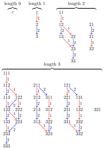
Figure 1. Part of the crystal graph for ${\smash{\mathrm{plac}}}_{3}$. Note that each connected component consists of words of the same length. In particular, the empty word $\varepsilon$ is an isolated vertex, and the words of length $1$ form a single connected component, which is the crystal basis for ${\smash{\mathrm{plac}}}_{3}$. The two connected components whose highest-weight words are $211$ and $121$ are isomorphic. However, the components consisting of the isolated vertex $321$ is not.

Since the operators $\tilde{e}_{i}$ and $\tilde{f}_{i}$ preserve lengths of words, and since there are finitely many words in $\mathcal{A}_{n}^{*}$ of each length, each connected component in the crystal graph must be finite.

For any $w\in\mathcal{A}_{n}^{*}$, let $\Gamma({\smash{\mathrm{plac}}}_{n},w)$ denote the connected component of $\Gamma({\smash{\mathrm{plac}}}_{n})$ that contains the vertex $w$. Notice that the crystal basis (3.3) is the connected component $\Gamma({\smash{\mathrm{plac}}}_{n},1)$.

A crystal isomorphism between two connected components is a weight-preserving labelled digraph isomorphism. That is, a map $\theta:\Gamma({\smash{\mathrm{plac}}}_{n},w)\to\Gamma({\smash{\mathrm{plac}}}_{n},w^{\prime})$ is a crystal isomorphism if it has the following properties:

• $\theta$ is bijective;

• $\mathrm{wt}\lparen\theta(u)\rparen=\mathrm{wt}\lparen u\rparen$ for all $u\in\Gamma({\smash{\mathrm{plac}}}_{n},w)$;

• for all $u,v\in\Gamma({\smash{\mathrm{plac}}}_{n},w)$, there is an edge if and only if there is an edge .

The possible definition (approach P3 in the introduction) of the relation $\equiv_{\smash{\mathrm{plac}}}$ using the crystal graph $\Gamma({\smash{\mathrm{plac}}}_{n})$ is the following: two words in $\mathcal{A}_{n}^{*}$ are related by $\equiv_{\smash{\mathrm{plac}}}$ if and only if they lie in the same place in isomorphic connected components. More formally, $w\equiv_{\smash{\mathrm{plac}}}w^{\prime}$ if and only if there is a crystal isomorphism $\theta:\Gamma({\smash{\mathrm{plac}}}_{n},w)\to\Gamma({\smash{\mathrm{plac}}}_{n},w^{\prime})$ such that $\theta(w)=w^{\prime}$ (see, for example, [Lec07]). For example, $2213\equiv_{\smash{\mathrm{plac}}}2231$, and these words appear in the same position in two of the connected components shown in Figure 2. (This figure also illustrates other properties that will be discussed shortly.)

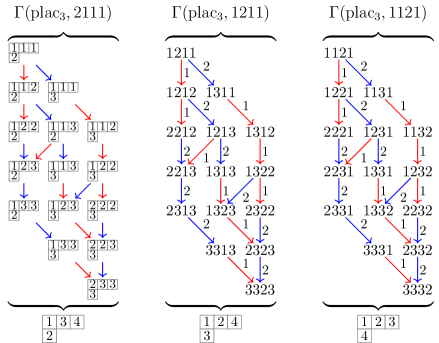
Figure 2. Three isomorphic components of the crystal graph for ${\smash{\mathrm{plac}}}_{3}$. In the component containing column readings of tableaux, the tableaux themselves are shown instead of words. The standard tableaux below each component is $\mathrm{Q}\lparen w\rparen$ for all words $w$ in that component.

3.3. Computing the Kashiwara operators

The recursive definition of the Kashiwara operators $\tilde{e}_{i}$ and $\tilde{f}_{i}$ given above is not particularly convenient for practical computation. The following method, outlined in [KN94], is more useful: Let $i\in\{1,\ldots,n-1\}$ and let $w\in\mathcal{A}_{n}^{*}$. Form a new word in $\{{+},{-}\}^{*}$ by replacing each letter $i$ of $w$ by the symbol $+$, each letter $i+1$ by the symbol $-$, and every other symbol with the empty word, keeping a record of the original letter replaced by each symbol. Then delete factors ${-}{+}$ until no such factors remain: the resulting word is ${+}^{\tilde{\phi}_{i}(w)}{-}^{\tilde{\epsilon}_{i}(w)}$, and is denoted by $\rho_{i}(w)$. Note that factors ${+}{-}$ are not deleted. (The method given in [KN94] involved deleting factors ${+}{-}$; again, this difference is a consequence of the choice of convention for reading tableaux.)

If $\tilde{\epsilon}_{i}(w)=0$, then $\tilde{e}_{i}(w)$ is undefined. If $\tilde{\epsilon}_{i}(w)>0$ then one obtains $\tilde{e}_{i}(w)$ by taking the letter $i+1$ which was replaced by the leftmost $-$ of $\rho_{i}(w)$ and changing it to $i$. If $\tilde{\phi}_{i}(w)=0$, then $\tilde{f}_{i}(w)$ is undefined. If $\tilde{\phi}_{i}(w)>0$ then one obtains $\tilde{f}_{i}(w)$ by taking the letter $i$ which was replaced by the rightmost $+$ of $\rho_{i}(w)$ and changing it to $i+1$.

For a purely combinatorial proof that this method of computation is correct, see [CGM, Proposition 2.1]. (Note that [CGM] uses the tableaux-reading convention from representation theory, so that the result must be reflected to fit the convention used here.)

3.4. Properties of the crystal graph

In the crystal graph $\Gamma({\smash{\mathrm{plac}}}_{n})$, the length of the longest path consisting of edges labelled by $i\in\{1,\ldots,n-1\}$ that ends at $w\in\mathcal{A}_{n}^{*}$ is $\tilde{\epsilon}_{i}(w)$. The length of the longest path consisting of edges labelled by $i$ that starts at $w\in\mathcal{A}_{n}^{*}$ is $\tilde{\phi}_{i}(w)$.

The operators $\tilde{e}_{i}$ and $\tilde{f}_{i}$ respectively increase and decrease weight whenever they are defined, in the sense that if $\tilde{e}_{i}(w)$ is defined, then $\mathrm{wt}\lparen\tilde{e}_{i}(w)\rparen>\mathrm{wt}\lparen w\rparen$, and if $\tilde{f}_{i}(w)$ is defined, then $\mathrm{wt}\lparen\tilde{f}_{i}(w)\rparen<\mathrm{wt}\lparen w\rparen$. This is because $\tilde{e}_{i}$ replaces a symbol $i+1$ with $i$ whenever it is defined, which corresponds to decrementing the $i+1$-th component and incrementing the $i$-th component of the weight, which results in an increase with respect to the order (2.1). Similarly, $\tilde{f}_{i}$ replaces a symbol $i$ with $i+1$ whenever it is defined. For this reason, the $\tilde{e}_{i}$ and $\tilde{f}_{i}$ are respectively known as the Kashiwara raising and lowering operators.

Every connected component in $\Gamma({\smash{\mathrm{plac}}}_{n})$ contains a unique highest-weight vertex: a vertex whose weight is higher than all other vertices in that component. This means that no Kashiwara raising operator $\tilde{e}_{i}$ is defined on this vertex. See [Shi05, § 2.4.2] for proofs and background. (The existence, but not the uniqueness, of a highest-weight vertex is a consequence of the finiteness of connected components.)

Whenever they are defined, the operators $\tilde{e}_{i}$ and $\tilde{f}_{i}$ preserve the property of being a tableau word and the shape of the corresponding tableau [KN94]. Furthermore, all the tableau words corresponding to tableaux of a given shape with entries in $\mathcal{A}_{n}$ lie in the same connected component. As shown in Figure 2, the left-hand component $\Gamma({\smash{\mathrm{plac}}}_{3},2111)$ is made up of all the tableau words corresponding to tableaux of shape $(3,1)$ with entries in $\mathcal{A}_{3}$.

Each connected component in $\Gamma({\smash{\mathrm{plac}}}_{n})$ corresponds to exactly one standard tableau, in the sense that $\mathrm{Q}\lparen w\rparen=\mathrm{Q}\lparen u\rparen$ if and only if $u$ and $w$ lies in the same connected component of $\Gamma({\smash{\mathrm{plac}}}_{n})$. In terms of the bijection $w\mapsto(\mathrm{P}\lparen w\rparen,\mathrm{Q}\lparen w\rparen)$ of the Robinson–Schensted–Knuth correspondence, specifying $\mathrm{Q}\lparen w\rparen$ locates the particular connected component $\Gamma({\smash{\mathrm{plac}}}_{n},w)$, and specifying $\mathrm{P}\lparen w\rparen$ locates the word $w$ within that component.

Highest-weight words in $\Gamma({\smash{\mathrm{plac}}}_{n})$, and in particular highest-weight tableau words, admit a useful characterization as Yamanouchi words. A word $w_{1}\cdots w_{m}\in\mathcal{A}_{n}^{*}$ (where $w_{i}\in\mathcal{A}_{n}$) is a Yamanouchi word if, for every $j=1,\ldots,m$, the weight of the suffix $w_{j}\cdots w_{m}$ is a non-increasing sequence (that is, a partition). Thus $1231$ is not a Yamanouchi word, since $\mathrm{wt}\lparen 31\rparen=(1,0,1)$, but $(1121$) is a Yamanouchi word, since $\mathrm{wt}\lparen 1121\rparen=(3,1,0)$; $\mathrm{wt}\lparen 121\rparen=(2,1,0)$; $\mathrm{wt}\lparen 21\rparen=(1,1,0)$, and $\mathrm{wt}\lparen 1\rparen=(1,0,0)$. A word is highest-weight if and only if it is a Yamanouchi word. See [Lot02, Ch. 5] for further background.

Highest-weight tableau words also have a neat characterization: a tableau word is highest-weight if and only if its weight is equal to the shape of the corresponding tableau. That is, a tableau word whose corresponding tableau has shape $\lambda$ is highest-weight if and only if, for each $i\in\mathcal{A}_{n}$, the number of symbols $i$ it contains is $\lambda_{i}$. It follows that a tableau whose reading is a highest-weight word must contain only symbols $i$ on its $i$-th row, for all $i\in\{1,\ldots,\ell\lparen\lambda\rparen\}$. For example, the tableau of shape $(5,3,2,2)$ whose reading is a highest-weight word is:

See [KN94] for further background.

4. Quasi-ribbon tableaux and insertion

This section gathers the relevant definitions and background on quasi-ribbon tableaux, the analogue of the Robinson–Schensted–Knuth correspondence, and the hypoplactic monoid. For further background, see [KT97, Nov00].

Let $\alpha=(\alpha_{1},\ldots,\alpha_{m})$ and $\beta=(\beta_{1},\ldots,\beta_{p})$ be compositions with $\lvert\alpha\rvert=\lvert\beta\rvert$. Then $\beta$ is coarser than $\alpha$, denoted $\beta\preceq\alpha$, if each partial sum $\beta_{1}+\ldots+\beta_{p^{\prime}}$ (for $p^{\prime}<p$) is equal to some partial sum $\alpha_{1}+\ldots+\alpha_{m^{\prime}}$ for some $m^{\prime}<m$. (Essentially, $\beta$ is coarser than $\alpha$ if it can be formed from $\alpha$ by ‘merging’ consecutive parts.) Thus $(11)\preceq(3,8)\preceq(3,6,2)\preceq(3,1,5,2)$.

A ribbon diagram of shape $\alpha$, where $\alpha$ is a composition, is an array of boxes, with $\alpha_{h}$ boxes in the $h$-th row, for $h=1,\ldots,\ell\lparen\alpha\rparen$ and counting rows from top to bottom, aligned so that the leftmost cell in each row is below the rightmost cell of the previous row. For example, the ribbon diagram of shape $(3,1,5,2)$ is:

(4.1)

Notice that a ribbon diagram cannot contain a $2\times 2$ subarray (that is, of the form ).

In a ribbon diagram of shape $\alpha$, the number of rows is $\ell\lparen\alpha\rparen$ and the number of boxes is $\lvert\alpha\rvert$.

A quasi-ribbon tableau of shape $\alpha$, where $\alpha$ is a composition, is a ribbon diagram of shape $\alpha$ filled with symbols from $\mathcal{A}$ such that the entries in every row are non-decreasing from left to right and the entries in every column are strictly increasing from top to bottom. An example of a quasi-ribbon tableau is

(4.2)

Note the following immediate consequences of the definition of a quasi-ribbon tableau: (1) for each $a\in\mathcal{A}$, the symbols $a$ in a quasi-ribbon tableau all appear in the same row, which must be the $j$-th row for some $j\leq a$; (2) the $h$-th row of a quasi-ribbon tableau cannot contain symbols from $\{1,\ldots,h-1\}$.

A quasi-ribbon tabloid is a ribbon diagram filled with symbols from $\mathcal{A}$ such that the entries in every column are strictly increasing from top to bottom. (Notice that there is no restriction on the order of entries in a row.) An example of a quasi-ribbon tabloid is

(4.3)

Note that a quasi-ribbon tableau is a special kind of quasi-ribbon tabloid.

A recording ribbon of shape $\alpha$, where $\alpha$ is a composition, is a ribbon diagram of shape $\alpha$ filled with symbols from $\{1,\ldots,\lvert\alpha\rvert\}$, with each symbol appearing exactly once, such that the entries in every row are increasing from left to right, and entries in every column are increasing from bottom to top. (Note that the condition on the order of entries in rows is the same as in quasi-ribbon tableau, but the condition on the order of entries in columns is the opposite of that in quasi-ribbon tableau.) An example of a recording ribbon of shape $(3,1,5,2)$ is

(4.4)

The column reading $\mathrm{C}\lparen T\rparen$ of a quasi-ribbon tabloid $T$ is the word in $\mathcal{A}^{*}$ obtained by proceeding through the columns, from leftmost to rightmost, and reading each column from bottom to top. For example, the column reading of the quasi-ribbon tableau (4.2) and the quasi-ribbon tabloid (4.3) are respectively $1\,2\,432\,4\,5\,5\,65\,7$ and $1\,5\,632\,2\,4\,5\,54\,7$ (where the spaces are simply for clarity, to show readings of individual columns), as illustrated below:

      

Let $w\in\mathcal{A}^{*}$, and let $w^{(1)}\cdots w^{(m)}$ be the factorization of $w$ into maximal decreasing factors. Let $\mathrm{QRoid}\lparen w\rparen$ be the quasi-ribbon tabloid whose $h$-th column has height $|w^{(h)}|$ and is filled with the symbols of $w^{(h)}$, for $h=1,\ldots,m$. (So each maximal decreasing factor of $w$ corresponds to a column of $\mathrm{QRoid}\lparen w\rparen$.) Then $\mathrm{C}\lparen\mathrm{QRoid}\lparen w\rparen\rparen=w$.

If $w$ is the column reading of some quasi-ribbon tableau $T$, it is called a quasi-ribbon word. It is easy to see that the word $w$ is a quasi-ribbon word if and only if $\mathrm{QRoid}\lparen w\rparen$ is a quasi-ribbon tableau. For example $433$ is not a quasi-ribbon word, since $\mathrm{QRoid}\lparen 433\rparen=\leavevmode\hbox to28.85pt{\vbox to29.25pt{\text{[drawing]}}}$ is the only quasi-ribbon tabloid whose column reading is $433$.

Proposition 4.1 ([Nov00, Proposition 3.4]).

A word $u\in\mathcal{A}^{*}$ is a quasi-ribbon word if and only if $\mathrm{std}\lparen u\rparen$ is a quasi-ribbon word.

The following algorithm gives a method for inserting a symbol into a quasi-ribbon tableau. It is due to Krob & Thibon, but is stated here in a slightly modified form:

Algorithm 4.2 ([KT97, § 7.2]).

Input: A quasi-ribbon tableau $T$ and a symbol $a\in\mathcal{A}$.

Output: A quasi-ribbon tableau $T\leftarrow a$.

Method: If there is no entry in $T$ that is less than or equal to $a$, output the quasi-ribbon tableau obtained by creating a new entry $a$ and attaching (by its top-left-most entry) the quasi-ribbon tableau $T$ to the bottom of $a$.

If there is no entry in $T$ that is greater than $a$, output the word obtained by creating a new entry $a$ and attaching (by its bottom-right-most entry) the quasi-ribbon tableau $T$ to the left of $a$.

Otherwise, let $x$ and $z$ be the adjacent entries of the quasi-ribbon tableau $T$ such that $x\leq a<z$. (Equivalently, let $x$ be the right-most and bottom-most entry of $T$ that is less than or equal to $a$, and let $z$ be the left-most and top-most entry that is greater than $a$. Note that $x$ and $z$ could be either horizontally or vertically adjacent.) Take the part of $T$ from the top left down to and including $x$, put a new entry $a$ to the right of $x$ and attach the remaining part of $T$ (from $z$ onwards to the bottom right) to the bottom of the new entry $a$, as illustrated here:

Output the resulting quasi-ribbon tableau.

Using an iterative form of this algorithm, one can start from a word $a_{1}\cdots a_{k}$ (where $a_{i}\in\mathcal{A}$) and compute a quasi-ribbon tableau $\mathrm{QR}\lparen a_{1}\cdots a_{k}\rparen$. Essentially, one simply starts with the empty quasi-ribbon tableau and inserts the symbols $a_{1}$, $a_{2}$, …, $a_{k}$ in order. However, the algorithm described below also computes a recording ribbon $\mathrm{RR}\lparen a_{1}\cdots a_{k}\rparen$, which will be used later in discussing an analogue of the Robinson–Schensted–Knuth correspondence.

Algorithm 4.3 ([KT97, § 7.2]).

Input: A word $a_{1}\cdots a_{k}$, where $a_{i}\in\mathcal{A}$.

Output: A quasi-ribbon tableau $\mathrm{QR}\lparen a_{1}\cdots a_{k}\rparen$ and a recording ribbon $\mathrm{RR}\lparen a_{1}\cdots a_{k}\rparen$.

Method: Start with the empty quasi-ribbon tableau $Q_{0}$ and an empty recording ribbon $R_{0}$. For each $i=1$, …, $k$, insert the symbol $a_{i}$ into $Q_{i-1}$ as per Algorithm 4.3; let $Q_{i}$ be the resulting quasi-ribbon tableau. Build the recording ribbon $R_{i}$, which has the same shape as $Q_{i}$, by adding an entry $i$ into $R_{i-1}$ at the same place as $a_{i}$ was inserted into $Q_{i-1}$.

Output $Q_{k}$ for $\mathrm{QR}\lparen a_{1}\cdots a_{k}\rparen$ and $R_{k}$ as $\mathrm{RR}\lparen a_{1}\cdots a_{k}\rparen$.

For example, the sequence of pairs $(Q_{i},R_{i})$ produced during the application of Algorithm 4.3 to the word $4323$ is

$$(\;,\;),\;\bigl{(}\leavevmode\hbox to14.63pt{\vbox to14.63pt{\text{[drawing]}}},\leavevmode\hbox to14.63pt{\vbox to14.63pt{\text{[drawing]}}}\bigr{)},\;\left(\leavevmode\hbox to14.63pt{\vbox to29.25pt{\text{[drawing]}}},\leavevmode\hbox to14.63pt{\vbox to29.25pt{\text{[drawing]}}}\right),\;\left(\leavevmode\hbox to14.63pt{\vbox to43.88pt{\text{[drawing]}}},\leavevmode\hbox to14.63pt{\vbox to43.88pt{\text{[drawing]}}}\right),\;\left(\leavevmode\hbox to28.85pt{\vbox to43.88pt{\text{[drawing]}}},\leavevmode\hbox to28.85pt{\vbox to43.88pt{\text{[drawing]}}}\right). {4} {1} {3} {4} {2} {1} {2} {3} {4} {3} {2} {1} {2} {3} {3} {4} {3} {2} {4} {1}$$

Therefore $\mathrm{QR}\lparen 4323\rparen=\leavevmode\hbox to28.85pt{\vbox to43.88pt{\text{[drawing]}}}$ and $\mathrm{RR}\lparen 4323\rparen=\leavevmode\hbox to28.85pt{\vbox to43.88pt{\text{[drawing]}}}$. It is straightforward to see that the map $u\mapsto(\mathrm{QR}\lparen u\rparen,\mathrm{RR}\lparen u)\rparen$ is a bijection between words in $\mathcal{A}^{*}$ and pairs consisting of a quasi-ribbon tableau and a recording ribbon [KT97, § 7.2] of the same shape; this is an analogue of the Robinson–Schensted–Knuth correspondence. For instace, if $\mathrm{QR}\lparen u\rparen$ is (4.2) and $\mathrm{RR}\lparen u\rparen$ is (4.4), then $u=12446553275$.

Recall the definition of $\mathcal{DC}\lparen\textvisiblespace\rparen$ from Subsection 2.2.

Proposition 4.4 ([Nov00, Theorems 4.12 & 4.16]).

For any word $u\in\mathcal{A}^{*}$, the shape of $\mathrm{QR}\lparen u\rparen$ (and of $\mathrm{RR}\lparen u\rparen$) is $\mathcal{DC}\lparen\mathrm{std}\lparen u\rparen^{-1}\rparen$.

The possible definition (approach H2 in the introduction) of the relation $\equiv_{\smash{\mathrm{hypo}}}$ using tableaux and insertion is the following:

$$u\equiv_{\smash{\mathrm{hypo}}}v\iff\mathrm{QR}\lparen u\rparen=\mathrm{QR}\lparen v\rparen.$$

Using this as a definition, it follows that $\equiv_{\smash{\mathrm{hypo}}}$ is a congruence on $\mathcal{A}^{*}$ [Nov00], which is known as the hypoplactic congruence on $\mathcal{A}^{*}$. The factor monoid $\mathcal{A}^{*}/{\equiv_{\smash{\mathrm{hypo}}}}$ is the hypoplactic monoid and is denoted ${\smash{\mathrm{hypo}}}$. The congruence $\equiv_{\smash{\mathrm{hypo}}}$ naturally restricts to a congruence on $\mathcal{A}_{n}^{*}$, and the factor monoid $\mathcal{A}_{n}^{*}/{\equiv_{\smash{\mathrm{hypo}}}}$ is the hypoplactic monoid of rank $n$ and is denoted ${\smash{\mathrm{hypo}}}_{n}$.

As noted above, if $w$ is a quasi-ribbon word, then $w=\mathrm{C}\lparen\mathrm{QR}\lparen w\rparen\rparen$. Thus the quasi-ribbon words in $\mathcal{A}^{*}$ form a cross-section (or set of normal forms) for ${\smash{\mathrm{hypo}}}$, and the quasi-ribbon words in $\mathcal{A}_{n}^{*}$ form a cross-section for ${\smash{\mathrm{hypo}}}_{n}$.

This paper also uses the following equivalent characterization of $\equiv_{\smash{\mathrm{hypo}}}$ [Nov00, Theorem 4.18]:

(4.5) $$u\equiv_{\smash{\mathrm{hypo}}}v\iff$$

$$\qquad\qquad\mathcal{DC}\lparen\mathrm{std}\lparen u\rparen^{-1}\rparen=\mathcal{DC}\lparen\mathrm{std}\lparen v\rparen^{-1}\rparen\land\mathrm{wt}\lparen u\rparen=\mathrm{wt}\lparen v\rparen.$$

5. Quasi-Kashiwara operators and the quasi-crystal graph

This section defines the quasi-Kashiwara operators and the quasi-crystal graph, and shows that isomorphisms between components of this graph give rise to a monoid. The following section will prove that this monoid is in fact the hypoplactic monoid.

Let $i\in\{1,\ldots,n-1\}$. Let $u\in\mathcal{A}_{n}^{*}$. The word $u$ has an $i$-inversion if it contains a symbol $i+1$ to the left of a symbol $i$. Equivalently, $u$ has an $i$-inversion if it contains a subsequence $(i+1)i$. (Recall from Subsection 2.1 that a subsequence may be made up of non-consecutive letters.) If the word $u$ does not have an $i$-inversion, it is said to be $i$-inversion-free.

Define the quasi-Kashiwara operators $\ddot{e}_{i}$ and $\ddot{f}_{i}$ on $\mathcal{A}_{n}^{*}$ as follows: Let $u\in\mathcal{A}_{n}^{*}$.

• If $u$ has an $i$-inverstion, both $\ddot{e}_{i}(u)$ and $\ddot{f}_{i}(u)$ are undefined.

• If $u$ is $i$-inversion-free, but $u$ contains at least one symbol $i+1$, then $\ddot{e}_{i}(u)$ is the word obtained from $u$ by replacing the left-most symbol $i+1$ by $i$; if $u$ contains no symbol $i+1$, then $\ddot{e}_{i}(u)$ is undefined.

• If $u$ is $i$-inversion-free, but $u$ contains at least one symbol $i$, then $\ddot{f}_{i}(u)$ is the word obtained from $u$ by replacing the right-most symbol $i$ by $i+1$; if $u$ contains no symbol $i$, then $\ddot{f}_{i}(u)$ is undefined.

For example,

$$\ddot{e}_{2}(3123) 3123 2$$ is undefined since has a -inversion;

$$\ddot{f}_{2}(3131) 3131 2$$ is undefined since is -inversion free

but does not contains a symbol $$2$$;

$$\ddot{f}_{1}(3113) =3123.$$

Define

$$\ddot{\epsilon}_{i}(u) =\max\big{\{}\,k\in\mathbb{N}\cup\{0\}:\text{$\underbrace{\ddot{e}_{i}\cdots\ddot{e}_{i}}_{\text{$k$ times}}(u)$ is defined}\,\big{\}};$$

$$\ddot{\phi}_{i}(u) =\max\big{\{}\,k\in\mathbb{N}\cup\{0\}:\text{$\underbrace{\ddot{f}_{i}\cdots\ddot{f}_{i}}_{\text{$k$ times}}(u)$ is defined}\,\big{\}}.$$

An immediate consequence of the definitions of $\ddot{e}_{i}$ and $\ddot{f}_{i}$ is that:

• If $u$ has an $i$-inverstion, then $\ddot{\epsilon}_{i}(u)=\ddot{\phi}_{i}(u)=0$;

• If $u$ is $i$-inversion-free, then every symbol $i$ lies to the left of every symbol $i+1$ in $u$, and so $\ddot{\epsilon}_{i}(u)=\lvert u\rvert_{i+1}$ and $\ddot{\phi}_{i}(u)=\lvert u\rvert_{i}$.

Remark 5.1.

It is worth noting how the quasi-Kashiwara operators $\ddot{e}_{i}$ and $\ddot{f}_{i}$ relate to the standard Kashiwara operators $\tilde{e}_{i}$ and $\tilde{f}_{i}$ as defined in Subsection 3.2. As discussed in Subsection 3.3, one computes the action of $\tilde{e}_{i}$ and $\tilde{f}_{i}$ on a word $u\in\mathcal{A}_{n}^{*}$ by replacing each symbol $i$ with $+$, each symbol $i+1$ with $-$, every other symbol with the empty word, and then iteratively deleting factors ${-}{+}$ until a word of the form ${+}^{p}{-}^{q}$ remains, whose left-most symbol ${-}$ and right-most symbol ${+}$ (if they exist) indicate the symbols in $u$ changed by $\tilde{e}_{i}$ and $\tilde{f}_{i}$ respectively. The deletion of factors ${-}{+}$ corresponds to rewriting to normal form a word representing an element of the bicyclic monoid $\langle\,{+},{-}\,|\,\mathopen{}({-}{+},\varepsilon)\,\rangle$. To compute the action of the quasi-Kashiwara operators $\ddot{e}_{i}$ and $\ddot{f}_{i}$ defined above on a word $u\in\mathcal{A}_{n}^{*}$, replace the symbols in the same way as before, but now rewrite to normal form as a word representing an element of the monoid $\langle\,{+},{-}\,|\,\mathopen{}({-}{+},0)\,\rangle$, where $0$ is a multiplicative zero. Any word that contains a symbol ${-}$ to the left of a symbol ${+}$ will be rewritten to $0$ and so $\ddot{e}_{i}$ and $\ddot{f}_{i}$ will be undefined in this case. If the word does not contain a symbol ${-}$ to the left of a symbol ${+}$, then it is of the form ${+}^{p}{-}^{q}$, and the left-most symbol $-$ and the right-most symbol $+$ indictate the symbols in $u$ changed by $\ddot{e}_{i}$ and $\ddot{f}_{i}$. In essence, one obtains the required analogies of the Kashiwara operators by replacing the bicyclic monoid $\langle\,{+},{-}\,|\,\mathopen{}({-}{+},\varepsilon)\,\rangle$, where ${-}{+}$ rewrites to the identity, with the monoid $\langle\,{+},{-}\,|\,\mathopen{}({-}{+},0)\,\rangle$, where ${-}{+}$ rewrites to the zero.

The action of the quasi-Kashiwara operators is essentially a restriction of the action of the Kashiwara operators:

Proposition 5.2.

Let $u\in\mathcal{A}_{n}^{*}$. If $\ddot{e}_{i}(u)$ is defined, so is $\tilde{e}_{i}(u)$, and $\tilde{e}_{i}(u)=\ddot{e}_{i}(u)$. If $\ddot{f}_{i}(u)$ is defined, so is $\tilde{f}_{i}(u)$, and $\tilde{f}_{i}(u)=\ddot{f}_{i}(u)$.

Proof.

Let $u\in\mathcal{A}_{n}^{*}$. Suppose the quasi-Kashiwara operator $\ddot{e}_{i}$ is defined on $u$. Then $u$ contains at least one symbol $i+1$ but is $i$-inversion-free, so that every symbol $i$ lies to the left of every symbol $i+1$ in $u$. So when one computes the action of $\tilde{e}_{i}$, replacing every symbol $i$ with the symbol ${+}$ and every symbol $i+1$ with the symbol ${-}$ leads immediately to the word ${+}^{\tilde{\phi}_{i}(u)}{-}^{\tilde{\epsilon}_{i}(u)}$ (that is, there are no factors ${-}{+}$ to delete). Hence $\tilde{\epsilon}_{i}(u)>0$, and so the Kashiwara operator $\tilde{e}_{i}$ is defined on $u$. Furthermore, $\tilde{e}_{i}$ acts by changing the symbol $i+1$ that contributed the leftmost ${-}$ to $i$, and, since there was no deletion of factors ${-}{+}$, this symbol must be the leftmost symbol $i+1$ in $u$. Thus $\tilde{e}_{i}(u)=\ddot{e}_{i}(u)$.

Similarly, if the quasi-Kashiwara operator $\ddot{f}_{i}$ is defined on $u$, so is the Kashiwara operator $\tilde{f}_{i}$, and $\tilde{f}_{i}(u)=\ddot{f}_{i}(u)$. ∎

The original definition of the Kashiwara operators $\tilde{e}_{i}$ and $\tilde{f}_{i}$ in Subsection 3.2 was recursive: whether the action on $uv$ recurses to the action on $u$ or on $v$ depends on the maximum number of times each operator can be applied to $u$ and $v$ separately. It seems difficult to give a similar recursive definition for the quasi-Kashiwara operators $\ddot{e}_{i}$ and $\ddot{f}_{i}$ defined here: if, for example, both operators can be applied zero times to $u$, this may mean that $u$ does not contain symbols $i$ or $i+1$, in which case the operators may still be defined on $uv$, or it may mean that $u$ contains a symbol $i+1$ to the left of a symbol $i$, in which case the operators are certainly not defined on $uv$.

This concludes the discussion contrasting the standard Kashiwara operators with the quasi-Kashiwara operators defined here. The aim now is to use the operators $\ddot{e}_{i}$ and $\ddot{f}_{i}$ to build the quasi-crystal graph and to establish some of its properties.

Lemma 5.3.

For all $i\in\{1,\ldots,n-1\}$, the operators $\ddot{e}_{i}$ and $\ddot{f}_{i}$ are mutually inverse, in the sense that if $\ddot{e}_{i}(u)$ is defined, $u=\ddot{f}_{i}(\ddot{e}_{i}(u))$, and if $\ddot{f}_{i}(u)$ is defined, $u=\ddot{e}_{i}(\ddot{f}_{i}(u))$.

Proof.

Let $u\in\mathcal{A}_{n}^{*}$. Suppose that $\ddot{e}_{i}(u)$ is defined. Then $u$ contains at least one symbol $i+1$ but is $i$-inversion-free, so that every symbol $i+1$ is to the right of every symbol $i$. Since $\ddot{e}_{i}(u)$ is obtained from $u$ by replacing the left-most symbol $i+1$ by $i$ (which becomes the right-most symbol $i$), every symbol $i+1$ is to the right of every symbol $i$ in the word $\ddot{e}_{i}(u)$ and so $\ddot{e}_{i}(u)$ is $i$-inversion-free, and $\ddot{e}_{i}(u)$ contains at least one symbol $i$. Thus $\ddot{f}_{i}(\ddot{e}_{i}(u))$ is defined, and is obtained from $\ddot{e}_{i}(u)$ by replacing the right-most symbol $i$ by $i+1$, which produces $u$. Hence if $\ddot{e}_{i}(u)$ is defined, $u=\ddot{f}_{i}(\ddot{e}_{i}(u))$. Similar reasoning shows that if $\ddot{f}_{i}(u)$ is defined, $u=\ddot{e}_{i}(\ddot{f}_{i}(u))$. ∎

The operators $\ddot{e}_{i}$ and $\ddot{f}_{i}$ respectively increase and decrease weight whenever they are defined, in the sense that if $\ddot{e}_{i}(u)$ is defined, then $\mathrm{wt}\lparen\ddot{e}_{i}(u)\rparen>\mathrm{wt}\lparen u\rparen$, and if $\ddot{f}_{i}(u)$ is defined, then $\mathrm{wt}\lparen\ddot{f}_{i}(u)\rparen<\mathrm{wt}\lparen u\rparen$. This is because $\ddot{e}_{i}$ replaces a symbol $i+1$ with $i$ whenever it is defined, which corresponds to decrementing the $i+1$-th component and incrementing the $i$-th component of the weight, which results in an increase with respect to the order (2.1). Similarly, $\ddot{f}_{i}$ replaces a symbol $i$ with $i+1$ whenever it is defined. For this reason, the $\ddot{e}_{i}$ and $\ddot{f}_{i}$ are respectively called the quasi-Kashiwara raising and lowering operators.

The quasi-crystal graph $\Gamma_{n}$ is the labelled directed graph with vertex set $\mathcal{A}_{n}^{*}$ and, for all $u\in\mathcal{A}_{n}^{*}$ and $i\in\{1,\ldots,n-1\}$, an edge from $u$ to $u^{\prime}$ labelled by $i$ if and only if $\ddot{f}_{i}(u)=u^{\prime}$ (or, equivalently by Lemma 5.3, $u=\ddot{e}_{i}(u^{\prime})$). Part of $\Gamma_{4}$ is shown in Figure 3. (The notation $\Gamma_{n}$ will be discarded in favour of $\Gamma({\smash{\mathrm{hypo}}}_{n})$ after it has been shown that the relationship between $\Gamma_{n}$ and ${\smash{\mathrm{hypo}}}_{n}$ is analogous to that between $\Gamma({\smash{\mathrm{plac}}}_{n})$ and ${\smash{\mathrm{plac}}}_{n}$.)

For any $u\in\mathcal{A}_{n}^{*}$, let $\Gamma_{n}(u)$ be the connected component of $\Gamma_{n}$ containing the vertex $u$. Notice that every vertex of $\Gamma_{n}$ has at most one incoming and at most one outgoing edge with a given label. A quasi-crystal isomorphism between two connected components is a weight-preserving labelled digraph isomorphism. (This parallels the definition of a crystal isomorphism in Subsection 3.2.)

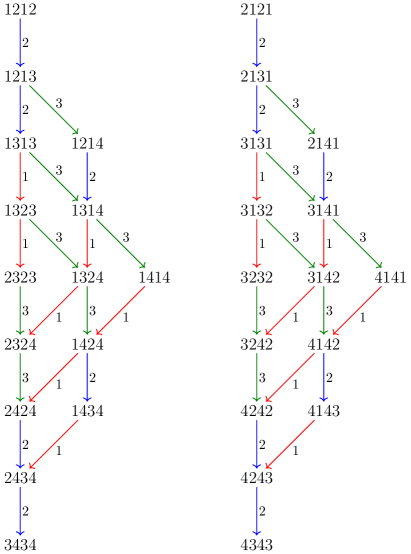
Figure 3. The isomorphic components $\Gamma_{4}(1212)$ and $\Gamma_{4}(2121)$ of the quasi-crystal graph $\Gamma_{4}$.

Define a relation $\sim$ on the free monoid $\mathcal{A}_{n}^{*}$ as follows: $u\sim v$ if and only if there is a quasi-crystal isomorphism $\theta:\Gamma_{n}(u)\to\Gamma_{n}(v)$ such that $\theta(u)=v$. That is, $u\sim v$ if and only if $u$ and $v$ are in the same position in isomorphic connected components of $\Gamma_{n}$. For example, $1324\sim 3142$, since these words are in the same position in their connected components, as can be seen in Figure 3.

The rest of this section is dedicated to proving that the relation $\sim$ is a congruence on $\mathcal{A}_{n}^{*}$. The proofs of this result and the necessary lemmata parallel the purely combinatorial proofs by the present authors and Gray [CGM, § 2.4] that isomorphisms of crystal graphs give rise to congruences.

Lemma 5.4.

Let $u,v,u^{\prime},v^{\prime}\in\mathcal{A}_{n}^{*}$. Suppose $u\sim v$ and $u^{\prime}\sim v^{\prime}$, and let $\theta:\Gamma_{n}(u)\to\Gamma_{n}(v)$ and $\theta^{\prime}:\Gamma_{n}(u^{\prime})\to\Gamma_{n}(v^{\prime})$ be quasi-crystal isomorphisms such that $\theta(u)=v$ and $\theta^{\prime}(u^{\prime})=v^{\prime}$. Let $i\in\{1,\ldots,n-1\}$. Then:

1. $\ddot{e}_{i}(uu^{\prime})$ is defined if and only if $\ddot{e}_{i}(vv^{\prime})$ is defined. If both are defined, exactly one of the following statements holds:

   1. $\ddot{e}_{i}(uu^{\prime})=u\ddot{e}_{i}(u^{\prime})$ and $\ddot{e}_{i}(vv^{\prime})=v\ddot{e}_{i}(v^{\prime})$;

   2. $\ddot{e}_{i}(uu^{\prime})=\ddot{e}_{i}(u)u^{\prime}$ and $\ddot{e}_{i}(vv^{\prime})=\ddot{e}_{i}(v)v^{\prime}$.

2. $\ddot{f}_{i}(uu^{\prime})$ is defined if and only if $\ddot{f}_{i}(vv^{\prime})$ is defined. If both are defined, exactly one of the following statements holds:

   1. $\ddot{f}_{i}(uu^{\prime})=u\ddot{f}_{i}(u^{\prime})$ and $\ddot{f}_{i}(vv^{\prime})=v\ddot{f}_{i}(v^{\prime})$;

   2. $\ddot{f}_{i}(uu^{\prime})=\ddot{f}_{i}(u)u^{\prime}$ and $\ddot{f}_{i}(vv^{\prime})=\ddot{f}_{i}(v)v^{\prime}$.

Proof.

Suppose $\ddot{e}_{i}(uu^{\prime})$ is defined. Then $uu^{\prime}$ is $i$-inversion-free, and contains at least one symbol $i+1$. Hence both $u$ and $u^{\prime}$ are $i$-inversion-free, and at least one of $u$ and $u^{\prime}$ contains a symbol $i+1$. Since $\theta$ and $\theta^{\prime}$ are crystal isomorphisms, $\mathrm{wt}\lparen u\rparen=\mathrm{wt}\lparen v\rparen$ and $\mathrm{wt}\lparen u^{\prime}\rparen=\mathrm{wt}\lparen v^{\prime}\rparen$ (and thus $u$ and $v$ contain the same number of each symbol, and $u^{\prime}$ and $v^{\prime}$ contain the same number of each symbol). Consider separately two cases depending on whether $u$ contains a symbol $i+1$:

• Suppose that $u$ does not contain a symbol $i+1$ (and hence $v$ does not contain a symbol $i+1$). Then $u^{\prime}$ must contain a symbol $i+1$ and indeed the left-most symbol $i+1$ of $uu^{\prime}$ must lie in $u^{\prime}$. So $\ddot{e}_{i}(u^{\prime})$ is defined and $\ddot{e}_{i}(uu^{\prime})=u\ddot{e}_{i}(u^{\prime})$. Thus there is an edge labelled by $i$ ending at $u^{\prime}$. Since $\theta^{\prime}$ is a quasi-crystal isomorphism, there is an edge labelled by $i$ ending at $v^{\prime}$. Hence $\ddot{e}_{i}(v^{\prime})$ is defined, and so $v^{\prime}$ is $i$-inversion-free. Since $v$ does not contain any symbol $i+1$, it follows that $vv^{\prime}$ is $i$-inversion-free. Hence $\ddot{e}_{i}(vv^{\prime})$ is defined and, since the left-most symbol $i+1$ of $vv^{\prime}$ lies in $v^{\prime}$, it also holds that $\ddot{e}_{i}(vv^{\prime})=v\ddot{e}_{i}(v^{\prime})$.

• Suppose that $u$ contains a symbol $i+1$ (and hence $v$ contains a symbol $i+1$). Then $u^{\prime}$ cannot contain a symbol $i$, and the left-most symbol $i+1$ of $uu^{\prime}$ must lie in $u$. Then $\ddot{e}_{i}(u)$ is defined and $\ddot{e}_{i}(uu^{\prime})=\ddot{e}_{i}(u)u^{\prime}$. So there is an edge labelled by $i$ ending at $u$. Since $\theta$ is a quasi-crystal isomorphism, there is an edge labelled by $i$ ending at $v$. Hence $\ddot{e}_{i}(v)$ is defined, and so $v$ is $i$-inversion-free. Since $v^{\prime}$ does not contain any symbol $i$, it follows that $vv^{\prime}$ is $i$-inversion-free. Hence $\ddot{e}_{i}(vv^{\prime})$ is defined and, since the left-most symbol $i+1$ in $vv^{\prime}$ lies in $v$, it also holds that $\ddot{e}_{i}(vv^{\prime})=\ddot{e}_{i}(v)v^{\prime}$.

This proves the forward implications of the three statements relating to $\ddot{e}_{i}$ in part (1). Interchanging $u$ and $u^{\prime}$ with $v$ and $v^{\prime}$ proves the reverse implications. The statements for $\ddot{f}_{i}$ in part (2) follow similarly. ∎

Lemma 5.5.

Let $u,v,u^{\prime},v^{\prime}\in\mathcal{A}_{n}^{*}$. Suppose $u\sim v$ and $u^{\prime}\sim v^{\prime}$, and let $\theta:\Gamma_{n}(u)\to\Gamma_{n}(v)$ and $\theta^{\prime}:\Gamma_{n}(u^{\prime})\to\Gamma_{n}(v^{\prime})$ be quasi-crystal isomorphisms such that $\theta(u)=v$ and $\theta^{\prime}(u^{\prime})=v^{\prime}$. Let $\ddot{g}_{i_{1}},\ldots,\ddot{g}_{i_{r}}\in\big{\{}\,\ddot{e}_{i},\ddot{f}_{i}:i\in\{1,\ldots,n-1\}\,\big{\}}$. Then:

1. $\ddot{g}_{i_{1}}\cdots\ddot{g}_{i_{r}}(uu^{\prime})$ is defined if and only if $\ddot{g}_{i_{1}}\cdots\ddot{g}_{i_{r}}(vv^{\prime})$ is defined.

2. When both $\ddot{g}_{i_{1}}\cdots\ddot{g}_{i_{r}}(uu^{\prime})$ and $\ddot{g}_{i_{1}}\cdots\ddot{g}_{i_{r}}(vv^{\prime})$ are defined, the sequence $\ddot{g}_{i_{1}},\ldots,\ddot{g}_{i_{r}}$ partitions into two subsequences $\ddot{g}_{j_{1}},\ldots,\ddot{g}_{j_{s}}$ and $\ddot{g}_{k_{1}},\ldots,\ddot{g}_{k_{t}}$ such that

   $$\ddot{g}_{i_{1}}\cdots\ddot{g}_{i_{r}}(uu^{\prime}) =\ddot{g}_{j_{1}}\cdots\ddot{g}_{j_{s}}(u)\ddot{g}_{k_{1}}\cdots\ddot{g}_{k_{t}}(u^{\prime}),$$

   $$\ddot{g}_{i_{1}}\cdots\ddot{g}_{i_{r}}(vv^{\prime}) =\ddot{g}_{j_{1}}\cdots\ddot{g}_{j_{s}}(v)\ddot{g}_{k_{1}}\cdots\ddot{g}_{k_{t}}(v^{\prime});$$

   where

   $$\theta\bigl{(}\ddot{g}_{j_{1}}\cdots\ddot{g}_{j_{s}}(u)\bigr{)} =\ddot{g}_{j_{1}}\cdots\ddot{g}_{j_{s}}(v),$$

   $$\theta^{\prime}\bigl{(}\ddot{g}_{k_{1}}\cdots\ddot{g}_{k_{t}}(u^{\prime})\bigr{)} =\ddot{g}_{k_{1}}\cdots\ddot{g}_{k_{t}}(v^{\prime}).$$

Proof.

This result follows by iterated application of Lemma 5.4, with the last two equalities holding because $\theta$ and $\theta^{\prime}$ are quasi-crystal isomorphisms with $\theta(u)=v$ and $\theta^{\prime}(u^{\prime})=v^{\prime}$. ∎

Proposition 5.6.

The relation $\sim$ is a congruence on the free monoid $\mathcal{A}_{n}^{*}$.

Proof.

It is clear from the definition that $\sim$ is an equivalence relation; it thus remains to prove that $\sim$ is compatible with multiplication in $\mathcal{A}_{n}^{*}$.

Suppose $u\sim v$ and $u^{\prime}\sim v^{\prime}$. Then there exist quasi-crystal isomorphisms $\theta:\Gamma_{n}(u)\to\Gamma_{n}(v)$ and $\theta:\Gamma_{n}(u^{\prime})\to\Gamma_{n}(v^{\prime})$ such that $\theta(u)=v$ and $\theta^{\prime}(u^{\prime})=v^{\prime}$.

Define a map $\Theta:\Gamma_{n}(uu^{\prime})\to\Gamma_{n}(vv^{\prime})$ as follows. For $w\in\Gamma_{n}(uu^{\prime})$, choose $\ddot{g}_{i_{1}},\ldots,\ddot{g}_{i_{r}}\in\big{\{}\,\ddot{e}_{i},\ddot{f}_{i}:i\in\{1,\ldots,n-1\}\,\big{\}}$ such that $\ddot{g}_{i_{1}}\cdots\ddot{g}_{i_{r}}(uu^{\prime})=w$; such a sequence exists because $w$ lies in the connected component $\Gamma_{n}(uu^{\prime})$. Define $\Theta(w)$ to be $\ddot{g}_{i_{1}}\cdots\ddot{g}_{i_{r}}(vv^{\prime})$; note that this is defined by Lemma 5.5(1).

It is necessary to prove that $\Theta$ is well-defined. Suppose that $\ddot{g}_{\hat{\imath}_{1}},\ldots,\ddot{g}_{\hat{\imath}_{m}}\in\big{\{}\,\ddot{e}_{i},\ddot{f}_{i}:i\in\{1,\ldots,n-1\}\,\big{\}}$ is such that $\ddot{g}_{\hat{\imath}_{1}}\cdots\ddot{g}_{\hat{\imath}_{m}}(uu^{\prime})=w$, and let $z=\ddot{g}_{\hat{\imath}_{1}}\cdots\ddot{g}_{\hat{\imath}_{m}}(vv^{\prime})$. Note that by Lemma 5.5(2),

• the sequence $\ddot{g}_{i_{1}},\ldots,\ddot{g}_{i_{r}}$ partitions into two subsequences $\ddot{g}_{j_{1}},\ldots,\ddot{g}_{j_{s}}$ and $\ddot{g}_{k_{1}},\ldots,\ddot{g}_{k_{t}}$ such that

  (5.1) $$\ddot{g}_{i_{1}}\cdots\ddot{g}_{i_{r}}(uu^{\prime})=\ddot{g}_{j_{1}}\cdots\ddot{g}_{j_{s}}(u)\ddot{g}_{k_{1}}\cdots\ddot{g}_{k_{t}}(u^{\prime});$$

• the sequence $\ddot{g}_{\hat{\imath}_{1}},\ldots,\ddot{g}_{\hat{\imath}_{m}}$ partitions into two subsequences $\ddot{g}_{\hat{\jmath}_{1}},\ldots,\ddot{g}_{\hat{\jmath}_{p}}$ and $\ddot{g}_{\hat{k}_{1}},\ldots,\ddot{g}_{\hat{k}_{q}}$ such that

  (5.2) $$\ddot{g}_{\hat{\imath}_{1}}\cdots\ddot{g}_{\hat{\imath}_{m}}(uu^{\prime})=\ddot{g}_{\hat{\jmath}_{1}}\cdots\ddot{g}_{\hat{\jmath}_{p}}(u)\ddot{g}_{\hat{k}_{1}}\cdots\ddot{g}_{\hat{k}_{q}}(u^{\prime}).$$

Since both $\ddot{g}_{i_{1}}\cdots\ddot{g}_{i_{r}}(uu^{\prime})$ and $\ddot{g}_{\hat{\imath}_{1}}\cdots\ddot{g}_{\hat{\imath}_{m}}(uu^{\prime})$ equal $w$, and since $\ddot{g}_{j_{1}}\cdots\ddot{g}_{j_{s}}(u)$ and $\ddot{g}_{\hat{\jmath}_{1}}\cdots\ddot{g}_{\hat{\jmath}_{p}}(u)$ have length $|u|$, it follows that

(5.3) $$\ddot{g}_{j_{1}}\cdots\ddot{g}_{j_{s}}(u) =\ddot{g}_{\hat{\jmath}_{1}}\cdots\ddot{g}_{\hat{\jmath}_{p}}(u);$$

$$\ddot{g}_{k_{1}}\cdots\ddot{g}_{k_{t}}(u^{\prime}) =\ddot{g}_{\hat{k}_{1}}\cdots\ddot{g}_{\hat{k}_{q}}(u^{\prime}).$$

Then

$$\Theta(w) =\ddot{g}_{i_{1}}\cdots\ddot{g}_{i_{r}}(vv^{\prime})$$ [by definition]

$$=\ddot{g}_{j_{1}}\cdots\ddot{g}_{j_{s}}(v)\ddot{g}_{k_{1}}\cdots\ddot{g}_{k_{t}}(v^{\prime})$$ [by (5.1)]

$$=\theta\bigl{(}\ddot{g}_{j_{1}}\cdots\ddot{g}_{j_{s}}(u)\bigr{)}\theta^{\prime}\bigl{(}\ddot{g}_{k_{1}}\cdots\ddot{g}_{k_{t}}(u^{\prime})\bigr{)}$$

$$=\theta\bigl{(}\ddot{g}_{\hat{\jmath}_{1}}\cdots\ddot{g}_{\hat{\jmath}_{p}}(u)\bigr{)}\theta^{\prime}\bigl{(}\ddot{g}_{\hat{k}_{1}}\cdots\ddot{g}_{\hat{k}_{q}}(u^{\prime})\bigr{)}$$ [by (5.3)]

$$=\ddot{g}_{\hat{\jmath}_{1}}\cdots\ddot{g}_{\hat{\jmath}_{p}}(v)\ddot{g}_{\hat{k}_{1}}\cdots\ddot{g}_{\hat{k}_{q}}(v^{\prime})$$

$$=\ddot{g}_{\hat{\imath}_{1}}\cdots\ddot{g}_{\hat{\imath}_{m}}(vv^{\prime})$$ [by (5.2)]

$$=z.$$

So $\Theta$ is well-defined.

By Lemma 5.5(1), $\Theta$ and its inverse preserve labelled edges. To see that $\Theta$ preserves weight, proceed as follows. Since $\theta$ and $\theta^{\prime}$ are quasi-crystal isomorphisms, $\mathrm{wt}\lparen u\rparen=\mathrm{wt}\lparen v\rparen$ and $\mathrm{wt}\lparen u^{\prime}\rparen=\mathrm{wt}\lparen v^{\prime}\rparen$. Hence $\mathrm{wt}\lparen uu^{\prime}\rparen=\mathrm{wt}\lparen vv^{\prime}\rparen$. Therefore if $\ddot{g}_{i_{1}}\cdots\ddot{g}_{i_{r}}(uu^{\prime})$ and $\ddot{g}_{i_{1}}\cdots\ddot{g}_{i_{r}}(vv^{\prime})$ are both defined, then both sequences of operators partition as above, and so

$$\mathrm{wt}\lparen w\rparen={} \mathrm{wt}\big{\lparen}\ddot{g}_{i_{1}}\cdots\ddot{g}_{i_{r}}(uu^{\prime})\big{\rparen}$$

$$={} \mathrm{wt}\big{\lparen}\ddot{g}_{j_{1}}\cdots\ddot{g}_{j_{s}}(u)\ddot{g}_{k_{1}}\cdots\ddot{g}_{k_{t}}(u^{\prime})\big{\rparen}$$

$$={} \mathrm{wt}\big{\lparen}\ddot{g}_{j_{1}}\cdots\ddot{g}_{j_{s}}(u)\big{\rparen}+\mathrm{wt}\big{\lparen}\ddot{g}_{k_{1}}\cdots\ddot{g}_{k_{t}}(u^{\prime})\big{\rparen}$$

$$={} \mathrm{wt}\big{\lparen}\theta(\ddot{g}_{j_{1}}\cdots\ddot{g}_{j_{s}}(u))\big{\rparen}+\mathrm{wt}\big{\lparen}\theta^{\prime}(\ddot{g}_{k_{1}}\cdots\ddot{g}_{k_{t}}(u^{\prime}))\big{\rparen}$$

[since $$\theta \theta^{\prime}$$ and preserve weights]

$$={} \mathrm{wt}\big{\lparen}\ddot{g}_{j_{1}}\cdots\ddot{g}_{j_{s}}(\theta(u))\big{\rparen}+\mathrm{wt}\big{\lparen}\ddot{g}_{k_{1}}\cdots\ddot{g}_{k_{t}}(\theta^{\prime}(u^{\prime}))\big{\rparen}$$

[since $$\theta \theta^{\prime}$$ and are quasi-crystal isomorphisms]

$$={} \mathrm{wt}\big{\lparen}\ddot{g}_{j_{1}}\cdots\ddot{g}_{j_{s}}(v)\big{\rparen}+\mathrm{wt}\big{\lparen}\ddot{g}_{k_{1}}\cdots\ddot{g}_{k_{t}}(v^{\prime})\big{\rparen}$$

$$={} \mathrm{wt}\big{\lparen}\ddot{g}_{j_{1}}\cdots\ddot{g}_{j_{s}}(v)\ddot{g}_{k_{1}}\cdots\ddot{g}_{k_{t}}(v^{\prime})\big{\rparen}$$

$$={} \mathrm{wt}\big{\lparen}\ddot{g}_{i_{1}}\cdots\ddot{g}_{i_{r}}(vv^{\prime})\big{\rparen}$$

$$={} \mathrm{wt}\lparen\Theta(w)\rparen.$$

Thus $\Theta$ is a quasi-crystal isomorphism. Hence $uu^{\prime}\sim vv^{\prime}$. Therefore the relation $\sim$ is a congruence. ∎

6. The quasi-crystal graph and the hypoplactic monoid

Since $\sim$ is a congruence, it makes sense to define the factor monoid $H_{n}=\mathcal{A}_{n}^{*}/{\sim}$. The aim is now to show that $H_{n}$ is the hypoplactic monoid ${\smash{\mathrm{hypo}}}_{n}$ by showing that $\sim$ is equal to the relation $\equiv_{\smash{\mathrm{hypo}}}$ on $\mathcal{A}_{n}^{*}$ as defined in Section 4 using quasi-ribbon tableaux and Algorithm 4.3. Some of the lemmata in this section are more complicated than necessary for this aim, because they will be used in future sections to prove other results.

Proposition 6.1.

Let $u\in\mathcal{A}_{n}^{*}$ and $i\in\{1,\ldots,n-1\}$.

1. If $\ddot{e}_{i}(u)$ is defined, then $\mathrm{std}\lparen\ddot{e}_{i}(u)\rparen=\mathrm{std}\lparen u\rparen$.

2. If $\ddot{f}_{i}(u)$ is defined, then $\mathrm{std}\lparen\ddot{f}_{i}(u)\rparen=\mathrm{std}\lparen u\rparen$.

Proof.

Suppose $\ddot{e}_{i}(u)$ is defined, and that $u$ contains $\sigma$ symbols $i$ and $\tau$ symbols $i+1$. Then during the computation of $\mathrm{std}\lparen u\rparen$, these symbols $i$ and $i+1$ become $i_{1},\ldots,i_{\sigma}$ and $(i+1)_{1},\ldots,(i+1)_{\tau}$ when subscripts are attached. Since $\ddot{e}_{i}(u)$ is defined, $u$ is $i$-inversion-free and so every symbol $i$ in $u$ is to the left of every symbol $i+1$, and $\ddot{e}_{i}(u)$ is obtained from $u$ by replacing the leftmost symbol $i+1$ by $i$. Thus, during the computation of $\mathrm{std}\lparen\ddot{e}_{i}(u)\rparen$, the symbols $i$ and $i+1$ become $i_{1},\ldots,i_{\sigma+1}$ and $(i+1)_{1},\ldots,(i+1)_{\tau-1}$. Thus, symbols $i_{1},\ldots,i_{\sigma},(i+1)_{1},\ldots,(i+1)_{\tau}$ and $i_{1},\ldots,i_{\sigma+1},(i+1)_{1},\ldots,(i+1)_{\tau-1}$ are replaced by the same symbols of the same rank in $\mathcal{A}$. Hence $\mathrm{std}\lparen\ddot{e}_{i}(u)\rparen=\mathrm{std}\lparen u\rparen$. This proves part (1); similar reasoning proves part (2). ∎

Corollary 6.2.

If $u\in\mathcal{A}_{n}^{*}$ is a quasi-ribbon word, then every word in $\Gamma_{n}(u)$ is quasi-ribbon word, and all of the corresponding quasi-ribbon tableaux have the same shape as $\mathrm{QR}\lparen u\rparen$.

Proof.

Let $w\in\Gamma_{n}(u)$. By Proposition 6.1, $\mathrm{std}\lparen w\rparen=\mathrm{std}\lparen u\rparen$. Thus by Proposition 4.1, $w$ is a quasi-ribbon word, and by Proposition 4.4, $\mathrm{QR}\lparen w\rparen$ has the same shape as $\mathrm{QR}\lparen u\rparen$. ∎

Lemma 6.3.

Let $i\in\{1,\ldots,n-1\}$. Let $u\in\mathcal{A}_{n}^{*}$ be a quasi-ribbon word. Then:

1. $\ddot{e}_{i}(u)$ is defined if and only if $\mathrm{QR}\lparen u\rparen$ contains some symbol $i+1$ but does not contain $i+1$ below $i$ in the same column;

2. $\ddot{f}_{i}(u)$ is defined if and only if $\mathrm{QR}\lparen u\rparen$ contains some symbol $i$ but does not contain $i+1$ below $i$ in the same column.

Proof.

By the definition of the reading of a quasi-ribbon tableau, and the fact that the rows of quasi-ribbon tableaux are non-decreasing from left to right, the word $u$ has an $i$-inversion if and only if $i+1$ and $i$ appear in the same column of $\mathrm{QR}\lparen u\rparen$. Thus part (1) follows immediately from the definition of $\ddot{e}_{i}$. Part (2) follows by similar reasoning for $\ddot{f}_{i}$. ∎

Proposition 6.4.

Let $\alpha$ be a composition.

1. The set of quasi-ribbon words corresponding to quasi-ribbon tableaux of shape $\alpha$ forms a single connected component of $\Gamma_{n}$.

2. In this connected component, there is a unique highest-weight word, which corresponds to the quasi-ribbon tableau of shape $\alpha$ whose $j$-th row consists entirely of symbols $j$, for $j=1,\ldots,\ell\lparen\alpha\rparen$.

Proof.

Let $w$ be the quasi-ribbon word such that $\mathrm{QR}\lparen w\rparen$ has shape $\alpha$ and has $j$-th row full of symbols $j$, for each $j=1,\ldots,\ell\lparen\alpha\rparen$. Clearly $\ddot{e}_{i}(w)$ cannot be defined for any $i\geq\ell\lparen\alpha\rparen$, since there are no symbols $i+1$ in the word $w$. Furthermore, for $i=1,\ldots,\ell\lparen\alpha\rparen-1$, the right-most entry $i$ in the $i$-th row of $T$ lies immediately above the left-most entry $i+1$ in the $i+1$-th row. Thus, by Lemma 6.3, $\ddot{e}_{i}(w)$ is not defined. Hence $w$ is highest-weight. (Note that it is still necessary to show that $w$ is the unique highest-weight word in its connected component of $\Gamma_{n}$.)

Let $u$ be a quasi-ribbon word such that $\mathrm{QR}\lparen u\rparen$ has shape $\alpha$ but has the property that the $j$-th row does not consist entirely of symbols $j$, for at least one $j\in\{1,\ldots,\ell\lparen\alpha\rparen\}$. Thus there is some symbol $i$ that appears in the $h$-th row, where $h<i$. Without loss of generality, assume $i$ is minimal. Clearly $i>1$ since $h\geq 1$. Consider two cases:

• The left-most symbol in the $h$-th row is $i$. Then, by the minimality of $i$, the symbol $i-1$ cannot appear in $u$, for it would have to appear on the $h-1$-row of $\mathrm{QR}\lparen u\rparen$. Thus $u$ does not contain a symbol $i-1$; hence $\ddot{e}_{i-1}(u)$ is defined.

• The left-most symbol in the $h$-th row is not $i$. Then every symbol $i-1$ in $\mathrm{QR}\lparen u\rparen$ must appear in a column strictly to the left of the left-most symbol $i$. Hence, by Lemma 6.3, $\ddot{e}_{i-1}(u)$ is defined.

Thus some quasi-Kashiwara operator $\ddot{e}_{i}$ can be applied to $u$ and so $u$ is not a highest-weight word.

This implies that $w$ is the unique highest-weight quasi-ribbon word that has shape $\alpha$. Furthermore, by Corollary 6.2, applying $\ddot{e}_{i}$ raises the weight of a word but maintains the property of being a quasi-ribbon word and the shape $\alpha$ of its corresponding quasi-ribbon tableau. Therefore some sequence of operators $\ddot{e}_{i}$ must transform the word $u$ to the word $w$. Thus the set of quasi-ribbon words whose corresponding quasi-ribbon tableau have shape $\alpha$ forms a connected component. ∎

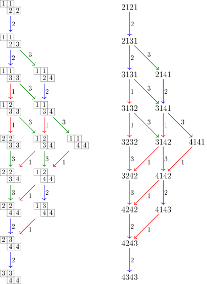
Figure 4. The isomorphic components $\Gamma_{4}(1212)$ (left) and $\Gamma_{4}(2121)$ (right) of the quasi-crystal graph $\Gamma_{4}$, with elements of $\Gamma_{4}(1212)$ drawn as quasi-ribbon tableau instead of written as words. The component $\Gamma_{4}(1212)$ consists of all quasi-ribbon words whose quasi-ribbon tableaux have shape $(2,2)$. None of the words in $\Gamma_{4}(2112)$ is a quasi-ribbon word.

Thus, for example, the highest-weight quasi-ribbon word corresponding to a quasi-ribbon tableau of shape $(3,1,5,2)$ is $11321333434$, corresponding to the quasi-ribbon tableau

See also Figures 3 and 4, where the connected component $\Gamma_{4}(1212)$, shown on the left, consists entirely of quasi-ribbon words corresponding to quasi-ribbon tableaux of shape $(2,2)$, and its unique highest-weight word is $1212$.

Note that Proposition 6.4(2) only establishes the existence of unique highest-weight words in connected components consisting of quasi-ribbon words, and not in every component.

Corollary 6.5.

Let $\alpha$ be a composition, and let $w$ be a quasi-ribbon word such that $\mathrm{QR}\lparen w\rparen$ has shape $\alpha$. Then $w$ is a highest-weight word if and only if $\mathrm{wt}\lparen w\rparen=\alpha$.

Proof.

Suppose $w$ is a highest-weight word. By Proposition 6.4(2), the $j$-th row of $\mathrm{QR}\lparen w\rparen$ consists entirely of symbols $j$, for $j=1,\ldots,\ell\lparen\alpha\rparen$. Thus $w$ contains exactly $\alpha_{j}$ symbols $j$ for each $j$, and so $\mathrm{wt}\lparen w\rparen=\alpha$.

Now suppose that $\mathrm{wt}\lparen w\rparen=\alpha$. In a quasi-ribbon tableau, a symbol $j$ can only appear in rows $1$ to $j$. Hence the $\alpha_{1}$ symbols $1$ in $\mathrm{QR}\lparen w\rparen$ must appear in row $1$, which has length $\alpha_{1}$, so this row is full of symbols $1$. The $\alpha_{2}$ symbols $2$ must appear in rows $1$ and $2$, but row $1$ is full of symbols $1$, so row $2$, which has length $\alpha_{2}$, is full of symbols $2$. Continuing in this way, row $j$, which has length $\alpha_{j}$, is full of symbols $j$. By Proposition 6.4(2), $w$ is a highest-weight word. ∎

Corollary 6.6.

Let $u,v\in\mathcal{A}_{n}^{*}$ be highest-weight quasi-ribbon words. If $\mathrm{wt}\lparen u\rparen=\mathrm{wt}\lparen v\rparen$, then $u=v$.

Proof.

By Corollary 6.5, since $u$ and $v$ are highest-weight, $\mathrm{QR}\lparen u\rparen$ has shape $\mathrm{wt}\lparen u\rparen$ and $\mathrm{QR}\lparen v\rparen$ has shape $\mathrm{wt}\lparen v\rparen$. Since these weights are equal, $\mathrm{QR}\lparen u\rparen$ and $\mathrm{QR}\lparen v\rparen$ have the same shape. By the characterization of highest-weight words in Proposition 6.4(2), it follows that $u=v$. ∎

Proposition 6.7.

There is at most one quasi-ribbon word in each $\sim$-class.

Proof.

Suppose $u,v\in\mathcal{A}_{n}^{*}$ are quasi-ribbon words with $u\sim v$. By Proposition 6.4, there is a sequence of operators $\ddot{e}_{i_{1}},\ldots,\ddot{e}_{i_{k}}$ such that $u^{\prime}=\ddot{e}_{i_{1}}\cdots\ddot{e}_{i_{k}}(u)$ is highest-weight. Since $u\sim v$ implies that the words $u$ and $v$ are at the same location in the isomorphic components $\Gamma_{n}(u)$ and $\Gamma_{n}(v)$, the word $v^{\prime}=\ddot{e}_{i_{1}}\cdots\ddot{e}_{i_{k}}(v)$ is also highest-weight. The isomorphism from $\Gamma_{n}(u)$ to $\Gamma_{n}(v)$ preserves weight, and so $\mathrm{wt}\lparen u\rparen=\mathrm{wt}\lparen v\rparen$. Thus $u=v$ by Corollary 6.6. ∎

Proposition 6.7 shows that each element of $H_{n}=\mathcal{A}_{n}^{*}/{\sim}$ has at most one representative as a quasi-ribbon word. The aim is now to show that if two words are $\equiv_{\smash{\mathrm{hypo}}}$-related, then they are $\sim$-related, which will establish a one-to-one correspondence between the elements of $H_{n}$ and quasi-ribbon tableaux:

Lemma 6.8.

Let $u\in\mathcal{A}_{n}^{*}$. Then $u$ and $\mathrm{C}\lparen\mathrm{QR}\lparen u\rparen\rparen$ have exactly the same labelled edges incident to them in $\Gamma_{n}$.

Proof.

The aim is to prove that $\ddot{e}_{i}(u)$ is defined if and only if $\ddot{e}_{i}(\mathrm{C}\lparen\mathrm{QR}\lparen u\rparen\rparen)$ is defined. Similar reasoning shows that $\ddot{f}_{i}(u)$ is defined if and only if $\ddot{f}_{i}(\mathrm{C}\lparen\mathrm{QR}\lparen u\rparen\rparen)$ is defined.

First, note that since $u\equiv_{\smash{\mathrm{hypo}}}\mathrm{C}\lparen\mathrm{QR}\lparen u\rparen\rparen$, it follows from (4.5) that $\mathrm{wt}\lparen u\rparen=\mathrm{wt}\lparen\mathrm{C}\lparen\mathrm{QR}\lparen u\rparen\rparen\rparen$. Suppose $\ddot{e}_{i}(u)$ is defined. Then $u$ contains a symbol $i+1$ but is $i$-inversion-free. Hence every symbol $i$ is to the left of every symbol $i+1$ in $u$. Therefore Algorithm 4.3 appends the symbols $i+1$ to the right of any symbols $i$. Hence by Lemma 6.3, $\ddot{e}_{i}(\mathrm{C}\lparen\mathrm{QR}\lparen u\rparen\rparen)$ is defined. On the other hand, suppose that $\ddot{e}_{i}(\mathrm{C}\lparen\mathrm{QR}\lparen u\rparen\rparen)$ is defined. Then by Lemma 6.3, $\mathrm{C}\lparen\mathrm{QR}\lparen u\rparen\rparen$ contains a symbol $i+1$, but no symbol $i$ immediately above $i+1$ in a column. Hence the computation of $\mathrm{QR}\lparen u\rparen$ using Algorithm 4.3 cannot involve inserting a symbol $i$ later than a symbol $i+1$. That is, $u$ is $i$-inversion-free. Since $\mathrm{QR}\lparen u\rparen$ contains a symbol $i+1$, so does $u$, and thus $\ddot{e}_{i}(u)$ is defined. ∎

Lemma 6.9.

Let $u\in\mathcal{A}_{n}^{*}$ and $i\in\{1,\ldots,n-1\}$.

1. Suppose that $\ddot{e}_{i}(u)$ is defined. Then $\ddot{e}_{i}(u)\equiv_{\smash{\mathrm{hypo}}}\ddot{e}_{i}(\mathrm{C}\lparen\mathrm{QR}\lparen u\rparen\rparen)$ and so $\ddot{e}_{i}(\mathrm{C}\lparen\mathrm{QR}\lparen u\rparen\rparen)=\mathrm{C}\lparen\mathrm{QR}\lparen\ddot{e}_{i}(u)\rparen\rparen$.

2. Suppose that $\ddot{f}_{i}(u)$ is defined. Then $\ddot{f}_{i}(u)\equiv_{\smash{\mathrm{hypo}}}\ddot{f}_{i}(\mathrm{C}\lparen\mathrm{QR}\lparen u\rparen\rparen)$ and so $\ddot{f}_{i}(\mathrm{C}\lparen\mathrm{QR}\lparen u\rparen\rparen)=\mathrm{C}\lparen\mathrm{QR}\lparen\ddot{f}_{i}(u)\rparen\rparen$.

Proof.

Suppose that $\ddot{e}_{i}(u)$ is defined. Then it follows from Lemma 6.8 that $\ddot{e}_{i}(\mathrm{C}\lparen\mathrm{QR}\lparen u\rparen\rparen)$ is also defined. Now, $u\equiv_{\smash{\mathrm{hypo}}}\mathrm{C}\lparen\mathrm{QR}\lparen u\rparen\rparen$ by the definition of $\equiv_{\smash{\mathrm{hypo}}}$. Thus it follows from (4.5) that $\mathrm{wt}\lparen u\rparen=\mathrm{wt}\lparen\mathrm{C}\lparen\mathrm{QR}\lparen u\rparen\rparen\rparen$ and so $\mathrm{wt}\lparen\ddot{e}_{i}(u)\rparen=\mathrm{wt}\lparen\ddot{e}_{i}(\mathrm{C}\lparen\mathrm{QR}\lparen u\rparen\rparen)\rparen$ since $\ddot{e}_{i}$ replaces one symbol $i+1$ by a symbol $i$ in both words. Further, it again follows from (4.5) that $\mathcal{DC}\lparen\mathrm{std}\lparen u\rparen^{-1}\rparen=\mathcal{DC}\lparen\mathrm{std}\lparen\mathrm{C}\lparen\mathrm{QR}\lparen u\rparen\rparen\rparen^{-1}\rparen$. Hence, since $\ddot{e}_{i}$ preserves standardizations by Proposition 6.1, it follows that $\mathcal{DC}\lparen\mathrm{std}\lparen\ddot{e}_{i}(u)\rparen^{-1}\rparen=\mathcal{DC}\lparen\mathrm{std}\lparen\ddot{e}_{i}(\mathrm{C}\lparen\mathrm{QR}\lparen u\rparen\rparen)\rparen^{-1}\rparen$. Combining this with the equality of weights and using (4.5) again shows that $\ddot{e}_{i}(u)\equiv_{\smash{\mathrm{hypo}}}\ddot{e}_{i}(\mathrm{C}\lparen\mathrm{QR}\lparen u\rparen\rparen)$.

By Corollary 6.2, $\ddot{e}_{i}(\mathrm{C}\lparen\mathrm{QR}\lparen u\rparen\rparen)$ is a quasi-ribbon word. Since it is $\equiv_{\smash{\mathrm{hypo}}}$-related to $\ddot{e}_{i}(u)$, it follows that $\ddot{e}_{i}(\mathrm{C}\lparen\mathrm{QR}\lparen u\rparen\rparen)=\mathrm{C}\lparen\mathrm{QR}\lparen\ddot{e}_{i}(u)\rparen\rparen$. This completes the proof of part (1); similar reasoning proves part (2). ∎

Proposition 6.10.

Let $u,v\in\mathcal{A}_{n}^{*}$. Then $u\equiv_{\smash{\mathrm{hypo}}}v\implies u\sim v$.

Proof.

By Lemmata 6.8 and 6.9, the map $\Theta:\Gamma_{n}(u)\to\Gamma_{n}(\mathrm{C}\lparen\mathrm{QR}\lparen u\rparen\rparen)$ with $\Theta(w)=\mathrm{C}\lparen\mathrm{QR}\lparen w\rparen\rparen$ (for $w\in\Gamma_{n}(u)$) is a quasi-crystal isomorphism, and so $u\sim\mathrm{C}\lparen\mathrm{QR}\lparen u\rparen\rparen$. Similarly, $v\sim\mathrm{C}\lparen\mathrm{QR}\lparen v\rparen\rparen$. It follows from $u\equiv_{\smash{\mathrm{hypo}}}v$ that $\mathrm{QR}\lparen u\rparen=\mathrm{QR}\lparen v\rparen$. Since $\sim$ is transitive, $u\sim v$. ∎

Let $u\in\mathcal{A}_{n}^{*}$. By Proposition 6.10, $\mathrm{QR}\lparen u\rparen$ is a quasi-ribbon word that is $\sim$-related to $u$. By Proposition 6.7, $\mathrm{QR}\lparen u\rparen$ is the unique quasi-ribbon word that is $\sim$-related to $u$. Thus the following result has been proven:

Theorem 6.11.

Let $u,v\in\mathcal{A}_{n}^{*}$. Then $u\equiv_{\smash{\mathrm{hypo}}}v\iff u\sim v$.

Corollary 6.12.

${\smash{\mathrm{hypo}}}_{n}=\mathcal{A}_{n}^{*}/{\equiv_{\smash{\mathrm{hypo}}}}\simeq\mathcal{A}_{n}^{*}/{\sim}=H_{n}$.

In light of this, henceforth the quasi-crystal graph $\Gamma_{n}$ is denoted $\Gamma({\smash{\mathrm{hypo}}}_{n})$, and the connected component $\Gamma_{n}(w)$ is denoted $\Gamma({\smash{\mathrm{hypo}}}_{n},w)$

Before moving on to study how the quasi-crystal graph interacts with the hypoplactic version of the Robinson–Schensted–Knuth correspondence, it is necessary to prove one more fundamental property of the quasi-crystal graph. Proposition 6.4(2) showed that the connected components comprising quasi-ribbon words contain unique highest-weight words. The same holds for all connected components:

Proposition 6.13.

In every connected component in $\Gamma({\smash{\mathrm{hypo}}}_{n})$ there is a unique highest-weight word.

Proof.

Let $u\in\mathcal{A}_{n}^{*}$. Since $u\sim\mathrm{C}\lparen\mathrm{QR}\lparen u\rparen\rparen$, the connected component $\Gamma({\smash{\mathrm{hypo}}}_{n},u)$ is isomorphic to $\Gamma({\smash{\mathrm{hypo}}}_{n},\mathrm{C}\lparen\mathrm{QR}\lparen u\rparen\rparen)$. By Proposition 6.4(2), there is a unique highest-weight word in $\Gamma({\smash{\mathrm{hypo}}}_{n},\mathrm{C}\lparen\mathrm{QR}\lparen u\rparen\rparen)$. Consequently, $\Gamma({\smash{\mathrm{hypo}}}_{n},u)$ contains a unique highest-weight word. ∎

In the crystal graph of the plactic monoid (that is the plactic monoid of type $A_{n}$), the highest-weight words are characterized combinatorially as follows. Recall from Subsection 3.4 that a Yamanouchi word is a word $w$ in $\mathcal{A}_{n}^{*}$ such for any suffix $v$ of $w$, it holds that $|v|_{1}\geq|v|_{2}\geq\ldots\geq|v|_{n}$. The highest-weight words in the crystal graph of the plactic monoid are precisely the Yamanouchi words [Lot02, § 5.5].

Yamanouchi words do not characterize highest-weight words in connected components of the quasi-crystal graph $\Gamma({\smash{\mathrm{hypo}}}_{n})$. For example, the highest-weight word in $\Gamma({\smash{\mathrm{hypo}}}_{n},2112)$ is $2112$, which has the suffix $v=2$ that does not satisfy $|v|_{1}\geq|v|_{2}$.

Let $\max(u)$ denote the largest symbol in the word $u$.

Proposition 6.14.

A word $u\in\mathcal{A}_{n}^{*}$ is highest-weight in a component of $\Gamma({\smash{\mathrm{hypo}}}_{n})$ if and only if it contains all symbols in $\{1,\ldots,\max(u)\}$, with the condition that it has an $i$-inversion for all $i\in\{1,\ldots,\max(u)-1\}$.

Proof.

These are precisely the words for which all operators $\ddot{e}_{i}$ are undefined. ∎

In the crystal graph $\Gamma({\smash{\mathrm{plac}}}_{n})$, suffixes of highest-weight words are also highest-weight; this is an immediate consequence of the definition of a Yamanouchi word. This does not hold in $\Gamma({\smash{\mathrm{hypo}}}_{n})$: the highest-weight word $2112$ has the suffix $2$, which is not highest-weight.

7. The quasi-crystal graph and the Robinson–Schensted–Knuth correspondence

The previous sections constructed the quasi-crystal graph $\Gamma({\smash{\mathrm{hypo}}}_{n})$ and showed that the hypoplactic congruence $\equiv_{\smash{\mathrm{hypo}}}$ corresponds to quasi-crystal isomorphisms (that is, weight-preserving labelled digraph isomorphisms) between its connected components, just as the plactic congruence $\equiv_{\smash{\mathrm{plac}}}$ corresponds to crystal isomorphisms (that is, weight-preserving labelled digraph isomorphisms) between connected components of the crystal graph $\Gamma({\smash{\mathrm{plac}}}_{n})$. The following result shows that the interaction of the quasi-crystal graph and the hypoplactic analogue of the Robinson–Schensted–Knuth correspondence exactly parallels the very elegant interaction of the crystal graph and the usual Robinson–Schensted–Knuth correspondence. Just as the connected components of the crystal graph $\Gamma({\smash{\mathrm{plac}}}_{n})$ are indexed by standard Young tableaux, the connected components of the quasi-crystal graph $\Gamma({\smash{\mathrm{hypo}}}_{n})$ are indexed by recording ribbons:

Theorem 7.1.

Let $u,v\in\mathcal{A}_{n}^{*}$. The words $u$ and $v$ lie in the same connected component of $\Gamma({\smash{\mathrm{hypo}}}_{n})$ if and only if $\mathrm{RR}\lparen u\rparen=\mathrm{RR}\lparen v\rparen$.

Proof.

Suppose that $u$ and $v$ lie in the same connected component of $\Gamma({\smash{\mathrm{hypo}}}_{n})$. Note first that $|u|=|v|$. Let $u=u_{1}\cdots u_{k}$ and $v=v_{1}\cdots v_{k}$, where $u_{h},v_{h}\in\mathcal{A}_{n}$. By Proposition 6.1, $\mathrm{std}\lparen u\rparen=\mathrm{std}\lparen v\rparen$. Therefore $\mathrm{std}\lparen u_{1}\cdots u_{h}\rparen=\mathrm{std}\lparen v_{1}\cdots v_{h}\rparen$ for all $h$ (this is immediate from the definition of standardization [Nov00, Lemma 2.2]). Thus $\mathrm{QR}\lparen u_{1}\cdots u_{h}\rparen$ and $\mathrm{QR}\lparen v_{1}\cdots v_{h}\rparen$ both have shape $\mathcal{DC}\lparen\mathrm{std}\lparen u_{1}\cdots u_{h}\rparen^{-1}\rparen$ for all $h$. The sequence of these shapes determines where new symbols are inserted during the computation of $\mathrm{QR}\lparen u\rparen$ and $\mathrm{QR}\lparen v\rparen$ by Algorithm 4.3, and so $\mathrm{RR}\lparen u\rparen=\mathrm{RR}\lparen v\rparen$.

Now suppose $\mathrm{RR}\lparen u\rparen=\mathrm{RR}\lparen v\rparen$. Let $\hat{u}$ and $\hat{v}$ be the highest-weight words in $\Gamma({\smash{\mathrm{hypo}}}_{n},u)$ and $\Gamma({\smash{\mathrm{hypo}}}_{n},v)$, respectively. By the forward implications, $\mathrm{RR}\lparen\hat{u}\rparen=\mathrm{RR}\lparen u\rparen=\mathrm{RR}\lparen v\rparen=\mathrm{RR}\lparen\hat{v}\rparen$. Note that $\hat{u}\sim\mathrm{C}\lparen\mathrm{QR}\lparen\hat{u}\rparen\rparen$ and $\hat{v}\sim\mathrm{C}\lparen\mathrm{QR}\lparen\hat{v}\rparen\rparen$, and $\mathrm{C}\lparen\mathrm{QR}\lparen\hat{u}\rparen\rparen$ and $\mathrm{C}\lparen\mathrm{QR}\lparen\hat{v}\rparen\rparen$ are highest-weight quasi-ribbon words. Furthermore, the quasi-ribbon tableaux $\mathrm{QR}\lparen\hat{u}\rparen$ and $\mathrm{QR}\lparen\hat{v}\rparen$ have the same shape, since they both have the same shape as $\mathrm{RR}\lparen\hat{u}\rparen=\mathrm{RR}\lparen\hat{v}\rparen$. By Corollary 6.5, $\mathrm{wt}\lparen\mathrm{C}\lparen\mathrm{QR}\lparen\hat{u}\rparen\rparen\rparen=\mathrm{wt}\lparen\mathrm{C}\lparen\mathrm{QR}\lparen\hat{v}\rparen\rparen\rparen$; thus $\mathrm{C}\lparen\mathrm{QR}\lparen\hat{u}\rparen\rparen=\mathrm{C}\lparen\mathrm{QR}\lparen\hat{u}\rparen\rparen$ by Corollary 6.6. Since $\mathrm{QR}\lparen\hat{u}\rparen=\mathrm{QR}\lparen\hat{u}\rparen$ and $\mathrm{RR}\lparen\hat{u}\rparen=\mathrm{RR}\lparen\hat{v}\rparen$, it follows that $\hat{u}=\hat{v}$ by the quasi-ribbon tableau version of the Robinson–Schensted–Knuth correspondence (see the discussion in Section 4). Hence $\Gamma({\smash{\mathrm{hypo}}}_{n},u)=\Gamma({\smash{\mathrm{hypo}}}_{n},\hat{u})=\Gamma({\smash{\mathrm{hypo}}}_{n},\hat{v})=\Gamma({\smash{\mathrm{hypo}}}_{n},v)$. This completes the proof of the reverse implication. ∎

8. Structure of the quasi-crystal graph

The aim of this section is to study the structure of quasi-crystal graph and how it interacts with usual crystal graph. Many of these results are illustrated in the components of $\Gamma({\smash{\mathrm{hypo}}}_{4})$ and $\Gamma({\smash{\mathrm{plac}}}_{4})$ shown in Figures 5 to 8. These figures show both the actions of quasi-Kashiwara operators (indicated by solid lines) and other actions of Kashiwara operators (indicated by dotted lines). (Recall from Proposition 5.2 that the action of the quasi-Kashiwara operators is a restriction of the action of the Kashiwara operators.)

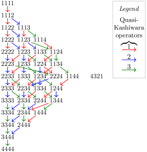
Figure 5. The connected components $\Gamma({\smash{\mathrm{hypo}}}_{4},1111)$ and $\Gamma({\smash{\mathrm{hypo}}}_{4},4321)$ of the quasi-crystal graph $\Gamma({\smash{\mathrm{hypo}}}_{4})$. These are also the connected components $\Gamma({\smash{\mathrm{plac}}}_{4},1111)$ and $\Gamma({\smash{\mathrm{plac}}}_{4},4321)$ of the crystal graph $\Gamma({\smash{\mathrm{plac}}}_{4})$: there is no vertex in these components where some $\tilde{e}_{i}$ or $\tilde{f}_{i}$ is defined but the corresponding $\ddot{e}_{i}$ or $\ddot{f}_{i}$ is not. These two components are not isomorphic to any other components of either $\Gamma({\smash{\mathrm{hypo}}}_{4})$ or $\Gamma({\smash{\mathrm{plac}}}_{4})$. The other components of $\Gamma({\smash{\mathrm{hypo}}}_{n})$ and $\Gamma({\smash{\mathrm{plac}}}_{n})$ whose vertices are length-$4$ words are shown in Figures 6 and 7.

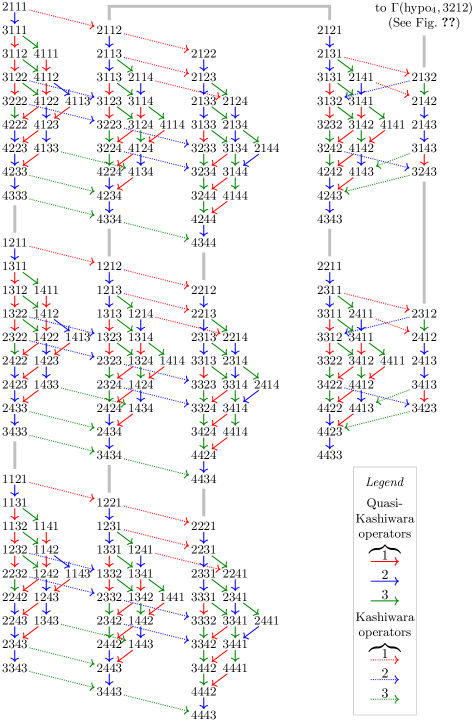
Figure 6. Thirteen components of $\Gamma({\smash{\mathrm{hypo}}}_{4})$, which together lie inside five components of $\Gamma({\smash{\mathrm{plac}}}_{n})$. Dotted lines show actions of operators $\tilde{e}_{i}$ and $\tilde{f}_{i}$ that are not also actions of operators $\ddot{e}_{i}$ and $\ddot{f}_{i}$. Each of these components of $\Gamma({\smash{\mathrm{hypo}}}_{4})$ is isomorphic to at least one other component; grey lines link isomorphic components. Other components are shown in Figures 5 and 7.

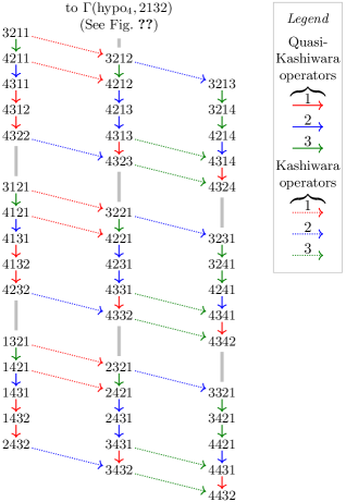
Figure 7. Nine components of $\Gamma({\smash{\mathrm{hypo}}}_{4})$, which together lie inside three of the connected components $\Gamma({\smash{\mathrm{plac}}}_{n})$. Dotted lines show actions of operators $\tilde{e}_{i}$ and $\tilde{f}_{i}$ that are not also actions of operators $\ddot{e}_{i}$ and $\ddot{f}_{i}$. Each of these components of $\Gamma({\smash{\mathrm{hypo}}}_{4})$ is isomorphic to at least one other component; grey lines link isomorphic components. The other components whose vertices are length-$4$ words are shown in Figures 5 and 6.

8.1. Sizes of classes and quasi-crystals

As previously noted, by fixing a Young tableau $P$ and varying $Q$ over all standard Young tableaux of the same shape as $P$, one obtains the plactic class corresponding to $P$. Notice that one obtains as a corollary that the size of this class depends on the shape of $P$, not on the entries of $P$. The so-called hook-length formula gives the number of standard Young tableaux of a given shape (see [FRT54] and [Ful97, § 4.3]) and thus of the size of a plactic class corresponding to an element of that shape.

This section uses the quasi-crystal graph to give an analogue of the hook-length formula for quasi-ribbon tableaux, in the sense of stating a formula for the size of hypoplactic classes corresponding to quasi-ribbon tableau of a given shape. Novelli [Nov00, Theorem 5.1] proves that for any compositions $\alpha=(\alpha_{1},\ldots,\alpha_{h})$ and $\gamma$,

(8.1) $$\sum_{\beta\preceq\alpha}\#(\beta,\gamma)=\binom{\alpha_{1}+\ldots+\alpha_{h}}{\alpha_{1},\ldots,\alpha_{h}},$$

where $\#(\beta,\gamma)$ is the size of the hypoplactic class corresponding to the quasi-ribbon tableau of shape $\beta$ and content $\gamma$. (Recall that $\beta\preceq\alpha$ denotes that $\beta$ is a coarser composition than $\alpha$; see Section 4.) Since the size of the hypoplactic class corresponding to a quasi-ribbon tableau of shape $(\alpha_{1})$ is always $1$, the formula (8.1) allows one to iteratively compute the size of an arbitrary hypoplactic class.

However, it is not immediately clear from (8.1) that the size of a hypoplactic class is only dependent on the shape of the quasi-ribbon tableau, not on its content:

Proposition 8.1.

Hypoplactic classes corresponding to quasi-ribbon tableaux of the same shape all have the same size.

Proof.

Let $u,v\in\mathcal{A}_{n}^{*}$ be such that $\mathrm{QR}\lparen u\rparen$ and $\mathrm{QR}\lparen v\rparen$ have the same shape. Then $\mathrm{C}\lparen\mathrm{QR}\lparen u\rparen\rparen$ and $\mathrm{C}\lparen\mathrm{QR}\lparen v\rparen\rparen$ lie in the same connected component by Proposition 6.4(1). Thus there is a sequence $\ddot{g}_{i_{1}},\ldots,\ddot{g}_{i_{r}}$ of operators $\ddot{e}_{i}$ and $\ddot{f}_{i}$ such that $\ddot{g}_{i_{1}}\cdots\ddot{g}_{i_{r}}(\mathrm{C}\lparen\mathrm{QR}\lparen u\rparen\rparen)=\mathrm{C}\lparen\mathrm{QR}\lparen v\rparen\rparen$. Each $\ddot{e}_{i}$ and $\ddot{f}_{i}$, when defined, is a bijection between $\equiv_{\smash{\mathrm{hypo}}}$-classes, and so $\big{[}\mathrm{C}\lparen\mathrm{QR}\lparen u\rparen\rparen\big{]}_{\equiv_{\smash{\mathrm{hypo}}}}$ and $\big{[}\mathrm{C}\lparen\mathrm{QR}\lparen v\rparen\rparen\big{]}_{\equiv_{\smash{\mathrm{hypo}}}}$ have the same size. Since $u\sim\mathrm{C}\lparen\mathrm{QR}\lparen u\rparen\rparen$ and $v\sim\mathrm{C}\lparen\mathrm{QR}\lparen v\rparen\rparen$, it follows that $[u]_{\equiv_{\smash{\mathrm{hypo}}}}$ and $[v]_{\equiv_{\smash{\mathrm{hypo}}}}$ have the same size. ∎

The formula for the size of hypoplactic classes is also straightforward when one uses the quasi-crystal graph:

Theorem 8.2.

The size of any hypoplactic class in $\mathcal{A}_{n}^{*}$ whose quasi-ribbon tableau has shape $\alpha$ is

(8.2) $$\begin{cases}{\displaystyle\sum_{\beta\preceq\alpha}(-1)^{\ell\lparen\alpha\rparen-\ell\lparen\beta\rparen}\binom{\lvert\beta\rvert}{\beta_{1},\cdots,\beta_{\ell\lparen\beta\rparen}}}&\text{if $\ell\lparen\alpha\rparen\leq n$,}\\ 0&\text{otherwise.}\end{cases}$$

Proof.

Note first that in a quasi-ribbon tableau, any symbol in $\mathcal{A}_{n}$ must lie in the first $n$ rows. Thus if $\ell\lparen\alpha\rparen>n$, then there is no quasi-ribbon tableau of shape $\alpha$ with entries in $\mathcal{A}_{n}$ and so the corresponding hypoplactic class if empty. So assume henceforth that $\ell\lparen\alpha\rparen\leq n$.

Let $T$ be a quasi-ribbon tableau of shape $\alpha$; the aim is to describe the cardinality of the set $U_{T}=\{\,u\in\mathcal{A}_{n}^{*}:\mathrm{QR}\lparen u\rparen=T\,\}$. Since the operators $\ddot{e}_{i}$ and $\ddot{f}_{i}$ are bijections between hypoplactic classes, assume without loss of generality that $\mathrm{C}\lparen T\rparen$ is highest-weight. By Corollary 6.5, $\mathrm{wt}\lparen\mathrm{C}\lparen T\rparen\rparen=\alpha$. Since all words in a hypoplactic class have the same weight, every word in $U_{T}$ has weight $\alpha$ (and thus contains exactly $\alpha_{i}$ symbols $i$, for each $i\in\mathcal{A}_{n}$). Furthermore, all words in $U_{T}$ are highest-weight and so have $i$-inversions for each $i\in\{1,\ldots,\ell\lparen\alpha\rparen\}$. Thus $U_{T}$ consists of exactly the words of weight $\alpha$, but that do not have the property of containing all symbols $i$ to the left of all symbols $i+1$ for some $i\in\{1,\ldots,\ell\lparen\alpha\rparen-1\}$.

For any weak composition $\gamma$ with $\ell\lparen\gamma\rparen\leq n$, the number of words in $\mathcal{A}_{n}^{*}$ with weight $\gamma$ is

$$\binom{\lvert\gamma\rvert}{\gamma_{1},\cdots,\gamma_{\ell\lparen\gamma\rparen}}.$$

Consider a word $u\in\mathcal{A}_{n}^{*}$ with $\mathrm{wt}\lparen u\rparen=\gamma$ that is $i$-inversion-free. Then in $u$, every symbol $i$ lies to the left of every symbol $i+1$. Replacing each symbol $j+1$ by $j$ for each $j\geq i$ yields a word $u^{\prime}$ with weight $\gamma^{\prime}=(\gamma_{1},\ldots,\gamma_{i-1},\gamma_{i}+\gamma_{i+1},\gamma_{i+2}\ldots,\gamma_{n})$; note that $\gamma^{\prime}\preceq\gamma$ and $\ell\lparen\gamma^{\prime}\rparen=\ell\lparen\gamma\rparen-1$. On the other hand, starting from $u^{\prime}$ and replacing each symbol $j$ by $j+1$ for $j\geq i+1$ and replacing the rightmost $\gamma_{i+1}$ symbols $i$ by $i+1$ yields $u$. Thus there is a one-to-one correspondence between words of weight $\gamma$ that are $i$-inversion-free and words of weight $\gamma^{\prime}$.

Iterating this argument shows that there is a one-to-one correspondence between words of weight $\gamma$ that are $i$-inversion-free for $i\in I\subseteq\{1,\ldots,n-1\}$ and words of weight $\gamma_{I}$ for a (uniquely determined) $\gamma_{I}\preceq\gamma$.

Hence, by the inclusion–exclusion principle, the number of such words that are $i$-inversion-free for all $i\in\{1,\ldots,n-1\}$ is given by (8.2). ∎

For example, let $\alpha=(2,1,1,2)$. By Theorem 8.2, the size of the hypoplactic class whose quasi-ribbon tableau has shape $\alpha$ is

$$\frac{6!}{2!1!1!2!} -\frac{6!}{3!1!2!}-\frac{6!}{2!2!2!}-\frac{6!}{2!1!3!}$$

$$+\frac{6!}{4!2!}+\frac{6!}{3!3!}+\frac{6!}{2!4!}$$

$$-\frac{6!}{6!}=19.$$

The quasi-ribbon word $143214$ corresponds to a quasi-ribbon tableau with shape $\alpha$, and the hypoplactic class containing $u$ is

$$\{ 143214,413214,431214,432114,$$

$$143241,413241,431241,432141,$$

$$143421,413421,431421,432411,$$

$$144321,414321,434121,434211,$$

$$\phantom{414321,}\,441321,443121,443211\},$$

which contains $19$ elements, as expected.

For the sake of completeness, this section closes with a formula for the number of quasi-ribbon tableaux of a given shape, which allows one to compute the size of a connected component of $\Gamma({\smash{\mathrm{hypo}}}_{n})$. Notice that the proof of this does not depend on applying the crystal structure.

Theorem 8.3.

The number of quasi-ribbon tableaux of shape $\alpha$ and symbols from $\mathcal{A}_{n}$ is

$$\begin{cases}\binom{n+\lvert\alpha\rvert-\ell\lparen\alpha\rparen}{n-\ell\lparen\alpha\rparen}&\text{if $\ell\lparen\alpha\rparen\leq n$}\\ 0&\text{if $\ell\lparen\alpha\rparen>n$}.\end{cases}$$

Proof.

Consider a ribbon diagram of shape $\alpha$, where the boundaries between the cells, including the left boundary of the first cell and the right boundary of the last cell, are indexed by the numbers $0,1,\ldots,\lvert\alpha\rvert$. Notice that $D(\alpha)$ be the set of indices of boundaries between vertically adjacent cells. For example, for shape $\alpha=(4,4,2,3)$, the indices are as follows:

In this case, $D(\alpha)=\{4,8,10\}$.

A filling of such a quasi-ribbon tableau by symbols from $\mathcal{A}_{n}$ is weakly increasing from upper left to lower right, and is specified exactly by listing $n-1$ boundaries between adjacent cells where the increase from $i$ to $i+1$ occurs in this filling. Note that such a list may contain repeated entries (and is thus formally a multiset), indicating that the difference between the entries in the cells incident on this boundary differ by more than $1$. For example, for $n=9$ the filling

corresponds to the multiset

$$\langle 0,1,1,4,6,7,8,10\rangle.$$

Note that this multiset has length $n-1=8$ and contains the entry $0$, indicating the presence of $2$ in the first cell, and a repeated entry $1$, indicating the jump from $2$ to $4$ at this boundary. However, some of the entries in this multiset are forced by the shape of the tableau: there must be increases at boundaries $4$, $8$, and $10$, which are between vertically adjacent cells.

There is thus a one-to-one correspondence between multisets with $n-1$ elements drawn from $\{0,\ldots,\lvert\alpha\rvert\}$ and that contain $D(\alpha)$ (which indicates the position of the ‘forced’ increases) and fillings of a tableau of shape $\alpha$. Since $|D(\alpha)|=\ell\lparen\alpha\rparen-1$, the number of such multisets is $0$ if $\ell\lparen\alpha\rparen>n$, and is otherwise the number of multisets with $(n-1)-(\ell\lparen\alpha\rparen-1)$ elements drawn from $\{0,\ldots,\lvert\alpha\rvert\}$, which is $\binom{(\lvert\alpha\rvert+1)+((n-1)-(\ell\lparen\alpha\rparen-1))-1}{(n-1)-(\ell\lparen\alpha\rparen-1)}$ by the standard formula for the number of multisets [Sta12, § 1.2], which simplifies to $\binom{n+\lvert\alpha\rvert-\ell\lparen\alpha\rparen}{n-\ell\lparen\alpha\rparen}$. ∎

8.2. Interaction of the crystal and quasi-crystal graphs

This section examines the interactions of the crystal graph $\Gamma({\smash{\mathrm{plac}}}_{n})$ and quasi-crystal graph $\Gamma({\smash{\mathrm{hypo}}}_{n})$. The first, and most fundamental, observation, is how connected components in $\Gamma({\smash{\mathrm{plac}}}_{n})$ are made up of connected components in $\Gamma({\smash{\mathrm{hypo}}}_{n})$:

Proposition 8.4.

The vertex set of every connected component of $\Gamma({\smash{\mathrm{plac}}}_{n})$ is a union of vertex sets of connected components of $\Gamma({\smash{\mathrm{hypo}}}_{n})$.

Proof.

By Proposition 5.2, any edge in $\Gamma({\smash{\mathrm{hypo}}}_{n})$ (whose edges indicate the action of the quasi-Kashiwara operators $\ddot{e}_{i}$ and $\ddot{f}_{i}$) is also an edge in $\Gamma({\smash{\mathrm{plac}}}_{n})$ (whose edges indicate the action of the Kashiwara operators $\tilde{e}_{i}$ and $\tilde{f}_{i}$). Hence every connected component in $\Gamma({\smash{\mathrm{hypo}}}_{n})$ lies entirely within a connected component of $\Gamma({\smash{\mathrm{plac}}}_{n})$; the result follows immediately. ∎

For example, as shown in Figure 6, the connected component $\Gamma({\smash{\mathrm{plac}}}_{4},2111)$ is made up of the three connected components $\Gamma({\smash{\mathrm{hypo}}}_{4},2111)$, $\Gamma({\smash{\mathrm{hypo}}}_{4},2112)$, and $\Gamma({\smash{\mathrm{hypo}}}_{4},2122)$.

Proposition 8.5.

Let $\Theta:\Gamma({\smash{\mathrm{plac}}}_{n},u)\to\Gamma({\smash{\mathrm{plac}}}_{n},\Theta(u))$ be a crystal isomorphism. Then $\Theta$ restricts to a quasi-crystal isomorphism from $\Gamma({\smash{\mathrm{hypo}}}_{n},w)$ to $\Gamma({\smash{\mathrm{hypo}}}_{n},\Theta(w))$, for all $w\in\Gamma({\smash{\mathrm{plac}}}_{n},u)$.

Proof.

Let $\Theta:\Gamma({\smash{\mathrm{plac}}}_{n},u)\to\Gamma({\smash{\mathrm{plac}}}_{n},\Theta(u))$ be a crystal isomorphism and let $w\in\Gamma({\smash{\mathrm{plac}}}_{n},u)$. Suppose the Kashiwara operator $\tilde{f}_{i}$ is defined on $w$ but the quasi-Kashiwara operator $\ddot{f}_{i}$ is not defined on $w$. Since $\tilde{f}_{i}$ is defined, $w$ must contain at least one symbol $i$. Thus, since $\ddot{f}_{i}$ is undefined, $w$ must have an $i$-inversion. Since $\Theta$ is a crystal isomorphism, $w\equiv_{\smash{\mathrm{plac}}}\Theta(w)$. The defining relations in $\mathcal{R}_{\smash{\mathrm{plac}}}$ preserve the property of having $i$-inversions (for if a defining relation in $\mathcal{R}_{\smash{\mathrm{plac}}}$ commutes a symbol $i$ and $i+1$, then $a=i$ and $c=i+1$ in this defining relation, and so $b\in\{i,i+1\}$, and so the applied relation is either $(i(i+1)i,(i+1)ii)$ or $((i+1)i(i+1),(i+1)(i+1)i)$, and both sides of these relations have $i$-inversions). Hence $\Theta(w)$ has an $i$-inversion. Hence $\ddot{f}_{i}$ is not defined on $w$.

A symmetric argument shows that if $\tilde{f}_{i}$ is defined on $\Theta(w)$ but $\ddot{f}_{i}$ is not, then $\ddot{f}_{i}$ is not defined on $w$. Hence the isomorphism $\Theta$ maps edges corresponding to actions of quasi-Kashiwara operators in $\Gamma({\smash{\mathrm{plac}}}_{n},u)$ to edges corresponding to actions of quasi-Kashiwara operators in $\Gamma({\smash{\mathrm{plac}}}_{n},\Theta(u))$, and vice versa, and so restricts to a quasi-crystal isomorphism from $\Gamma({\smash{\mathrm{hypo}}}_{n},w)$ to $\Gamma({\smash{\mathrm{hypo}}}_{n},\Theta(w))$ for all $w\in\Gamma({\smash{\mathrm{plac}}}_{n},u)$. ∎

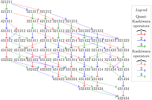
Figure 8. The connected component $\Gamma({\smash{\mathrm{plac}}}_{4},321211)$, drawn so that the connected components of $\Gamma({\smash{\mathrm{hypo}}}_{4})$ are arranged vertically. Notice that it contains the isomorphic connected components $\Gamma({\smash{\mathrm{hypo}}}_{4},321213)$ and $\Gamma({\smash{\mathrm{hypo}}}_{4},321312)$, and also the isomorphic one-vertex connected components $\Gamma({\smash{\mathrm{hypo}}}_{4},421323)$ and $\Gamma({\smash{\mathrm{hypo}}}_{4},321423)$.

Notice that it is possible for a single connected component of $\Gamma({\smash{\mathrm{plac}}}_{n})$ to contain distinct isomorphic connected components of $\Gamma({\smash{\mathrm{hypo}}}_{n})$. For example, as shown in Figure 8, the connected component $\Gamma({\smash{\mathrm{plac}}}_{4},321211)$ contains the isomorphic connected components $\Gamma({\smash{\mathrm{hypo}}}_{4},321213)$ and $\Gamma({\smash{\mathrm{hypo}}}_{4},321312)$.

Note also that $\Gamma({\smash{\mathrm{plac}}}_{4},321211)$, contains the isomorphic one-vertex connected components $\Gamma({\smash{\mathrm{hypo}}}_{4},421323)$ and $\Gamma({\smash{\mathrm{hypo}}}_{4},321423)$. (There are other one-vertex components of $\Gamma({\smash{\mathrm{hypo}}}_{4})$ inside $\Gamma({\smash{\mathrm{plac}}}_{4},321211)$, but these have different weights and so there are no quasi-crystal isomorphisms between them.) The quasi-ribbon tableau $\mathrm{QR}\lparen 421323\rparen$ has shape $(1,2,2,1)$; thus, by Theorem 8.2, the hypoplactic class containing $421323$ has size

$$\frac{6!}{1!2!2!1!} -\frac{6!}{3!2!1!}-\frac{6!}{1!4!1!}-\frac{6!}{1!2!3!}$$

$$+\frac{6!}{5!1!}+\frac{6!}{3!3!}+\frac{6!}{1!5!}$$

$$-\frac{6!}{6!}=61.$$

Since there are an odd number of components that are isomorphic to $\Gamma({\smash{\mathrm{hypo}}}_{4},421323)$, it follows that there must be at least one component of $\Gamma({\smash{\mathrm{plac}}}_{4})$ that contains an odd number of these components. Thus different components of $\Gamma({\smash{\mathrm{plac}}}_{4})$ may contain different numbers of isomorphic components of $\Gamma({\smash{\mathrm{hypo}}}_{4})$.

Corollary 8.6.

Let $u,v\in\mathcal{A}_{n}^{*}$ be such that $u\equiv_{\smash{\mathrm{plac}}}v$ but $u\neq v$, so that there is a non-trivial crystal isormorphism $\Theta:\Gamma({\smash{\mathrm{plac}}}_{n},u)\to\Gamma({\smash{\mathrm{plac}}}_{n},v)$ with $\Theta(u)=v$. Let $s\in\Gamma({\smash{\mathrm{plac}}}_{n},u)$ and $t\in\Gamma({\smash{\mathrm{plac}}}_{n},v)$ be quasi-ribbon words. Then $\Theta$ does not map $\Gamma({\smash{\mathrm{hypo}}}_{n},s)$ to $\Gamma({\smash{\mathrm{hypo}}}_{n},t)$. More succinctly, quasi-ribbon word components of $\Gamma({\smash{\mathrm{hypo}}}_{n})$ cannot lie in the same places in distinct isomorphic components of $\Gamma({\smash{\mathrm{plac}}}_{n})$.

Proof.

Without loss of generality, assume $s$ and $t$ are highest-weight in $\Gamma({\smash{\mathrm{hypo}}}_{n},s)$ and $\Gamma({\smash{\mathrm{hypo}}}_{n},t)$ respectively. Suppose, with the aim of obtaining a contradiction, that $\Theta$ maps $\Gamma({\smash{\mathrm{hypo}}}_{n},s)$ to $\Gamma({\smash{\mathrm{hypo}}}_{n},t)$. Then $\Theta(s)=t$, and so $s\equiv_{\smash{\mathrm{hypo}}}t$. Since $s$ and $t$ are quasi-ribbon words, $s=t$ by Proposition 6.4 and so $\Theta$ is trivial, which is a contradiction. ∎

Corollary 6.2 showed that the quasi-Kashiwara operators preserve shapes of quasi-ribbon tableau. In fact, quasi-Kashiwara operators and, more generally, Kashiwara operators, preseve shapes of quasi-ribbon tabloids (see Section 4 for the definitions of quasi-ribbon tabloids):

Proposition 8.7.

Let $i\in\{1,\ldots,n-1\}$. Let $u\in\mathcal{A}_{n}^{*}$.

1. If the Kashiwara operator $\tilde{e}_{i}$ is defined on $u$, then $\mathrm{QRoid}\lparen\tilde{e}_{i}(u)\rparen$ and $\mathrm{QRoid}\lparen u\rparen$ have the same shape.

2. If the Kashiwara operator $\tilde{f}_{i}$ is defined on $u$, then $\mathrm{QRoid}\lparen\tilde{f}_{i}(u)\rparen$ and $\mathrm{QRoid}\lparen u\rparen$ have the same shape.

Proof.

Let $u\in\mathcal{A}_{n}^{*}$ and let $u=u^{(1)}\cdots u^{(m)}$ be the factorization of $u$ into maximal decreasing factors (which are entries of the columns of $\mathrm{QRoid}\lparen u\rparen$).

Suppose that the Kashiwara operator $\tilde{e}_{i}$ is defined on $u$, and that the application of $\tilde{e}_{i}$ to $u$ replaces the (necessarily unique) symbol $i+1$ in $u^{(k)}$ by a symbol $i$; let $\hat{u}^{(k)}$ be the result of this replacement. Then $u^{(k)}$ cannot contain a symbol $i$, for if it did, then during the computation of the action of $\tilde{e}_{i}$ as described in Subsection 3.3, the symbols $i+1$ and $i$ in $u^{(k)}$ (which would be adjacent since $u^{(k)}$ is strictly decreasing) would have been replaced by $-$ and $+$ and so would have been deleted, and so $\tilde{e}_{i}$ would not act on this symbol $i+1$. Hence $\hat{u}^{(k)}$ is also a decreasing word.

Furthermore, the first symbol of $u^{(k+1)}$ is greater than or equal to the last symbol of $u^{(k)}$, and so is certainly greater than or equal to the last symbol of $\hat{u}^{(k)}$ since $\tilde{e}_{i}$ can only decrease a symbol.

Similarly, the first symbol of $u^{(k)}$ is greater than or equal to the last symbol of $u^{(k-1)}$. If $u^{(k)}$ does not start with the symbol $i+1$, the first symbol of $\hat{u}^{(k)}$ is greater than or equal to the last symbol of $u^{(k-1)}$. So assume $u^{(k)}$ starts with the symbol $i+1$; since the factorization is into maximal decreasing factors, $u^{(k-1)}$ ends with a symbol that is less than or equal to $i+1$. If $u^{(k-1)}$ ends with a symbol that is strictly less than $i+1$, then the first symbol of $\hat{u}^{(k)}$ is greater than or equal to the last symbol of $u^{(k-1)}$. So assume $u^{(k-1)}$ ends with the symbol $i+1$. Then during the computation of the action of $\tilde{e}_{i}$ as described in Subsection 3.3, the adjacent symbols $i+1$ at the end of $u^{(k-1)}$ and at the start of $u^{(k)}$ are both replaced by symbols $-$, and neither of these symbols are removed by deletion of factors ${-}{+}$, since $\tilde{e}_{i}$ acts on the symbol $i+1$ at the start of $u^{(k)}$. But this contradicts the fact that $\tilde{e}_{i}$ acts on the symbol replaced by the leftmost ${-}$. Thus this case cannot arise, and so one of the previous possibilities must have held true.

Combining the last three paragraphs shows that the factorization of $\tilde{e}_{i}(u)$ into maximal decreasing factors is $\tilde{e}_{i}(u)=u^{(1)}\cdots u^{(k-1)}\hat{u}^{(k)}u^{(k+1)}\cdots u^{(m)}$. This proves part (1). Similar reasoning for $\tilde{f}_{i}$ proves part (2). ∎

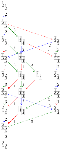
Figure 9. The component $\Gamma({\smash{\mathrm{plac}}}_{4},2121)$, with words drawn as quasi-ribbon tabloids of the same shape. Only the component $\Gamma({\smash{\mathrm{hypo}}}_{4},2132)$ consists of quasi-ribbon words, which thus appear here as quasi-ribbon tableaux.

Proposition 8.8.

A connected component of $\Gamma({\smash{\mathrm{plac}}}_{n})$ contains at most one quasi-ribbon word component of $\Gamma({\smash{\mathrm{hypo}}}_{n})$.

Proof.

Suppose the connected component $\Gamma({\smash{\mathrm{plac}}}_{n},u)$ contains connected components $\Gamma({\smash{\mathrm{hypo}}}_{n},w)$ and $\Gamma({\smash{\mathrm{hypo}}}_{n},w^{\prime})$ that both consist of quasi-ribbon words. Without loss of generality, assume that $w$ is highest- weight in $\Gamma({\smash{\mathrm{hypo}}}_{n},w)$ and $w^{\prime}$ has highest-weight in $\Gamma({\smash{\mathrm{hypo}}}_{n},w^{\prime})$. Since $w$ and $w^{\prime}$ are in the connected component $\Gamma({\smash{\mathrm{plac}}}_{n},u)$, the quasi-ribbon tableaux $\mathrm{QR}\lparen w\rparen$ and $\mathrm{QR}\lparen w^{\prime}\rparen$ have the same shape by Proposition 8.7. Hence by Corollary 6.5, $\mathrm{wt}\lparen w\rparen=\mathrm{wt}\lparen w^{\prime}\rparen$ and so $w=w^{\prime}$ by Corollary 6.6. Thus $\Gamma({\smash{\mathrm{hypo}}}_{n},w)=\Gamma({\smash{\mathrm{hypo}}}_{n},w^{\prime})$. ∎

It is possible that a connected component of $\Gamma({\smash{\mathrm{plac}}}_{n})$ contains no quasi-ribbon word components of $\Gamma({\smash{\mathrm{hypo}}}_{n})$. For example, as can be seen in Figure 6, $\Gamma({\smash{\mathrm{plac}}}_{4},2211)$ contains the connected components $\Gamma({\smash{\mathrm{hypo}}}_{4},2211)$ and $\Gamma({\smash{\mathrm{hypo}}}_{4},2312)$, and neither $2211$ nor $2312$ is a quasi-ribbon word. Thus the next aim is to characterize those connected components of $\Gamma({\smash{\mathrm{plac}}}_{n})$ that contain a (necessarily unique) quasi-ribbon word component of $\Gamma({\smash{\mathrm{hypo}}}_{n})$. In order to do this, it is useful to discuss a shortcut that allows one to calculate quickly the Young tableau $\mathrm{P}\lparen w\rparen$ obtained when $w$ is a quasi-ribbon word.

The slide up–slide left algorithm takes a filled quasi-ribbon diagram $D$ and produces a filled Young diagram as follows: Start from the quasi-ribbon diagram $D$. Slide all the columns upwards until the topmost entry of each is on row $1$. Now slide all the symbols leftwards along their rows until the leftmost entry in each row is in the first column and there are no gaps in each row.

As will be shown in Proposition 8.9(1), applying the slide up–slide left algorithm to a quasi-ribbon tableau $\mathrm{QR}\lparen u\rparen$ gives the Young tableau $\mathrm{P}\lparen u\rparen$, as in the following example:

Similarly, as will be shown in Proposition 8.9(2), applying the slide up–slide left algorithm to a quasi-ribbon tableau of the same shape $\alpha$ as $\mathrm{QR}\lparen u\rparen$, filled with entries $1,\ldots,\ell\lparen\alpha\rparen$, gives the standard Young tableau $\mathrm{Q}\lparen u\rparen$, as in the following example:

Proposition 8.9.

Let $T$ be a quasi-ribbon tableau of shape $\alpha$.

1. Applying the slide up–slide left algorithm to $T$ yields the Young tableau $\mathrm{P}\lparen\mathrm{C}\lparen T\rparen\rparen$.

2. Applying the slide up–slide left algorithm to the (unique) quasi-ribbon tableau of shape $\alpha$ filled with entries $1,\ldots,\lvert\alpha\rvert$ yields the standard Young tableau $\mathrm{Q}\lparen\mathrm{C}\lparen T\rparen\rparen$.

Proof.

Let $U$ be the unique quasi-ribbon tableau of shape $\alpha$ filled with entries $1,\ldots,\lvert\alpha\rvert$. The proof is by induction on the number of columns $m$ in a ribbon diagram of shape $\alpha$.

Suppose $m=1$. Then applying the slide up–slide left algorithm to $T$ and $U$ yields $T$ and $U$, respectively (viewed as filled Young diagrams). Since $T$ satisifies the condition for being a Young tableau, $\mathrm{P}\lparen\mathrm{C}\lparen T\rparen\rparen=T$. Furthermore, $U$ is also the unique standard Young tableau with a single column of the same shape as $T$, and so must be $\mathrm{Q}\lparen\mathrm{C}\lparen T\rparen\rparen$.

Now suppose $m>1$ and that the result holds for all quasi-ribbon tableau $T^{\prime}$ with fewer than $m$ columns. In particular, it holds for the quasi-ribbon tableau $T^{\prime}$ formed by the first $m-1$ columns of $T$. In particular, by applying the slide up–slide left algorithm to $T^{\prime}$, one obtains $\mathrm{P}\lparen\mathrm{C}\lparen T^{\prime}\rparen\rparen$. If the $m$-th column of $T$ contains entries $a_{1},\ldots,a_{k}$ (listed from bottom to top, so that $a_{1}>\ldots>a_{k}$), then applying the slide up–slide left algorithm to $T$ yields the filled Young diagram obtained by applying it to $T^{\prime}$ (which yields $\mathrm{P}\lparen\mathrm{C}\lparen T^{\prime}\rparen\rparen$) and then adding the symbol $a_{h}$ at the rightmost end of the $h$-th row. Since each symbol $a_{1},\ldots,a_{k}$ is greater or equal to than every symbol in $T^{\prime}$ and thus in $\mathrm{P}\lparen\mathrm{C}\lparen T^{\prime}\rparen\rparen$, using Algorithm 4.2 to insert the symbols $a_{1},\ldots,a_{k}$ into $\mathrm{P}\lparen\mathrm{C}\lparen T^{\prime}\rparen\rparen$ does not involve bumping any symbols in $\mathrm{P}\lparen\mathrm{C}\lparen T^{\prime}\rparen\rparen$. That is, the symbols $a_{1},\ldots,a_{k}$ (which form a strictly decreasing sequence) bump each other up the rightmost edge of $\mathrm{P}\lparen\mathrm{C}\lparen T^{\prime}\rparen\rparen$, as in the following example

$$\leavevmode\hbox to99.98pt{\vbox to57.31pt{\text{[drawing]}}}\leftarrow a_{4}=\leavevmode\hbox to99.98pt{\vbox to57.31pt{\text{[drawing]}}} {a_{3}} {a_{2}} {a_{1}} \mathrm{P}\lparen\mathrm{C}\lparen T^{\prime}\rparen\rparen {a_{4}} {a_{3}} {a_{2}} {a_{1}} \mathrm{P}\lparen\mathrm{C}\lparen T^{\prime}\rparen\rparen {a_{3}} {a_{2}} {a_{1}} \mathrm{P}\lparen\mathrm{C}\lparen T^{\prime}\rparen\rparen {a_{4}} {a_{3}} {a_{2}} {a_{1}} \mathrm{P}\lparen\mathrm{C}\lparen T^{\prime}\rparen\rparen$$

Furthermore, applying the slide up–slide left algorithm to the unique quasi-ribbon tableau of the same shape as $T^{\prime}$ filled with entries $1,\ldots,(\lvert\alpha\rvert-k)$ yields the standard Young tableau $\mathrm{Q}\lparen\mathrm{C}\lparen T^{\prime}\rparen\rparen$. Thus applying the slide up–slide left algorithm to the unique quasi-ribbon tableau of shape $\alpha$ filled with entries $1,\ldots,\lvert\alpha\rvert$ yields the filled Young diagram obtained by applying it to $\mathrm{Q}\lparen\mathrm{C}\lparen T^{\prime}\rparen\rparen$ and adding $\lvert\alpha\rvert-k+h$ to the end of the $h$-th row for $h=1,\ldots,k$. By the above analysis of the behaviour of Algorithm 4.2, this is the standard Young tableau $\mathrm{Q}\lparen\mathrm{C}\lparen T\rparen\rparen$. ∎

Proposition 8.10.

Let $Q$ be a standard Young tableau. There is at most one quasi-ribbon tableau $T$ such that $Q$ can be obtained by applying the slide up–slide left algorithm to $T$.

Proof.

Suppose that $T$ and $T^{\prime}$ are quasi-ribbon tableaux such that applying the slide up–slide left algorithm to $T$ and $T^{\prime}$ yields $Q$. Then by Proposition 8.9(1–2), $\mathrm{P}\lparen\mathrm{C}\lparen T\rparen\rparen=\mathrm{Q}\lparen\mathrm{C}\lparen T\rparen\rparen=Q=\mathrm{P}\lparen\mathrm{C}\lparen T^{\prime}\rparen\rparen=\mathrm{Q}\lparen\mathrm{C}\lparen T^{\prime}\rparen\rparen$. Thus by the Robinson–Schensted–Knuth correspondence, $\mathrm{C}\lparen T\rparen=\mathrm{C}\lparen T^{\prime}\rparen$ and so $T=T^{\prime}$. ∎

Proposition 8.11.

A connected component $\Gamma({\smash{\mathrm{plac}}}_{n},w)$ contains a quasi-ribbon word component if and only if $\mathrm{Q}\lparen w\rparen$ can be obtained by applying the slide up–slide left algorithm to some quasi-ribbon tableau $T$ of shape $\alpha$ and entries $1,\ldots,\lvert\alpha\rvert$ and such that $\ell\lparen\alpha\rparen\leq n$.

Proof.

Suppose $\Gamma({\smash{\mathrm{plac}}}_{n},w)$ contains a quasi-ribbon word component. Let $u\in\Gamma({\smash{\mathrm{plac}}}_{n},w)$ be a quasi-ribbon word. Let $\alpha$ be the shape of $\mathrm{QR}\lparen u\rparen$. Note that $\mathrm{QR}\lparen u\rparen$ has at most $n$ rows, so $\ell\lparen\alpha\rparen\leq n$. By Proposition 8.9(2), applying the slide up–slide left algorithm to the unique quasi-ribbon tableau of shape $\alpha$ filled with entries $1,\ldots,\lvert\alpha\rvert$ yields the standard Young tableau $\mathrm{Q}\lparen u\rparen$. Since $u$ and $w$ are in the same connected component of $\Gamma({\smash{\mathrm{plac}}}_{n})$, the standard Young tableaux $\mathrm{Q}\lparen w\rparen$ and $\mathrm{Q}\lparen u\rparen$ are equal.

On the other hand, suppose that $\mathrm{Q}\lparen w\rparen$ can be obtained by applying the slide up–slide left algorithm to some quasi-ribbon tableau $T$ of shape $\alpha$ and entries $1,\ldots,\lvert\alpha\rvert$ and such that $\ell\lparen\alpha\rparen\leq n$. Let $U$ be the quasi-ribbon tableau of shape $\alpha$ and entries in $\mathcal{A}_{n}$ such that $\mathrm{C}\lparen U\rparen$ is highest-weight in its component of $\Gamma({\smash{\mathrm{hypo}}}_{n})$; note that $U$ exists since $\ell\lparen\alpha\rparen\leq n$. Then by Proposition 8.9(2), $\mathrm{Q}\lparen\mathrm{C}\lparen U\rparen\rparen=\mathrm{Q}\lparen w\rparen$ since $U$ has shape $\alpha$. Hence $\mathrm{C}\lparen U\rparen\in\Gamma({\smash{\mathrm{plac}}}_{n},w)$. ∎

Define a permutation $\sigma$ of $\{1,\ldots,n\}$ to be interval-reversing if there is some composition $\alpha=(\alpha_{1},\ldots,\alpha_{k})$ with $\lvert\alpha\rvert=n$ such that for all $h=0,\ldots,k$, the permutation $\sigma$ preserves the interval $\{\alpha_{1}+\ldots+\alpha_{h}+1,\ldots,\alpha_{1}+\ldots+\alpha_{h+1}\}$ and reverses the order of its elements. (For $h=0$, this interval is $\{1,\ldots,\alpha_{1}\}$.) Thus, for example,

$$\begin{pmatrix}1&2&3&4&5&6&7&8\\ 1&5&4&3&2&8&7&6\\ \end{pmatrix}$$

is an interval-reversing permutation of $\{1,\ldots,8\}$, where the appropriate composition $\alpha$ is $(1,4,3)$. It is clear that there is only one choice for $\alpha$.

It is well-known that if $w$ is a standard word (and thus a permutation), then the Robinson–Schensted–Knuth correspondence associates $w$ with $(\mathrm{P}\lparen w\rparen,\mathrm{Q}\lparen w\rparen)$ and $w^{-1}$ with $(\mathrm{Q}\lparen w\rparen,\mathrm{P}\lparen w\rparen)$. That is, $\mathrm{Q}\lparen w\rparen=\mathrm{P}\lparen w^{-1}\rparen$ and $\mathrm{P}\lparen w\rparen=\mathrm{Q}\lparen w^{-1}\rparen$. Thus involutions are associated to pairs $(Q,Q)$, where $Q$ is a standard Young tableau.

Proposition 8.12.

A connected component $\Gamma({\smash{\mathrm{plac}}}_{n},w)$ contains a quasi-ribbon word component if and only if the Robinson–Schensted–Knuth correspondence associates $(\mathrm{Q}\lparen w\rparen,\mathrm{Q}\lparen w\rparen)$ with an interval-reversing involution.

Proof.

Suppose $\Gamma({\smash{\mathrm{plac}}}_{n},w)$ contains a quasi-ribbon word. By Proposition 8.11, $\mathrm{Q}\lparen w\rparen$ can be obtained by applying the slide up–slide left algorithm to some quasi-ribbon tableau $T$ of shape $\beta$ and entries $1,\ldots,\lvert\beta\rvert$ and such that $\ell\lparen\beta\rparen\leq n$. By Proposition 8.9(1–2), $\mathrm{P}\lparen\mathrm{C}\lparen T\rparen\rparen=\mathrm{Q}\lparen\mathrm{C}\lparen T\rparen\rparen=\mathrm{Q}\lparen w\rparen$. So the Robinson–Schensted–Knuth correspondence associates $(\mathrm{Q}\lparen w\rparen,\mathrm{Q}\lparen w\rparen)$ wih $\mathrm{C}\lparen T\rparen$. Let $\alpha=(\alpha_{1},\ldots,\alpha_{k})$ be such that $\alpha_{i}$ is the length of the $i$-th column of $T$. Then by the definition of $T$ and its column reading, $\mathrm{C}\lparen T\rparen$ is an interval-reversing permutation where the appropriate composition is $\alpha$.

On the other hand, suppose the Robinson–Schensted–Knuth correspondence associates $(\mathrm{Q}\lparen w\rparen,\mathrm{Q}\lparen w\rparen)$ with an interval-reversing involution $u$, where the appropriate composition is $\alpha=(\alpha_{1},\ldots,\alpha_{k})$. Note that $\mathrm{Q}\lparen w\rparen=\mathrm{P}\lparen u\rparen$ and $\mathrm{Q}\lparen w\rparen=\mathrm{Q}\lparen u\rparen$. Let $T$ be the quasi-ribbon tabloid $\mathrm{QRoid}\lparen u\rparen$. Then $\alpha_{i}$ is the length of the $i$-th column of $T$, which is filled with the image of the interval $\{\alpha_{1}+\ldots+\alpha_{i}+1,\ldots,\alpha_{1}+\ldots+\alpha_{i+1}\}$ since $u$ is an interval-reversing permutation. Since the elements in each interval are less than the elements in the next, the rows of $T$ are increasing from left to right and so $T$ is a quasi-ribbon tableau that is filled with the symbols $1,\ldots,|u|$. Note that $u=\mathrm{C}\lparen T\rparen$, and so $\mathrm{Q}\lparen w\rparen=\mathrm{Q}\lparen u\rparen=\mathrm{Q}\lparen\mathrm{C}\lparen T\rparen\rparen$. So by Proposition 8.9, $\mathrm{Q}\lparen w\rparen$ can be obtained from $T$ by applying the slide up–slide left algorithm. Hence $\Gamma({\smash{\mathrm{plac}}}_{n},w)$ contains a quasi-ribbon word by Proposition 8.11. ∎

Corollary 8.13.

Let $w\in\mathcal{A}_{n}^{*}$ and let $\lambda=(\lambda_{1},\ldots,\lambda_{\ell\lparen\lambda\rparen})$ be the shape of $\mathrm{P}\lparen w\rparen$. The number of connected components of $\Gamma({\smash{\mathrm{plac}}}_{n})$ that are isomorphic to $\Gamma({\smash{\mathrm{plac}}}_{n},w)$ and contain quasi-ribbon word components of $\Gamma({\smash{\mathrm{hypo}}}_{n})$ is

$$\begin{cases}{\displaystyle\binom{\lambda_{1}}{\lambda_{1}-\lambda_{2},\;\;\ldots,\;\;\lambda_{\ell\lparen\lambda\rparen-1}-\lambda_{\ell\lparen\lambda\rparen},\;\;\lambda_{\ell\lparen\lambda\rparen}}}&\text{if $\lvert\lambda\rvert-\lambda_{1}+1\leq n$,}\\ 0&\text{otherwise.}\end{cases}$$

Proof.

By Proposition 8.11, the number of such components is equal to the number of standard Young tableaux of shape $\lambda$ that can be obtained by applying the slide up–slide left algorithm to some quasi-ribbon tableau of some shape $\alpha$ and entries $1,\ldots,\lvert\alpha\rvert$ and such that $\ell\lparen\alpha\rparen\leq n$. By the definition of a quasi-ribbon diagram, the number of rows $\ell\lparen\alpha\rparen$ of such a diagram is equal to the total number of boxes minus the number of columns plus $1$ (since adjacent pairs of columns overlap in exactly one row). Since the slide up–slide left algorithm preserves the number of columns and the total number of boxes, this number of rows is $\lvert\lambda\rvert-\lambda_{1}+1$. Hence if $\lvert\lambda\rvert-\lambda_{1}+1>n$, there is no standard Young tableau that can be obtained in such a way. So suppose henceforth that $\lvert\lambda\rvert-\lambda_{1}+1\leq n$.

For any composition $\alpha$, there is exactly one quasi-ribbon tableau of shape $\alpha$ filled with symbols $1,\ldots,\lvert\alpha\rvert$, and each of them yields (under the slide up–slide left algorithm) a different standard Young tableau by Proposition 8.11. Furthermore, there is a one-to-one correspondence between compositions $\alpha$ and shapes of tabloids: one simply takes a ribbon diagram of shape $\alpha$ and applies the ‘slide up’ part of the slide up–slide left algorithm. Thus, to obtain the number of such quasi-ribbon tableaux that give the correct shape on applying the slide up–slide left algorithm, it suffices to count the number of tabloid shapes that have $\lambda_{j}$ cells on the $j$-th row, for each $j=1,\ldots,\ell\lparen\lambda\rparen$. This is equal to the number of tabloid shapes that have $\lambda_{1}$ cells on the first row and $\lambda_{j}-\lambda_{j+1}$ columns ending on the $j$-th row, which in turn is equal to the number of words of length $\lambda_{1}$ containing $\lambda_{j}-\lambda_{j+1}$ symbols $j$ for each $j<\ell\lparen\lambda\rparen$ and $\lambda_{\ell\lparen\lambda\rparen}$ symbols $\ell\lparen\lambda\rparen$. ∎

Note that the number of components specified by Corollary 8.13 is dependent only on the shape of $\mathrm{P}\lparen w\rparen$, not on $\mathrm{wt}\lparen w\rparen$ or $w$ itself. This is what one would expect in working with a class of isomorphic components in $\Gamma({\smash{\mathrm{plac}}}_{n})$.

Corollary 8.14.

Let $w\in\mathcal{A}_{n}^{*}$, and let $\lambda=(\lambda_{1},\ldots,\lambda_{m})$ be the shape of $\mathrm{P}\lparen w\rparen$. Suppose $\lvert\lambda\rvert-\lambda_{1}+1\leq n$. Then $\Gamma({\smash{\mathrm{plac}}}_{n},w)$ contains at least

$$\binom{\lambda_{1}}{\lambda_{1}-\lambda_{2},\;\;\ldots,\;\;\lambda_{\ell\lparen\lambda\rparen-1}-\lambda_{\ell\lparen\lambda\rparen},\;\;\lambda_{\ell\lparen\lambda\rparen}}$$

connected components of $\Gamma({\smash{\mathrm{hypo}}}_{n})$.

Proof.

Corollary 8.13 gives the number of components isomorphic to $\Gamma({\smash{\mathrm{plac}}}_{n},w)$ that contain quasi-ribbon word components. Each one of these quasi-ribbon word components is isomorphic to a connected component of $\Gamma({\smash{\mathrm{hypo}}}_{n})$ inside $\Gamma({\smash{\mathrm{plac}}}_{n},w)$ by Proposition 8.5, and to distinct such connected components of $\Gamma({\smash{\mathrm{hypo}}}_{n})$ by Corollary 8.6. Hence the number of connected components of $\Gamma({\smash{\mathrm{hypo}}}_{n})$ inside $\Gamma({\smash{\mathrm{plac}}}_{n},w)$ must be at least the number given in Corollary 8.13 in the case where $\lvert\lambda\rvert-\lambda_{1}+1\leq n$. ∎

8.3. The Schützenberger involution

The Schützenberger involution is the map ${}^{\sharp}:\mathcal{A}_{n}^{*}\to\mathcal{A}_{n}^{*}$ that sends $a\in\mathcal{A}_{n}$ to $n-a+1$ and is extended to $\mathcal{A}_{n}^{*}$ by ${(a_{1}\cdots a_{k})}^{\sharp}\mapsto{a_{k}}^{\sharp}\cdots{a_{1}}^{\sharp}$. That is, given a word, one obtains its image under ^♯ by reversing the word and replacing each symbol $a$ by $n-a+1$. It is well-known that the Schützenberger involution reverses the order of weights, in the sense that if $u$ has higher weight than $v$, then ${v}^{\sharp}$ has higher weight than ${u}^{\sharp}$.

Proposition 8.15.

In $\Gamma({\smash{\mathrm{hypo}}}_{n})$, the Schützenberger involution maps connected components to connected components. If there is an edge from $u$ to $v$ labelled by $i$, then there is an edge from ${v}^{\sharp}$ to ${u}^{\sharp}$ labelled by $n-i$.

Proof.

Clearly the second statement implies the first. So suppose that $\ddot{f}_{i}(u)=v$. Then $u$ contains at least one symbol $i$ and, every symbol $i$ is to the left of every symbol $i+1$, and $v$ is obtained from $u$ by replacing the rightmost symbol $i$ by $i+1$. By the definition of ^♯, in the word ${u}^{\sharp}$, every symbol $n-i+1$ is to the right of every symbol $n-i$. Hence $\ddot{e}_{n-i}({u}^{\sharp})$ is defined, is equal to the word obtained from ${u}^{\sharp}$ by replacing the leftmost symbol $n-i+1$ by $n-i$, which is ${v}^{\sharp}$. Hence there is an edge from ${v}^{\sharp}$ to ${u}^{\sharp}$ labelled by $n-i$. ∎

8.4. Characterizing quasi-crystal graphs?

Stembridge [Ste03] gives a set of axioms that characterize connected components of crystal graphs. These axioms specify ‘local’ conditions that the graph must satisfy. It is natural to ask whether there is an analogous characterization for quasi-crystal graphs:

Question 8.16.

Is there a local characterization of quasi-crystal graphs?

However, the Stembridge axioms are connected with the underlying representation theory, in the sense that they refer to whether the arrow labels correspond to orthogonal roots of the algebra. Since the quasi-crystal graphs are defined on a purely combinatorial level, any characterization of them must also be on a purely combinatorial level.

9. Applications

9.1. Counting factorizations

One interpretation of the Littlewood–Richardson rule [Ful97, ch. 5] is that the Littlewood–Richardson coefficients $c_{\lambda\mu}^{\nu}$ give the number of different factorizations of an element of ${\smash{\mathrm{plac}}}$ corresponding to a Young tableau of shape $\nu$ into elements corresponding to a tableau of shape $\lambda$ and a tableau of shape $\mu$. In particular, it shows that the number of such factorizations is independent of the content of the tableau. The quasi-crystal structure yields a similar result for ${\smash{\mathrm{hypo}}}$.

Theorem 9.1.

The number of distinct factorizations of an element of the hypoplactic monoid corresponding to a quasi-ribbon tableau of shape $\gamma$ into elements that correspond to tableau of shape $\alpha$ and $\beta$ is dependent only of $\gamma$, $\alpha$, and $\beta$, and not on the content of the element.

Proof.

Let $\gamma,\alpha,\beta$ be compositions. Let $w\in\mathcal{A}_{n}^{*}$ be a quasi-ribbon word such that $\gamma$ is the shape of $\mathrm{QR}\lparen w\rparen$. Let

$$S^{w}_{\alpha,\beta}=\mathopen{\big{missing}}\{\,(u,v):\; u,v\in\mathcal{A}_{n}^{*}$$ are quasi-ribbon words,

$$\mathrm{QR}\lparen u\rparen \alpha$$ has shape ,

$$\mathrm{QR}\lparen v\rparen \beta$$ has shape ,

$$w\equiv_{\smash{\mathrm{hypo}}}uv\,\mathclose{\big{missing}}\}.$$

So $S^{w}_{\alpha,\beta}$ is a complete list of factorizations of $w$ into elements whose corresponding tableaux have shapes $\alpha$ and $\beta$. Let $i\in\{1,\ldots,n-1\}$ and suppose $\ddot{e}_{i}(w)$ is defined. Pick some pair $(u,v)\in S^{w}_{\alpha,\beta}$. Then $w\equiv_{\smash{\mathrm{hypo}}}uv$ and so $\ddot{e}_{i}(uv)$ is defined, and $\ddot{e}_{i}(w)=\ddot{e}_{i}(uv)$. By Lemma 5.4, either $\ddot{e}_{i}(uv)=u\ddot{e}_{i}(v)$, or $\ddot{e}_{i}(uv)=\ddot{e}_{i}(u)v$. In the former case, $(u,\ddot{e}_{i}(v))\in S_{\ddot{e}_{i}(w)}$, and in the latter case $(\ddot{e}_{i}(u),v)\in S_{\ddot{e}_{i}(w)}$, since $\ddot{e}_{i}$ preserves being a quasi-ribbon word and the shape of the corresponding quasi-ribbon tableau by Corollary 6.2. So $\ddot{e}_{i}$ induces an injective map from $S^{w}_{\alpha,\beta}$ to $S^{\ddot{e}_{i}(w)}_{\alpha,\beta}$. It follows that $\ddot{f}_{i}$ induces the inverse map from $S^{\ddot{e}_{i}(w)}_{\alpha,\beta}$ to $S^{w}_{\alpha,\beta}$. Hence $\lvert S^{w}_{\alpha,\beta}\rvert=\lvert S^{\ddot{e}_{i}(w)}_{\alpha,\beta}\rvert$. Similarly, if $\ddot{f}_{i}(w)$ is defined, then $\lvert S^{w}_{\alpha,\beta}\rvert=\lvert S^{\ddot{f}_{i}(w)}_{\alpha,\beta}\rvert$. Since all the quasi-ribbon words whose tableaux have shape $\gamma$ lie in the same connected component of $\Gamma({\smash{\mathrm{hypo}}}_{n})$, it follows that $|S^{w}_{\alpha,\beta}|$ is dependent only on $\gamma$, not on $w$. ∎

9.2. Conjugacy

There are several possibile generalizations of conjugacy from groups to monoids. One possible definition, introduced by Otto [Ott84], is $o$-conjugacy, defined on a monoid $M$ by

(9.1) $$x\sim_{o}y\iff(\exists g,h\in M)(xg=gy\land hx=yh).$$

The relation $\sim_{o}$ is an equivalence relation. Another approach is primary conjugacy or $p$-conjugacy, defined on a monoid $M$ by

$$x\sim_{p}y\iff(\exists u,v\in M)(x=uv\land y=vu).$$

However, $\sim_{p}$ is reflexive and symmetric, but not transitive; hence it is sensible to follow Kudryavtseva & Mazorchuk [KM09, KM07] in working with its transitive closure $\sim_{p}^{*}$. It is easy to show that ${\sim_{p}}\subseteq{\sim_{p}^{*}}\subseteq{\sim_{o}}$. In some circumstances, equality holds. For instance, ${\sim_{p}^{*}}={\sim_{o}}$ in ${\smash{\mathrm{plac}}}$, and two elements of ${\smash{\mathrm{plac}}}$ are related by $\sim_{p}^{*}$ and $\sim_{o}$ if and only if they have the same weight [CM13, Theorem 17]. Since ${\smash{\mathrm{hypo}}}$ is a quotient of ${\smash{\mathrm{plac}}}$, the same result holds in ${\smash{\mathrm{hypo}}}$, but the machinery of quasi-crystals gives a very quick proof that two elements with the same weight are $\sim_{o}$-related:

Proposition 9.2.

Let $u,v\in{\smash{\mathrm{hypo}}}_{n}$ be such that $\mathrm{wt}\lparen u\rparen=\mathrm{wt}\lparen v\rparen$. Then $u\sim_{o}v$.

Proof.

Let $g=n(n-1)\cdots 21$. Then $ug$ is highest-weight by Proposition 6.14, because it has an $i$-inversion for all $i\in\{1,\ldots,n-1\}$, and thus no $\ddot{e}_{i}$ is defined. Similarly $gv$ is highest-weight. Furthermore, $\mathrm{wt}\lparen ug\rparen=\mathrm{wt}\lparen u\rparen+\mathrm{wt}\lparen g\rparen=\mathrm{wt}\lparen v\rparen+\mathrm{wt}\lparen g\rparen=\mathrm{wt}\lparen gv\rparen$. Hence $ug\equiv_{\smash{\mathrm{hypo}}}gv$. Similarly, $gu\equiv_{\smash{\mathrm{hypo}}}vg$ and so $u\sim_{o}v$. ∎

9.3. Satisfying an identity

Another application of the quasi-crystal structure is to prove that the hypoplactic monoid satisfies an identity. It is known that ${\smash{\mathrm{plac}}}_{1}$, ${\smash{\mathrm{plac}}}_{2}$, and ${\smash{\mathrm{plac}}}_{3}$ satisfy identities, but whether ${\smash{\mathrm{plac}}}_{n}$ satisfies an identity (perhaps dependent on $n$) is an important open problem [KO15].

Theorem 9.3.

The hypoplactic monoid satisfies the identity $xyxy=yxyx$.

Proof.

Let $x,y\in\mathcal{A}_{n}^{*}$. The idea is to raise the products $xyxy$ and $yxyx$ to highest-weight using the same sequence of operators $\ddot{e}_{i}$, deduce that the corresponding highest-weight words are equal, and so conclude that $xyxy\equiv_{\smash{\mathrm{hypo}}}yxyx$. More formally, the proof proceeds by reverse induction on the weight of $xyxy$.

The base case of the induction is when $xyxy$ is highest-weight. Thus $\ddot{e}_{i}(xyxy)$ is undefined for all $i\in\{1,\ldots,n-1\}$. So $xyxy$ must have an $i$-inversion for all $i\in\{1,\ldots,\max(xyxy)-1\}$. The symbols $i+1$ and $i$ may each lie in $x$ or $y$, but in any case, there is an $i$-inversion in $yxyx$. Hence $\ddot{e}_{i}(yxyx)$ is undefined for all $i\in\{1,\ldots,n-1\}$. So $yxyx$ is also highest-weight. Clearly $\mathrm{wt}\lparen xyxy\rparen=\mathrm{wt}\lparen yxyx\rparen$, and so $\mathrm{QR}\lparen xyxy\rparen=\mathrm{QR}\lparen yxyx\rparen$ by Corollary 6.6. Hence $xyxy\equiv_{\smash{\mathrm{hypo}}}yxyx$.

For the induction step, suppose $xyxy$ is not highest-weight, and that $x^{\prime}y^{\prime}x^{\prime}y^{\prime}\equiv_{\smash{\mathrm{hypo}}}y^{\prime}x^{\prime}y^{\prime}x^{\prime}$ for all $x^{\prime},y^{\prime}\in\mathcal{A}_{n}^{*}$ such that $x^{\prime}y^{\prime}x^{\prime}y^{\prime}$ has higher weight than $xyxy$. Then $\ddot{e}_{i}(xyxy)$ is defined for some $i\in\{1,\ldots,n-1\}$. Neither $x$ nor $y$ contains a symbol $i$, since otherwise there would be an $i$-inversion in $xyxy$. So $\ddot{\epsilon}_{i}(xyxy)=\ddot{\epsilon}_{i}(yxyx)=\lvert xyxy\rvert_{i+1}=\lvert yxyx\rvert_{i+1}=2\lvert x\rvert_{i+1}+2\lvert y\rvert_{i+1}=2\ddot{\epsilon}_{i}(x)+2\ddot{\epsilon}_{i}(y)$, and $\ddot{\epsilon}_{i}(xyxy)$ applications of $i$ change every symbol $i+1$ in $xyxy$ to $i$. That is, $\ddot{e}_{i}^{\ddot{\epsilon}_{i}(xyxy)}(xyxy)$ and $\ddot{e}_{i}^{\ddot{\epsilon}_{i}(yxyx)}(yxyx)$ are both defined and are equal to $x^{\prime}y^{\prime}x^{\prime}y^{\prime}$ and $y^{\prime}x^{\prime}y^{\prime}x^{\prime}$ respectively, where $x^{\prime}=\ddot{e}_{i}^{\ddot{\epsilon}_{i}(x)}(x)$ and $y^{\prime}=\ddot{e}_{i}^{\ddot{\epsilon}_{i}(y)}(y)$. Since $x^{\prime}y^{\prime}x^{\prime}y^{\prime}$ has higher weight than $xyxy$, it follows by the induction hypothesis that $x^{\prime}y^{\prime}x^{\prime}y^{\prime}\equiv_{\smash{\mathrm{hypo}}}y^{\prime}x^{\prime}y^{\prime}x^{\prime}$. Hence

$$xyxy=\ddot{f}_{i}^{\ddot{\epsilon}_{i}(xyxy)}(x^{\prime}y^{\prime}x^{\prime}y^{\prime})\equiv_{\smash{\mathrm{hypo}}}\ddot{f}_{i}^{\ddot{\epsilon}_{i}(xyxy)}(y^{\prime}x^{\prime}y^{\prime}x^{\prime})=yxyx.$$

This completes the induction step and thus the proof. ∎

References

- [CGM] A. J. Cain, R. D. Gray, & A. Malheiro. ‘Crystal monoids & crystal bases: rewriting systems and biautomatic structures for plactic monoids of types , , , , and ’. arXiv: \hrefhttp://arxiv.org/abs/1412.7040 1412.7040.
- [CM13] C. Choffrut & R. Mercaş. ‘The lexicographic cross-section of the plactic monoid is regular’. In Combinatorics on words, vol. 8079 of Lecture Notes in Comput. Sci., pp. 83–94. Springer, Heidelberg, 2013. doi: \hrefhttp://dx.doi.org/10.1007/978-3-642-40579-2_11 10.1007/978-3-642-40579-2_11.
- [FRT54] J. S. Frame, G. d. B. Robinson, & R. M. Thrall. ‘The hook graphs of the symmetric groups’. Canadian J. Math., 6 (1954), pp. 316–324. doi: \hrefhttp://dx.doi.org/10.4153/CJM-1954-030-1 10.4153/CJM-1954-030-1.
- [Ful97] W. Fulton. Young Tableaux, vol. 35 of London Mathematical Society Student Texts. Cambridge University Press, Cambridge, 1997. With applications to representation theory and geometry.
- [GKL+95] I. M. Gelfand, D. Krob, A. Lascoux, B. Leclerc, V. S. Retakh, & J. Y. Thibon. ‘Noncommutative symmetric functions’. Adv. Math., 112, no. 2 (1995), pp. 218–348. doi: \hrefhttp://dx.doi.org/10.1006/aima.1995.1032 10.1006/aima.1995.1032.
- [Gre07] J. A. Green. Polynomial representations of , vol. 830 of Lecture Notes in Mathematics. Springer, Berlin, augmented edition, 2007. With an appendix on Schensted correspondence and Littelmann paths by K. Erdmann, Green and M. Schocker.
- [Hag15] N. Hage. ‘Finite convergent presentation of plactic monoid for type C’. Internat. J. Algebra Comput., 25, no. 8 (2015), pp. 1239–1263. doi: \hrefhttp://dx.doi.org/10.1142/S0218196715500393 10.1142/S0218196715500393.
- [Hig92] P. M. Higgins. Techniques of Semigroup Theory. Oxford Science Publications. Clarendon Press, Oxford University Press, New York, 1992.
- [Hiv00] F. Hivert. ‘Hecke algebras, difference operators, and quasi-symmetric functions’. Adv. Math., 155, no. 2 (2000), pp. 181–238. doi: \hrefhttp://dx.doi.org/10.1006/aima.1999.1901 10.1006/aima.1999.1901.
- [HK02] J. Hong & S. J. Kang. Introduction to quantum groups and crystal bases, vol. 42 of Graduate Studies in Mathematics. American Mathematical Society, Providence, RI, 2002. doi: \hrefhttp://dx.doi.org/10.1090/gsm/042 10.1090/gsm/042.
- [How95] J. M. Howie. Fundamentals of Semigroup Theory, vol. 12 of London Mathematical Society Monographs (New Series). Clarendon Press, Oxford University Press, New York, 1995.
- [Jed11] F. Jedrzejewski. ‘Plactic classification of modes’. In Mathematics and computation in music, vol. 6726 of Lecture Notes in Comput. Sci., pp. 350–353. Springer, Heidelberg, 2011. doi: \hrefhttp://dx.doi.org/10.1007/978-3-642-21590-2_31 10.1007/978-3-642-21590-2_31.
- [Kas90] M. Kashiwara. ‘Crystalizing the -analogue of universal enveloping algebras’. Comm. Math. Phys., 133, no. 2 (1990), pp. 249–260. url: \hrefhttp://projecteuclid.org/euclid.cmp/1104201397\nolinkurlhttp://projecteuclid.org/euclid.cmp/1104201397.
- [Kas91] M. Kashiwara. ‘On crystal bases of the -analogue of universal enveloping algebras’. Duke Math. J., 63, no. 2 (1991), pp. 465–516. doi: \hrefhttp://dx.doi.org/10.1215/S0012-7094-91-06321-0 10.1215/S0012-7094-91-06321-0.
- [KM07] G. Kudryavtseva & V. Mazorchuk. ‘On conjugation in some transformation and Brauer-type semigroups’. Publ. Math. Debrecen, 70, no. 1-2 (2007), pp. 19–43.
- [KM09] G. Kudryavtseva & V. Mazorchuk. ‘On three approaches to conjugacy in semigroups’. Semigroup Forum, 78, no. 1 (2009), pp. 14–20. doi: \hrefhttp://dx.doi.org/10.1007/s00233-008-9047-7 10.1007/s00233-008-9047-7.
- [KN94] M. Kashiwara & T. Nakashima. ‘Crystal graphs for representations of the -analogue of classical Lie algebras’. J. Algebra, 165, no. 2 (1994), pp. 295–345. doi: \hrefhttp://dx.doi.org/10.1006/jabr.1994.1114 10.1006/jabr.1994.1114.
- [Knu70] D. E. Knuth. ‘Permutations, matrices, and generalized Young tableaux’. Pacific J. Math., 34 (1970), pp. 709–727. url: \hrefhttp://projecteuclid.org/euclid.pjm/1102971948\nolinkurlprojecteuclid.org/euclid.pjm/1102971948.
- [KO15] Ł. Kubat & J. Okniński. ‘Identities of the plactic monoid’. Semigroup Forum, 90, no. 1 (2015), pp. 100–112. doi: \hrefhttp://dx.doi.org/10.1007/s00233-014-9609-9 10.1007/s00233-014-9609-9.
- [KS04] J. A. Kim & D. U. Shin. ‘Insertion scheme for the classical lie algebras’. Comm. Algebra, 32, no. 8 (2004), pp. 3139–3167. doi: \hrefhttp://dx.doi.org/10.1081/AGB-120039283 10.1081/AGB-120039283.
- [KT97] D. Krob & J. Y. Thibon. ‘Noncommutative symmetric functions IV: Quantum linear groups and Hecke algebras at ’. J. Algebraic Combin., 6, no. 4 (1997), pp. 339–376. doi: \hrefhttp://dx.doi.org/10.1023/A:1008673127310 10.1023/A:1008673127310.
- [KT99] D. Krob & J. Y. Thibon. ‘Noncommutative symmetric functions. V. A degenerate version of ’. Internat. J. Algebra Comput., 9, no. 3-4 (1999), pp. 405–430. Dedicated to the memory of Marcel-Paul Schützenberger. doi: \hrefhttp://dx.doi.org/10.1142/S0218196799000254 10.1142/S0218196799000254.
- [Lec02] C. Lecouvey. ‘Schensted-type correspondence, plactic monoid, and jeu de taquin for type ’. J. Algebra, 247, no. 2 (2002), pp. 295–331. doi: \hrefhttp://dx.doi.org/10.1006/jabr.2001.8905 10.1006/jabr.2001.8905.
- [Lec03] C. Lecouvey. ‘Schensted-type correspondences and plactic monoids for types and ’. J. Algebraic Combin., 18, no. 2 (2003), pp. 99–133. doi: \hrefhttp://dx.doi.org/10.1023/A:1025154930381 10.1023/A:1025154930381.
- [Lec07] C. Lecouvey. ‘Combinatorics of crystal graphs for the root systems of types and ’. In Combinatorial aspect of integrable systems, vol. 17 of Mathematical Society of Japan Memoirs, pp. 11–41. Math. Soc. Japan, Tokyo, 2007. doi: \hrefhttp://dx.doi.org/doi:10.2969/msjmemoirs/01701C020 doi:10.2969/msjmemoirs/01701C020.
- [Lot02] M. Lothaire. Algebraic Combinatorics on Words, vol. 90 of Encyclopedia of Mathematics and its Applications. Cambridge University Press, Cambridge, 2002.
- [LR34] D. Littlewood & A. Richardson. ‘Group characters and algebra’. Philos. Trans. Roy. Soc. London Ser. A, 233 (1934), pp. 99–141. url: \hrefhttp://www.jstor.org/stable/91293\nolinkurlhttp://www.jstor.org/stable/91293.
- [LS78] A. Lascoux & M. P. Schützenberger. ‘Sur une conjecture de H. O. Foulkes’. C. R. Acad. Sci. Paris Sér. A-B, 286, no. 7 (1978), pp. A323–A324.
- [LS81] A. Lascoux & M. P. Schützenberger. ‘Le monoïde plaxique’. In Noncommutative structures in algebra and geometric combinatorics (Naples, 1978), vol. 109 of Quad. “Ricerca Sci.”, pp. 129–156. CNR, Rome, 1981.
- [LS85] A. Lascoux & M. P. Schützenberger. ‘Schubert polynomials and the Littlewood-Richardson rule’. Lett. Math. Phys., 10, no. 2-3 (1985), pp. 111–124. doi: \hrefhttp://dx.doi.org/10.1007/BF00398147 10.1007/BF00398147.
- [LS90] A. Lascoux & M. P. Schützenberger. ‘Tableaux and noncommutative Schubert polynomials’. Funct. Anal. Appl., , no. 23 (1990), pp. 223–225. doi: \hrefhttp://dx.doi.org/10.1007/BF01079531 10.1007/BF01079531.
- [Mac95] I. Macdonald. Symmetric functions and Hall polynomials. Oxford Mathematical Monographs. The Clarendon Press, Oxford University Press, New York, second edition, 1995. With contributions by A. Zelevinsky, Oxford Science Publications.
- [Nov00] J. C. Novelli. ‘On the hypoplactic monoid’. Discrete Math., 217, no. 1-3 (2000), pp. 315–336. Formal power series and algebraic combinatorics (Vienna, 1997). doi: \hrefhttp://dx.doi.org/10.1016/S0012-365X(99)00270-8 10.1016/S0012-365X(99)00270-8.
- [Ott84] F. Otto. ‘Conjugacy in monoids with a special Church-Rosser presentation is decidable’. Semigroup Forum, 29, no. 1-2 (1984), pp. 223–240. doi: \hrefhttp://dx.doi.org/10.1007/BF02573327 10.1007/BF02573327.
- [Ruš95] N. Ruškuc. Semigroup Presentations. Ph.D. Thesis, University of St Andrews, 1995. url: \hrefhttp://hdl.handle.net/10023/2821\nolinkurlhdl.handle.net/10023/2821.
- [Sch61] C. Schensted. ‘Longest increasing and decreasing subsequences’. Canad. J. Math., 13 (1961), pp. 179–191. doi: \hrefhttp://dx.doi.org/10.4153/CJM-1961-015-3 10.4153/CJM-1961-015-3.
- [Sch97] M. P. Schützenberger. ‘Pour le monoïde plaxique’. Math. Inform. Sci. Humaines, , no. 140 (1997), pp. 5–10. url: \hrefhttp://www.ehess.fr/revue-msh/pdf/N140R764.pdf\nolinkurlwww.ehess.fr/revue-msh/pdf/N140R764.pdf.
- [Shi05] M. Shimozono. ‘Crystals for dummies’. Notes, 2005. url: \hrefhttp://www.aimath.org/WWN/kostka/crysdumb.pdf\nolinkurlwww.aimath.org/WWN/kostka/crysdumb.pdf.
- [Sta05] R. P. Stanley. Enumerative Combinatorics (Vol.2). Cambridge University Press, 2005.
- [Sta12] R. P. Stanley. Enumerative Combinatorics (Vol. 1), vol. 49 of Cambridge Studies in Advanced Mathematics. Cambridge University Press, Cambridge, second edition, 2012.
- [Ste03] J. R. Stembridge. ‘A local characterization of simply-laced crystals’. Trans. Amer. Math. Soc., 355, no. 12 (2003), pp. 4807–4823 (electronic). doi: \hrefhttp://dx.doi.org/10.1090/S0002-9947-03-03042-3 10.1090/S0002-9947-03-03042-3.