Primordial black hole formation from cosmological fluctuations

Abstract

Primordial black holes (PBHs) are those which may have formed in the early Universe and affected the subsequent evolution of the Universe through their Hawking radiation and gravitational field. To constrain the early Universe from the observational constraint on the abundance of PBHs, it is essential to determine the formation threshold for primordial cosmological fluctuations, which are naturally described by cosmological long-wavelength solutions. I will briefly review our recent analytical and numerical results on the PBH formation.

1 Introduction

Recently, primordial black holes (PBHs) have been intensively studied because of their unique role in cosmology. PBHs have affected our Universe through their Hawking radiation, gravitational force and gravitational radiation. Because of this nature of PBHs, the current observational data can strongly constrain the abundance of PBHs. Since the PBHs of mass $M$ are formed at the epoch when the mass contained within the Hubble horizon is $M$, we can put constraints on the early Universe through PBHs. Therefore, we can regard PBHs as the fossils of the early Universe. The quantitative studies on the early Universe through the observational constraint on the abundance of PBHs have been pioneered by Carr [1] and recently updated by Carr et al. [2].

The PBHs of mass $M$ are formed from the density fluctuations of mass $M$, which we denote as $\delta(M)$. If we assume Gaussian probability distribution for $\delta(M)$, though this assumption must be modified in the nonlinear regime [3], the production rate of the PBHs is given by

$$\beta_{0}(M) \simeq \sqrt{\frac{2}{\pi}}\frac{\sigma(M)}{\delta_{c}(M)}\exp\left(-\frac{\delta_{c}^{2}(M)}{2\sigma^{2}(M)}\right),$$

where $\delta_{c}(M)$ is the threshold and $\sigma(M)$ is the standard deviation of $\delta(M)$. Note that $\delta_{c}$ is of order unity in the phase when the Universe is dominated by a relativistic fluid, e.g., a radiation fluid.

2 Analytic threshold formula

We focus on the scenario in which PBHs are formed from fluctuations generated by inflation. Inflation can generate fluctuations of long-wavelength scale, i.e., $L\gg H^{-1}$, where $H$ is the Hubble parameter and we use the units in which $c=G=1$. After the inflationary phase, the Universe undergoes decelerated expansion. When the fluctuations of scale $L$ enter the Hubble horizon, where $L=H^{-1}$, the mass scale $M$ of the fluctuation is equal to the mass $M_{H}$ contained within the Hubble radius. If the amplitude of the fluctuation is sufficiently large, the Jeans instability sets in and the fluctuation begins to collapse. Since the gravitational radius of $M_{H}$ is equal to the Hubble radius, a black hole apparent horizon is formed soon after the collapse begins.

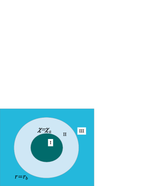
Figure 1: The 3-zone model.

First, we discuss an analytic approach to the determination of the black hole threshold. We adopt the following model, which we call the 3-zone model. See Fig. 1. We assume a flat Friedmann-Lemaitre-Robertson-Walker (FLRW) universe surrounding the overdense region (region III). The line element in the flat FLRW spacetime is applicable only for $r>r_{b}$, where $r$ is the comoving radial coordinate in the flat space. The central region (region I) undergoes expansion, maximum expansion and collapse to singularity. It is described by the closed FLRW spacetime. The line element in the closed FLRW spacetime is applicable only for $0\leq\chi<\chi_{a}$, where $\chi$ is the comoving radial coordinate in the unit 3-sphere. We need a compensating layer (region II) between regions I and III.

The Jeans criterion tells us that the pressure gradient force cannot suppress gravitational instability if and only if the free-fall time $t_{\rm ff}$ is shorter than the sound-crossing time $t_{\rm sc}$. Since we are concerned with a highly general relativistic system, we need to be precise for the application of the Jeans criterion. Here, we adopt the following criterion: if and only if the overdense region ends in singularity before a sound wave crosses its diameter from the big bang, it collapses to a black hole.

We assume an equation of state (EOS) $p=(\Gamma-1)\rho$ for simplicity. For example, $\Gamma=4/3$ corresponds to a radiation fluid. We define $\tilde{\delta}$ as the density perturbation at horizon entry in the comoving slicing. Carr [1] proposed a formula $\tilde{\delta}_{{\rm CMC},c}\simeq\Gamma-1$ and $\tilde{\delta}_{{\rm CMC},{\rm max}}\simeq 1$ in the constant-mean-curvature (CMC) slicing based on some Newtonian-like approximation. The latter is the maximum value that the perturbation can take at the horizon entry. This is transformed in the comoving slicing to $\tilde{\delta}_{c}=3\Gamma(\Gamma-1)/(3\Gamma+2),~{}~{}\tilde{\delta}_{\rm max}=3\Gamma/(3\Gamma+2)$. We can refine Carr’s formula to the following [4]:

$$\tilde{\delta}_{c}=\frac{3\Gamma}{3\Gamma+2}\sin^{2}\left(\frac{\pi\sqrt{\Gamma-1}}{3\Gamma-2}\right),\quad\tilde{\delta}_{\rm max}=\frac{3\Gamma}{3\Gamma+2}.$$ (1)

This new formula does not rely on any Newtonian-like approximation. The $\sin^{2}$ dependence comes from the spherical geometry of the overdense region and $(3\Gamma-2)$ in the denominator in the argument of $\sin^{2}$ comes from the fact that the pressure $p$ as well as the density $\rho$ appears as the source of the gravitational field in the form $(\rho+3p)$.

3 Primordial fluctuations

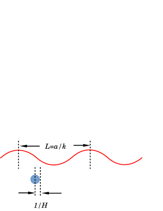
Figure 2: The CLWL solutions.

Although the 3-zone model is powerful in deriving the new analytic formula, it is by no means generic. It would be important to construct more general cosmological fluctuations. This can be done by cosmological long-wavelength (CLWL) solutions. Here, the spacetime is assumed to be smooth in the scales larger than $L=a/k$, which is much longer than the local Hubble length $H^{-1}$. Under this assumption, by gradient expansion, the exact solution is expanded in powers of $\epsilon\sim k/(aH)$. The CLWL solutions are schematically depicted in Fig. 2.

We decompose the spacetime metric in the following form:

$$ds^{2}=-\alpha^{2}dt^{2}+\psi^{4}a^{2}(t)\tilde{\gamma}_{ij}(dx^{i}+\beta^{i}dt)(dx^{j}+\beta^{j}dt),$$ (2)

and we choose $\tilde{\gamma}=\eta$, where $\tilde{\gamma}=\mbox{det}(\tilde{\gamma}_{ij})$, $\eta=\mbox{det}(\eta_{ij})$, and $\eta_{ij}$ is the metric of the 3 dimensional flat space. We call the above decomposition the cosmological conformal decomposition. According to Lyth et al. [5], we assume the spacetime locally approaches the flat FLRW form in the limit $\epsilon\to 0$. Then, the Einstein equations in $O(1)$ imply the Friedmann equation and the energy equation. We can deduce $\psi=\Psi(x^{i})+O(\epsilon^{2})$ for a perfect fluid with a barotropic EOS. $\Psi(x^{i})$ generates the solution. Thus, the different slicings are equivalent to $O(\epsilon)$.

In the following, we focus on spherically symmetric systems. Two independent approaches have been adopted for simulating PBH formation from cosmological fluctuations. The one is based on the CMC slicing and conformally flat spatial coordinates. This is adopted by Shibata and Sasaki [6]. We denote the radial coordinate in this scheme with $\varpi$. The initial conditions are given by the CLWL solutions generated by $\Psi(\varpi)$, where $\psi=\Psi(\varpi)+O(\epsilon^{2})$. The other is based on the comoving slicing and comoving threading. We denote the radial coordinate in this scheme with $r$. Polnarev and Musco [7] constructed the initial conditions as follows: the metric is assumed to approach

$$ds^{2}=-dt^{2}+a^{2}(t)\left[\frac{dr^{2}}{1-K(r)r^{2}}+r^{2}(d\theta^{2}+\sin^{2}\theta d\phi^{2})\right],$$ (3)

in the limit $\epsilon\to 0$. The exact solution is expanded in powers of $\epsilon$ and generated by $K(r)$. These solutions are called asymptotically quasi-homogeneous solutions. In fact, we can show that the CLWL solutions and the Polnarev-Musco asymptotic quasi-homogeneous solutions are equivalent with each other through the relation [9]

$$r=\Psi^{2}(\varpi)\varpi,\quad K(r)r^{2}=1-\left(1+2\displaystyle\frac{\varpi}{\Psi(\varpi)}\frac{d\Psi(\varpi)}{d\varpi}\right)^{2}.$$ (4)

We can also derive the correspondence relations between the two solutions.

4 Numerical results

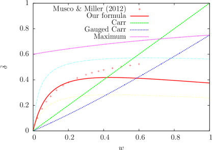
Figure 3: Carr’s formula and the new formula are plotted together with the numerical result [8] for $0.01\leq w\leq 0.6$, where $w=\Gamma-1$.

It is useful to define the amplitude of perturbation for the description of the black hole threshold. We define $\tilde{\delta}$ as the density perturbation at the horizon entry by $\tilde{\delta}:=\lim_{\epsilon\to 0}\bar{\delta}_{\rm C}(t,r_{0})\epsilon^{-2},$ where $\bar{\delta}_{\rm C}(t,r_{0})$ is the density in the comoving slicing averaged over $r_{0}$, the radius of the overdense region. $\tilde{\delta}$ can be directly calculated from $\Psi(\varpi)$ or $K(r)$. $\psi_{0}$ is the initial peak value of the curvature variable $\psi_{0}:=\Psi(0)$, which is another independent amplitude of perturbation. Thus, we can calculate the threshold value of the amplitude after we have determined the black hole threshold by numerical simulations. See [9] for the details of the numerical simulations. Our numerical results are consistent and complementary to Refs. [6, 7, 8]. We will present and interpret the numerical results below.

First we see the dependence of the threshold $\tilde{\delta}_{c}$ on the EOS. In Fig. 3, we plot Carr’s formula, the new formula (1) together with the numerical result for a Gaussian curvature profile in Musco and Miller [8]. We can see that Carr’s formula underestimates the threshold by a factor of two to ten, while the new formula agrees with the numerical result within 20 percent, although both formulas are consistent with the numerical result in the order of magnitude.

Next we see the dependence of the threshold on the initial profile. Shibata and Sasaki [6] and Polnarev and Musco [7] choose similar Gaussian-type profiles but with different parametrisations. In the former, the profile is parametrised by $\sigma$, in which the smaller the $\sigma$ is, the sharper the transition from the overdense region to the surrounding flat FLRW region becomes. In the latter, it is parametrised by $\alpha$, in which the larger the $\alpha$ is, the sharper the transition becomes. Our numerical results are plotted in Fig. 4 for $\tilde{\delta}_{c}$ and $\psi_{0,c}$. As we can see, the sharper the transition is, the larger the $\tilde{\delta}_{c}$ is but the smaller the $\psi_{0,c}$ is.

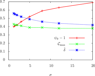
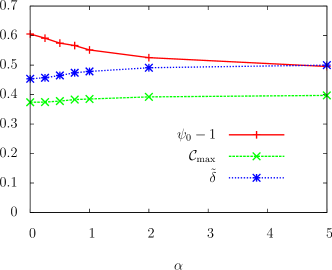
Figure 4: The threshold values $\tilde{\delta}_{c}$ and $\psi_{0,c}$ are plotted for the Gaussian-type initial profiles in the parametrisations in [6] (a) and in [7] (b).

We can naturally interpret the behaviour of $\tilde{\delta}_{c}$. To overcome larger pressure gradient force, we need stronger gravitational force and hence larger amplitude of perturbation. We can also see that the minimum value of $\tilde{\delta}_{c}$, which is realised in the gentlest transition, is close to the value given by the new formula, while the maximum value, which is realised in the sharpest transition, is close to the maximum value given by the new formula. That is, $\tilde{\delta}_{c,{\rm min}}<\tilde{\delta}_{c}<\tilde{\delta}_{c,{\rm max}}$, where

$$\tilde{\delta}_{c,{\rm min}}\simeq\frac{3\Gamma}{3\Gamma+2}\sin^{2}\left(\frac{\pi\sqrt{\Gamma-1}}{3\Gamma-2}\right),\quad\tilde{\delta}_{c,{\rm max}}\simeq\frac{3\Gamma}{3\Gamma+2}.$$ (5)

As for $\psi_{0,c}$, the behaviour is apparently opposite to that of $\tilde{\delta}_{c}$. The sharper the transition is, the smaller the $\psi_{0,c}$ is. We can interpret this by the nonlocal nature of $\psi$. In fact, $\psi$ is affected by the perturbation in the far region, which spreads even outside the local Hubble horizon, while the threshold should be determined by quasi-local dynamics within the local Hubble length. $\psi_{0,c}$ is sensitive to the environment, while $\tilde{\delta}_{c}$ is not.

5 Conclusion

We have seen that the Jeans criterion applied to the simplified toy model gives a new analytic formula for the threshold of PBH formation. For more general situations, the CLWL solutions naturally give primordial fluctuations generated by inflation. We have numerically found that the sharper the transition from the overdense region to the surrounding flat FLRW universe is, the larger the density perturbation $\tilde{\delta}_{c}$ at the threshold becomes. The new formula is supported by the numerical result in the form given by Eq. (5). The peak value of the curvature variable $\psi_{0,c}$ is subjected to the environmental effect and hence will not provide a compact criterion for the PBH formation.

This article is based on the collaboration [4, 9] with C. M. Yoo, K. Kohri, T. Nakama and Y. Koga. This work was supported by JSPS KAKENHI Grant Number 26400282.

References

- [1] B. J. Carr, “The Primordial black hole mass spectrum,” Astrophys. J. 201, 1 (1975).
- [2] B. J. Carr, K. Kohri, Y. Sendouda, and J. Yokoyama, “New cosmological constraints on primordial black holes,” Phys. Rev. D 81, 104019 (2010). [arXiv:0912.5297 [astro-ph.CO]].
- [3] M. Kopp, S. Hofmann and J. Weller, “Separate Universes Do Not Constrain Primordial Black Hole Formation,” Phys. Rev. D 83 (2011) 124025 [arXiv:1012.4369 [astro-ph.CO]].
- [4] T. Harada, C.M. Yoo and K. Kohri, Phys. Rev. D 88 (2013) 8, 084051 [Phys. Rev. D 89 (2014) 2, 029903] [arXiv:1309.4201 [astro-ph.CO]].
- [5] D. H. Lyth, K. A. Malik and M. Sasaki, “A general proof of the conservation of the curvature perturbation,” JCAP 05 (2005) 004 [astro-ph/0411220].
- [6] M. Shibata and M. Sasaki, “Black hole formation in the Friedmann universe: Formulation and computation in numerical relativity,” Phys. Rev. D 60 (1999) 084002 [gr-qc/9905064].
- [7] A. G. Polnarev and I. Musco, “Curvature profiles as initial conditions for primordial black hole formation,” Class. Quant. Grav. 24 (2007) 1405 [gr-qc/0605122].
- [8] I. Musco and J. C. Miller, “Primordial black hole formation in the early universe: critical behaviour and self-similarity,” Class. Quant. Grav. 30 (2013) 145009 [arXiv:1201.2379 [gr-qc]].
- [9] T. Harada, C.M. Yoo, T. Nakama and Y. Koga, Phys. Rev. D 91 (2015) 8, 084057 [arXiv:1503.03934 [gr-qc]].