On the Dynamics of Dengue Virus type 2 with Residence Times and Vertical Transmission

Abstract

A two-patch mathematical model of Dengue virus type 2 (DENV-2) that accounts for vectors’ vertical transmission and between patches human dispersal is introduced. Dispersal is modeled via a Lagrangian approach. A host-patch residence-times basic reproduction number is derived and conditions under which the disease dies out or persists are established. Analytical and numerical results highlight the role of hosts’ dispersal in mitigating or exacerbating disease dynamics. The framework is used to explore dengue dynamics using, as a starting point, the 2002 outbreak in the state of Colima, Mexico.

Mathematics Subject Classification: 92C60, 92D30, 93B07.

Keywords:

Vector-borne diseases, DENV-2 Asian genotype, Dengue, Residence times, Multi-Patch model, Global Stability.

1 Introduction

Dengue, a re-emerging vector-borne disease, is caused by members of the genus Flavivirus in the family Flaviviridae with four active antigenically distinct serotypes, DENV-1, DENV-2, DENV-3, and DENV-4 [22]. The pathogenicity of dengue can range from asymptomatic, mild dengue fever (DF), to dengue hemorrhagic fever (DHF), and dengue shock syndrome (DSS) [22, 34]. Although infection with a dengue serotype does not usually protect against other serotypes, it is belief that secondary infections with a heterologous serotype increase the probability of DHF and DSS [12, 33]. According to the World Health Organization, 40% of the global population is at risk for dengue infection with an estimate of 50 to 100 million infections yearly including 500,000 cases of DHF. It has been estimated that about 22,000 deaths, mostly children under 15 years of age, can be attributed to DHF [72]. In the United States, approximately 5% or more of the Key West population in Florida was exposed to dengue during the 2009-2010 outbreak [15] while the Hawaii Department of Health reported 190 cases during the 2015 outbreak on Oahu, the first outbreak since 2011. Since dengue is not endemic in Hawaii, health authorities have suggested that the recent outbreak may have been started by infected visitors [57]. Dengue is highly prevalent and endemic in Southeast Asia, which has experienced a 70% increase in cases since 2004 [40]; Mexico, also an endemic country, reported during the 2002 outbreak over a million cases of DF and more than 17,000 cases of DHF[32, 50]. Dengue is transmitted primarily by the vector Ae. aegypti, which is now found in most countries in the tropics and sub-tropics [35, 59]. The secondary vector, Ae. albopictus, has a range reaching farther north than Ae. aegypti with eggs better adapted to subfreezing temperatures [36, 50]. Differences in susceptibility and transmission of dengue infection [3, 39, 70] raise the possibility that some serotypes are either more successful at invading a host population, or more pathogenic, or both[41]. DENV-2 is the most associated with dengue outbreaks involving DHF and DSS cases [49, 61, 66, 74], followed by DENV-1 and DENV-3 viruses [5, 35, 49]. While infection with any of the four dengue serotypes could lead to DHF, the rapid displacement of DENV-2 American by DENV-2 Asian genotype has been linked to major outbreaks with DHF cases in Cuba, Jamaica, Venezuela, Colombia, Brazil, Peru and Mexico [74, 61, 66, 49, 42, 60]. A possible mechanism involved in the dispersal and persistence of DENV-2 in nature is vertical transmission (transovarial transmission) via Ae. aegypti. Prior studies were unsuccessful in demonstrating vertical transmission via Ae. aegypti [62]. However, the use of advances in molecular biology has shown that vertical transmission involving Ae. aegypti and Ae. albopictus is possible in captivity and in the wild [3, 10, 16, 31, 63]. Thus, assessing transmission dynamics and pathogenicity between the DENV-2 American and Asian genotypes’ differences is one of the priorities associated with the study of the epidemiology of dengue. In short, dengue has an increasing recurrent presence putting a larger percentage of the global population at risk of dengue infection, a situation that has become the norm due to the growth of travel and tourism between endemic and non-endemic regions. The aim of this work is to better understand the impact of human mobility on dengue disease transmission, its impact on dengue dynamics, and the use mobility based strategies, an standard control measures, in reducing the prevalence of dengue infections .

Mathematical models describing the dynamics of interaction between host and vector go back to Ross [64], Lotka [44] and MacDonald [45]; first used to study vector-host dynamics in the context of Malaria [11, 30, 65]. Variations of such framework have been applied to dengue ( for a review see [67]). Further applications of modeling variations in the context of Malaria include,[27, 48, 53, 55] and in the context of dengue [13, 20, 30, 51, 56].

The potential role of vertical transmission in dengue endemic regions or in fluctuating environments has been explored in [1, 26, 56]. The role in the displacement of DENV-2 American via DENV-2 Asian vertical transmission has also been addressed [51]. The role of host movement has also been explored in the context of dengue [2] in a formulation that does not account for the the effective population size. In this paper, the role of vertical transmission and movement via residence times are explored via a two-patch model involving non-mobile vectors and mobile hosts. This paper is organized as follows: The derivation of the model is presented in Section 2; Analytical results are collected in Section 3; The results of numerical simulations are collected in Section 4; Section 5 explores the possible role of movement on joint dynamics of dengue in Colima and Manzanillo in the presence of host mobility; Concluding remarks are collected in Section 6.

2 Derivation of the model

A single patch model is derived and embedded into a two-patch model via a residence-times matrix in order to study the impact of host mobility on dengue disease dynamics. Conditions for dengue eradication and persistence in the population are computed.

2.1 Single patch model

We consider a population of host composed of susceptible ($S_{h}$), exposed ($E_{h}$), infectious ($I_{h}$) and recovered $(R_{h})$ individuals interacting with a vector population composed of susceptible ($S_{v}$), exposed ($E_{v}$) and infected ($I_{v}$) vectors. The dynamics of dengue follows an $SEIR$ structure for the host population and an $SEI$ type for the vector population. The birth rate for the host population is $\mu_{h}$, assumed to be equal to the death rate, that is, hosts’ demographic differentials are conveniently ignored, that is, the host population is assumed to be constant. Susceptible hosts are infected, by infectious mosquitoes, at the rate $a\beta_{vh}\frac{I_{v}}{N_{h}}$ where $a$ is the biting rate and $\beta_{vh}$ is the infectiousness of human to mosquitoes. The exposed population develops symptoms becoming infectious at the rate $\nu_{h}$. Infectious individuals recover at the per-capita rate $\gamma$. Susceptible mosquitoes become infected, via interactions with infectious hosts, at the rate $a\beta_{hv}\frac{I_{h}}{N_{h}}$. Recent studies place significant importance to the connection between DENV-2 and DHF cases [19, 25, 49, 61, 66, 74] and on DENV-2 vertical transmission [47]. Hence, it is assumed that a fraction $q$ of the mosquitoes are “born” infected entering directly the infectious class. The natural per-capita vector mortality is $\mu_{v}$.

The model describing the dynamics of DENV-2 is given by the following system of differential equations:

$$\left\{\begin{array}[]{llll}\dot{S}_{h}=\mu_{h}N_{h}-a\beta_{vh}S_{h}\frac{I_{v}}{N_{h}}-\mu_{h}S_{h}\\ \dot{E}_{h}=\beta_{vh}S_{h}\frac{I_{v}}{N_{h}}-(\mu_{h}+\nu_{h})E_{h}\\ \dot{I}_{h}=\nu_{h}E_{h}-(\mu_{h}+\gamma_{h})I_{h}\\ \dot{R}_{h}=\gamma_{h}I_{h}-\mu_{h}R_{h}\\ \dot{S}_{v}=\mu_{v}(N_{v}-qI_{v})-a\beta_{hv}S_{v}\frac{I_{h}}{N_{h}}-\mu_{v}S_{v}\\ \dot{E}_{v}=a\beta_{hv}S_{v}\frac{I_{h}}{N_{h}}-(\nu_{v}+\mu_{v})E_{v}\\ \dot{I}_{v}=\nu_{v}E_{v}+q\mu_{v}I_{v}-\mu_{v}I_{v}\end{array}\right.$$ (1)

In the absence of selection, that is, differences in birth and death rate and in the absence of vertical transmission, Model (1) turns out to be isomorphic to model considered by Chowell et al in [18]. Model (1) is well defined supporting a sharp threshold property, namely, the disease dies out if the basic reproduction number $\mathcal{R}_{0}$ is less than unity, persisting whenever $\mathcal{R}_{0}>1$ where

$$\mathcal{R}_{0}^{2}=\frac{a^{2}\beta_{hv}\beta_{vh}N_{v}\nu_{h}\nu_{v}}{(1-q)N_{h}(\mu_{h}+\nu_{h})(\mu_{h}+\gamma_{h})(\mu_{v}+\nu_{v})\mu_{v}}.$$

2.2 Heterogeneity through virtual dispersal

The single patch model is the building block for the two-patch model used in this study. Within each patch, in the absence of host mobility, dengue dynamics are modeled via System 1. A metapopulation approach, an Eulerian perspective, is most often applied to the study of vector-borne diseases involving host mobility ([2, 4, 28]). Here, a Lagrangian approach is used instead to model the movement of individuals between patches (see [7, 8]). It is assumed that vectors don’t move between patches since vecors Ae. aegypti and Ae. albopictus do not travel more than few tens of meters over their lifetime [2, 58]; moving 400-600 meters at most [9, 54], respectively. In short, we neglect vector’s dispersal, which fits well the simulations involving two cities in the state of Colima, Mexico.

The host resident of Patch 1, population size $N_{h,1}$, spends, on average, $p_{11}$ proportion of its time in their own Patch 1 and $p_{12}$ proportion of its time visiting Patch 2. Residents of Patch 2, population of size $N_{h,2}$, spend $p_{22}$ proportion of their time in Patch 2 while spending $p_{21}=1-p_{22}$ visiting Patch 1. Thus, at time $t$, the effective population in Patch 1 is $p_{11}N_{h,1}+p_{21}N_{h,2}$ and the effective population in Patch 2 is $p_{12}N_{h,1}+p_{22}N_{h,2}$. The susceptible population of Patch 1 ($S_{1}$) could be infected by a vector in either Patch 1 ($I_{v,1}$) or Patch 2 by ($I_{v,2}$). Thus, the dynamics of the susceptible population in Patch 1 are given by

$$\dot{S}_{h,1}=\mu_{h}N_{h,1}-a_{1}\beta_{vh}p_{11}S_{h,1}\frac{I_{v,1}}{p_{11}N_{h,1}+p_{21}N_{h,2}}-a_{2}\beta_{vh}p_{12}S_{h,1}\frac{I_{v,2}}{p_{12}N_{h,1}+p_{22}N_{h,2}}-\mu_{h}S_{h,1}.$$ (2)

And so, the effective infectious population in Patch 1 is $p_{11}I_{h,1}+p_{21}I_{h,2}$ and, consequently, the proportion of infectious individuals in Patch 1, is

$$\frac{p_{11}I_{h,1}+p_{21}I_{h,2}}{p_{11}N_{h,1}+p_{21}N_{h,2}}.$$

The dynamics of susceptible mosquitoes in Patch 1 are modeled as follows:

$$\dot{S}_{v,1}=\mu_{v}(N_{v,i}-qI_{v,i})-a_{1}\beta_{hv}S_{v,1}\frac{p_{11}I_{h,1}+p_{21}I_{h,2}}{p_{11}N_{h,1}+p_{21}N_{h,2}}-\mu_{v}S_{v,1}.$$ (3)

The complete dynamics of DENV-2, with the host moving between patches, is given by the following system,

$$\left\{\begin{array}[]{llll}\dot{S}_{h,i}=\mu_{h}N_{h,i}-\beta_{vh}S_{h,i}\sum_{j=1}^{2}a_{j}p_{ij}\frac{I_{v,j}}{p_{1j}N_{h,1}+p_{2j}N_{h,2}}-\mu_{h}S_{h,i},\\ \dot{E}_{h,i}=\beta_{vh}S_{h,i}\sum_{j=1}^{2}a_{j}p_{ij}\frac{I_{v,j}}{p_{1j}N_{h,1}+p_{2j}N_{h,2}}-(\mu_{h}+\nu_{h})E_{h,i},\\ \dot{I}_{h,i}=\nu_{h}E_{h,i}-(\mu_{h}+\gamma_{i})I_{h,i},\\ \dot{R}_{h,i}=\gamma_{i}I_{h,i}-\mu_{h}R_{h,i},\\ \dot{S}_{v,i}=\mu_{v}(N_{v,i}-qI_{v,i})-a_{i}\beta_{hv}S_{v,i}\frac{\sum_{j=1}^{2}p_{ji}I_{h,j}}{\sum_{k=1}^{2}p_{ki}N_{h,k}}-\mu_{v}S_{v,i},\\ \dot{E}_{v,i}=a_{i}\beta_{hv}S_{v,i}\frac{\sum_{j=1}^{2}p_{ji}I_{h,j}}{\sum_{k=1}^{2}p_{ki}N_{h,k}}-(\mu_{v}+\nu_{v})E_{v,i},\\ \dot{I}_{v,i}=\nu_{v}E_{h,i}+q\mu_{v}I_{v,i}-\mu_{v}I_{v,i},i=1,2.\end{array}\right.$$ (4)

Since the total populations of hosts and vectors are constant in each patch, System (4) has the same qualitative dynamics as,

$$\left\{\begin{array}[]{llll}\dot{S}_{h,i}=\mu_{h}N_{h,i}-\beta_{vh}S_{h,i}\sum_{j=1}^{2}a_{j}p_{ij}\frac{I_{v,j}}{p_{1j}N_{h,1}+p_{2j}N_{h,2}}-\mu_{h}S_{h,i},\\ \dot{E}_{h,i}=\beta_{vh}S_{h,i}\sum_{j=1}^{2}a_{j}p_{ij}\frac{I_{v,j}}{p_{1j}N_{h,1}+p_{2j}N_{h,2}}-(\mu_{h}+\nu_{h})E_{h,i},\\ \dot{I}_{h,i}=\nu_{h}E_{h,i}-(\mu_{h}+\gamma_{i})I_{h,i},\\ \dot{E}_{v,i}=a_{i}\beta_{hv}(N_{v,i}-E_{v,i}-I_{v,i})\frac{\sum_{j=1}^{2}p_{ji}I_{h,j}}{\sum_{k=1}^{2}p_{ki}N_{h,k}}-(\mu_{v}+\nu_{v})E_{v,i},\\ \dot{I}_{v,i}=\nu_{v}E_{h,i}-(1-q)\mu_{v}I_{v,i}.\end{array}\right.$$ (5)

Table 1: Description of the parameters used in System (5).

Parameters	Description
$\beta_{vh}$	Infectiousness of human to mosquitoes
$\beta_{hv}$	Infectiousness of mosquitoes to humans
$a_{i}$	Biting rate in Patch $i$
$\mu_{h}$	Humans’ birth and death rate
$\nu_{h}$	Humans’ incubation rate
$\gamma_{i}$	Recovery rate in Patch $i$
$p_{ij}$	Proportion of time residents of Patch $i$ spend in Patch $j$
$\mu_{v}$	Vectors’ natural birth and mortality rate
$\nu_{v}$	Vectors’ incubation rate
$q$	Proportion of mosquitoes infected through transovarial transmission

The parameters of Model 5 are described in Table 1.

We now show that the model is biologically well posed.

Lemma 2.1.

The set

$$\Omega=\{(S_{h,i},E_{h,i},I_{h,i},E_{v,i},I_{v,i})\in\mathbb{R}^{6}_{+}\quad\mid\quad S_{h,i}+E_{h,i}+I_{h,i}\leq N_{h,i},\;E_{v,i}+I_{v,i}\leq N_{v,i}\}$$

is a compact positively invariant for the System (5).

Proof.

The positive orthant is clearly positively invariant. Since the host population is constant, then the inequality $S_{i}+E_{i}+I_{i}\leq N_{h,i}$ is always satisfied. We have

$$\dot{E}_{v,i}+\dot{I}_{v,i}\mid_{E_{h,i}=N_{v,i}} = -a_{i}\beta_{hv}I_{v,i}\frac{\sum_{j=1}^{2}p_{ji}I_{h,j}}{\sum_{k=1}^{2}p_{ki}N_{h,k}}-(\mu_{v}+\nu_{v})N_{v,i}$$

$$\leq 0$$

Hence, $E_{v,i}+I_{v,i}\leq N_{v,i}$ and the set $\Omega$, an intersection of positively invariant sets ( $\mathbb{R}^{7}_{+}$, $\{S_{i}+E_{i}+I_{i}\leq N_{h,i}\}$ and $\{E_{v,i}+I_{v,i}\leq N_{v,i}\}$), is positively invariant; the set is a compact set.
∎

3 Equilibria and stability analysis

This section characterizes the equilibrium dynamics of Model (5).

3.1 The disease free equilibrium and the basic reproduction number

The disease free equilibrium is

$$E_{0}=(N_{h,1},N_{h,2},\textbf{0}_{\mathbb{R}^{8}}),$$

which is used to compute the basic reproduction number via the next generation method [24, 71]. The basic reproduction number $\mathcal{R}_{0}$ is defined by the expression (See Appendix A, for details), $\mathcal{R}_{0}^{2}=\rho(M_{vh}M_{hv})$, that is, the spectral radius of the matrix of $M_{vh}M_{hv}$, where

$$M_{vh}=\left(\begin{array}[]{cc}\frac{a_{1}\beta_{vh}p_{11}N_{h,1}\nu_{v}}{(p_{11}N_{h,1}+p_{21}N_{h,2})(\mu_{v}+\nu_{v})(1-q)\mu_{v}}&\frac{a_{2}\beta_{vh}p_{12}N_{h,1}\nu_{v}}{(p_{12}N_{h,1}+p_{22}N_{h,2})(\mu_{v}+\nu_{v})(1-q)\mu_{v}}\\ \frac{a_{1}\beta_{vh}p_{21}N_{h,2}\nu_{v}}{(p_{11}N_{h,1}+p_{21}N_{h,2})(\mu_{v}+\nu_{v})(1-q)\mu_{v}}&\frac{a_{2}\beta_{vh}p_{22}N_{h,2}\nu_{v}}{(p_{12}N_{h,1}+p_{22}N_{h,2})(\mu_{v}+\nu_{v})(1-q)\mu_{v}}\end{array}\right)$$

and

$$M_{hv}=\left(\begin{array}[]{cc}\frac{a_{1}\beta_{hv}p_{11}N_{v,1}\nu_{h}}{(p_{11}N_{h,1}+p_{21}N_{h,2})(\mu_{h}+\nu_{h})(\mu_{h}+\gamma_{1})}&\frac{a_{1}\beta_{hv}p_{21}N_{v,1}\nu_{h}}{(p_{11}N_{h,1}+p_{21}N_{h,2})(\mu_{h}+\nu_{h})(\mu_{h}+\gamma_{2})}\\ \frac{a_{2}\beta_{hv}p_{12}N_{v,2}\nu_{h}}{(p_{12}N_{h,1}+p_{22}N_{h,2})(\mu_{h}+\nu_{h})(\mu_{h}+\gamma_{1})}&\frac{a_{2}\beta_{hv}p_{22}N_{v,2}\nu_{h}}{(p_{12}N_{h,1}+p_{22}N_{h,2})(\mu_{h}+\nu_{h})(\mu_{h}+\gamma_{2})}\end{array}\right).$$

The matrix $\left(\begin{array}[]{cc}0&M_{vh}\\ M_{hv}&0\end{array}\right)$ is called the host-vector network configuration [38]. The result of local asymptotic stability if $\mathcal{R}_{0}^{2}<1$ and instability if $\mathcal{R}_{0}^{2}>1$ has been established in [71]. The following theorem gives the global result of the DFE.

Theorem 3.1.

If $\mathcal{R}_{0}^{2}\leq 1$, the DFE is globally asymptotically stable in the nonnegative orthant. If $\mathcal{R}_{0}^{2}>1$, the DFE is unstable.

Proof.

We use the comparison theorem [68] to prove the GAS of the DFE. Since $S_{h,i}\leq N_{h,i}$ and $S_{v,i}\leq N_{v,i}$, we have that,

$$\dot{E}_{h,i}\leq\beta_{vh}N_{h,i}\sum_{j=1}^{2}a_{j}p_{ij}\frac{I_{v,j}}{p_{1j}N_{h,1}+p_{2j}N_{h,2}}-(\mu_{h}+\nu_{h})E_{h,i}$$ (6)

and

$$\dot{E}_{v,i}\leq a_{i}\beta_{hv}N_{v,i}\frac{\sum_{j=1}^{2}p_{ji}I_{h,j}}{\sum_{k=1}^{2}p_{ki}N_{h,k}}-(\mu_{v}+\nu_{v})E_{v,i}.$$ (7)

We define an auxiliary system via the right hand side of Equations (6)-(7) and the infected compartments of Equation (5) as follows:

$$\left(\begin{array}[]{c}\dot{E}_{h,i}\\ \dot{E}_{v,i}\\ \dot{I}_{h,i}\\ \dot{I}_{v,i}\end{array}\right) = \left(\begin{array}[]{c}\beta_{vh}N_{h,i}\sum_{j=1}^{2}a_{j}p_{ij}\frac{I_{v,j}}{p_{1j}N_{h,1}+p_{2j}N_{h,2}}-(\mu_{h}+\nu_{h})E_{h,i}\\ a_{i}\beta_{hv}N_{v,i}\frac{\sum_{j=1}^{2}p_{ji}I_{h,j}}{\sum_{k=1}^{2}p_{ki}N_{h,k}}-(\mu_{v}+\nu_{v})E_{v,i}\\ \nu_{h}E_{h,i}-(\mu_{h}+\gamma_{i})I_{h,i}\\ \nu_{v}E_{h,i}-(1-q)\mu_{v}I_{v,i}\end{array}\right)$$ (16)

$$= (F+V)\left(\begin{array}[]{c}E_{h,i}\\ E_{v,i}\\ I_{h,i}\\ I_{v,i}\end{array}\right);$$ (21)

where the matrices $F$ and $V$ in (16) were just generated using the next generation method. System (16) is linear and its dynamics is well known. Since $V$ is a Metzler matrix and $F$ a nonnegative matrix ([6]), then

$$\rho(-FV^{-1})<1\iff\alpha(F+V)<0$$

where $\alpha(F+V)$ is the stability modulus of $F+V$. Thus, if $\mathcal{R}_{0}=\rho(-FV^{-1})<1$, all the eigenvalues of $F+V$ are negative. Hence, the nonnegative solutions of (16) are such that

$$\lim_{t\to\infty}E_{h,i}=\lim_{t\to\infty}E_{v,i}=0\quad\text{and}\quad\lim_{t\to\infty}I_{h,i}=\lim_{t\to\infty}I_{v,i}=0$$

Since, all the variables in System (5) are nonnegative, the use of a comparison theorem [68] leads to,

$$\lim_{t\to\infty}E_{h,i}=\lim_{t\to\infty}E_{v,i}=0\quad\text{and}\quad\lim_{t\to\infty}I_{h,i}=\lim_{t\to\infty}I_{v,i}=0,\quad i=1,2.$$

Therefore, by using the asymptotic theory of autonomous systems [14], System (5) has the qualitative dynamics of the following limit system:

$$\dot{S}_{h,i}=\mu_{h}N_{h,i}-\mu_{h}S_{h,i}$$

for which the equilibrium $(N_{h,1},N_{h,2})$ is globally asymptotically stable. If $\mathcal{R}_{0}>1$, the instability of the DFE follows from [24, 71]. ∎

Theorem 3.2.

If $\mathcal{R}_{0}>1$, System (5) is uniformly persistent, that is, it exists $\eta>0$ such that $\displaystyle\liminf_{t\to\infty}\{S_{h,i},E_{h,i},I_{h,i},E_{v,i},I_{v,i}\}>\eta$ for any initial conditions satisfying $S_{h,i}(0)>0$, $E_{h,i}(0)>0,$ $I_{h,i}(0)>0$, $E_{v,i}(0)>0$ and $I_{v,i}(0)>0$ for $i=1,2$.

Proof.

Let $X=\Omega$, $x=(S_{h,1},S_{h,2},E_{h,1},E_{h,2},E_{v,1},E_{v,2},I_{h,1},I_{h,2},I_{v,1},I_{v,2})$ and $X_{0}=\{x\in X\;\mid\;I_{v,1}+I_{v,2}>0\}$ Hence, $\partial X_{0}=X\backslash X_{0}=\{x\in X\;\mid\;I_{v,1}=I_{v,2}=0\}$. Let $\phi_{t}$ be semi-flow induced by the solutions of (5) and $M_{\partial}=\{x\in\partial X_{0}\;\mid\;\phi_{t}x\in\partial X_{0},t\geq 0\}$. By Lemma 2.1, we have $\phi_{t}X_{0}\subset X_{0}$ and $\phi_{t}$ is bounded in $X_{0}$. Therefore a global attractor for $\phi_{t}$ exists . The DFE is the unique equilibrium on the manifold $\partial X_{0}$ and is GAS on $\partial X_{0}$. Moreover $\cup_{x\in M_{\partial}}\omega(x)=\{E_{0}\}$ and no subset of $M$ forms a cycle in $\partial X_{0}$. Finally since the DFE is unstable on $X_{0}$ if $\mathcal{R}_{0}>1$, we deduce that System (5) is uniformly persistent by using a result from [75] (Theorem 1.3.1 and Remark 1.3.1). ∎

Theorem 3.3.

Whenever the host-vector configuration is irreducible and $\mathcal{R}_{0}^{2}>1$, System (5) has a unique endemic equilibrium.

Proof.

We will use a result by Hethcote and Thieme [37] to prove the uniqueness of the endemic equilibrium. An endemic equilibrium $(\bar{S}_{h,1},\bar{S}_{h,2},\bar{E}_{h,1},\bar{E}_{h,2},\bar{E}_{v,1},\bar{E}_{v,2},\bar{I}_{h,1},\bar{I}_{h,2},\bar{I}_{v,1},\bar{I}_{v,2})$ satisfies:

$$\left\{\begin{array}[]{llll}\mu_{h}N_{h,i}=\beta_{vh}\bar{S}_{h,i}\sum_{j=1}^{2}a_{j}p_{ij}\frac{\bar{I}_{v,j}}{p_{1j}N_{h,1}+p_{2j}N_{h,2}}+\mu_{h}\bar{S}_{h,i},\\ (\mu_{h}+\nu_{h})\bar{E}_{h,i}=\beta_{vh}\bar{S}_{h,i}\sum_{j=1}^{2}a_{j}p_{ij}\frac{\bar{I}_{v,j}}{p_{1j}N_{h,1}+p_{2j}N_{h,2}},\\ \nu_{h}\bar{E}_{h,i}=(\mu_{h}+\gamma_{i})\bar{I}_{h,i},\\ (\mu_{v}+\nu_{v})\bar{E}_{v,i}=a_{i}\beta_{hv}(N_{v,i}-\bar{E}_{v,i}-\bar{I}_{v,i})\frac{\sum_{j=1}^{2}p_{ji}\bar{I}_{h,j}}{\sum_{k=1}^{2}p_{ki}N_{h,k}},\\ (1-q)\mu_{v}I_{v,i}=\nu_{v}E_{v,i}.\end{array}\right.$$ (22)

The first equation of (22) implies that

$$\bar{S}_{h,i}=\frac{\mu_{h}N_{h,i}}{\beta_{vh}\sum_{j=1}^{2}a_{j}p_{ij}\frac{\bar{I}_{v,j}}{p_{1j}N_{h,1}+p_{2j}N_{h,2}}+\mu_{h}}.$$

Hence, we deduce that, from System (22), that

$$\left\{\begin{array}[]{llll}\bar{E}_{h,i}=\frac{\beta_{vh}}{\mu_{h}+\nu_{h}}\frac{\mu_{h}N_{h,i}}{\beta_{vh}\sum_{j=1}^{2}a_{j}p_{ij}\frac{\bar{I}_{v,j}}{p_{1j}N_{h,1}+p_{2j}N_{h,2}}+\mu_{h}}\sum_{j=1}^{2}a_{j}p_{ij}\frac{\bar{I}_{v,j}}{p_{1j}N_{h,1}+p_{2j}N_{h,2}},\\ \bar{I}_{h,i}=\frac{\nu_{h}}{\mu_{h}+\gamma_{i}}\bar{E}_{h,i},\\ \bar{E}_{v,i}=\frac{a_{i}\beta_{hv}}{\mu_{v}+\nu_{v}}(N_{v,i}-\bar{E}_{v,i}-\bar{I}_{v,i})\frac{\sum_{j=1}^{2}p_{ji}\bar{I}_{h,j}}{\sum_{k=1}^{2}p_{ki}N_{h,k}},\\ \bar{I}_{v,i}=\frac{\nu_{v}}{(1-q)\mu_{v}}\bar{E}_{v,i}.\end{array}\right.$$ (23)

Let

$$F(x)=\left(\begin{array}[]{c}\frac{\beta_{vh}\nu_{v}}{(1-q)(\mu_{h}+\nu_{h})\mu_{v}}\frac{\mu_{h}N_{h,1}}{\beta_{vh}\sum_{j=1}^{2}\frac{a_{j}p_{1j}\nu_{v}}{(1-q)\mu_{v}}\frac{\bar{E}_{v,j}}{p_{1j}N_{h,1}+p_{2j}N_{h,2}}+\mu_{h}}\sum_{j=1}^{2}a_{j}p_{1j}\frac{\bar{E}_{v,j}}{p_{1j}N_{h,1}+p_{2j}N_{h,2}}\\ \frac{\beta_{vh}\nu_{v}}{(1-q)(\mu_{h}+\nu_{h})\mu_{v}}\frac{\mu_{h}N_{h,2}}{\beta_{vh}\sum_{j=1}^{2}\frac{a_{j}p_{2j}\nu_{v}}{(1-q)\mu_{v}}\frac{\bar{E}_{v,j}}{p_{1j}N_{h,1}+p_{2j}N_{h,2}}+\mu_{h}}\sum_{j=1}^{2}a_{j}p_{2j}\frac{\bar{E}_{v,j}}{p_{1j}N_{h,1}+p_{2j}N_{h,2}}\\ \frac{a_{1}\beta_{hv}\nu_{h}}{(\mu_{v}+\nu_{v})(\mu_{h}+\gamma_{1})}(N_{v,1}-\bar{E}_{v,1}-\frac{\nu_{v}}{(1-q)\mu_{v}}\bar{E}_{v,1})\frac{\sum_{j=1}^{2}p_{j1}\bar{E}_{h,j}}{\sum_{k=1}^{2}p_{k1}N_{h,k}}\\ \frac{a_{2}\beta_{hv}\nu_{h}}{(\mu_{v}+\nu_{v})(\mu_{h}+\gamma_{2})}(N_{v,2}-\bar{E}_{v,2}-\frac{\nu_{v}}{(1-q)\mu_{v}}\bar{E}_{v,2})\frac{\sum_{j=1}^{2}p_{j2}\bar{E}_{h,j}}{\sum_{k=1}^{2}p_{k2}N_{h,k}}\par\par\end{array}\right)$$

where $x=(\bar{E}_{h,1},\bar{E}_{h,2},\bar{E}_{v,1},\bar{E}_{v,2},\bar{I}_{h,1},\bar{I}_{h,2})$. The function $F(x)$ is continuous, bounded, differentiable and $F(0_{\mathbb{R}^{6}})=0_{\mathbb{R}^{6}}$. The function $F$ is monotone if the corresponding Jacobian matrix is Metzler, i.e all off-diagonal entries are nonnegative. We have:

$$DF(x)=\left(\begin{array}[]{cc}\begin{array}[]{cc}0&0\\ 0&0\end{array}&\tilde{M}_{vh}(x)\\ \tilde{M}_{hv}(x)&\begin{array}[]{cc}-a_{1}\beta_{hv}\left(1+\frac{\nu_{v}}{(1-p)\mu_{v}}\right)\frac{\sum_{k=1}^{2}\frac{p_{k1}\nu_{h}E_{h,k}}{\mu_{h}+\gamma_{k}}}{p_{11}N_{h,1}+p_{21}N_{h,2}}&0\\ 0&-a_{2}\beta_{hv}\left(1+\frac{\nu_{v}}{(1-p)\mu_{v}}\right)\frac{\sum_{k=1}^{2}\frac{p_{k2}\nu_{h}E_{h,k}}{\mu_{h}+\gamma_{k}}}{p_{12}N_{h,1}+p_{22}N_{h,2}}\end{array}\par\end{array}\right)$$

where

$$\tilde{m}_{vh}^{ij}(x) = \frac{\beta_{vh}^{2}\mu_{h}\nu_{v}a_{j}p_{ij}N_{h,j}}{(1-p)\mu_{v}(\mu_{h}+\nu_{h})\sum_{k=1}^{2}p_{kj}N_{h,k}}\frac{1}{\frac{\beta_{vh}}{(1-q)\mu_{v}}\sum_{k=1}^{2}\frac{a_{k}p_{jk}E_{v,k}}{p_{1k}N_{h,1}+p_{2k}N_{h,2}}+\mu_{h}}\left[\frac{}{}1-\right.$$ (24)

$$\left.\frac{\frac{\beta_{vh}}{(1-q)\mu_{v}}\sum_{k=1}^{2}\frac{a_{k}p_{jk}E_{v,k}}{p_{1k}N_{h,1}+p_{2k}N_{h,2}}}{\frac{\beta_{vh}}{(1-q)\mu_{v}}\sum_{k=1}^{2}\frac{a_{k}p_{jk}E_{v,k}}{p_{1k}N_{h,1}+p_{2k}N_{h,2}}+\mu_{h}}\right]$$

and

$$\tilde{m}_{hv}^{ij}(x)=a_{i}\beta_{hv}\left(N_{v,i}-E_{v,i}-\frac{\nu_{v}E_{v,i}}{(1-p)\mu_{v}}\right)\frac{\nu_{h}p_{ji}}{(\mu_{h}+\gamma_{i})\sum_{k=1}^{2}p_{ki}N_{h,k}}.$$

Since, $\tilde{m}_{vh}^{ij}\geq 0$ and $\tilde{m}_{hv}^{ij}\geq 0$ for all $i,j=1,2$, hence all off diagonal entries of the Jacobian matrix are nonnegative and so, the function $F(x)$ is monotone, moreover,

$$DF(0_{\mathbb{R}^{4}})=\left(\begin{array}[]{cc}\begin{array}[]{cc}0&0\\ 0&0\end{array}&\tilde{M}_{vh}(0)\\ \tilde{M}_{hv}(0)&\begin{array}[]{cc}0&0\\ 0&0\end{array}\end{array}\right).$$

This matrix is irreducible whenever $\tilde{M}_{vh}(0)\tilde{M}_{hv}(0)$ and $\tilde{M}_{hv}(0)\tilde{M}_{vh}(0)$ are irreducible. The latter is guaranteed since $M_{vh}M_{hv}$ and $M_{hv}M_{vh}$ (from the next generation matrix) are both irreducible. Hence, an application of Theorem 2.1 in [37] implies that Model (23) has a unique positive fixed point if and only if $\rho(DF(0_{\mathbb{R}^{4}}))=\mathcal{R}_{0}>1$, or equivalently $\mathcal{R}_{0}^{2}>1$. ∎

If the host-vector configuration is not irreducible, that is, the graphs associated with the matrices $M_{vh}M_{hv}$ and $M_{hv}M_{vh}$ are not strongly connected, the dynamics of the disease within patches are either somehow independent or System (5) exhibits boundary equilibria. It is worthwhile noting that the irreducibility of residence times matrix $\mathbb{P}$ does not imply the irreducibility of $M_{vh}M_{hv}$ and $M_{hv}M_{vh}$. Since the epidemiological and entomological parameters are all positive, the reducibility of the host-vector configuration happens only on the three following cases: (i) If the two patches are isolated, i.e: $p_{12}=p_{21}=0$; (ii) residents of Patch 1 spend all their time in Patch 2 and residents of Patch 2 spend all their time in their own patch, i.e: $p_{12}=1$ and $p_{21}=0$; and (iii) the opposite scenario of (ii).

4 Simulations

Simulations are carried out in order to highlight the effects of residence times on disease dynamics. The simulations have a dual goal, first, to illustrate the theoretical results of this manuscript and secondly to illustrate the impact of host mobility across high and low-risk dengue areas.

The basic reproduction reproduction number $\mathcal{R}_{0}(\mathbb{P})$ is a function of the residence times matrix $\mathbb{P}$. Simulation baseline values, except for those involving the entries of $\mathbb{P}$ are as follows:

$$\beta_{hv}=0.5(0.001-0.54),\;\beta_{vh}=0.41(0.3-0.9),\;\frac{1}{\mu_{v}}=20(10-30)\;\textrm{days},\;a_{1}=0.95\;\textrm{day}^{-1},a_{2}=0.8\;\textrm{day}^{-1},$$

$$\frac{1}{\mu_{h}}=60\times 365\;\textrm{days},\;\frac{1}{\gamma_{1}}=7\;\textrm{days},\;\frac{1}{\gamma_{2}}=6\;\textrm{days},\;\frac{1}{\nu_{h}}=5\;\textrm{days},\;\frac{1}{\nu_{v}}=7\;\textrm{days}.$$

The values of the parameters $\nu_{h}$ and $\nu_{v}$ are taken from [1, 2]. The infectiousness parameters ($\beta_{hv}$ and $\beta_{vh}$) and vector’s natural mortality rate are taken from [17]. Host and vector population are

$$N_{h,1}=400,000\;N_{h,2}=300,000\;N_{v,1}=35,000,\;N_{v,2}=30,000$$

Patch 1 is the high-risk and Patch 2 is the low-risk and so, it is assumed that $a_{1}>a_{2}$. Figure 1 represents the dynamics of Patch 1 (Fig 1(a)) and Patch 2 (Fig 1(b)) infected hosts while Fig 2 collects the vector dynamics in both patches. Since Patch 1 is high-risk, the number of infected host should decrease as $p_{12}$ increases; see Fig 1(a). Figure 1(b) shows the Patch 2 infected host population, which it is decreasing, as $p_{21}$ and $p_{12}$ increase. Disease prevalence among Patch 2 residents remains very small when compared to that in Patch 1. In Fig 2, Patch 1 (Fig 2(a)) and Patch 2 (Fig 2(b)) vector dynamics are seen to follow the hosts’ endemicity pattern.

For all the different values of $p_{ij}$ chosen in Fig 1 and Fig 2, the host-vector configuration matrix

$$M=\left(\begin{array}[]{cc}0&M_{vh}\\ M_{vh}&0\end{array}\right)$$

or equivalently, the products $M_{hv}M_{vh}$ and $M_{vh}M_{hv}$, are irreducible. Moreover the basic reproduction number $\mathcal{R}_{0}$ is greater than one, hence the the disease is, in both patches, at an endemic level.

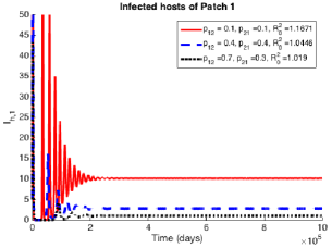
(a) The level of infected host in Patch 1 seems to decrease as $p_{12}$ increases (and hence $p_{11}$ decreases).

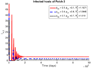
(b) The level of infected host in Patch 2 seems to decrease with respect to $p_{22}$.

Figure 1: Dynamics of $I_{h,1}$ and $I_{h,2}$ for different values of $p_{ij}$.

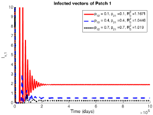
(a) Asymptotically, the level of infected vectors in Patch 1 seems to decrease as $p_{12}$ increases (and hence $p_{11}$ decreases).

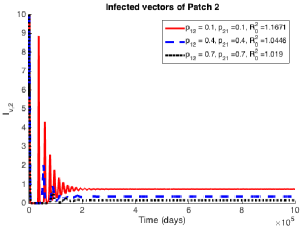
(b) Asymptotically, the level of infected vectors in Patch 2 seems to decrease with respect to $p_{22}$.

Figure 2: Dynamics of $I_{v,1}$ and $I_{v,2}$ for different values of $p_{ij}$.

Fig 3 displays the dynamics of the disease if the host-vector configuration matrix $M$ is not irreducible. The disease dies out in Patch 2 where the basic reproduction number is $\mathcal{R}_{2,0}^{2}=0.8161$ and persists in Patch 1 for which $\mathcal{R}_{1,0}^{2}=1.1747$.

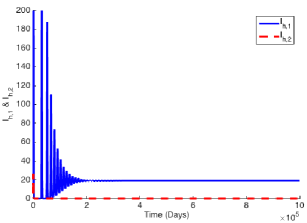
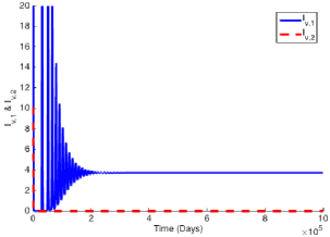
Figure 3: Dynamics of host and vectors if the host-vector configuration matrix is reducible.

5 Colima City and Manzanillo Dengue Inspired Simulation Study

Ae. aegypti was declared eradicated in Mexico in 1963. Not surprisingly, all four dengue serotypes (DENV-1, DENV-2, DENV-3 and DENV-4) re-emerged two years after local the 1963 eradication [23]. Further, DHF cases have steadily increased since 1994 [52]. Dengue is endemic in Mexico with approximately 60% of year-round cases reported in southern part of the country; a region is characterized by a warm and humid climate [21]. Colima, located on the central Pacific Coast (see Figure 4), is also a reservoir of Dengue. In 2002, the State of Colima reported 4,040 cases dengue in all of its 10 municipalities; 495 progressing to DHF [19, 25]. DENV-2 was isolated from patients during this outbreak [25]. The increase in DHF cases in Mexico has been linked to the introduction of DENV-2 Asian, previously isolated in 2000 and again in 2002 [43].

The dynamics of dengue are explored in the context of this 2002 State of Colima outbreak. The first reported (index) case was identified as that of a 10-year-old female in the municipality of Manzanillo on January 11, 2002. Dengue infection spread throughout the whole state with the most affected municipalities being Colima city, the capital of the state, and Manzanillo, an important tourist destination in the coast [25]. The city of Colima reported approximately 1,167 dengue cases, with 169 cases progressing to DHF while Manzanillo, reported 1,334 dengue cases, with 123 progressing to DHF in 2002 [18]. The city of Colima and Manzanillo are linked via high levels of travel and tourism. Both cities account for approximately 47% of the state population. We apply a two-patch model to explore the role that movement, modeled via the matrix $p_{ij}$, may have had on dengue disease transmission during this 2002 outbreak. The estimated population of Manzanillo and Colima City were $N_{h,1}=1,355$ and $N_{h,2}=1,184$, respectively, and the initial mosquito populations were choosen to best fit the data. They were approximately 308 and 738 in Manzanillo and Colima City, respectively. Note that the host population is not the actual population of the cities but rather the population at risk in each of the corresponding cities. The population at risk is much smaller that the actual population because in the same city there are social groups practically disconnected to others by geographic, cultural and social factors. Entomological parameters were estimated using [73] and taking into account the mean temperature in each region [18]. The remaining parameters used to study the outbreak in Colima, Mexico were obtained from the literature [1, 17, 29, 73]:

$$\beta_{hv}a_{1}=0.43\ \textrm{ days}^{-1},\ \beta_{hv}a_{2}=0.34\ \textrm{days}^{-1},\;\mu_{v}=0.036\ \textrm{(Colima)},\ 0.030\ \textrm{(Manzanillo)}\ \textrm{days}^{-1},\;$$

$$\frac{1}{\mu_{h}}=60\times 365\textrm{ days},\;\gamma_{1}=0.2\textrm{ days}^{-1},\;\gamma_{2}=0.2\textrm{ days}^{-1},\;\nu_{h}=0.18\textrm{ days}^{-1},\;\nu_{v}=0.1\textrm{ days}^{-1}.$$

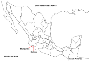
Figure 4: The state of Colima is located on the central Pacific coast of Mexico. It has a tropical climate, a surface of 5,455 $km^{2}$, and a population of approximately 488,028 inhabitants. The state of Colima is divided in 10 municipalities. Manzanillo, where the 2002 outbreak began, and Colima City are labeled in the map. $p_{11}=0.99$, $p_{22}=1.0$ with Manzanillo being represented with Patch 1 and Colima with Patch 2.

In order to assess, within our staged scenarios, the impact of migration during the 2002 dengue outbreak, we fit the two-patch model using the incidence data for Manzanillo and the city of Colima reported by the Mexican Social Security Institute (IMSS) during the outbreak (see Figure 5). The data fitting for cumulative dengue cases given by the model using ‘scipy.optimize.curve_fit’ library of python v2.7 programming language, is shown in Figure 7. Model results show that dengue spreads more quickly in the city of Colima when the proportion of visits from Manzanillo’s infected residents is high, see the left panel of Figure 6 compared with Figure 7. Alternatively, susceptible Colima City residents would acquire dengue infections over a longer time frame in Manzanillo, introducing the disease over a slower time scale in their home residence, the city of Colima. Of course, the absence of movement leads to no dengue cases in Manzanillo; an outbreak occurring only in Colima $p_{11}=p_{22}=1.0$, see center panel of Figure 6; equal movement, $p_{11}=p_{22}$, would cause the outbreak in Colima to grow faster, as can be seen in the right panel of Figure 6. Hence, limiting the movement of the Manzanillo population seems like a good strategy while limiting the movement of the Colima population wouldn’t be as effective. In the latest scenario, the economic cost would be high since Manzanillo is a tourist destination.

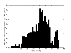
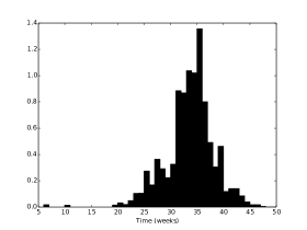
Figure 5: Incidence of dengue cases per weekly during the 2002 dengue epidemic diagnosed at the hospitals of the Mexican Institute of Public Health (IMSS) [18] in Manzanillo (left) and Colima city (right), respectively.

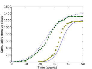
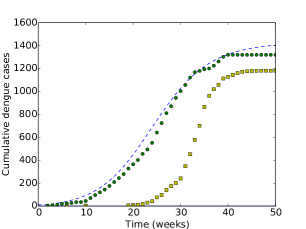
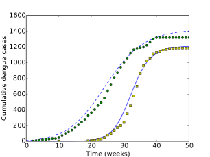
Figure 6: Circles: Cumulative dengue cases reported on Manzanillo, dotted line: Model prediction of Manzanillo cases, squares: Cumulative dengue cases reported on Colima city, solid line: Model prediction of cumulative cases in Colima city. Left: $p_{11}=1.0$, $p_{22}=0.9996$, Center: $p_{11}=1.0$, $p_{22}=1.0$, Right: $p_{11}=p_{22}=0.9996$ Patch 1 represents Manzanillo and patch 2 Colima.

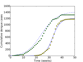
Figure 7: Best fit of the model $p_{11}=0.9996$, $p_{22}=1.0$. Circles: Cumulative dengue cases reported on Manzanillo, dotted line: Model prediction of Manzanillo cases, squares: Cumulative dengue cases reported on Colima city, solid line: Model prediction of cumulative cases in Colima city.

We can also observe in Figure 8 (on the left), that the effect of reducing the transit from Manzanillo to Colima city led only to a delay in the appearance of the outbreak in Colima. This indicates that the outbreak in Colima followed its own local dynamics and that transit between these two cities only led to delays in the introduction of the dengue virus without affecting the local outbreak dynamics. When the average visiting time spent in a place where the disease prevalence is low (small value of $p_{ij}$, $i\neq j$) then the only way of reducing an outbreak would require strict migration control, that is, complete travel avoidance to the high risk zone. In Figure 8 (on the right), we see that with only a small fraction of visitors from Manzanillo to Colima, the outbreaks in both cities occur almost simultaneously. Model simulations re-affirm the views that the rate of host movement and time spent in endemic geographic regions are important for the spread of dengue between two patches. The question then becomes, why aren’t then these residence times estimated?

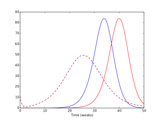
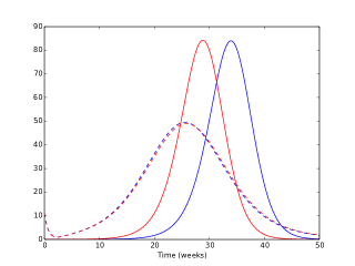
Figure 8: Dengue cases predicted by the model for Manzanillo (dotted line) and Colima city (solid line). In the first scenario (on the left), the blue lines represent no transit control and the red lines represent a reduction of 90% in movement from Manzanillo city to Colima. In the second scenario (on the right), the blue lines represent no movement control and the red lines represent an increment of movement from Colima to Manzanillo city of 1%.

6 Conclusion

The persistence of vector-bone diseases, such as dengue, is connected to factors that include the presence ecological conditions that favor high vector densities, vector-host interactions, the spatial movement of humans, and of course, the effectiveness of control measures [46, 69]. In this paper, a two-patch host-vector model was used to study the role of movement on the transmission dynamics of dengue, especially DENV-2. We focus on the applications of our framework to scenarios where dengue is endemic and where vertical transmission has been documented. A residence times matrix $\mathbb{P}$ is used to model host mobility. This modeling approach provides a framework for exploring spatial vector-borne disease dynamics and control within relatively “close’ environments. Analytical results were derived and the conditions for which the disease dies out or persists have been identified; conditions that depend on whether the basic reproduction number $\mathcal{R}_{0}(\mathbb{P})$ is less or greater than unity and the connectivity of patches.

Using data from the 2002 DENV-2 outbreak in Colima, Mexico, we compare the overall prevalence in the cities of Colima and Manzanillo as a function of pre-selected $\mathbb{P}$ matrices. Our model shows that reducing traveling from to Colima city, considered high-risk and the place of the 2002 outbreak onset, causes a slight delay in the spread of the disease. In order to completely prevent an outbreak in Colima city, migration between Colima city and Manzanillo must be stopped. Manzanillo a tourist destination implies that transit from Colima city to Manzanillo is expected to peak during certain seasons. The model suggests that dengue would become endemic in both patches almost simultaneously. The two-patch model highlights the role of human spatial movement on disease transmission and control. The strength of this effect depends on the proportion of time commuters to high or low risk spend in each patch.

Appendix A Appendix: The basic reproduction number

Let $x=(E_{h,1},E_{h,2},E_{v,1},E_{v,2},I_{h,1},I_{h,2},I_{v,1},I_{v,2})$ and so the relevant $\mathcal{F}$ and $\mathcal{V}$ are

$$\mathcal{F}=\left(\begin{array}[]{c}\frac{a_{1}\beta_{vh}p_{11}S_{h,1}I_{v,1}}{p_{11}N_{h,1}+p_{21}N_{h,2}}+\frac{a_{2}\beta_{vh}p_{12}S_{h,1}I_{v,2}}{p_{12}N_{h,1}+p_{22}N_{h,2}}\\ \frac{a_{1}\beta_{vh}p_{21}S_{h,2}I_{v,1}}{p_{11}N_{h,1}+p_{21}N_{h,2}}+\frac{a_{2}\beta_{vh}p_{22}S_{h,2}I_{v,2}}{p_{12}N_{h,1}+p_{22}N_{h,2}}\\ a_{1}\beta_{hv}S_{v,1}\frac{p_{11}I_{h,1}+p_{21}I_{h,2}}{p_{11}N_{h,1}+p_{21}N_{h,2}}\\ a_{2}\beta_{hv}S_{v,2}\frac{p_{12}I_{h,1}+p_{22}I_{h,2}}{p_{12}N_{h,1}+p_{22}N_{h,2}}\\ 0\\ 0\\ 0\\ 0\end{array}\right)\quad\text{and}\quad\mathcal{V}=\left(\begin{array}[]{c}-(\mu_{h}+\nu_{h})E_{h,1}\\ -(\mu_{h}+\nu_{h})E_{h,2}\\ -(\mu_{v}+\nu_{v})E_{v,1}\\ -(\mu_{v}+\nu_{v})E_{v,2}\\ \nu_{h}E_{h,1}-(\mu_{h}+\gamma_{i})I_{h,1}\\ \nu_{h}E_{h,2}-(\mu_{h}+\gamma_{i})I_{h,2}\\ \nu_{v}E_{h,1}-(1-q)\mu_{v}I_{v,1}\\ \nu_{v}E_{h,2}-(1-q)\mu_{v}I_{v,2}\end{array}\right).$$

Let $F\equiv D\mathcal{F}$ and $V\equiv D\mathcal{V}$ evaluated at the DFE. We obtain,

$$F=\left(\begin{array}[]{ccccc}0_{2,4}&\begin{array}[]{cc}0&0\\ 0&0\end{array}&\begin{array}[]{cc}\frac{a_{1}\beta_{vh}p_{11}N_{h,1}}{(1-p)\mu_{v}(p_{11}N_{h,1}+p_{21}N_{h,2})}&\frac{a_{2}\beta_{vh}p_{12}N_{h,1}}{(1-p)\mu_{v}(p_{12}N_{h,1}+p_{22}N_{h,2})}\\ \frac{a_{1}\beta_{vh}p_{21}N_{h,2}}{(1-p)\mu_{v}(p_{11}N_{h,1}+p_{21}N_{h,2})}&\frac{a_{2}\beta_{vh}p_{22}N_{h,2}}{(1-p)\mu_{v}(p_{12}N_{h,1}+p_{22}N_{h,2}}\end{array}\\ 0_{4,4}&\begin{array}[]{cc}\frac{a_{1}\beta_{vh}p_{11}N_{v,1}}{(\mu_{h}+\gamma_{1})(p_{11}N_{h,1}+p_{21}N_{h,2})}&\frac{a_{1}\beta_{vh}p_{21}N_{v,1}}{(\mu_{h}+\gamma_{2})(p_{11}N_{h,1}+p_{21}N_{h,2})}\\ \frac{a_{2}\beta_{vh}p_{12}N_{v,2}}{(\mu_{v})(p_{12}N_{h,1}+p_{22}N_{h,2})}&\frac{a_{2}\beta_{vh}p_{22}N_{v,2}}{(\mu_{h}+\gamma_{2})(p_{21}N_{h,1}+p_{22}N_{h,2}})\end{array}&0_{2,2}\\ 0_{4,4}&0_{4,2}&0_{4,2}\\ \end{array}\right)$$

and

$$V=\left(\begin{array}[]{cccccccc}-\mu_{h}-\nu_{h}&0&0&0&0&0&0&0\\ 0&-\mu_{h}-\nu_{h}&0&0&0&0&0&0\\ 0&0&-\mu_{v}-\nu_{v}&0&0&0&0&0\\ 0&0&0&-\mu_{v}-\nu_{v}&0&0&0&0\\ \nu_{v}&0&0&0&-\mu_{h}-\gamma_{1}&0&0&0\\ 0&\nu_{v}&0&0&0&\mu_{h}-\gamma_{h}&0&0\\ 0&0&\nu_{v}&0&0&0&-(1-p)\mu_{v}&0\\ 0&0&0&\nu_{v}&0&0&0&-(1-p)\mu_{v}\end{array}\right).$$

The basic reproduction number is the spectral radius of the matrix,

$$-FV^{-1}=\left(\begin{array}[]{cccccc}0_{2,2}&M_{vh}&\begin{array}[]{cc}0&0\\ 0&0\end{array}&\begin{array}[]{cc}\frac{a_{1}\beta_{vh}p_{11}N_{h,1}}{(1-q)\mu_{v}(p_{11}N_{h,1}+p_{21}N_{h,2})}&\frac{a_{2}\beta_{vh}p_{12}N_{h,1}}{(1-q)\mu_{v}(p_{12}N_{h,1}+p_{22}N_{h,2})}\\ \frac{a_{1}\beta_{vh}p_{21}N_{h,2}}{(1-q)\mu_{v}(p_{11}N_{h,1}+p_{21}N_{h,2})}&\frac{a_{2}\beta_{vh}p_{22}N_{h,2}}{(1-q)\mu_{v}(p_{12}N_{h,1}+p_{22}N_{h,2}}\end{array}\\ M_{hv}&0_{2,2}&\begin{array}[]{cc}\frac{a_{1}\beta_{vh}p_{11}N_{v,1}}{(\mu_{h}+\gamma_{1})(p_{11}N_{h,1}+p_{21}N_{h,2})}&\frac{a_{1}\beta_{vh}p_{21}N_{v,1}}{(\mu_{h}+\gamma_{2})(p_{11}N_{h,1}+p_{21}N_{h,2})}\\ \frac{a_{2}\beta_{vh}p_{12}N_{v,2}}{(\mu_{v})(p_{12}N_{h,1}+p_{22}N_{h,2})}&\frac{a_{2}\beta_{vh}p_{22}N_{v,2}}{(\mu_{h}+\gamma_{2})(p_{21}N_{h,1}+p_{22}N_{h,2}})\end{array}&0_{2,2}\\ 0_{4,2}&0_{4,2}&0_{4,2}&0_{4,2}\\ \end{array}\right)$$

where

$$M_{vh}=\left(\begin{array}[]{cc}\frac{a_{1}\beta_{vh}p_{11}N_{h,1}\nu_{v}}{(p_{11}N_{h,1}+p_{21}N_{h,2})(\mu_{v}+\nu_{v})(1-q)\mu_{v}}&\frac{a_{2}\beta_{vh}p_{12}N_{h,1}\nu_{v}}{(p_{12}N_{h,1}+p_{22}N_{h,2})(\mu_{v}+\nu_{v})(1-q)\mu_{v}}\\ \frac{a_{1}\beta_{vh}p_{21}N_{h,2}\nu_{v}}{(p_{11}N_{h,1}+p_{21}N_{h,2})(\mu_{v}+\nu_{v})(1-q)\mu_{v}}&\frac{a_{2}\beta_{vh}p_{22}N_{h,2}\nu_{v}}{(p_{12}N_{h,1}+p_{22}N_{h,2})(\mu_{v}+\nu_{v})(1-q)\mu_{v}}\end{array}\right)$$

and

$$M_{hv}=\left(\begin{array}[]{cc}\frac{a_{1}\beta_{hv}p_{11}N_{v,1}\nu_{h}}{(p_{11}N_{h,1}+p_{21}N_{h,2})(\mu_{h}+\nu_{h})(\mu_{h}+\gamma_{1})}&\frac{a_{1}\beta_{hv}p_{21}N_{v,1}\nu_{h}}{(p_{11}N_{h,1}+p_{21}N_{h,2})(\mu_{h}+\nu_{h})(\mu_{h}+\gamma_{2})}\\ \frac{a_{2}\beta_{hv}p_{12}N_{v,2}\nu_{h}}{(p_{12}N_{h,1}+p_{22}N_{h,2})(\mu_{h}+\nu_{h})(\mu_{h}+\gamma_{1})}&\frac{a_{2}\beta_{hv}p_{22}N_{v,2}\nu_{h}}{(p_{12}N_{h,1}+p_{22}N_{h,2})(\mu_{h}+\nu_{h})(\mu_{h}+\gamma_{2})}\end{array}\right).$$

The basic reproduction number $\mathcal{R}_{0}^{2}$ is defined by the expression,

$$\mathcal{R}_{0}^{2}=\rho(M_{vh}M_{hv}).$$

References

• [1] B. Adams and M. Boots, How important is vertical transmission in mosquitoes for the persistence of dengue? Insights from a mathematical model, Epidemics, 2 (2010), pp. 1–10.
• [2] B. Adams and D. D. Kapan, Man bites mosquito: understanding the contribution of human movement to vector-borne disease dynamics, (2009).
• [3] N. Arunachalam, S. Tewari, V. Thenmozhi, R. Rajendran, R. Paramasivan, R. Manavalan, K. Ayanar, and B. Tyagi, Natural vertical transmission of dengue viruses by Aedes aegypti in Chennai, Tamil Nadu, India, Indian J Med Res, 127 (2008), pp. 395–397.
• [4] P. Auger, E. Kouokam, G. Sallet, M. Tchuente, and B. Tsanou, The ross–macdonald model in a patchy environment, Mathematical biosciences, 216 (2008), pp. 123–131.
• [5] A. Balmaseda, S. Hammond, L. Perez, Y. Tellez, S. Saborio, J. Mercado, R. Cuadra, J. Rocha, M. Perez, S. Silva, et al., Serotype-specific differences in clinical manifestations of dengue, The American journal of tropical medicine and hygiene, 74 (2006), p. 449.
• [6] A. Berman and R. J. Plemmons, Nonnegative matrices, The Mathematical Sciences, Classics in Applied Mathematics, 9 (1979).
• [7] D. Bichara and C. Castillo-Chavez, Vector-borne diseases models with residence times-a lagrangian perspective, arXiv preprint arXiv:1509.08894, (2015).
• [8] D. Bichara, Y. Kang, C. Castillo-Chavez, R. Horan, and C. Perrings, Sis and sir epidemic models under virtual dispersal, Bulletin of mathematical biology, 77 (2015), pp. 2004–2034.
• [9] D. D. Bonnet and D. J. Worcester, The dispersal of aedes albopictus in the territory of hawaii, The American journal of tropical medicine and hygiene, 1 (1946), pp. 465–476.
• [10] C. Bosio, R. Thomas, P. Grimstad, and K. Rai, Variation in the efficiency of vertical transmission of dengue-1 virus by strains of Aedes albopictus (Diptera: Culicidae), Journal of medical entomology, 29 (1992), pp. 985–989.
• [11] F. Brauer and C. Castillo-Chávez, Mathematical models in population biology and epidemiology, vol. 40 of Texts in applied mathematics, Springer, 2012.
• [12] D. Burke, A. Nisalak, D. Johnson, and R. Scott, A prospective study of dengue infections in Bangkok, The American journal of tropical medicine and hygiene, 38 (1988), p. 172.
• [13] C. Castillo-Chávez, F. Sanchez, and D. Murillo, Change in host behavior and its impact on the transmission dynamics of dengue, BIOMAT Conference: International Symposium on Mathematical and Computational Biology, 9 (2011), pp. 1–13.
• [14] C. Castillo-Chavez and H. R. Thieme, Asymptotically autonomous epidemic models, in Mathematical Population Dynamics: Analysis of Heterogeneity, Volume One: Theory of Epidemics,, O. Arino, A. D.E., and M. Kimmel, eds., Wuerz, 1995.
• [15] CDC, Report Suggests Nearly 5 Percent Exposed to Dengue Virus in Key West, 2010.
• [16] A. Cecílio, E. Campanelli, K. Souza, L. Figueiredo, and M. Resende, Natural vertical transmission by Stegomyia albopicta as dengue vector in Brazil, Brazilian Journal of Biology, 69 (2009), pp. 123–127.
• [17] N. Chitnis, J. M. Hyman, and C. A. Manore, Modelling vertical transmission in vector-borne diseases with applications to rift valley fever, Journal of biological dynamics, 7 (2013), pp. 11–40.
• [18] G. Chowell, P. Diaz-Dueñas, J. Miller, A. Alcazar-Velazco, J. Hyman, P. Fenimore, and C. Castillo-Chavez, Estimation of the reproduction number of dengue fever from spatial epidemic data, Mathematical Biosciences, 208 (2007), pp. 571–589.
• [19] G. Chowell, P. Diaz-Duenas, D. Chowell, S. Hews, G. Ceja-Espiritu, J. M Hyman, and C. Castillo-Chavez, Clinical diagnosis delays and epidemiology of dengue fever during the 2002 outbreak in colima, mexico., (2007).
• [20] G. Chowell and F. Sanchez, Climate-based descriptive models of dengue fever: the 2002 epidemic in colima, mexico., Journal of environmental health, 68 (2006), pp. 40–4.
• [21] F. J. Colón-González, I. R. Lake, and G. Bentham, Climate variability and dengue fever in warm and humid mexico, The American journal of tropical medicine and hygiene, 84 (2011), pp. 757–763.
• [22] V. Deubel, R. M. Kinney, and D. W. Trent, Nucleotide sequence and deduced amino acid sequence of the nonstructural proteins of dengue type 2 virus, jamaica genotype: comparative analysis of the full-length genome, Virology, 165 (1988), pp. 234–244.
• [23] F. J. Díaz, W. C. Black, J. A. Farfán-Ale, M. A. Loroño-Pino, K. E. Olson, and B. J. Beaty, Dengue virus circulation and evolution in mexico: a phylogenetic perspective, Archives of medical research, 37 (2006), pp. 760–773.
• [24] O. Diekmann, J. A. P. Heesterbeek, and J. A. J. Metz, On the definition and the computation of the basic reproduction ratio $R_{0}$ in models for infectious diseases in heterogeneous populations, J. Math. Biol., 28 (1990), pp. 365–382.
• [25] F. Espinoza-Gómez, P. Díaz-Dueñas, C. Torres-Lepe, R. A. Cedillo-Nakay, and O. A. Newton-Sánchez, Clinical pattern of hospitalized patients during a dengue epidemic in colima, mexico, (2005).
• [26] L. Esteva and C. Vargas, Influence of vertical and mechanical transmission on the dynamics of dengue disease, Mathematical Biosciences, 167 (2000), pp. 51–64.
• [27] F. Forouzannia and A. B. Gumel, Mathematical analysis of an age-structured model for malaria transmission dynamics, Mathematical biosciences, 247 (2014), pp. 80–94.
• [28] D. Gao and S. Ruan, A multipatch malaria model with logistic growth populations, SIAM journal on applied mathematics, 72 (2012), pp. 819–841.
• [29] E. J. Garcí a Rivera and J. e. G. Rigau-P´erez, Dengue virus, in Congenital and Perinatal Infections, Springer, 2006, pp. 187–197.
• [30] A. Gumel, C. Castillo-Chavez, R. Mickens, and D. Clemence, Mathematical studies on human disease dynamics: emerging paradigms and challenges, American Mathematical Society, 2006.
• [31] J. Gunther, J. Martínez-Muñoz, D. Pérez-Ishiwara, and J. Salas-Benito, Evidence of vertical transmission of dengue virus in two endemic localities in the state of Oaxaca, Mexico, Intervirology, 50 (2007), pp. 347–352.
• [32] G. Guzman, G. Kouri, et al., Dengue and dengue hemorrhagic fever in the americas: lessons and challenges, Journal of Clinical Virology, 27 (2003), pp. 1–13.
• [33] S. Halstead, S. Nimmannitya, and S. Cohen, Observations related to pathogenesis of dengue hemorrhagic fever. IV. Relation of disease severity to antibody response and virus recovered., The Yale Journal of Biology and Medicine, 42 (1970), p. 311.
• [34] S. B. Halstead, N. T. Lan, T. T. Myint, T. N. Shwe, A. Nisalak, S. Kalyanarooj, S. Nimmannitya, S. Soegijanto, D. W. Vaughn, and T. P. Endy, Dengue hemorrhagic fever in infants: research opportunities ignored, Emerging infectious diseases, 8 (2002), pp. 1474–1479.
• [35] E. Harris, E. Videa, L. Perez, E. Sandoval, Y. Tellez, M. Perez, R. Cuadra, J. Rocha, W. Idiaquez, R. Alonso, et al., Clinical, epidemiologic, and virologic features of dengue in the 1998 epidemic in Nicaragua, The American journal of tropical medicine and hygiene, 63 (2000), p. 5.
• [36] W. Hawley, P. Reiter, R. Copeland, C. Pumpuni, and G. Craig Jr, Aedes albopictus in North America: probable introduction in used tires from northern Asia, Science, 236 (1987), p. 1114.
• [37] H. W. Hethcote and H. R. Thieme, Stability of the endemic equilibrium in epidemic models with subpopulations, Mathematical Biosciences, 75 (1985), pp. 205–227.
• [38] A. Iggidr, G. Sallet, and M. O. Souza, On the dynamics of a class of multi-group models for vector-borne diseases, arXiv preprint arXiv:1409.1470, (2014).
• [39] T. Knox, B. Kay, R. Hall, and P. Ryan, Enhanced vector competence of Aedes aegypti (Diptera: Culicidae) from the Torres Strait compared with mainland Australia for dengue 2 and 4 viruses, Journal of medical entomology, 40 (2003), pp. 950–956.
• [40] Y. Kwok, Dengue Fever Cases Reach Record Highs, in Time, 2010.
• [41] J. Kyle and E. Harris, Global spread and persistence of dengue, Annual Review of Microbiology, (2008).
• [42] J. Lewis, G. Chang, R. Lanciotti, R. Kinney, L. Mayer, and D. Trent, Phylogenetic relationships of dengue-2 viruses, Virology(New York, NY), 197 (1993), pp. 216–224.
• [43] M. A. Lorono-Pino, J. A. Farfan-Ale, A. L. Zapata-Peraza, E. P. Rosado-Paredes, L. F. Flores-Flores, J. E. Gardía-Rejón, F. J. Díaz, B. J. Blitvich, M. Andrade-Narvaez, E. Jimenez-Rios, et al., Introduction of the american/asian genotype of dengue 2 virus into the yucatan state of mexico, The American journal of tropical medicine and hygiene, 71 (2004), pp. 485–492.
• [44] A. Lotka, contribution to the analysis of malaria epidemiology, Am. J. Trop. Med. Hyg., 3 (1923), pp. 1–121.
• [45] G. Macdonald, The analysis of equilibrium in malaria., Tropical diseases bulletin, 49 (1952), pp. 813–829.
• [46] P. Martens and L. Hall, Malaria on the move: human population movement and malaria transmission., Emerging infectious diseases, 6 (2000), p. 103.
• [47] V. Martins, C. H. Alencar, M. T. Kamimura, F. M. de Carvalho Araujo, S. G. De Simone, R. F. Dutra, and M. Guedes, Occurrence of natural vertical transmission of dengue-2 and dengue-3 viruses in aedes aegypti and aedes albopictus in fortaleza, ceará, brazil, PloS one, 7 (2012), p. e41386.
• [48] F. McKenzie and E. Samba, The role of mathematical modeling in evidence-based malaria control, The American journal of tropical medicine and hygiene, 71 (2004), p. 94.
• [49] Y. Montoya, S. Holechek, O. Cáceres, A. Palacios, J. Burans, C. Guevara, F. Quintana, V. Herrera, E. Pozo, E. Anaya, et al., Circulation of dengue viruses in North-Western Peru, 2000-2001., Dengue Bulletin, 27 (2003).
• [50] D. Morens and A. Fauci, Dengue and hemorrhagic fever: A potential threat to public health in the United States, JAMA, 299 (2008), p. 214.
• [51] D. Murillo, S. A. Holechek, A. L. Murillo, F. Sanchez, and C. Castillo-Chavez, Vertical transmission in a two-strain model of dengue fever, Letters in Biomathematics, 1 (2014), pp. 249–271.
• [52] J. Navarrete-Espinosa, H. Gómez-Dantés, J. Germán Celis-Quintal, and J. L. Vázquez-Martínez, Clinical profile of dengue hemorrhagic fever cases in mexico, salud pública de méxico, 47 (2005), pp. 193–200.
• [53] G. A. Ngwa, A. M. Niger, and A. B. Gumel, Mathematical assessment of the role of non-linear birth and maturation delay in the population dynamics of the malaria vector, Applied Mathematics and Computation, 217 (2010), pp. 3286–3313.
• [54] M. Niebylski and G. Craig Jr, Dispersal and survival of aedes albopictus at a scrap tire yard in missouri., Journal of the American Mosquito Control Association, 10 (1994), pp. 339–343.
• [55] A. M. Niger and A. B. Gumel, Mathematical analysis of the role of repeated exposure on malaria transmission dynamics, Differential Equations and Dynamical Systems, 16 (2008), pp. 251–287.
• [56] H. Nishiura, Mathematical and statistical analyses of the spread of dengue, Dengue Bulletin, 30 (2006), p. 51.
• [57] S. of Hawaii, Dengue outbreak 2015. http://www.health.hawaii.gov/docd/dengue-outbreak-2015/. Accessed: December 30, 2015.
• [58] W. H. Organization, Dengue control. http://www.who.int/denguecontrol/mosquito/en/. Accessed: September 23, 2015.
• [59] Reiter, P. and Gubler, D.J., Surveillance and control of urban dengue vectors, Dengue and dengue hemorragic fever. New York: CAB International, (1997), pp. 45–60.
• [60] R. Rico-Hesse, L. Harrison, A. Nisalak, D. Vaughn, S. Kalayanarooj, S. Green, A. Rothman, and F. Ennis, Molecular evolution of dengue type 2 virus in Thailand, The American journal of tropical medicine and hygiene, 58 (1998), p. 96.
• [61] R. Rico-Hesse, L. Harrison, R. Salas, D. Tovar, A. Nisalak, C. Ramos, J. Boshell, M. de Mesa, R. Nogueira, and A. Rosa, Origins of dengue type 2 viruses associated with increased pathogenicity in the americas, Virology, 230 (1997), pp. 244–251.
• [62] F. Rodhain and L. Rosen, Mosquito vectors and dengue virus-vector relationships, Dengue and dengue hemorrhagic fever, (1997), pp. 112–134.
• [63] L. Rosen, D. Shroyer, R. Tesh, J. Freier, and J. Lien, Transovarial transmission of dengue viruses by mosquitoes: Aedes albopictus and Aedes aegypti, The American journal of tropical medicine and hygiene, 32 (1983), pp. 1108–1119.
• [64] R. Ross, The prevention of malaria, John Murray, 1911.
• [65] E. Shim, Z. Feng, and C. Castillo-Chavez, Differential impact of sickle cell trait on symptomatic and asymptomatic malaria, Mathematical biosciences and engineering: MBE, 9 (2012), p. 877.
• [66] N. Sittisombut, A. Sistayanarain, M. Cardosa, M. Salminen, S. Damrongdachakul, S. Kalayanarooj, S. Rojanasuphot, J. Supawadee, and N. Maneekarn, Possible occurrence of a genetic bottleneck in dengue serotype 2 viruses between the 1980 and 1987 epidemic seasons in Bangkok, Thailand, The American journal of tropical medicine and hygiene, 57 (1997), p. 100.
• [67] D. L. Smith, K. E. Battle, S. I. Hay, C. M. Barker, T. W. Scott, and F. E. McKenzie, Ross, macdonald, and a theory for the dynamics and control of mosquito-transmitted pathogens, PLoS pathog, 8 (2012), p. e1002588.
• [68] H. Smith and P. Waltman, The theory of the chemostat. Dynamics of microbial competition., Cambridge Studies in Mathematical Biology, Cambridge University Press, 1995.
• [69] R. W. Sutherst, Global change and human vulnerability to vector-borne diseases, Clinical microbiology reviews, 17 (2004), pp. 136–173.
• [70] S. Tewari, V. Thenmozhi, C. Katholi, R. Manavalan, A. Munirathinam, and A. Gajanana, Dengue vector prevalence and virus infection in a rural area in south India, Tropical Medicine and International Health, 9 (2004), pp. 499–507.
• [71] P. van den Driessche and J. Watmough, reproduction numbers and sub-threshold endemic equilibria for compartmental models of disease transmission, Math. Biosci., 180 (2002), pp. 29–48.
• [72] WHO, Dengue and dengue hemorrhagic fever. fact sheet, World Health Organization, (2009).
• [73] H. M. Yang, M. d. L. d. G. Macoris, K. C. Galvani, and M. T. M. Andrighetti, Follow up estimation of Aedes aegypti entomological parameters and mathematical modellings, Biosystems, 103 (2011), pp. 360–371.
• [74] C. Zhang, M. Mammen Jr, P. Chinnawirotpisan, C. Klungthong, P. Rodpradit, A. Nisalak, D. Vaughn, S. Nimmannitya, S. Kalayanarooj, and E. Holmes, Structure and age of genetic diversity of dengue virus type 2 in Thailand, Journal of General Virology, 87 (2006), p. 873.
• [75] X.-Q. Zhao, Dynamical systems in population biology, Springer Science & Business Media, 2013.