Covariate Balancing Propensity Score by Tailored Loss Functions

Abstract.

In observational studies, propensity scores are commonly estimated by maximum likelihood but may fail to balance high-dimensional pre-treatment covariates even after specification search. We introduce a general framework that unifies and generalizes several recent proposals to improve covariate balance when designing an observational study. Instead of the likelihood function, we propose to optimize special loss functions—covariate balancing scoring rules (CBSR)—to estimate the propensity score. A CBSR is uniquely determined by the link function in the GLM and the estimand (a weighted average treatment effect). We show CBSR does not lose asymptotic efficiency to the Bernoulli likelihood in estimating the weighted average treatment effect compared, but CBSR is much more robust in finite sample. Borrowing tools developed in statistical learning, we propose practical strategies to balance covariate functions in rich function classes. This is useful to estimate the maximum bias of the inverse probability weighting (IPW) estimators and construct honest confidence interval in finite sample. Lastly, we provide several numerical examples to demonstrate the trade-off of bias and variance in the IPW-type estimators and the trade-off in balancing different function classes of the covariates.

1. Introduction

To obtain causal relations from observational data, one crucial obstacle is that some pre-treatment covariates are not balanced between the treatment groups. Exact matching, inexact matching and subclassification on raw covariates were first used by pioneers like Cochran (1953, 1968) and Rubin (1973). Later in the seminal work of Rosenbaum and Rubin (1983), the propensity score, defined as the conditional probability of receiving treatment given the covariates, was established as a fundamental tool to adjust for imbalance in more than just a few covariates. Over the next three decades, numerous methods based on the propensity score have been proposed, most notably propensity score matching (e.g. Rosenbaum and Rubin, 1985, Abadie and Imbens, 2006), propensity score subclassification (e.g. Rosenbaum and Rubin, 1984), and inverse probability weighting (e.g. Robins et al., 1994, Hirano and Imbens, 2001); see Imbens (2004), Lunceford and Davidian (2004), Caliendo and Kopeinig (2008), Stuart (2010) for some comprehensive reviews.

With the rapidly increasing ability to collect high-dimensional covariates in the “big data” era (for example large number of covariates collected in health care claims data), propensity-score based methods often fail to produce satisfactory covariate balance (Imai et al., 2008). In the meantime, numerical examples in Smith and Todd (2005), Kang and Schafer (2007) have demonstrated that the average treatment effect estimates can be highly sensitive to the working propensity score model. Conventionally, these two issues are handled by a specification search—the estimated propensity score is applicable only if it balances covariates well. A simple strategy is to gradually increase the model complexity by forward stepwise regression (Imbens and Rubin, 2015, Section 13.3–13.4), but as a numerical example below indicates, this has no guarantee to achieve sufficient covariate balance eventually.

More recently, several new methods were proposed to directly improve covariate balance in the design of an observational study, either by modifying the propensity score model (Graham et al., 2012, Imai and Ratkovic, 2014) or by directly constructing sample weights for the observations (Hainmueller, 2011, Hazlett, 2016, Zubizarreta, 2015, Chan et al., 2016, Kallus, 2016). These methods have been shown to work very well empirically (particularly in finite sample) and some asymptotic justifications were subsequently provided (e.g. Zhao and Percival, 2016, Fan et al., 2016).

In this paper, we will introduce a general framework that unifies and generalizes these proposals. The solution provided here is conceptually simple: in order to improve covariate balance of a propensity score model, one just needs to minimize, instead of the most widely used negative Bernoulli likelihood, a special loss function tailored to the estimand.

1.1. A toy example

To demonstrate the simplicity and effectiveness of the tailored loss function approach, we use the prominent simulation example of Kang and Schafer (2007). In this example, for each unit $i=1,\dots,n=200$, suppose that $(Z_{i1},Z_{i2},Z_{i3},Z_{i4})^{T}$ is independently distributed as $\mathrm{N}(0,I_{4})$ and the true propensity scores are $p_{i}=P(T_{i}=1|Z_{i})=\mathrm{expit}(-Z_{i1}+0.5Z_{i2}-0.25Z_{i3}-0.1Z_{i4})$ where $T_{i}\in\{0,1\}$ is the treatment label. However, the observed covariates are nonlinear transformations of $Z$: $X_{i1}=\exp(Z_{i1}/2)$, $X_{i2}=Z_{i2}/(1+\exp(Z_{i1}))+10$, $X_{i3}=(Z_{i1}Z_{i3}/25+0.6)^{3}$, $X_{i4}=(Z_{i2}+Z_{i4}+20)^{2}$. To model the propensity score, we use a logistic model with some or all of $\{X_{1},X_{2},X_{3},X_{4},X_{1}^{2},X_{2}^{2},X_{3}^{2},X_{4}^{2}\}$ as regressors. Using forward stepwise regression, two series of models are fitted using the Bernoulli likelihood and the loss function tailored for estimating the average treatment effect (ATE, see Section 3.1 for more detail). Inverse probability weights (IPW) are obtained from each fitted model and standardized differences of the regressors are used to measure covariate imbalance (Rosenbaum and Rubin, 1985).

Figure 1 shows the paths of standardized difference for one realization of the simulation. A widely used criterion is that a standardized difference above 10% is unacceptable (Austin and Stuart, 2015, Normand et al., 2001), which is the dashed line in Figure 1. The left panel of Figure 1 uses the Bernoulli likelihood to fit and select logistic regression models. The standardized difference paths are not monotonically decreasing and never achieve the satisfactory level (10%) for all the regressors. In contrast, the right panel of Figure 1 uses the tailored loss function and all $8$ predictors are well balanced after $3$ steps. In fact, as a feature of using the tailored loss function, all active regressors (variables in the selected model) are exactly balanced.

The toy example here is merely for presentation, but it clearly demonstrates that the proposed tailored loss function approach excels in balancing covariates. We will discuss some practical strategies that are more sophisticated than the forward stepwise regression in Section 4.

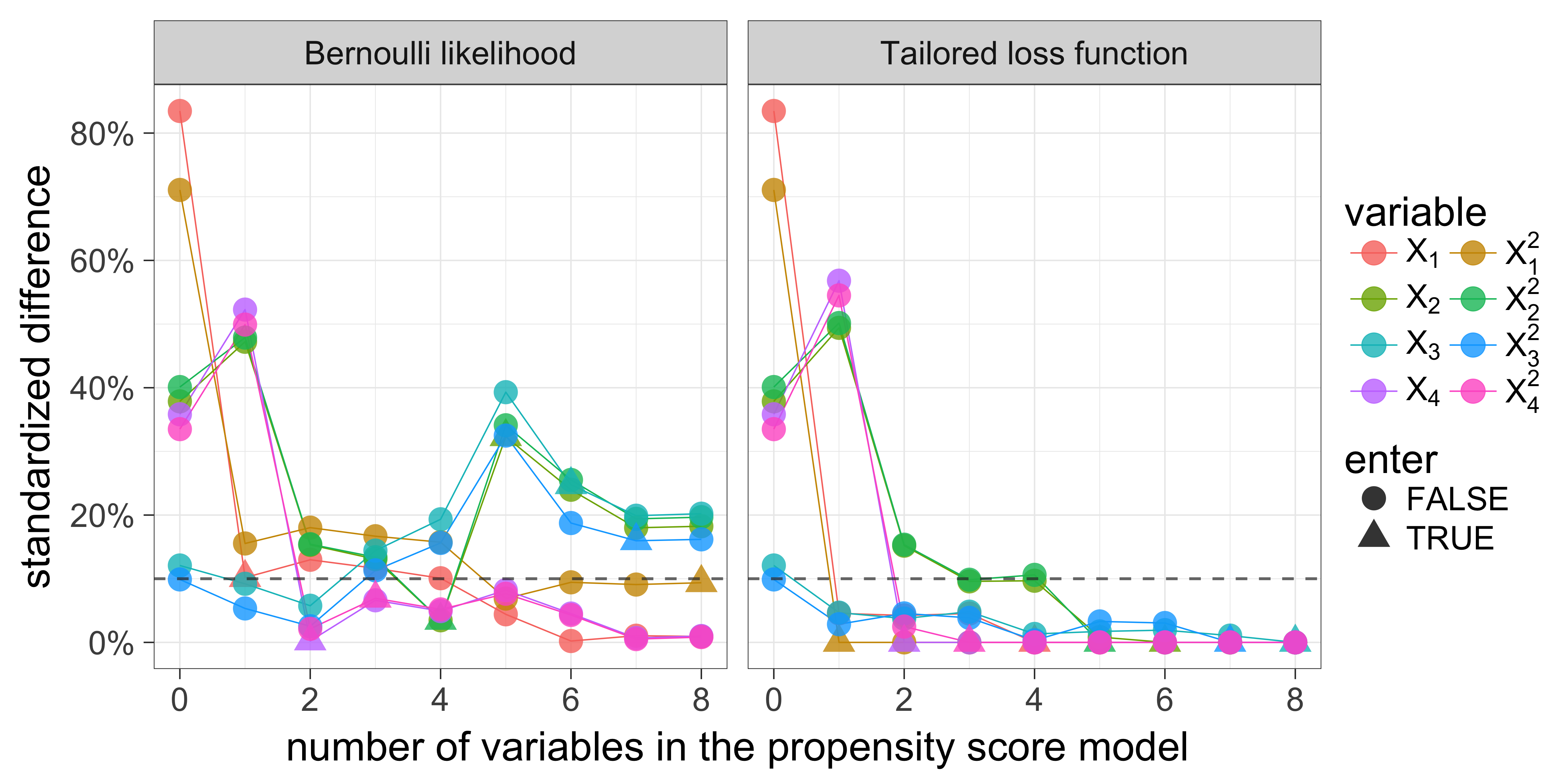
Figure 1. The tailored loss function proposed in this paper is much better than Bernoulli likelihood at reducing covariate imbalance. Propensity score is modeled by logistic regression and fitted by the tailored loss function or Bernoulli likelihood. Standardized difference is computed using inverse probability weighting (IPW) and pooled variance for the two treatment groups (Rosenbaum and Rubin, 1985). A standardized difference above 10% is often viewed unacceptable by many practitioners.

1.2. Related work and our contribution

The tailored loss function framework introduced here unifies a number of existing methods by exploring the (Lagrangian) duality of propensity scores and sample weights. Roughly speaking, the “moment condition” approaches advocated by Graham et al. (2012) and Imai and Ratkovic (2014) correspond to the primal problem of minimizing the tailored loss over propensity score models, while the “empirical balancing” proposals (e.g. Hainmueller, 2011, Zubizarreta, 2015) correspond to the dual problem that solves some convex optimization problem over the sample weights subject to covariate balance constraints. The framework presented here is largely motivated by the aforementioned works. Part of the contribution of this paper is to bring together many pieces scattered in this literature—moment condition of estimating the propensity score, covariate balance, bias-variance trade-off, different estimands, link function of a generalized linear model (the latter two are often overlooked)—and elucidate their roles in the design and analysis of an observational study.

A reader familiar with the development of this literature may recognize that many elements in the framework proposed here have already appeared in some previous works. Perhaps the closest approach is the covariate balancing propensity score method of Imai and Ratkovic (2014), as their covariate balancing moment conditions are essentially the first-order conditions of minimizing the tailored loss function. In fact, this is the reason that “covariate balancing propensity score” is kept in the title of this paper. However, by taking a loss-function based approach, we can

• Visualize the tailored loss functions which penalize more heavily on larger inverse probability weights and hence generates more stable estimates. (See the supplementary file for more detail.)

• Understand when the moment equations have a unique solution by investigating convexity of the loss function. This may limit the estimands and link functions one can use in practice, though it turns out that for the logistic link function most of the commonly used estimands correspond to convex problems.

• More importantly, allow the usage of predictive algorithms developed in statistical learning to optimize covariate balance in high-dimensional problems and rich function classes. Moment constraints methods usually exactly balance several selected covariate functions but leave the others unattended. By regularizing the tailored loss function, a signature technique in predictive modeling, the methods proposed in Section 4 can inexactly balance high-dimensional or even infinite-dimensional covariate functions. This usually results in more accurate estimates of the weighted average treatment effects (WATE) and more robust statistical inference.

Compared to the empirical balancing methods, the tailored loss function framework shows that they are essentially equivalent to certain models of propensity score. Asymptotic theory that are already established to propensity-score based estimators can now apply to empirical balancing methods. Our framework also allows the use of balancing weights in estimating more general estimands. For example, we can produce balancing weights to estimate the optimally weighted average treatment effect proposed by Crump et al. (2006) that is more stable when there is limited overlap (Li et al., 2016).

Last but not the least, we provide a novel approach to make honest, design-based and finite-sample inference for the weighted average treatment effects (WATE). Instead of the improbable but commonly required assumption that the propensity score is correctly specified, the only major assumption we make is that the (unkonwn) true outcome regression function is in a given class. The function class can be high-dimensional and very rich. We give a Bayesian interpretation that underlies any design of an observational study and provide extensive numerical results to demonstrate the trade-off in making different assumptions about the outcome regression function.

The next two Sections are devoted to introducing the tailored loss functions. Section 4 propose practical strategies motivated by statistical learning. Section 5 then considers some theoretical aspects about the tailored loss functions. Section 6 uses numerical examples in two new settings to demonstrate the flexibility of the proposed framework and examine its empirical performance. Section 7 concludes the paper with some practical recommendations. Technical proofs are provided in the supplementary file.

2. Preliminaries on Statistical Decision Theory

To start with, propensity score estimation can be viewed as a decision problem and this Section introduce some terminologies in statistical decision theory. In a typical problem of making probabilistic forecast, the decision maker needs to pick an element as the prediction from $\mathcal{P}$, a convex class of probability measures on some general sample space ${\Omega}$. For example, a weather forecaster needs to report the chance of rain tomorrow, so the sample space is $\Omega=\{\mathrm{rain},\mathrm{no~{}rain}\}$ and the prediction is a Bernoulli distribution. Propensity score is a (conditional) probability measure, but recall that the goal is to achieve satisfactory covariate balance rather than the best prediction of treatment assignment. At a high level, this is precisely the reason why we want to tailor the loss function when estimating the propensity score.

2.1. Proper scoring rules

At the core of statistical decision theory is the scoring rule, which can be any extended real-valued function $S:\mathcal{P}\times\Omega\to[-\infty,\infty]$ such that $S(P,\cdot)$ is $\mathcal{P}$-integrable for all $P\in\mathcal{P}$ (Gneiting and Raftery, 2007). If the decision is $P$ and $\omega$ materializes, the decision maker’s reward or utility is $S(P,\omega)$. An equivalent but more pessimistic terminology is loss function, which is just the negative scoring rule. These two terms will be used interchangeably in this paper.

If the outcome is probabilistic in nature and the actual probability distribution is $Q$, the expected score of forecasting $P$ is

$$S(P,Q)=\int S(P,\omega)Q(d\omega).$$

To encourage honest decisions, the scoring rule $S$ is generally required to be proper,

$$S(Q,Q)\geq S(P,Q),\quad\forall P,Q\in\mathcal{P}.$$ (1)

The rule is called strictly proper if (1) holds with equality if and only if $P=Q$.

In observational studies, the sample space is commonly dichotomous $\Omega=\{0,1\}$ (two treatment groups: $0$ for control and $1$ for treated), though there is no essential difficulty to extend the approach in this paper to $|\Omega|>2$ (multiple treatments) or $\Omega\subset\mathbb{R}$ (continuous treatment). In the binary case, a probability distribution $P$ can be characterized by a single parameter $0\leq p\leq 1$, the probability of treatment. A classical result of Savage (1971) asserts that every real-valued (except for possibly $S(0,1)=\infty$ or $S(1,0)=-\infty$) proper scoring rule $S$ can be written as

$$\begin{split}S(p,1)&=G(p)+(1-p)G^{\prime}(p)=\int(1-p)G^{\prime\prime}(p)dp+\mathrm{const},\\ S(p,0)&=G(p)-pG^{\prime}(p)=-\int pG^{\prime\prime}(p)dp+\mathrm{const},\\ \end{split}$$

where $G:[0,1]\to\mathbb{R}$ is a convex function and $G^{\prime}(p)$ is a subgradient of $G$ at the point $p\in[0,1]$. When $G$ is second-order differentiable, an equivalent but more convenient representation is

$$\frac{\partial}{\partial p}S(p,t)=(t-p)G^{\prime\prime}(p),~{}t=0,1.$$ (2)

Since the function $G$ uniquely defines a scoring rule $S$, we shall call $G$ a scoring rule as well.

A useful class of proper scoring rules is the following Beta family

$$G_{\alpha,\beta}^{\prime\prime}(p)=p^{\alpha-1}(1-p)^{\beta-1},~{}-\infty<\alpha,\beta<\infty.$$ (3)

These scoring rules were first introduced by Buja et al. (2005) to approximate the weighted misclassification loss by taking the limit $\alpha,\beta\to\infty$ and $\alpha/\beta\to c$. For example, if $c=1$, the score $G_{\alpha,\beta}$ converges to the zero-one misclassification loss. Many important scoring rules belong to this family. For example, the Bernoulli log-likelihood function $S(p,t)=t\log p+(1-t)\log(1-p)$ corresponds to $\alpha=\beta=0$, and the Brier score or the squared error loss $S(p,t)=-(t-p)^{2}$ corresponds to $\alpha=\beta=1$. For our purpose of estimating propensity score, it will be shown later that the subfamily $-1\leq\alpha,\beta\leq 0$ is particularly useful.

2.2. Propensity score modeling by maximizing score

Given i.i.d. observations $(X_{i},T_{i})\in\mathbb{R}^{d}\times\{0,1\},~{}i=1,2,\dotsc,n$ where $T_{i}$ is the binary treatment assignment and $X_{i}$ is a vector of $d$ pre-treatment covariates, we want to fit a model for the propensity score $p(X)=\mathrm{P}(T=1|X)$ in a prespecified family $\mathcal{P}=\{p_{\theta}(X):\theta\in\Theta\}$. Later on we will consider very rich model family, but for now let’s focus on the generalized linear models with finite-dimensional regressors $\phi(X)=(\phi_{1}(X),\dotsc,\phi_{m}(X))^{T}$ (McCullagh and Nelder, 1989)

$$p_{\theta}(X)=l^{-1}(f_{\theta}(X))=l^{-1}(\theta^{T}\phi(X)),$$ (4)

where $l$ is the link function. In our framework, the tailored loss function is determined by the link function $l$ (and the estimand). The most common choice is the logistic link

$$l(p)=\log\frac{p}{1-p},~{}l^{-1}(f)=\frac{e^{f}}{1+e^{f}},$$ (5)

which will be used in all the numerical examples of this paper.

Given a strictly proper scoring rule $S$, the maximum score (minimum loss) estimator of $\theta$ is obtained by maximizing the average score

$$\hat{\theta}_{n}=\arg\max_{\theta}\mathcal{S}_{n}(\theta)=\frac{1}{n}\sum_{i=1}^{n}S(p_{\theta}(X_{i}),T_{i}).$$ (6)

Notice that an affine transformation $S(p,t)\mapsto aS(p,t)+b(t)$ for any $a>0$ and $-\infty<b(t)<\infty$ gives the same estimator $\hat{\theta}_{n}$. Due to this reason, we will not differentiate between these equivalent scoring rules and use a single function $S(p,t)$ to represent all the equivalent ones.

When $S$ is differentiable and assuming exchangeability of taking expectation and derivative, the maximizer of $\mathrm{E}[\mathcal{S}_{n}(\theta)]$, which is indeed $\theta$ if the propensity score is correctly specified $p(x)=p_{\theta}(x)$ (a property called Fisher-consistency), is characterized by the following estimating equations

$$\nabla_{\theta}\,\mathrm{E}[\mathcal{S}_{n}(\theta)]=\mathrm{E}[\nabla_{\theta}\,\mathcal{S}_{n}(\theta)]=\mathrm{E}_{X,T}[\nabla_{\theta}\,S(l^{-1}(\theta^{T}\phi(X)),T)]=0.$$ (7)

3. Tailoring the loss function

3.1. Covariate balancing scoring rules

The tailored loss function framework is motivated by reinterpreting the first-order conditions (7) as covariate balancing constraints. Using the representation (2) and the inverse function theorem, we can rewrite (7) as

$$\mathrm{E}[(T-(1-T))w(X,T)\cdot\phi(X)]=0,$$ (8)

where the weighting function

$$w(x,t)=\frac{G^{\prime\prime}(p(x))}{l^{\prime}(p(x))}[t(1-p(x))+(1-t)p(x)]$$ (9)

is determined by the scoring rule through $G^{\prime\prime}$ and the link function $l$. The maximum score estimator $\hat{\theta}_{n}$ can be obtained by solving (8) with the expectation over the empirical distribution of $(X,T)$ instead of the population. When the optimization problem (6) is strongly convex, the solution to (8) is also unique.

The next key observation is that every weighting function $w(x,t)$ defines a weighted average treatment effect (WATE). To see this, we need to introduce the Neyman-Rubin causal model. Let $Y(t),~{}t=0,1$ be the potential outcomes and $Y=TY(1)+(1-T)Y(0)$ be the observed outcome. This paper assumes strong ignorability of treatment assignment (Rosenbaum and Rubin, 1983), so the observational study is free of hidden bias:

Assumption 1.

$T\mathchoice{\mathrel{\hbox to0.0pt{$\displaystyle\perp$\hss}\mkern 2.0mu{\displaystyle\perp}}}{\mathrel{\hbox to0.0pt{$\textstyle\perp$\hss}\mkern 2.0mu{\textstyle\perp}}}{\mathrel{\hbox to0.0pt{$\scriptstyle\perp$\hss}\mkern 2.0mu{\scriptstyle\perp}}}{\mathrel{\hbox to0.0pt{$\scriptscriptstyle\perp$\hss}\mkern 2.0mu{\scriptscriptstyle\perp}}}(Y(0),Y(1))|X$.

Let the observed outcomes be $Y_{i}$, $i=1,\dotsc,n$. Naturally, the weighted difference of $Y_{i}$,

$$\hat{\tau}=\sum_{i:\,T_{i}=1}w(X_{i},T_{i})Y_{i}-\sum_{i:\,T_{i}=0}w(X_{i},T_{i})Y_{i},$$ (10)

estimates the following population parameter

$$\tau_{v}=\mathrm{E}_{X,T,Y}\{(T-(1-T))w(X,T)Y\}=\mathrm{E}_{X,Y}\left[v(X)(Y(1)-Y(0))\right],$$

which is an (unnormalized) weighted average treatment effect. Here

$$v(X)=\mathrm{E}[T\cdot w(X,1)|X]=\mathrm{E}[(1-T)\cdot w(X,0)|X]=\frac{G^{\prime\prime}(p(X))\,p(X)\,(1-p(X))}{l^{\prime}(p(X))}.$$ (11)

In practice, it is usually more meaningful to estimate the normalized version $\tau_{w}^{*}=\tau_{w}/\mathrm{E}\left[w(X)\right]$ by normalizing the weights $w_{i}=w(X_{i},T_{i}),~{}i=1,\dotsc,n$ separately among the treated and the control: $\hat{w}_{i}^{*}=\hat{w}_{i}/\sum_{j:\,T_{j}=T_{i}}\hat{w}_{j}$, $i=1,\dotsc,n$.

Table 1 shows that four mostly commonly used estimands, the average treatment effect (ATE), the average treatment effect on the control (ATC), the average treatment effect on the treated (ATT), and the optimally weighted average treatment effect (OWATE) under homoscedasticity (Crump et al., 2006), are weighted average treatment effects with

$$v_{\alpha,\beta}(X)=p({X})^{\alpha+1}(1-p({X}))^{\beta+1}$$ (12)

with different combinations of $(\alpha,\beta)$.

Table 1. Correspondence of estimands, sample weighting functions, and the covariate balancing scoring rules (corresponding to the logistic link) in the proposed Beta family. The estimand is a weighted average treatment effect $\tau_{\alpha,\beta}=\mathrm{E}\left[v_{\alpha,\beta}(X)(Y(1)-Y(0))\right]$ and $\tau^{*}=\tau_{\alpha,\beta}/\mathrm{E}[v_{\alpha,\beta}(X)]$.

$\alpha$	$\beta$	estimand	$w(x,1)$	$w(x,0)$	$S(p,1)$	$S(p,0)$
-1	-1	$\tau=\tau^{*}=\mathrm{E}[Y(1)-Y(0)]$	$\frac{1}{p(x)}$	$\frac{1}{1-p(x)}$	$\log\frac{p}{1-p}-\frac{1}{p}$	$\log\frac{1-p}{p}-\frac{1}{1-p}$
-1	0	$\tau^{*}=\mathrm{E}[Y(1)-Y(0)|T=0]$	$\frac{1-p(x)}{p(x)}$	$1$	$-\frac{1}{p}$	$\log\frac{1-p}{p}$
0	-1	$\tau^{*}=\mathrm{E}[Y(1)-Y(0)|T=1]$	$1$	$\frac{p(x)}{1-p(x)}$	$\log\frac{p}{1-p}$	$-\frac{1}{1-p}$
0	0	$\tau=\mathrm{E}[p(X)(1-p(X))\cdot(Y(1)-Y(0))]$	$1-p(x)$	$p(x)$	$\log p$	$\log(1-p)$

Therefore, in order to estimate $\tau_{\alpha,\beta}=\mathrm{E}[v_{\alpha,\beta}(X)(Y(1)-Y(0))]$, we just need to equate (11) with (12) and solve for $G$. The solution in general depends on the link function $l$. If the logistic link is used, it is easy to show that the solution belongs to the Beta family of scoring rules defined in (3). The loss functions corresponding to the four estimands are also listed in (12).

Proposition 1.

Under Assumption 1, if $l$ is the logistic link function, then $\tau_{v}=\tau_{\alpha,\beta}$ if $G=G_{\alpha,\beta}$.

To use the framework developed here in practice, the user should “invert” the development in this Section. First, the user should determine the estimand by its interpretation and whether there is insufficient covariate overlap (so OWATE may be desirable). Second, the user should decide on a link function (we recommend logistic link). Lastly, the user can equate (11) with (12) or look up Table 1 to find the corresponding scoring rule.

The main advantage of using the “correct” scoring rule is that the weights will automatically balance the predictors $\phi(X)$. This is a direct consequence of the estimating equations (8) and is summarized in the next theorem. This is precisely the reason we call $G_{\alpha,\beta}$ or the corresponding $S_{\alpha,\beta}$ the covariate balancing scoring rule (CBSR) with respect to the estimand $\tau_{\alpha,\beta}$ and the logistic link function in this paper.

Theorem 1.

If $l$ is the logistic link function and $\hat{\theta}$ is obtained as in (6) by maximizing the CBSR corresponding to $l$ and the estimand. Then the weights $\hat{w}_{i},~{}i=1,\dotsc,n$ computed by (9) exactly balance the sample regressors

$$\sum_{i:\,T_{i}=1}\hat{w}_{i}\phi(X_{i})=\sum_{i:\,T_{i}=0}\hat{w}_{i}\phi(X_{i}).$$ (13)

Furthermore, if the predictors include an intercept term (i.e. $1$ is in the linear span of $\phi(X)$), then $\hat{w}^{*}$ also satisfies (13).

Note that the Bernoulli likelihood ($\alpha=\beta=0$) indeed corresponds to the estimand OWATE instead of the more commonly used ATE or ATT. This corresponds to the “overlap weights” recently proposed by Li et al. (2016), where each observation’s weight is proportional to the probability of being assigned to the opposite group. Theorem 3 of Li et al. (2016) states that the “overlap weights” exactly balances the regressors when Bernoulli likelihood is used, which is a special case of our Theorem 1.

3.2. Convexity

To obtain covariate balancing propensity scores, one can solve the estimating equations (8) directly without using the tailored loss function. This is essentially the approach taken by Imai and Ratkovic (2014), although it is unclear at this point that (13) has a unique solution. The first advantage of introducing the tailored loss functions is that some CBSR is strongly concave, so the solution to its first-order condition is always unique.

Proposition 2.

Suppose the estimand is in the Beta-family Equation 12 and let $S$ be the CBSR corresponding to a link function $l$ such that $v=v_{\alpha,\beta}$. Then the score functions $S(l^{-1}(f),0)$ and $S(l^{-1}(f),1)$ are both concave functions of $f\in\mathbb{R}$ if and only if $-1\leq\alpha,\beta\leq 1$. Moreover, if $(\alpha,\beta)\neq(-1,0)$, $S(l^{-1}(f),0)$ is strongly concave; if $(\alpha,\beta)\neq(0,-1)$, $S(l^{-1}(f),1)$ is strongly concave.

Notice that the range of $(\alpha,\beta)$ in Proposition 2 includes the four estimands listed in Table 1. As a consequence, their corresponding score maximization problems can be solved very efficiently (for example by Newton’s method). Motivated by this observation, in the next Section we propose to fit propensity score models with more sophisiticated strategies stemming from statistical learning.

4. Adaptive Strategies

The generalized linear model considered in Section 3 amounts to a fixed low-dimensional model space

$$\mathcal{P}_{\mathrm{GLM}}=\Big{\{}p(x)=l^{-1}(f(x)):\,f(x)\in\mathrm{span}(\phi_{1}(x),\phi_{2}(x),\dotsc,\phi_{m}(x))^{T}\Big{\}}.$$

As mentioned previously in Section 1, in principle, we should not restrict to a single propensity score model as it can be misspecified. Propensity score is merely a nuisance parameter in estimating WATE. We shall see repeatedly in later Sections that, in finite sample, it is more important to use flexible propensity score models that balance covariates well than to estimate the propensity score accurately. In this Section, we incorporate machine learning methods in our framework to expand the model space.

4.1. Forward stepwise regression

To increase model complexity, perhaps the most straightforward approach is forward stepwise regression as illustrated earlier in Section 1. Instead of a fixed model space, forward stepwise gradually increases model complexity. Using the tailored loss functions in Section 3, active covariates are always exactly balanced and inactive covariates are usually well balanced too.

Motivated by this strategy, Hirano, Imbens, and Ridder (2003) studied the efficiency of the IPW estimator when the dimension of the regressors $\phi(x)$ is allowed to increase as the sample size $n$ grows. Their renowned results claim that this sieve IPW estimator is semiparametrically efficient for estimating the WATE. Here we show that the semiparametric efficiency still holds if the Bernoulli likelihood, the loss function that Hirano et al. (2003) used to estimate the propensity score, is replaced by the Beta family of scoring rules $G_{\alpha,\beta}$, $-1\leq\alpha,\beta\leq 0$ in (3) or essentially any strongly concave scoring rule. This result is not too surprising as the propensity score is just a nuisance parameter whose estimation accuracy is of less importance in semiparametric inference. Conceptually, however, this result suggests that the investigator has the freedom to choose the loss function in estimating the propensity score and do not need to worry about loss of asymptotic efficiency. The advantages of using a tailored loss function are better accuracy in finite sample and more robustness against model misspecification, as detailed later in the Section 5.

Let’s briefly review the sieve logistic regression in Hirano et al. (2003). For $m=1,2,\dotsc$, let ${\phi}_{m}({x})=(\varphi_{1m}({x}),\varphi_{2m}({x}),\dotsc,\varphi_{mm}({x}))^{T}$ be a triangular array of orthogonal polynomials, which are obtained by orthogonalizing the power series: $\psi_{km}({x})=\prod_{j=1}^{d}x_{j}^{\gamma_{kj}}$, where ${\gamma}_{k}=(\gamma_{k1},\dotsc,\gamma_{kd})^{T}$ is an $d$-dimensional multi-index of nonnegative integers and satisfies $\sum_{j=1}^{d}\gamma_{kj}\leq\sum_{j=1}^{d}\gamma_{k+1,j}$. Let $l$ be the logistic link function (5). Hirano et al. (2003) estimated the propensity score by maximizing the log-likelihood

$$\hat{{\theta}}^{\mathrm{MLE}}=\arg\max_{{\theta}}\frac{1}{n}\sum_{i=1}^{n}T_{i}\log\left(l^{-1}({\phi}_{m}({X}_{i})^{T}{\theta})\right)+(1-T_{i})\log\left(1-l^{-1}({\phi}_{m}({X}_{i})^{T}{\theta})\right).$$

This is a special case of the score maximization problem (6) by setting $S=S_{0,0}$.

Theorem 2 below is an extension to the main theorem of Hirano et al. (2003). Besides strong ignorability, the other technical assumptions in Hirano et al. (2003) are listed in the supplement. Compared to the original theorem which always uses the maximum likelihood regardless of the estimand, the scoring rule is now tailored according to the estimand as described in Section 3.

Theorem 2.

Suppose we use the Beta-family of covariate balancing scoring rules defined by equations 2 and 3 with $-1\leq\alpha,\beta\leq 0$ and the logistic link (5). Under Assumption 1 and the technical assumptions in Hirano et al. (2003), if we choose suitable $m$ growing with $n$, the propensity score weighting estimator $\hat{\tau}_{\alpha,\beta}$ and its normalized version $\hat{\tau}_{\alpha,\beta}^{*}$ are consistent for $\tau_{\alpha,\beta}$ and $\tau_{\alpha,\beta}^{*}$. Moreover, they reach the semiparametric efficiency bound for estimating $\tau_{\alpha,\beta}$ and $\tau_{\alpha,\beta}^{*}$.

4.2. Regularized Regression

In predictive modeling, stepwise regression is usually sub-optimal especially if we have high dimensional covariates (see e.g. Hastie et al., 2009, Section 3). A more principled approach is to penalize the loss function

$$\hat{\theta}_{\lambda}=\arg\max_{p(\cdot)\in\mathcal{P}}~{}\frac{1}{n}\sum_{i=1}^{n}S(p({X}_{i}),T_{i})-\lambda J(p(\cdot)),~{}p(x)=l^{-1}(f(x)),$$ (14)

where $J(\cdot)$ is a regularization function that penalizes overly-complicated propensity score model $p(x)$ and the tuning parameter $\lambda$ controls the degree of regularization. This estimator reduces to the optimum score estimator (6) when $\lambda=0$.

The penalty term $J(\theta)$ should be chosen according to the model space $\mathcal{P}$ and the investigator’s prior belief about the outcome regression function (see Section 5.4). In this paper, we consider three alternatives of model space and penalty:

1. Regularized GLM: the model space is the same generalized linear model $\mathcal{P}_{\mathrm{GLM}}$ with potentially high dimensional covariates, but the average score is penality by the $l_{a}$-norm of $\theta$, $J(p_{\theta})=\frac{1}{a}\sum_{k=1}^{m}|\theta_{k}|^{a}$ for some $a\geq 1$. Some typical choices are the $l_{1}$ norm $J(p_{\theta})=\|{\theta}\|_{1}$ (lasso) and the squared $l_{2}$ norm $J(p_{\theta})=\|{\theta}\|_{2}^{2}$ (ridge regression).

2. Reproducing kernel Hilbert space (RKHS): the model space is the RKHS generated by a given kernel $K$, $\mathcal{P}_{\mathrm{RKHS}}=l^{-1}(\mathcal{H}_{K})$, and the penalty is the corresponding norm of $f$, $J(p(\cdot))=\|f\|_{\mathcal{H}_{K}}$.

3. Boosted trees: the model space is the additive trees: $\mathcal{P}_{k\textrm{-}\mathrm{boost}}=\{p(x)=l^{-1}(f(x)):f=f_{1}+f_{2}+\cdots+f_{m}:f_{k}\in\mathcal{F}_{\mathrm{d\textrm{-tree}}},~{}k=1,2,\dotsc\}$, where $\mathcal{F}_{\mathrm{d\textrm{-tree}}}$ is the space of step functions in the classification and regression tree (CART) with depth at most $d$ (Breiman et al., 1984). This space is quite large and approximate fitting algorithms (boosting) must be used. There is no exact penalty function, but as noticed by Friedman et al. (1998) and illustrated later, boosting is closely related to the lasso penalty in regularized regression.

Since all the penalty terms considered here are conex, the regularized optimization problems can be solved very efficiently.

4.3. RKHS regression

Next, we elaborate on the RKHS and boosting approaches since they might be foreign to researchers in causal inference. RKHS regression is a popular nonparametric method in machine learning that essentially extends the regularized GLM with ridge penalty to an infinite dimensional space (Wahba, 1990, Hofmann et al., 2008). Let $\mathcal{H}_{K}$ be the RKHS generated by the kernel function $K:\mathcal{X}\times\mathcal{X}\to\mathbb{R}$, which describes similarity between two vectors of pre-treatment covariates. The RKHS model is most easily understood through the “feature map” interpretation. Suppose that $K$ has an eigen-expansion $K({x},{x}^{\prime})=\sum_{k=1}^{\infty}c_{k}\phi_{k}({x})\phi_{k}({x}^{\prime})$ with $c_{k}\geq 0,~{}\sum_{k=1}^{\infty}c_{k}^{2}<\infty$. Elements of $\mathcal{H}_{K}$ have a series expansion

$$f({x})=\sum_{k=1}^{\infty}\theta_{k}\phi_{k}({x}),~{}\|f\|_{\mathcal{H}_{K}}^{2}=\sum_{k=1}^{\infty}\theta_{k}^{2}/c_{k}.$$

The eigen-functions $\{\phi_{1}(x),\phi_{2}(x),\dotsc,\}$ can be viewed as new regressors generated by the low-dimensional covariates $X$. The standard generalized linear model (4) corresponds to a finite-dimensional linear reproducing kernel $K({x},{x}^{\prime})=\sum_{k=1}^{m}\phi_{k}({x})\phi_{k}({x}^{\prime})$, but in general the eigen-functions (i.e. predictors) $\{\phi_{k}\}_{k=1}^{\infty}$ can be infinite-dimensional.

Although the parameter $\theta$ is potentially infinite-dimensional, the numerical problem (14) is computationally feasible via the “kernel trick” if the penalty is a function of the RKHS norm of $f(\cdot)$. The representer theorem (c.f. Wahba, 1990) states that the solution is indeed finite-dimensional and has the form $\hat{f}({x})=\sum_{i=1}^{n}\hat{\gamma}_{i}K({x},{X}_{i})$. Consequently, the optimization problem (14) can be solved with the $n$-dimension parameter vector $\gamma$.

As a remark, the idea of using a kernel to describe similarity between covariate vectors is not entirely new to observational studies. However, most of the previous literature (e.g. Heckman et al., 1997) uses kernel as a smoothing technique for propensity score estimation (similar to kernel density estimation) rather than generating a RKHS, although the kernel functions can be the same in principle.

4.4. Boosting

Boosting (particularly gradient boosting) can be viewed as a greedy algorithm of function approximation (Friedman, 2001). Let $\hat{f}$ be the current guess of $f$, then the next guess is given by the steepest gradient descent $\hat{f}_{\mathrm{new}}=\hat{f}+\hat{\eta}\hat{h}$, where

$$\hat{h} =\arg\max_{h\in\mathcal{F}_{k\textrm{-tree}}}\frac{\partial}{\partial\eta}\frac{1}{n}\sum_{i=1}^{n}S_{\alpha,\beta}\left(l^{-1}(\hat{f}(X_{i})+\eta h(X_{i})),T_{i}\right),~{}\mathrm{and}$$ (15)

$$\hat{\eta} =\arg\max_{\eta\geq 0}\frac{1}{n}\sum_{i=1}^{n}S_{\alpha,\beta}\left(l^{-1}(\hat{f}(X_{i})+\eta\hat{h}(X_{i})),T_{i}\right).$$ (16)

When using gradient boosting in predictive modeling, a practical advice is to not go fully along the gradient direction as it easily overfits the model. Friedman (2001) introduced an tuning parameter $\nu>0$ (usually much less than $1$) and proposed to shrink each gradient update: $\hat{f}_{\mathrm{new}}=\hat{f}+\nu\hat{\eta}\hat{h}$. Heuristically, this can be compared with the difference between the forward stepwise regression which commits to the selected variables fully and the least angle regression or the lasso regression which moves an infinitesimal step forward each time (Efron et al., 2004). We shall see in the next Section that, in the context of propensity score estimation, boosting and lasso regression also share a similar dual interpretation.

4.5. Adjustment by outcome regression

So far we have only considered design-based estimators by building a propensity score model to weight the observations. Such estimators do not attempt to build models for the potential outcomes, $Y(0)$ and $Y(1)$. Design-based inference is arguably more straightforward as it attempts to mimic a randomized experiment by observation data. Nevertheless, in some applications it is reasonable to improve estimation accuracy by fitting outcome regression models.

Here we describe the augmented inverse probability weighting (AIPW) estimators of ATT and ATE. Let $g_{0}(X)=\mathrm{E}[Y(0)|X]$ and $g_{1}(X)=\mathrm{E}[Y(1)|X]$ be the true regression functions of the potential outcomes and $\hat{g}_{0}$ and $\hat{g}_{1}$ be the corresponding estimates. Let $w^{\mathrm{ATT}}$ and $w^{\mathrm{ATE}}$ be the weights obtained by maximizing CBSR ($S_{0,\textrm{-}1}$ for ATT and $S_{\textrm{-}1,\textrm{-}1}$ for ATE) with any of the above adaptive strategies. The AIPW estimators (Robins et al., 1994) are

$$\hat{\tau}_{\mathrm{AIPW}}^{\mathrm{ATT}}=\sum_{T_{i}=1}w^{\mathrm{ATT}}_{i}(Y_{i}-\hat{g}_{0}(X_{i}))-\sum_{T_{i}=0}w^{\mathrm{ATT}}_{i}(Y_{i}-\hat{g}_{0}(X_{i})),~{}\mathrm{and}$$

$$\hat{\tau}_{\mathrm{AIPW}}^{\mathrm{ATE}}=\frac{1}{n}\sum_{i=1}^{n}(\hat{g}_{1}(X_{i})-\hat{g}_{0}(X_{i}))+\sum_{T_{i}=1}w^{\mathrm{ATE}}_{i}(Y_{i}-\hat{g}_{1}(X_{i}))-\sum_{T_{i}=0}w^{\mathrm{ATE}}_{i}(Y_{i}-\hat{g}_{0}(X_{i})).$$

We will compare IPW and AIPW estimators in the numerical examples in Section 6.

5. The Dual Intepretation

We have proposed a very general framework and several flexible methods to estimate the propensity score. Several important questions are left unsettled: if different loss functions are asymptotically equivalent as indicated by Theorem 2, why should we use the tailored loss functions in this paper (or any method listed in Section 1.2)? How should we choose among the adaptive strategies in Section 4? What is the bias-variance trade-off in regularizing the propensity score model and how should we choose the regularization parameter $\lambda$ in Equation 14? After fitting a propensity score model, how do we construct a confidence interval for the target parameter? This Section addresses these questions through investigating the Lagrangian dual of the propensity score estimation problem.

5.1. Covariate imbalance and bias

As in Section 4.5, denote the true outcome regression functions by $g_{t}({X})=\mathrm{E}[Y(t)|{X}],~{}t=0,1$. Except for ATT, in this Section we will only consider bias under the constant treatment effect model that $g_{1}(x)=g_{0}(x)+\tau^{*}$ for all $x$. By definition, $\tau^{*}$ is also the (normalized) weighted average treatment effects.

Suppose $g_{0}(x)$ has the expansion $g_{0}(x)=\sum_{k=1}^{\infty}\beta_{k}\phi_{k}(x)$ for some functions $\{\phi_{1}(x),\phi_{2}(x),\cdots\}$. Let $\epsilon_{i}=Y_{i}-g_{T_{i}}(X_{i})$ so $\mathrm{E}[\epsilon_{i}|T_{i},X_{i}]=0$. Given any weighting function $w(x,t),~{}t=0,1$ on the sample (e.g. equations 11 and 12 with estimated propensity score) and denote $w_{i}=w(X_{i},T_{i})$, the IPW-type estimator $\hat{\tau}^{*}$ defined in (10) has the decomposition

$$\begin{split}\hat{\tau}^{*}&=\tau^{*}+\Big{[}\sum_{T_{i}=1}w_{i}g_{0}(X_{i})-\sum_{T_{i}=0}w_{i}g_{0}(X_{i})\Big{]}+\Big{[}\sum_{T_{i}=1}w_{i}\epsilon_{i}-\sum_{T_{i}=0}w_{i}\epsilon_{i}\Big{]}\\ &=\sum_{k=1}^{\infty}\beta_{k}\cdot\Big{[}\sum_{T_{i}=1}w_{i}\phi_{k}(X_{i})-\sum_{T_{i}=0}w_{i}\phi_{k}(X_{i})\Big{]}+\Big{[}\sum_{T_{i}=1}w_{i}\epsilon_{i}-\sum_{T_{i}=0}w_{i}\epsilon_{i}\Big{]}\\ \end{split}$$ (17)

The second term always has mean $0$, so the bias of $\hat{\tau}^{*}$ is given by the first term (a fixed quantity conditional on $\{T_{i},X_{i}\}_{i=1}^{n}$), which is just the imbalance with respect to the covariate function $g_{0}(x)$. The second line decomposes the bias into the imbalance with respect to the basis functions $\{\phi_{1}(x),\phi_{2}(x),\cdots\}$.

Equation 17 highlights the importance of covariate balance in reducing the bias of $\hat{\tau}^{*}$, especially if the propensity score model is misspecified. If the propensity score is modeled by a GLM with fixed regressors $\phi(x)=(\phi_{1}(x),\dotsc,\phi_{m}(x))$ and fitted by maximizing CBSR as in (6), an immediate corollary is

Theorem 3.

Under Assumption 1 and constant treatment effect that $g_{1}(x)\equiv g_{0}(x)+\tau^{*}$ for all ${x}$, the estimator $\hat{\tau}^{*}$ obtained by maximizing CBSR with regressors $\phi(x)$ that include an intercept term is asymptotically unbiased if $g_{0}({x})$ is in the linear span of $\{\phi_{1}({x}),\dotsc,\phi_{m}({x})\}$, or more generally if $\inf_{\eta}\|g_{0}(x)-\eta^{T}\phi_{m}(x)\|_{\infty}\to 0$ as $n,m(n)\to\infty$.

The last condition says that $g_{0}(x)$ can be uniformly approximated by functions in the linear span of $\phi_{1}(x),\dotsc,\phi_{m}(x)$ as $m\to\infty$. This holds under very mild assumption of $g_{0}$. For example, if the support of $X$ is compact and $g_{0}(x)$ is continuous, the Weierstrass approximation theorem ensures that $g_{0}(x)$ can be uniformly approximated by polynomials.

Finally we compare the results in Theorems 2 and 3. The main difference is that Theorem 2 uses propensity score models with increasing complexity, whereas Theorem 3 assumes uniform approximation for the outcome regression function. Since the unbiasedness in Theorem 3 does not make any assumption on the propensity score, the estimator $\hat{\tau}^{*}$ obtained by maximizing CBSR is more robust to misspecified or overfitted propensity score model.

5.2. Lagrangian Duality

In Section 1.2, we mentioned that the recently proposed “moment condition” approaches (e.g. Imai and Ratkovic, 2014) and the “empirical balancing” approaches (e.g. Zubizarreta, 2015) can be unified under the framework proposed in this paper. We now elucidate this equivalence by exploring the Lagrangian dual of maximizing CBSR. First, let’s rewrite the score optimization problem (6) by introducing new variables $f_{i}$ for each observation $i$:

$$\begin{split}\underset{f,{\theta}}{\mathrm{maximize}}\quad&\frac{1}{n}\sum_{i=1}^{n}S(l^{-1}(f_{i}),T_{i})\\ \mathrm{subject~{}to}\quad&f_{i}={\theta}^{T}{\phi}({X}_{i}),~{}i=1,\dotsc,n.\end{split}$$ (18)

Let the Lagrangian multiplier associated with the $i$-th constraint be $(2T_{i}-1)w_{i}/n$. By setting the partial derivatives of the Lagrangian equal to $0$, we obtain

$$\frac{\partial Lag}{\partial\theta_{k}} =\frac{1}{n}\sum_{i=1}^{n}(2T_{i}-1){w}_{i}\phi_{k}({X}_{i})=0,~{}k=1,\dotsc,m.$$ (19)

$$\frac{\partial Lag}{\partial f_{i}} =\frac{1}{n}\left(\frac{\partial S(l^{-1}(f_{i}),T_{i})}{\partial f_{i}}+(2T_{i}-1){w}_{i}\right)=0,~{}i=1,\dotsc,n,$$ (20)

Equation (19) is the same as (13), meaning the optimal dual variables $w$ balance the predictors $\phi_{1},\dotsc,\phi_{m}$. Equation (20) determines $w$ from $f$. By using the fact (2) and the scoring rule is CBSR, it turns out that $w_{i}=w(X_{i},T_{i})$ is exactly the weights defined in (9), that is, the weights $w$ in our estimator $\hat{\tau}$ are dual variables of the CBSR-maximization problem (6).

Next we write down the Lagrangian dual problem of (18). In general, there is no explicit form because it is difficult to invert (9). However, in the particularly interesting cases $\alpha=0,\beta=-1$ (ATT) and $\alpha=-1,\beta=-1$ (ATE), the dual problems are algebraically tractable. When $\alpha=0,\beta=-1$ and if an intercept term is included in the GLM, (an equivalent form of) the dual problem is given by

$$\begin{split}\underset{{w}\geq 0}{\mathrm{minimize}}\quad&\sum_{i:T_{i}=0}w_{i}\log w_{i}\\ \mathrm{subject~{}to}\quad&\sum_{i:T_{i}=0}w_{i}\phi_{k}({X}_{i})=\sum_{j:T_{j}=1}\phi_{k}({X}_{j}),~{}k=1,\dotsc,m.\end{split}$$ (21)

When $\alpha=\beta=-1$, the inverse probability weights are always greater than $1$. The Lagrangian dual problem in this case is given by

$$\begin{split}{\mathrm{minimize}}\quad&\sum_{i=1}^{n}(w_{i}-1)\log(w_{i}-1)-w_{i}\\ \mathrm{subject~{}to}\quad&\sum_{i:T_{i}=0}w_{i}\phi_{k}({X}_{i})=\sum_{j:T_{j}=1}w_{j}\phi_{k}({X}_{j}),~{}k=1,\dotsc,m.\\ &w_{i}\geq 1,~{}i=1,\dotsc,n.\end{split}$$ (22)

The objective functions in (21) and (22) encourage the weights $w$ to be close to uniform. They belong to a general distance measure $\sum_{i=1}^{n}D(w_{i},v_{i})$ in Deville and Särndal (1992), where $D(w,v)$ is a continuously differentiable and strongly convex function in $w$ and achieves its minimum at $w=v$. When the estimand is ATT (or ATE), the target weight $v$ is equal to $1$ (or $2$). Estimators of this kind are often called “calibration estimators” in survey sampling because the weighted sample averages are empirically calibrated to some known population averages.

All the previously proposed “empirical balancing” methods operate by solving convex optimization problems similar to (21) or (22). The maximum entropy problem (21) appeared first in Hainmueller (2011) to estimate ATT and is called “Entropy Balancing”. Zhao and Percival (2016) used the primal-dual connection described above to show Entropy Balancing is doubly robust, a stronger property than Theorems 2 and 3. Unfortunately, the double robustness property does not extend to other estimands. Chan et al. (2016) studied the calibration estimators with the general distance $D$ and showed the estimator $\hat{\tau}$ is globally semiparametric efficient. When the estimand is ATE, Chan et al. (2016) require the weighted sums of $\phi_{k}$ in (22) to be calibrated to $\sum_{i=1}^{n}\phi_{k}(X_{i})/n$, too. In view of Theorem 2, this extra calibration is not necessary for semiparametric efficiency. In an extension to Entropy Balancing, Hazlett (2016) proposed to empirically balance kernel representers instead of fixed regressors. This corresponds to unregularized ($\lambda=0$) RKHS regression introduced in Section 4.3. The unregularized problem is in general unfeasible, so Hazlett (2016) had to tweak the objective to find a usable solution. Zubizarreta (2015) proposed to solve a problem similar to (22) (the objective is replaced by the coefficient of variation of $w$ and the exact balancing constraints are relaxed to tolerance level). Since that problem corresponds to use the unconventional link function $l(p)=1/p$, Zubizarreta (2015) needed to include the additional constraint that $w$ is nonnegative.

5.3. Inexact balance, multivariate two-sample test and bias-variance tradeoff

When the CBSR maximization problem is regularized as in (14), its dual objective functions in (21) and (22) remain unchanged, but the covariate balancing constraints are no longer exact. Consider the regularized GLM approach in Section 4.2 with $J(p_{\theta})=\|\theta\|_{a}^{a}/a$ for some $a\geq 1$, the dual constraints are given by

$$\Big{|}\sum_{T_{i}=1}w_{\hat{\theta}_{\lambda}}(X_{i},T_{i})\phi_{k}(X_{i})-\sum_{T_{i}=0}w_{\hat{\theta}_{\lambda}}(X_{i},T_{i})\phi_{k}(X_{i})\Big{|}\leq\lambda\cdot|(\hat{\theta}_{\lambda})_{k}|^{a-1},k=1,\dots,m.$$ (23)

The equality in (23) holds if $(\hat{\theta}_{\lambda})_{k}\neq 0$, which is generally true unless $a=1$.

Following Section 5.1, if we assume constant treatment effect $\mathrm{E}[Y(1)|X]\equiv\mathrm{E}[Y(0)|X]+\tau^{*}$ and the outcome regression function is in the linear span of the regressors $g_{0}(x)=g_{{\beta}}({x})=\sum_{k=1}^{m}\beta_{k}\phi_{k}({x})$, then the absolute bias of $\hat{\tau}^{*}_{\lambda}$ is

$$\Bigg{|}\sum_{k=1}^{\infty}\beta_{k}\cdot\Big{[}\sum_{T_{i}=1}w_{i}\phi_{k}(X_{i})-\sum_{T_{i}=0}w_{i}\phi_{k}(X_{i})\Big{]}\Bigg{|}\leq\lambda\sum_{k=1}^{\infty}|\beta_{k}|\cdot|(\hat{\theta}_{\lambda})_{k}|^{a-1}\leq\lambda\|\beta\|_{a}\|\hat{\theta}_{\lambda}\|_{a}^{a-1}.$$

The last inequality is due to Hölder’s inequality and is tight. In other words, the dual constraints imply that

$$\sup_{\|\beta\|_{a}\leq 1}\big{|}\mathrm{bias}(\hat{\tau}^{*}_{\lambda},g_{\beta})\big{|}=\lambda\|\hat{\theta}_{\lambda}\|_{a}^{a-1},~{}a\geq 1.$$ (24)

The next proposition states that the right hand side of the last equation is decreasing as the degree of regularization $\lambda$ becomes smaller. This is consistent with the heuristic that the more we regularize the propensity score model, the more bias our estimator is.

Proposition 3.

Given a strictly proper scoring rule $S$ and a link function $l$ such that $S(l^{-1}(f),t)$ is strongly concave and second order differentiable in $f\in\mathbb{R}$ for $t=0,1$, let $\hat{\theta}_{\lambda}$ be the solution to (14) with $J(p_{\theta})=\|\theta\|_{a}^{a}/a$ for a given $a\geq 1$. Then $\lambda\|\hat{\theta}_{\lambda}\|_{a}^{a-1}$ is a strictly increasing function of $\lambda>0$.

The Lagrangian dual problems (21) and (22) highlight the bias-variance trade-off when using CBSR to estimate the propensity score. The dual objective function measures the uniformity of $w$ (closely related to the variance of $\hat{\tau}^{*}$) and the dual constraints bound the covariate imbalance of $w$ (the minimax bias of $\hat{\tau}^{*}$ for $g_{0}(x)=g_{{\eta}}({x})=\sum_{k=1}^{m}\eta_{k}\phi_{k}({x})$ such that $\|\eta\|_{a}$ is less than a constant). The penalty parameter $\lambda$ regulates this bias-variance trade-off. When $\lambda\to 0$, the solution of (14) converges to the weights $w$ that minimizes the $a/(a-1)$-norm of covariate imbalance. The limit of $r(\lambda)$ when $\lambda\to 0$ can be $0$ or some positive value, depending on if the unregularized score maximization problem (6) is feasible or not. When $\lambda\to\infty$, the solution of (14) converges to uniform weights (i.e. no adjustment at all) whose estimator $\hat{\tau}^{*}$ has smallest variance.

A particularly interesting case is the lasso penalty $J(p_{\theta})=\|\theta\|_{1}$. By (23), the maximum covariate imbalance is bounded by by $\lambda$. Therefore, the approximate balancing weights proposed by Zubizarreta (2015) can be viewed as putting weighted lasso penalty in propensity score estimation. Bounding the maximum covariate imbalance can be useful when the dimension of $X$ is high, see Athey et al. (2016).

The RKHS regression in Section 4.3 is a generalization to the regularized regression with potentially infinite-dimensional predictors and weighted $l_{2}$-norm penalty. The maximum bias under the sharp null is given by

$$\sup_{\|g_{0}\|_{\mathcal{H}_{K}}\leq 1}|\mathrm{bias}(\hat{\tau}^{*}_{\lambda},g_{0})|\leq\lambda\|\hat{f}_{\lambda}\|_{\mathcal{H}_{K}}.$$ (25)

The boosted trees in Section 4.4 does not have a dual problem since it is solved by a greedy algorithm. However, it shares a similar interpretation with the lasso regularized GLM. With some algebra, the gradient direction in (15) can be shown to be

$$\hat{h}\propto\arg\max_{h\in\mathcal{F}_{k\textrm{-tree}}}\Big{[}\sum_{T_{i}=1}w_{i}h(X_{i})-\sum_{T_{i}=0}w_{i}h(X_{i})\Big{]}.$$

That is, $\hat{h}$ is currently the most imbalanced $k$-tree. By taking a small gradient step in the direction $\hat{h}$, it reduces the covariate imbalance (bias) in this direction the fastest among all $k$-trees. To see this, when $k=1$, maximum covariate imbalance among $1$-trees is essentially the largest univariate Kolmogorov-Smirnov statistics. We illustrate this interpretation of boosting using the toy example in Section 1.1. Figure 2 plots the paths of Kolmogorov-Smirnov statistics as more trees are added to the propensity score model (the step size is $\nu=0.1$). The behavior is similar to the lasso regularized CBSR-maximization (23) which reduces the largest univariate imbalance (instead of the largest Kolmogorov-Smirnov statistic).

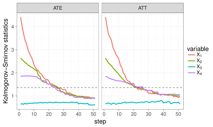
Figure 2. Boosting with $1$-level trees is reducing the maximum Kolmogorov-Smirnov statistics. Two estimands (ATT and ATE) and their corresponding CBSR are considered. Dashed line is the upper $0.05$ quantile of the asymptotic null distribution of the K-S statistic.

As a final remark, the left hand side of (24) or (25) indeed defines a distance metric between two probability distributions (the empirical distributions of the covariates over treatment and control). This distance is called integral probability metric (Müller, 1997) and has received increasing attention recently in the two-sample testing literature. In particular, a very successful multivariate two-sample test (Gretton et al., 2012) uses the left hand side of (25) as its test statistic. Here we have given an alternative statistical motivation of considering the integral probabability metric.

5.4. A Bayesian interpretation

Besides the maximum bias interpretation (25), the RKHS model in Section 4.3 has another interesting Bayesian interpretation. Suppose the regression function $g_{0}$ is also random and generated from a Gaussian random field prior $g_{0}(\cdot)\sim\mathcal{G}(0,K)$ with mean function $0$ and covariance function $K(\cdot,\cdot)$. Then the design MSE of $\hat{\tau}^{*}$ (conditional on $\{X_{i},T_{i}\}_{i=1}^{n}$) under constant treatment effect is given by

$$\begin{split}&\mathrm{E}_{g}\Big{[}\sum_{T_{i}=1}w_{i}g_{0}(X_{i})-\sum_{T_{i}=0}w_{i}g_{0}(X_{i})\Big{]}^{2}+\sum_{i=1}^{n}w_{i}^{2}\mathrm{Var}(Y_{i}|X_{i},T_{i})\\ =&\tilde{w}^{T}K\tilde{w}+\sum_{i=1}^{n}w_{i}^{2}\mathrm{Var}(Y_{i}|X_{i},T_{i}),\end{split}$$

where $\tilde{w}_{i}=(2T_{i}-1)w_{i}$, $i=1,\dotsc,n$ and (with some abuse of notation) $K$ is the sample covariance matrix $K_{ij}=K(X_{i},X_{j})$, $i,j=1,\dotsc,n$. This is directly tied to the dual problem of CBSR maximization. For example, when the estimand is ATT and the link is logistic, using the “kernel trick” $\hat{f}(X_{i})=K\hat{\gamma}$ described in Section 4.3 it is not difficult to show the dual problem minimizes $\lambda\tilde{w}^{T}K\tilde{w}+\sum_{i=1}^{n}w_{i}\log w_{i}$. Choosing different penalty parameters $\lambda$ essentially amounts to different prior beliefs about the conditional variance $\mathrm{Var}(Y|X,T)$. We will explore this Bayesian interpretation in a simulation example in Section 6.

In practice, optimally choosing the regularization parameter $\lambda$ is essentially difficult as it requires prior knowledge about $\|g_{0}\|_{\mathcal{H}_{K}}$ and the conditional variance of $Y$ (essentially the signal-to-noise ratio). Such difficulty exists in all previous approaches and we only attempt to provide a reasonable solution here. Our experience with the adaptive procedures in Section 4 is that once $\lambda$ is reasonably small, the further reduction of maximum bias by decreasing $\lambda$ becomes negligible in most cases. Our best recommendation is to plot the curve of the maximum bias versus $\lambda$, and then the user should use her best judgment based on prior knowledge about the outcome regression. To mitigate the problem of choosing $\lambda$, next we describe how to make valid statistical inference with an arbitrarily chosen $\lambda$.

5.5. Design-based finite-sample inference of WATE

When the treatment effect is not homogeneous, the derivation above no longer holds in general, although the bias-variance trade-off is still expected if the effect is not too inhomogeneous. One exception is when the estimand is ATT. In this case, if the weights are normalized so $w_{i}=1$ if $T_{i}=1$, the finite sample bias of $\hat{\tau}^{*}$ is

$$\begin{split}&\Big{[}\sum_{T_{i}=1}w_{i}g_{1}(X_{i})-\sum_{T_{i}=0}w_{i}g_{0}(X_{i})\Big{]}-\frac{1}{n_{1}}\Big{[}\sum_{T_{i}=1}g_{1}(X_{i})-g_{0}(X_{i})\Big{]}\\ =&\Big{[}\sum_{T_{i}=1}w_{i}g_{0}(X_{i})-\sum_{T_{i}=0}w_{i}g_{0}(X_{i})\Big{]}.\end{split}$$

Therefore, the bias of $\hat{\tau}^{*}$ is only determined by how well $w$ balances $g_{0}$. This fact was noticed in Zhao and Percival (2016), Athey et al. (2016), Kallus (2016) and will be used to construct honest confidence interval for the ATT.

To derive design-based inference of WATE, we assume strong ignorability (Assumption 1) and $Y_{i}\sim\mathrm{N}(g_{T_{i}}(X_{i}),\sigma^{2})$. The normality assumption is not essential when sample size is large, but the homoskedastic assumption is more difficult to relax. We assume the treatment effect is constant if the estimand is not ATT. The only other assumption we make is

Assumption 2.

$g_{0}(x)$ is in a known RKHS $\mathcal{H}_{K}$.

Let the basis function of $\mathcal{H}_{K}$ be $\{\phi_{1}(x),\phi_{2}(x),\dotsc,\}$ and $g_{0}(x)=\sum_{k=1}^{\infty}\beta_{k}\phi_{k}(x)$. Suppose the propensity score is estimated by the RKHS regression described in Section 4.3. Then by the decomposition (17) and equation (25),

$$|\hat{\tau}^{*}-\tau^{*}|\preceq\lambda\|g_{0}\|_{\mathcal{H}_{K}}\|\hat{f}_{\lambda}\|_{\mathcal{H}_{K}}+\mathrm{N}\Big{(}0,\sigma^{2}\sum_{i=1}^{n}w_{i}^{2}\Big{)},$$

where $\preceq$ means stochastically smaller. Therefore, if we can find an upper-$(\alpha/2)$ confidence limit for $\|g_{0}\|_{\mathcal{H}_{K}}$ (denoted by $\mathrm{CL}(\|g_{0}\|_{\mathcal{H}_{K}},1-\alpha/2)$) and a good estimate of $\sigma$ (denoted by $\hat{\sigma}$), then a $(1-\alpha)$-confidence interval of $\tau^{*}$ is given by

$$\hat{\tau}^{*}\pm\big{[}\lambda\|\hat{f}_{\lambda}\|_{\mathcal{H}_{K}}\cdot\mathrm{CL}(\|g_{0}\|_{\mathcal{H}_{K}},1-\alpha/2)+\hat{\sigma}\|w\|_{2}z_{1-\alpha/2}\big{]},$$ (26)

where $z_{1-\alpha/2}$ is the upper-$(\alpha/2)$ quantile of the standard normal distribution. This inferential method can be further extended when an outcome regression adjustment is used (see Section 4.5) by replacing $g_{0}$ with $g_{0}-\hat{g}_{0}$. Notice that in this case $\hat{g}_{0}$ and $\|\hat{g}_{0}\|_{\mathcal{H}_{K}}$ should be estimated using independent sample in order to maintain validity of (26).

Note that our Assumption 2 also covers the setting where $X$ is high dimensional ($d\gg n$) and $g_{0}(x)=\sum_{k=1}^{d}\beta_{k}X_{k}$. In this case, estimating $\|g_{0}\|_{\mathcal{H}_{K}}=\|\beta\|_{2}^{2}$ is of high interest in genetic heritability and we shall use a recent proposal by Janson et al. (2016) in our numeric example below. Estimating $\|g_{0}\|_{\mathcal{H}_{K}}$ when $X$ is low-dimensional can be done in a similar manner by weighting the coefficients.

Athey et al. (2016) considered the inference of ATT when $X$ is high dimensional, but a crucial assumption they require is that $\beta$ is a very sparse vector so that $g_{0}$ can be accurately estimated by lasso regression. In this case, $\lambda\|\hat{g}_{0}-g_{0}\|_{\mathcal{H}_{K}}\|\hat{f}_{\lambda}\|_{\mathcal{H}_{K}}$ is negligible if $\lambda$ is carefully chosen. Our confidence interval above does not require the sparsity assumption since the procedure in Janson et al. (2016) does not need sparsity. Balancing functions in a kernel space is also considered in Hazlett (2016) and Kallus (2016), but they did not consider the statistical inference of weighted average treatment effects.

6. Numerical Examples

This Section provide two simulation examples to demonstrate the flexibility of the proposed framework.

6.1. Simulation: low-dimensional covariates

To illustrate the bias-variance trade-off in selecting model space and regularization parameter, in the following simulation we use a random regression function instead of a manually selected regression function to generate outcome observations. This is motivated by the Bayesian interpretation in Section 5.3. We believe this novel simulation design also better reflects the philosophy of design-based causal inference—the weights generated by the estimated propensity score should be robust against any reasonable outcome regression function.

In this simulation, we consider propensity score models fitted using six kernels: the Gaussian kernel $k(x,x^{\prime})=\exp(-\sigma\|x-x^{\prime}\|^{2})$ with $\sigma=0.1$ or $1$, the Laplace kernel $k(x,x^{\prime})=\exp(-\sigma\|x-x^{\prime}\|)$ with $\sigma=0.1$ or $1$, and the polynomial kernel $k(x,x^{\prime})=(x^{T}x^{\prime}+0.5)^{d}$ with $d=1$ or $3$. Note that in Gaussian and Laplace kernels, smaller $\sigma$ indicates more smoothness. The sample size is $n=1000$ and the covariates are generated by $X_{i}\overset{\mathrm{i.i.d.}}{\sim}\mathrm{N}(0,I_{5})$. The true propensity score is a random function generated by $\mathrm{logit}(P(T=1|X=x))=f(x)\sim\mathcal{G}(0,K(\cdot,\cdot))$ where the covariance function is either the polynomial kernel with degree $1$ or the Gaussian kernel with $\sigma=0.1$. Potential outcomes are generated from the sharp null model $Y_{i}(0)=Y_{i}(1)=g_{0}(X_{i})+\epsilon_{i}$ where $g_{0}(X_{i})$ is a random function generated by the same Gaussian process with any of the six considered kernels. Note that for Gaussian and Laplace kernels, smaller $\sigma$ indicates smoother random functions. For the polynomial kernels, a randomly generated function is just a linear or cubic function with random coefficients.

For choosing the regularization parameter $\lambda$, we stop the RKHS regression described in Section 4.3 when the coefficient of variation of $w$ is less than $0.5$ (“stop early” in the table) or less than $1.2$ (“stop late” in the table). We consider two estimators, the weighted difference estimator with no outcome adjustment (IPW in the table) or with adjustment by outcome regression that is fitted by kernel least squares (same kernel in estimating the propensity score) and tuned by cross-validation (AIPW in the table).

Table 2 reports the average absolute bias over 100 simulations of the two estimators under different simulation settings and propensity score models. Some observations from this table:

1. Under all settings, the lowest bias is always achieved when the fitting kernel is the same kernel that generates the outcome regression function $g_{0}$. This is expected from our Bayesian interpretation in Section 5.4.

2. Outcome adjustment is very helpful when the propensity score estimation is stopped early (so the covariates are less balanced), but makes little improvement when the propensity score estimation is stopped late.

3. There is no uniformly best performing kernel in fitting the propensity score. In particular, polynomial kernels perform poorly when $g_{0}$ is not a polynomial. Laplace kernel with $\sigma=0.1$ performs relatively well in most of the simulation settings.

4. Surprisingly, the kernel used to generate $f$ (logit of the true propensity score) does not alter the qualitative conclusions above. Even if the “correct” kernel is used to fit the propensity score model, there is no guarantee that this better reduces the average bias than other “incorrect” kernels. For example, when $f$ is simulated from poly($d=1$), i.e. $f$ is a random linear function, using the linear propensity score model performs poorly unless $g_{0}$ is also a linear function.

In Section 7, we discuss the practical implications of this simulation result in more detail.

Table 2. Simulation: low-dimensional covariates. Reported numbers are average absolute bias over $100$ simulations.

$f$		poly($d=1$)				gau($\sigma=0.1$)
$\lambda$		stop early		stop late		stop early		stop late
$g_{0}$	fitting kernel	IPW	AIPW	IPW	AIPW	IPW	AIPW	IPW	AIPW
lap($\sigma=0.1$)	lap($\sigma=0.1$)	$0.58$	$0.32$	$0.16$	$0.15$	$0.48$	$0.30$	$0.20$	$0.20$
	lap($\sigma=1$)	$0.59$	$0.39$	$0.24$	$0.24$	$0.50$	$0.30$	$0.22$	$0.22$
	poly($d=1$)	$0.60$	$0.41$	$0.21$	$0.22$	$0.50$	$0.33$	$0.29$	$0.29$
	poly($d=3$)	$0.63$	$0.40$	$0.25$	$0.24$	$0.55$	$0.37$	$0.25$	$0.25$
	gau($\sigma=0.1$)	$0.59$	$0.34$	$0.20$	$0.21$	$0.48$	$0.31$	$0.24$	$0.24$
	gau($\sigma=1$)	$0.62$	$0.50$	$0.35$	$0.35$	$0.58$	$0.41$	$0.29$	$0.30$
lap($\sigma=1$)	lap($\sigma=0.1$)	$0.78$	$0.49$	$0.46$	$0.46$	$0.65$	$0.39$	$0.43$	$0.43$
	lap($\sigma=1$)	$0.79$	$0.48$	$0.43$	$0.43$	$0.64$	$0.40$	$0.38$	$0.38$
	poly($d=1$)	$0.80$	$0.61$	$0.52$	$0.52$	$0.69$	$0.51$	$0.50$	$0.50$
	poly($d=3$)	$0.84$	$0.58$	$0.58$	$0.58$	$0.72$	$0.46$	$0.51$	$0.51$
	gau($\sigma=0.1$)	$0.78$	$0.50$	$0.56$	$0.56$	$0.65$	$0.38$	$0.52$	$0.52$
	gau($\sigma=1$)	$0.80$	$0.56$	$0.50$	$0.51$	$0.66$	$0.50$	$0.41$	$0.42$
poly($d=1$)	lap($\sigma=0.1$)	$1.42$	$0.34$	$0.10$	$0.08$	$1.21$	$0.22$	$0.07$	$0.06$
	lap($\sigma=1$)	$1.47$	$0.69$	$0.46$	$0.46$	$1.33$	$0.47$	$0.35$	$0.34$
	poly($d=1$)	$1.39$	$0.18$	$0.04$	$0.00$	$1.11$	$0.14$	$0.00$	$0.00$
	poly($d=3$)	$1.46$	$0.47$	$0.10$	$0.05$	$1.29$	$0.36$	$0.03$	$0.03$
	gau($\sigma=0.1$)	$1.44$	$0.40$	$0.14$	$0.10$	$1.22$	$0.27$	$0.07$	$0.07$
	gau($\sigma=1$)	$1.60$	$1.17$	$0.82$	$0.83$	$1.50$	$0.89$	$0.66$	$0.64$
poly($d=3$)	lap($\sigma=0.1$)	$1.16$	$0.48$	$0.31$	$0.30$	$0.94$	$0.45$	$0.32$	$0.31$
	lap($\sigma=1$)	$1.25$	$0.66$	$0.53$	$0.53$	$0.98$	$0.54$	$0.48$	$0.48$
	poly($d=1$)	$1.17$	$0.64$	$0.57$	$0.56$	$0.98$	$0.74$	$0.73$	$0.73$
	poly($d=3$)	$1.15$	$0.34$	$0.17$	$0.09$	$0.92$	$0.34$	$0.06$	$0.03$
	gau($\sigma=0.1$)	$1.18$	$0.44$	$0.26$	$0.22$	$0.95$	$0.42$	$0.23$	$0.21$
	gau($\sigma=1$)	$1.32$	$1.02$	$0.79$	$0.79$	$1.04$	$0.76$	$0.63$	$0.63$
gau($\sigma=0.1$)	lap($\sigma=0.1$)	$0.89$	$0.34$	$0.16$	$0.15$	$0.81$	$0.35$	$0.12$	$0.12$
	lap($\sigma=1$)	$0.95$	$0.40$	$0.27$	$0.27$	$0.81$	$0.39$	$0.19$	$0.19$
	poly($d=1$)	$0.92$	$0.46$	$0.37$	$0.37$	$0.85$	$0.58$	$0.51$	$0.51$
	poly($d=3$)	$0.95$	$0.42$	$0.22$	$0.20$	$0.83$	$0.41$	$0.18$	$0.18$
	gau($\sigma=0.1$)	$0.90$	$0.36$	$0.12$	$0.11$	$0.80$	$0.31$	$0.07$	$0.08$
	gau($\sigma=1$)	$0.99$	$0.62$	$0.45$	$0.45$	$0.84$	$0.57$	$0.34$	$0.33$
gau($\sigma=1$)	lap($\sigma=0.1$)	$0.59$	$0.60$	$0.48$	$0.49$	$0.64$	$0.57$	$0.44$	$0.46$
	lap($\sigma=1$)	$0.57$	$0.49$	$0.42$	$0.42$	$0.62$	$0.53$	$0.45$	$0.46$
	poly($d=1$)	$0.59$	$0.58$	$0.58$	$0.58$	$0.64$	$0.64$	$0.62$	$0.62$
	poly($d=3$)	$0.62$	$0.56$	$0.65$	$0.66$	$0.65$	$0.62$	$0.55$	$0.57$
	gau($\sigma=0.1$)	$0.58$	$0.61$	$0.60$	$0.63$	$0.62$	$0.63$	$0.64$	$0.67$
	gau($\sigma=1$)	$0.55$	$0.46$	$0.41$	$0.41$	$0.60$	$0.53$	$0.42$	$0.43$

6.2. Simulation: high-dimensional covariates

In our second example, we consider the case that the covariates $X$ are high dimensional. In this simulation, the sample size $n=1000$ and $X_{i}\in\mathbb{R}^{100}\overset{\mathrm{i.i.d.}}{\sim}\mathrm{N}(0,\Sigma)$ where $\Sigma_{ij}=0.5^{|i-j|}$. The true propensity score is $\mathrm{logit}(P(T_{i}=1|X_{i}))=\rho X_{i}^{T}\theta$ where $\rho=1~{}\mathrm{or}~{}2$, $\theta$ is a $100$-dimensional vector whose first $s_{t}$ entries are $1/\sqrt{s_{t}}$ and the rest are zero, and $s_{t}=5~{}\mathrm{or}~{}100$. The potential outcomes are generated from the sharp null model $Y_{i}(0)=Y_{i}(1)=X_{i}^{T}\beta+\epsilon_{i}$, where the first $s_{y}$ entries of $\beta$ are $1/\sqrt{s_{y}}$ and the rest are zero, $s_{y}=5,~{}20,~{}\mathrm{or}~{}100$, and $\epsilon_{i}$ is an independent Gaussian noise with standard deviation $\sigma=5$.

In this simulation, the propensity score model is fitted by maximizing the CBSR corresponding to ATT ($\alpha=0$, $\beta=-1$) with ridge penalty. The regularization parameter $\lambda$ is chosen so that the coefficient of variation of the weights is just below $1$. Three estimators are considered: the weighted difference estimator with no outcome adjustment (IPW), outcome adjustment fitted by the lasso (AIPW-L), and outcome adjustment fitted by the ridge regression (AIPW-R). The outcome regressions, either fitted by the lasso or the ridge penalty, are tuned by cross-validation.

Averaging over $1000$ simulations, we report in Table 3 the root-mean-square error of the estimators (RMSE), the absolute bias (Bias), the estimated maximum bias as described in Section 5.5 which uses the EigenPrism method of Janson et al. (2016) to estimate $\|\beta\|_{2}$ (Max Bias), coverage of the 95%-confidence interval ignoring covariate imbalance as in Athey et al. (2016) (CI), coverage of the honest 95%-confidence interval (26) (Honest CI), and the ratio of the length between the two confidence intervals (CI Ratio).

Different from the simulation with low-dimensional covariates in Section 6.1, outcome regression adjustment improves estimation accuracy quite significantly. As expected, when $\theta$ is dense ridge outcome regression performs better and when $\theta$ is sparse lasso outcome regression performs better. In many settings, the actual bias is a substantial portion of the estimated maximum bias. Ignoring this bias in the construction of confidence interval can lead to serious under-coverage of the causal parameter, as indicated by the CI column in Table 3. Note that the sparsity assumption in Athey et al. (2016) requires $s_{y}\ll\sqrt{n}/\log(d)\approx 6.9$, so the lack of coverage does not violate the theoretical results in Athey et al. (2016) as the smallest $s_{y}$ in this simulation is $5$. Using the honest confidence interval derived in Section 5.5 ensures the desired coverage, although the confidence interval is a few times wider and quite conservative as expected.

Table 3. Simulation: high-dimensional covariates. Reported values are the average RMSE, average absolute bias, average estimated maximum bias, coverage of the confidence interval ignoring bias due to inexact balance, coverage of the honest confidence interval proposed in Section 5.5, and the average ratio between the two confidence intervals over $1000$ simulations.

$s_{y}$	$\rho$	$s_{t}$	Method	RMSE	Bias	Max Bias	CI	Honest CI	CI Ratio
100	1	100	IPW	$1.41$	$1.35$	$1.47$	$0.12$	$0.99$	$6.00$
			AIPW-L	$1.30$	$1.21$	$1.55$	$0.23$	$0.99$	$6.08$
			AIPW-R	$1.22$	$1.11$	$1.44$	$0.30$	$0.99$	$5.96$
		5	IPW	$0.51$	$0.28$	$1.41$	$0.88$	$1.00$	$5.84$
			AIPW-L	$0.52$	$0.25$	$1.58$	$0.87$	$0.98$	$5.95$
			AIPW-R	$0.51$	$0.21$	$1.32$	$0.87$	$0.98$	$5.66$
	2	100	IPW	$0.91$	$0.78$	$1.02$	$0.49$	$1.00$	$4.40$
			AIPW-L	$0.83$	$0.66$	$1.10$	$0.57$	$1.00$	$4.46$
			AIPW-R	$0.76$	$0.57$	$0.98$	$0.65$	$1.00$	$4.34$
		5	IPW	$0.42$	$0.10$	$0.59$	$0.96$	$0.99$	$2.96$
			AIPW-L	$0.43$	$0.09$	$0.67$	$0.95$	$0.98$	$3.00$
			AIPW-R	$0.43$	$0.07$	$0.55$	$0.96$	$0.98$	$2.88$
20	1	100	IPW	$0.71$	$0.60$	$1.53$	$0.74$	$1.00$	$6.12$
			AIPW-L	$0.62$	$0.43$	$1.61$	$0.82$	$1.00$	$6.13$
			AIPW-R	$0.63$	$0.44$	$1.44$	$0.82$	$1.00$	$5.95$
		5	IPW	$0.78$	$0.64$	$1.42$	$0.62$	$1.00$	$5.86$
			AIPW-L	$0.71$	$0.51$	$1.47$	$0.69$	$0.99$	$5.85$
			AIPW-R	$0.66$	$0.45$	$1.36$	$0.75$	$0.99$	$5.71$
	2	100	IPW	$0.53$	$0.34$	$0.96$	$0.87$	$1.00$	$4.38$
			AIPW-L	$0.49$	$0.24$	$1.01$	$0.90$	$0.98$	$4.37$
			AIPW-R	$0.49$	$0.24$	$0.91$	$0.89$	$0.99$	$4.26$
		5	IPW	$0.48$	$0.22$	$0.56$	$0.93$	$0.99$	$2.94$
			AIPW-L	$0.47$	$0.16$	$0.59$	$0.94$	$0.99$	$2.93$
			AIPW-R	$0.46$	$0.15$	$0.52$	$0.94$	$0.99$	$2.88$
5	1	100	IPW	$0.51$	$0.29$	$1.59$	$0.90$	$0.99$	$6.17$
			AIPW-L	$0.49$	$0.18$	$1.55$	$0.92$	$0.98$	$6.02$
			AIPW-R	$0.52$	$0.23$	$1.54$	$0.89$	$0.98$	$6.04$
		5	IPW	$1.24$	$1.19$	$1.27$	$0.17$	$0.99$	$5.73$
			AIPW-L	$1.05$	$0.91$	$1.29$	$0.39$	$0.99$	$5.75$
			AIPW-R	$1.09$	$0.99$	$1.26$	$0.33$	$1.00$	$5.72$
	2	100	IPW	$0.43$	$0.17$	$0.98$	$0.94$	$0.99$	$4.44$
			AIPW-L	$0.42$	$0.10$	$0.93$	$0.94$	$0.99$	$4.34$
			AIPW-R	$0.43$	$0.13$	$0.92$	$0.93$	$0.99$	$4.35$
		5	IPW	$0.61$	$0.43$	$0.54$	$0.82$	$1.00$	$2.93$
			AIPW-L	$0.55$	$0.29$	$0.53$	$0.88$	$0.99$	$2.91$
			AIPW-R	$0.56$	$0.33$	$0.53$	$0.87$	$1.00$	$2.91$

7. Discussion

We have proposed a general method of obtaining covariate balancing propensity score which unifies many previous approaches. Our proposal is conceptually simple: the investigator just needs to tailor the loss function according to the link function and estimand. This offers great flexibility in incorporating adaptive strategies developed in statistical learning. We have given a through discourse on the dual interpretation of minimizing the tailored loss function, especially how regularization is linked to the bias-variance trade-off in estimating the weighted average treatment effects. We provide honest inference that account for the bias incurred by inexact balance.

Throughout the paper we have taken an outright design perspective: without looking at the outcome data, the investigator tries to balance pre-treatment covariates as well as possible to mimic a randomized experiment, echoing the recommendations by Rubin (2008, 2009). This allows us to give an interesting Bayesian interpretation of covariate balance: when checking covariate imbalance and deciding which propensity score model is “acceptable”, the investigator is implicitly assuming a prior on the unknown outcome regression function.

The conclusions from the simulation examples in Section 6 are quite intricate and it stresses an essential difficulty in observational studies: no design is uniformly the best (unless the observations can be exactly matched). The investigator must be aware that weaker modeling assumption ($g_{0}$ is in a larger function space) leads to wider confidence interval of the causal effect, and any statistical inference is relative to this assumption. In practice, when the covariate dimension is low we recommend using a universal kernel (such as Gaussian or Laplace kernel, see e.g. Gretton et al. (2012)) to estimate the propensity score, so the model space is dense in the space of continuous functions. We encourage the user to try different kernels (e.g. Laplace kernel with different $\sigma$) and report how the confidence interval changes with different modeling assumption. This shows how sensitive the statistical inference is to the modeling assumption. When the covariate dimension is high and a linear outcome model is assumed, our simulation results suggest that the user should be cautious about any further sparsity assumption that eliminates the bias due to inexact balance. Honest confidence interval can be constructed without the sparsity assumption, but the interval can also be too wide if the covariate dimension is much larger than the sample size.

Appendix A Technical proofs

A.1. Proof of Proposition 2

The same result can be found in Buja et al. (2005, Section 15). For completeness we give a direct proof here. Denote $p=l^{-1}(f)\in(0,1)$. Since $v=v_{\alpha,\beta}$, we have

$$\frac{G^{\prime\prime}(p)}{l^{\prime}(p)}=p^{\alpha}(1-p)^{\beta}$$

Therefore, by the chain rule and the inverse function theorem,

$$\begin{split}\frac{\mathrm{d}}{\mathrm{d}f}S(l^{-1}(f),1)&=(1-p)G^{\prime\prime}(p)(l^{-1})^{\prime}(f)=p^{\alpha}(1-p)^{\beta+1},\\ \frac{\mathrm{d}}{\mathrm{d}f}S(l^{-1}(f),0)&=-pG^{\prime\prime}(p)(l^{-1})^{\prime}(f)=-p^{\alpha+1}(1-p)^{\beta},~{}\mathrm{and}\end{split}$$

$$\begin{split}\frac{\mathrm{d}^{2}}{\mathrm{d}f^{2}}S(l^{-1}(f),1)&=\alpha p^{\alpha}(1-p)^{\beta+2}-(\beta+1)p^{\alpha+1}(1-p)^{\beta+1},\\ \frac{\mathrm{d}^{2}}{\mathrm{d}f^{2}}S(l^{-1}(f),0)&=-(\alpha+1)p^{\alpha+1}(1-p)^{\beta+1}+\beta p^{\alpha+2}(1-p)^{\beta}.\end{split}$$

The conclusions immediate follow by letting the second order derivatives be less than or equal to $0$.

A.2. Proof of Theorem 2

First we list the technical assumptions in Hirano et al. (2003):

Assumption 3.

(Distribution of ${X}$) The support of ${X}$ is a Cartesian product of compact intervals. The density of ${X}$ is bounded, and bounded away from $0$.

Assumption 4.

(Distribution of $Y(0),~{}Y(1)$) The second moments of $Y(0)$ and $Y(1)$ exist and $g({X},0)=\mathrm{E}[Y(0)|{X}]$ and $g({X},1)=\mathrm{E}[Y(1)|{X}]$ are continuously differentiable.

Assumption 5.

(Propensity score) The propensity score $p({X})=\mathrm{P}(T=1|{X})$ is continuously differentiable of order $s\geq 7d$ where $d$ is the dimension of ${X}$, and $p({x})$ is bounded away from $0$ and $1$.

Assumption 6.

(Sieve estimation) The nonparametric sieve logistic regression uses a power series with $m=n^{\nu}$ for some $1/(4(s/d-1))<\nu<1/9$.

The proof is a simple modification of the proof in Hirano et al. (2003). In fact, Hirano et al. (2003) only proved the convergence of the estimated propensity score up to certain order. This essentially suggests that the semiparametric efficiency of $\hat{\tau}$ does not heavily depend on the accuracy of the sieve logistic regression.

To be more specific, only three properties of the maximum likelihood rule $S=S_{0,0}$ are used in Hirano et al. (2003, Lemmas 1,2):

1. $\tilde{{\theta}}=\arg\max_{{\theta}}S(p_{{\theta}},p_{\tilde{{\theta}}})$ (line 5, page 19), this is exactly the definition of a strictly proper scoring rule (1);

2. The Fisher information matrix

   $$\frac{\partial^{2}}{\partial{\theta}\partial{\theta}^{T}}S(p_{{{\theta}}},p_{\tilde{{\theta}}})=\mathrm{E}_{\tilde{{\theta}}}\left\{\left[\frac{\mathrm{d}^{2}}{\mathrm{d}f^{2}}S(l^{-1}(f),T)\Bigr{|}_{f={\phi}({X})^{T}{{\theta}}}\right]{\phi}({X}){\phi}({X})^{T}\right\}$$

   has all eigenvalues uniformly bounded away from $0$ for all ${\theta}$ and $\tilde{{\theta}}$ in a compact set in $\mathbb{R}^{m}$, where the expectation on the right hand side is taken over ${X}$ and $T|{X}\sim p_{\tilde{{\theta}}}$.

3. As $m\to\infty$, with probability tending to $1$ the observed Fisher information matrix

   $$\frac{\partial^{2}}{\partial{\theta}\partial{\theta}^{T}}\frac{1}{n}\sum_{i=1}^{n}S(p_{{{\theta}}}({X}_{i}),T_{i})=\frac{1}{n}\sum_{i=1}^{n}\left[\frac{\mathrm{d}^{2}}{\mathrm{d}f^{2}}S(l^{-1}(f),T_{i})\Bigr{|}_{f={\phi}({X}_{i})^{T}{{\theta}}}\right]{\phi}({X}_{i}){\phi}({X}_{i})^{T}$$

   has all eigenvalues uniformly bounded away from $0$ for all ${{\theta}}$ in a compact set of $\mathbb{R}^{m}$ (line 7–9, page 21).

Because the approximating functions ${\phi}$ are obtained through orthogonalizing the power series, we have $\mathrm{E}[{\phi}({X}){\phi}({X})^{T}]={I}_{m}$ and one can show its finite sample version has eigenvalues bounded away from $0$ with probability going to $1$ as $n\to\infty$. Therefore a sufficient condition for the second and third properties above is that $S(l^{-1}(f),t)$ is strongly concave for $t=0,1$. In Proposition 2 we have already proven the strong concavity for all $-1\leq\alpha,\beta\geq 1$ except for $\alpha=-1,\beta=0$ and $\alpha=0,\beta=-1$. In these two boundary cases, among $S(l^{-1}(f),0)$ and $S(l^{-1}(f),1)$ one score function is strongly concave and the other score function is linear in $f$. One can still prove the second and third properties by using Assumption 5 that the propensity score is bounded away from $0$ and $1$.

A.3. Proof of Proposition 3

The conclusion is trivial for $a=1$. Denote

$$h(f,t)=\frac{\mathrm{d}}{\mathrm{d}f}S(l^{-1}(f),t)~{}\mathrm{and}~{}h^{\prime}(f,t)=\frac{\mathrm{d}}{\mathrm{d}f}h(f,t),~{}t=0,1.$$

Because $S(l^{-1}(f),t)$ is concave in $f$, we have $h^{\prime}(f,t)<0$ for all $f$. The first-order optimality condition of (14) is given by

$$\frac{1}{n}\sum_{i=1}^{n}h(\hat{\theta}_{\lambda}^{T}{\phi}({X}_{i}),T_{i}){\phi}_{k}({X}_{i})+\lambda|(\hat{\theta}_{\lambda})_{k}|^{a-1}\mathrm{sign}((\hat{\theta}_{\lambda})_{k})=0,~{}k=1,\dotsc,m.$$

Let $\nabla\hat{\theta}_{\lambda}$ be the gradient of $\hat{\theta}_{\lambda}$ with respect to $\lambda$. By taking derivative of the identity above, we get

$$\left[\frac{1}{n}\sum_{i=1}^{n}h^{\prime}(\hat{\theta}_{\lambda}^{T}{\phi}_{i},T_{i})\phi_{i}\phi_{i}^{T}+\lambda(a-1)\mathrm{diag}(|\hat{\theta}_{\lambda}|^{a-2})\right]\nabla\hat{\theta}_{\lambda}=-|\hat{\theta}_{\lambda}|^{a-1}\mathrm{sign}(\hat{\theta}_{\lambda}),$$

where we used the abbreviation $\phi_{i}=\phi(X_{i})$ and $\theta^{a}=(\theta_{1}^{a},\dotsc,\theta_{m}^{a})$. For brevity, let’s denote

$$H=\frac{1}{n}\sum_{i=1}^{n}h^{\prime}(\hat{\theta}_{\lambda}^{T}{\phi}_{i},T_{i})\phi_{i}\phi_{i}^{T}\prec 0~{}\mathrm{and}~{}G=\lambda(a-1)\mathrm{diag}(|\hat{\theta}_{\lambda}|^{a-2}).$$

For $a>1$, the result is proven by showing the derivative of $\lambda\|\hat{\theta}_{\lambda}\|_{a}^{a-1}$ is greater than $0$.

$$\begin{split}\frac{\mathrm{d}}{\mathrm{d}\lambda}\left(\lambda\|\hat{\theta}_{\lambda}\|_{a}^{a-1}\right)&=\|\hat{\theta}_{\lambda}\|_{a}^{a-1}+\lambda\frac{\mathrm{d}}{\mathrm{d}\lambda}\Bigg{[}\sum_{j=1}^{m}\left|(\hat{\theta}_{\lambda})_{k}\right|^{a}\Bigg{]}^{(a-1)/a}\\ &=\|\hat{\theta}_{\lambda}\|_{a}^{a-1}+\lambda(a-1)\|\hat{\theta}_{\lambda}\|_{a}^{-1}\sum_{j=1}^{m}\left|(\hat{\theta}_{\lambda})_{k}\right|^{a-1}(\nabla\hat{\theta}_{\lambda})_{k}\,\mathrm{sign}((\hat{\theta}_{\lambda})_{k})\\ &=\|\hat{\theta}_{\lambda}\|_{a}^{a-1}-\lambda(a-1)\|\hat{\theta}_{\lambda}\|_{a}^{-1}(|\hat{\theta}_{\lambda}|^{a-1})^{T}(H+G)^{-1}|\hat{\theta}_{\lambda}|^{a-1}\\ &>\|\hat{\theta}_{\lambda}\|_{a}^{a-1}-\lambda(a-1)\|\hat{\theta}_{\lambda}\|_{a}^{-1}(|\hat{\theta}_{\lambda}|^{a-1})^{T}G^{-1}|\hat{\theta}_{\lambda}|^{a-1}\\ &=0.\end{split}$$

Appendix B A closer look at the Beta family

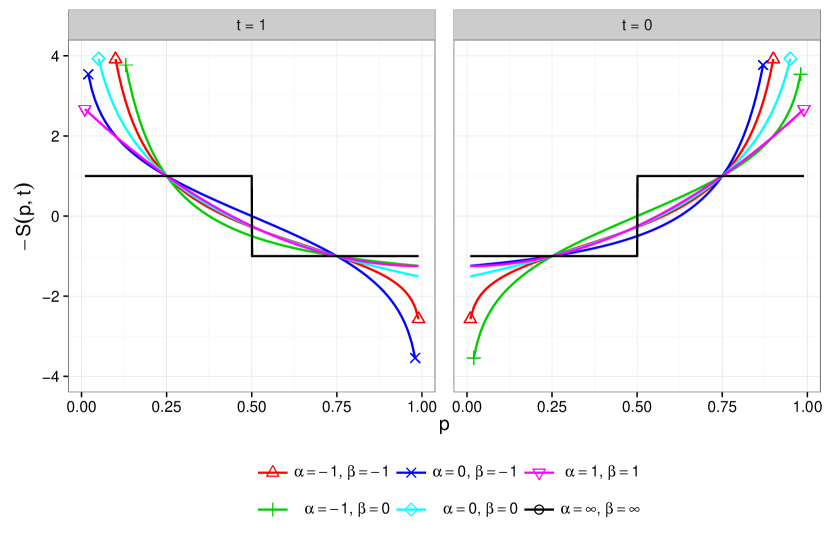
(a) Loss functions $-S_{\alpha,\beta}(p,t)$ for $t=0,1$.

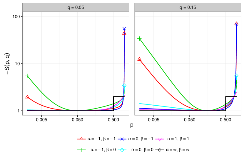
(b) Loss functions $-S_{\alpha,\beta}(p,q)$ for $q=0.05$ and $0.15$.

Figure 3. Graphical illustration of the Beta-family of scoring rules defined in (3).

Figure 3 plots the scoring rules $S_{\alpha,\beta}$ for some combinations of $\alpha$ and $\beta$. The top panels show the score function $S(p,0)$ and $S(p,1)$ for $0<p<1$, which are normalized so that $S(1/4,1)=S(3/4,0)=-1$ and $S(1/4,0)=S(3/4,1)=1$. By a change of variable, one can show $S_{\alpha,\beta}(p,1)=S_{\beta,\alpha}(1-p,0)$. This is the reason that the two subplots in Figure 3(a) are essentially reflections of each other. The bottom panels show the induced scoring rule $S(p,q)$ defined by section 2.1 or more specifically $S(p,q)=qS(p,1)+(1-q)S(p,0)$ at two different values of $q=0.05,0.15$. For aesthetic purposes, the scoring rules in Figure 3(b) are normalized such that $-S(p,q)=1$ and $-S(p,1-q)=2$.

Figure 3 shows that the scoring rules $S_{\alpha,\beta}$, when $-1\leq\alpha,\beta\leq 0$, are highly sensitive to small differences of small probabilities. For example, in Figure 3(a) the loss function $-S_{\alpha,\beta}(p,1)$ is unbounded above when $\alpha,\beta\in\{-1,0\}$, hence a small change of $p$ near $0$ may have a big impact on the score. In Figure 3(b), the averaged scoring rules $S_{\alpha,\beta}(p,q)$, when $(\alpha,\beta)=(-1,-1)$ or $(-1,0)$, are also unbounded near $p=0$. Due to this reason, selten1998axiomatic argued that these scoring rules are inappropriate for probability forecast problems.

On the contrary, the unboundedness is actually a desirable feature for propensity score estimation, as the goal is to avoid extreme probabilities. Consider the standard inverse probability weights (IPW)

$$\hat{w}_{i}=\begin{cases}\hat{p}_{i}^{-1}&\mathrm{if}~{}T_{i}=1,\\ (1-\hat{p}_{i})^{-1}&\mathrm{if}~{}T_{i}=0,\\ \end{cases}$$ (27)

where $\hat{p}_{i}=p_{\hat{\theta}}(X_{i})$ is the estimated propensity score for the $i$-th data point. This corresponds to $\alpha=\beta=-1$ in the Beta family and estimates ATE. Several previous articles (e.g. Robins2000, Kang and Schafer, 2007, Robins2007) have pointed out the hazards of using large inverse probability weights. For example, if the true propensity score is $p(X_{i})=q=0.05$ and it happens that $T_{i}=1$, we would want $\hat{p}_{i}$ not too close to $0$ so $\hat{w}_{i}$ is not too large. Conversely, we also want $\hat{p}_{i}$ not too close to $1$, so in the more likely event that $T_{i}=0$ the weight $\hat{w}_{i}$ is not too large either. In an ad hoc attempt to mitigate this issue, lee2011weight studied weight truncation (e.g. truncate the largest 10% weights). They found that the truncation can reduce the standard error of the estimator $\hat{\tau}$ but also increases the bias.

The covariate balancing scoring rules provide a more systematic approach to avoid large weights. For example, the scoring rule $S_{-1,-1}$ precisely penalizes large inverse probability weights as $-S_{-1,-1}(p,q)$ is unbounded above when $p$ is near $0$ or $1$ (see the left plot in Figure 3(b)). Similarly, when estimating the ATUT $\tau_{-1,0}$, the weighting scheme would put $\hat{w}_{i}\propto(1-\hat{p}_{i})/\hat{p}_{i}$ if $T_{i}=1$ and $\hat{w}_{i}\propto 1$ if $T_{i}=0$. Therefore we would like $\hat{p}_{i}$ to be not close to $0$, but it is acceptable if $\hat{p}_{i}$ is close to $1$. As shown in in Figure 3(b), the curve $-S_{-1,0}(p,q)=q/p+(1-q)\log(p/(1-p))$ precisely encourages this behavior, as it is unbounded above when $p$ is near $0$ and grows slowly when $p$ is near $1$.

References

- Abadie and Imbens (2006) Abadie, A. and G. W. Imbens (2006). Large sample properties of matching estimators for average treatment effects. Econometrica 74(1), 235–267.
- Athey et al. (2016) Athey, S., G. W. Imbens, S. Wager, et al. (2016). Approximate residual balancing: De-biased inference of average treatment effects in high dimensions. arXiv preprint arXiv:1604.07125.
- Austin and Stuart (2015) Austin, P. C. and E. A. Stuart (2015). Moving towards best practice when using inverse probability of treatment weighting (iptw) using the propensity score to estimate causal treatment effects in observational studies. Statistics in Medicine 34(28), 3661–3679.
- Breiman et al. (1984) Breiman, L., J. Friedman, C. J. Stone, and R. A. Olshen (1984). Classification and regression trees. CRC press.
- Buja et al. (2005) Buja, A., W. Stuetzle, and Y. Shen (2005). Loss functions for binary class probability estimation and classification: Structure and applications. Working draft.
- Caliendo and Kopeinig (2008) Caliendo, M. and S. Kopeinig (2008). Some practical guidance for the implementation of propensity score matching. Journal of Economic Surveys 22(1), 31–72.
- Chan et al. (2016) Chan, K. C. G., S. C. P. Yam, and Z. Zhang (2016). Globally efficient nonparametric inference of average treatment effects by empirical balancing calibration weighting. Journal of Royal Statistical Society, Series B (Methodology) 78(3), 673–700.
- Cochran (1953) Cochran, W. G. (1953). Matching in analytical studies. American Journal of Public Health and the Nations Health 43(6_Pt_1), 684–691.
- Cochran (1968) Cochran, W. G. (1968). The effectiveness of adjustment by subclassification in removing bias in observational studies. Biometrics, 295–313.
- Crump et al. (2006) Crump, R., V. J. Hotz, G. Imbens, and O. Mitnik (2006). Moving the goalposts: Addressing limited overlap in the estimation of average treatment effects by changing the estimand. Technical Report 330, National Bureau of Economic Research.
- Deville and Särndal (1992) Deville, J.-C. and C.-E. Särndal (1992). Calibration estimators in survey sampling. Journal of the American Statistical Association 87(418), 376–382.
- Efron et al. (2004) Efron, B., T. Hastie, I. Johnstone, and R. Tibshirani (2004). Least angle regression. The Annals of Statistics 32(2), 407–499.
- Fan et al. (2016) Fan, J., K. Imai, H. Liu, Y. Ning, and X. Yang (2016). Improving covariate balancing propensity score: A doubly robust and efficient approach. Technical report, Princeton University.
- Friedman et al. (1998) Friedman, J., T. Hastie, and R. Tibshirani (1998). Additive logistic regression: a statistical view of boosting. Annals of Statistics 28, 2000.
- Friedman (2001) Friedman, J. H. (2001). Greedy function approximation: a gradient boosting machine. Annals of statistics, 1189–1232.
- Gneiting and Raftery (2007) Gneiting, T. and A. E. Raftery (2007). Strictly proper scoring rules, prediction, and estimation. Journal of the American Statistical Association 102(477), 359–378.
- Graham et al. (2012) Graham, B. S., C. C. D. X. Pinto, and D. Egel (2012). Inverse probability tilting for moment condition models with missing data. The Review of Economic Studies 79(3), 1053–1079.
- Gretton et al. (2012) Gretton, A., K. M. Borgwardt, M. J. Rasch, B. Schölkopf, and A. Smola (2012). A kernel two-sample test. Journal of Machine Learning Research 13(Mar), 723–773.
- Hainmueller (2011) Hainmueller, J. (2011). Entropy balancing for causal effects: a multivariate reweighting method to produce balanced samples in observational studies. Political Analysis 20, 25–46.
- Hastie et al. (2009) Hastie, T., R. Tibshirani, and J. Friedman (2009). Elements of statistical learning. Springer.
- Hazlett (2016) Hazlett, C. (2016). Kernel balancing: A flexible non-parametric weighting procedure for estimating causal effects. arXiv preprint arXiv:1605.00155.
- Heckman et al. (1997) Heckman, J. J., H. Ichimura, and P. E. Todd (1997). Matching as an econometric evaluation estimator: Evidence from evaluating a job training programme. The Review of conomic Studies 64(4), 605–654.
- Hirano and Imbens (2001) Hirano, K. and G. Imbens (2001). Estimation of causal effects using propensity score weighting: an application to data on right heart catheterization. Health Services and Outcomes Research Methodology 2, 259–278.
- Hirano et al. (2003) Hirano, K., G. W. Imbens, and G. Ridder (2003). Efficient estimation of average treatment effects using the estimated propensity score. Econometrica 71(4), 1161–1189.
- Hofmann et al. (2008) Hofmann, T., B. Schölkopf, and A. J. Smola (2008). Kernel methods in machine learning. The Annals of Statistics, 1171–1220.
- Imai et al. (2008) Imai, K., G. King, and E. A. Stuart (2008). Misunderstandings between experimentalists and observationalists about causal inference. Journal of the Royal Statistical Society: Series A (Statistics in Society) 171(2), 481–502.
- Imai and Ratkovic (2014) Imai, K. and M. Ratkovic (2014). Covariate balancing propensity score. Journal of the Royal Statistical Society: Series B (Statistical Methodology) 76(1), 243–263.
- Imbens (2004) Imbens, G. W. (2004). Nonparametric estimation of average treatment effects under exogeneity: A review. Review of Economics and statistics 86(1), 4–29.
- Imbens and Rubin (2015) Imbens, G. W. and D. B. Rubin (2015). Causal inference for statistics, social, and biomedical sciences. Cambridge University Press.
- Janson et al. (2016) Janson, L., R. F. Barber, and E. Candès (2016). Eigenprism: inference for high dimensional signal-to-noise ratios. Journal of the Royal Statistical Society: Series B (Statistical Methodology).
- Kallus (2016) Kallus, N. (2016). Generalized optimal matching methods for causal inference. arXiv preprint arXiv:1612.08321.
- Kang and Schafer (2007) Kang, J. D. and J. L. Schafer (2007). Demystifying double robustness: a comparison of alternative strategies for estimating a population mean from incomplete data. Statistical Science 22(4), 523–539.
- Li et al. (2016) Li, F., K. L. Morgan, and A. M. Zaslavsky (2016). Balancing covariates via propensity score weighting. Journal of the American Statistical Association to appear.
- Lunceford and Davidian (2004) Lunceford, J. K. and M. Davidian (2004). Stratification and weighting via the propensity score in estimation of causal treatment effects: a comparative study. Statistics in Medicine 23(19), 2937–2960.
- McCullagh and Nelder (1989) McCullagh, P. and J. A. Nelder (1989). Generalized linear models. CRC press.
- Müller (1997) Müller, A. (1997). Integral probability metrics and their generating classes of functions. Advances in Applied Probability 29(02), 429–443.
- Normand et al. (2001) Normand, S.-L. T., M. B. Landrum, E. Guadagnoli, J. Z. Ayanian, T. J. Ryan, P. D. Cleary, and B. J. McNeil (2001). Validating recommendations for coronary angiography following acute myocardial infarction in the elderly: a matched analysis using propensity scores. Journal of clinical epidemiology 54(4), 387–398.
- Robins et al. (1994) Robins, J. M., A. Rotnitzky, and L. Zhao (1994). Estimation of regression coefficients when wome regressors are not always observed. Journal of the American Statistical Association 89, 846–866.
- Rosenbaum and Rubin (1983) Rosenbaum, P. and D. Rubin (1983). The central role of the propensity score in observational studies for causal effects. Biometrika 70(1), 41–55.
- Rosenbaum and Rubin (1984) Rosenbaum, P. and D. Rubin (1984). Reducing bias in observational studies using subclassification on the propensity score. Journal of the American Statistical Association 79, 516–524.
- Rosenbaum and Rubin (1985) Rosenbaum, P. R. and D. B. Rubin (1985). Constructing a control group using multivariate matched sampling methods that incorporate the propensity score. The American Statistician 39(1), 33–38.
- Rubin (1973) Rubin, D. B. (1973). Matching to remove bias in observational studies. Biometrics, 159–183.
- Rubin (2008) Rubin, D. B. (2008). For objective causal inference, design trumps analysis. The Annals of Applied Statistics, 808–840.
- Rubin (2009) Rubin, D. B. (2009). Should observational studies be designed to allow lack of balance in covariate distributions across treatment groups? Statistics in Medicine 28(9), 1420–1423.
- Savage (1971) Savage, L. J. (1971). Elicitation of personal probabilities and expectations. Journal of the American Statistical Association 66(336), 783–801.
- Smith and Todd (2005) Smith, J. A. and P. E. Todd (2005). Does matching overcome lalonde’s critique of nonexperimental estimators? Journal of econometrics 125(1), 305–353.
- Stuart (2010) Stuart, E. A. (2010). Matching methods for causal inference: A review and a look forward. Statistical Science 25(1), 1–21.
- Wahba (1990) Wahba, G. (1990). Spline models for observational data, Volume 59. SIAM.
- Zhao and Percival (2016) Zhao, Q. and D. Percival (2016). Entropy balancing is doubly robust. Journal of Causal Inference to appear.
- Zubizarreta (2015) Zubizarreta, J. R. (2015). Stable weights that balance covariates for estimation with incomplete outcome data. Journal of the American Statistical Association 110(511), 910–922.