Spatial repartition of local plastic processes in different creep regimes in a granular material

Abstract

Granular packings under constant shear stress display below the Coulomb limit, a logarithmic creep dynamics. However the addition of small stress modulations induces a linear creep regime characterized by an effective viscous response. Using Diffusing Wave Spectroscopy, we investigate the relation between creep and local plastic events spatial distribution (“hot-spots”) contributing to the plastic yield. The study is done in the two regimes, i.e. with and without mechanical activation. The hot-spot dynamics is related to the material effective fluidity. We show that far from the threshold, a local visco-elastic rheology coupled to an ageing of the fluidity parameter, is able to render the essential spatio-temporal features of the observed creep dynamics.

Granular solids Deformation, plasticity, and creep Material behavior

1 Introduction

Granular packings are often seen as rigid below a limit corresponding to a critical ratio between shear stress and normal stress (Coulomb threshold) [1]. However, the existence of a clear-cut transition between a solid-like and liquid-like behaviour is currently strongly challenged [2, 3, 4, 5]. In the presence of a shear band (i.e. a fluid zone dwelling somewhere in the packing) different authors brought evidences for mechanically activated creeping processes taking place in remote regions, below the Coulomb threshold[2, 3]. This behaviour led to non-local rheological relations proposed to extend the standard local constitutive relations for granular flows [6, 7, 8, 9]. For granular packing sheared in all of its parts below the Coulomb limit, dynamical processes leading to a logarithmic creep occurs [10, 4, 5]. Interestingly, this creeping dynamics can be mapped onto a simple visco-elastic model initially designed to render the phenomenology of yield stress fluids displaying ageing in the solid phase [11]. The model is centred on a dynamical equation for a fluidity parameter representing an effective visco-elastic relaxation. This phenomenological parameter was directly related to the occurrence of mesoscopic plastic events called ”hot spots” [5]. In the vicinity of the dynamical threshold, these events combine to provide large scale plastic yields [5, 12]. Recently, we have shown that providing a tiny stress modulation around a nominal shear stress, the creep dynamics changes from a logarithmic to a linear behaviour [13]. The physical interpretation stems from the combination of memory effects and non-linearities, leading to a ”secular” accumulation of tiny effects, meaning that the creep dynamics is revealed at a time scale much larger than the modulation. We call this behaviour “rectified creep” in the following as the interpretation of this regime is different from an Eyring-like activated process. As the ingredients at the origin of this rectified creep are generic for a large class of soft glassy materials, this effect should be seen in other yield stress fluids displaying creep [14, 15, 16, 17].

In this paper, using a spatially resolved multiple scattering technique [18], we monitor the spatial distribution of hot-spots during the two creep regimes. In parallel, a spatially resolved visco-elastic model is solved assuming a direct relation between the hot-spots production rate and the local fluidity value. The numerical solution is compared to the experiments. Interpretation of the results in the framework of a local rheological model is provided.

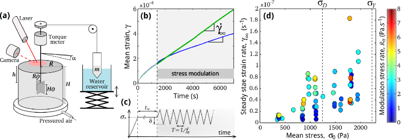
Figure 1: (a) Experimental set-up: shear is imposed by an hanging mass $m$ connected to the vertical axis; vertical displacement of the water reservoir allows modulation of the applied stress; a camera collects backscattered light from a He-Ne laser illuminating the top of the shear cell. (b) Mean strain as a function of time for two experiments performed at $\sigma_{0}=1100Pa$, and $\delta=7.5Pa$ , and for two oscillations frequencies: 0.099 Hz (blue line) and 0.168 Hz (green line). The oscillations start at $t=1500s$ (grey area). $\dot{\gamma}_{\infty}$ is the slope of the linear part. (c) Imposed stress during an experiment: stress ramp to reach mean stress, $\sigma_{0}$, constant stress during $t_{w}$ and stress modulation characterized by a frequency $f_{\sigma}$ and an amplitude $\delta$. (d) Steady state strain rate, $\dot{\gamma}_{\infty}$, as a function of mean stress, $\sigma_{0}$. Color of the symbol stands for the value of modulation stress rate $R_{\sigma}=4\delta f$.

2 Methods

The experimental set-up is shown in fig. 1a. It consists in a cylindrical shear cell (Radius $R=5cm$, height $H=10cm$) filled with glass beads of density $\rho=2500\ kg/m^{3}$ and mean diameter $d=200\ \mu m$ (rms polydispersity $\Delta d=30\ \mu m$). A well defined packing fraction $\Phi=0.605\pm 0.005$ is obtaining using an air fluidized bed as described by Nguyen et al. [4].

Shear is obtained by applying a torque on a stainless steel four-blade vane (radius $R_{0}=1.27\ cm$, height $H_{0}=2.54\ cm$) via a mass $m$ suspended from a pulley (see fig. 1a). Using this “Atwood-machine” technique, mechanical noise inherently coming from any motorized process can be suppressed. The mass $m$ hangs partially inside a reservoir filled with water. Thus, by modulating the Archimedes force, through the up and down motion of the reservoir sitting on a vertical translation stage, controlled modulation of the torque applied to the granular packing can be obtained. A torque probe connected to the vane axis measures the applied torque $T$. The vane rotation angle $\alpha$ is monitored via a transverse arm whose displacement is measured by an induction probe. Torque and displacement signals as well as the vertical translation stage command are connected to a Labview controller board. We defined here the mean stress and the mean strain as $\sigma_{0}=\frac{T}{2\pi R_{0}^{2}H_{0}}$ and $\gamma=\frac{\alpha R_{0}}{R-R_{0}}$ respectively.

For a given experiment, the protocol (fig. 1c) is the following $(i)$ stress ramp at constant stress rate ($\dot{\sigma}=5\ Pa/s$) up to the desired mean stress value $\sigma_{0}$; $(ii)$ constant shear $\sigma_{0}$ applied during $t_{w}=1500\ s$; $(iii)$ modulation of the stress around $\sigma_{0}$ for at least 2 hours. The modulation consist in triangular oscillations with an amplitude $\delta$ and a frequency $f_{\sigma}$. We introduce the modulation stress rate, $R_{\sigma}=4\delta f_{\sigma}$ to characterize the modulation.

Let us note that we used the same set-up and protocol than [13] and results presented here include those already presented. The two following points differs from the former study.

Here, two vane penetration depths were used : $h=5\ cm$ and $0\ cm$. During the vane insertion procedure, in order to prevent large scale disturbances in the packing, pressurized air is gently flown, just below the fluidization threshold providing a packing at the surface bearing almost no confining pressure. In addition, after the introduction of the vane, we kept the air flowing during 10 min in order to relax the remaining stress perturbations induced by the vane insertion. The air flow is switched off before the start of the experiment. For experiments performed with the vane near the surface ($h=0\ cm$), the grains are confined with a glass plate in order to obtain a confining pressure at the top of the vane close to the one existing for experiments done at the insertion height $h=5\ cm$. The circular glass plate has a central hole to let the vane shaft go through and the vertical confinement pressure was adjusted by placing loads on the glass plate.

In addition to the mechanical measurements, we obtain, by diffusive wave spectroscopy (DWS) [18, 19, 5], a spatially resolved map of the top surface deformations. DWS is an interference technique using scattering of coherent light by strongly diffusive materials. In our case, a He-Ne laser ($\lambda=633\ nm$) illuminates the top of the shear cell. A camera imaging the surface at a frame rate of 0.1 Hz collects back-scattered light (fig. 1a). The correlation of scattered intensities between two successive images, $g_{I}$, is computed by zones of 16 $\times$ 16 pixels, composing correlation maps of 370 $\mu m$ resolution. The link between the value of $g_{I}$ and the corresponding deformations that have occurred inside the sample were extensively described in [18, 19]. Maximal correlation ($g_{I}>0.99$, white on Fig. 2a) corresponds to an homogeneous deformation below $10^{-7}$ and vanishing correlation (black on Fig. 2a) corresponds to deformations larger than $10^{-5}$.

3 Experimental results

Figure 1.b shows typical deformations for two experiments performed at the same mean stress ($\sigma_{0}=1100Pa$) and oscillation amplitude ($\delta=7.5Pa$) for two oscillation frequencies. These two experiments were performed at a penetration depth $h=5cm$. During the phase at constant stress, we observe a slow increase of the deformation, $\gamma(t)$, similar for both experiments. This initial dynamics can be fitted by a logarithmic curve as in [4]. Then, when submitted to oscillations, the system transits to a linear creep regime characterized by a constant mean strain rate, $\dot{\gamma}_{\infty}$, which increases with the oscillation frequency. This sub-threshold fluidization by mechanical perturbation has been already reported and interpreted in [13] as a secular drift process. Figure 1.d shows the value of the steady state strain rate, $\dot{\gamma}_{\infty}$, for all the experiments performed at $h=5cm$ and at various $\sigma_{0}$ and $R_{\sigma}=4\delta f_{\sigma}$. Though the data are dispersed, $\dot{\gamma}_{\infty}$ clearly increases with $\sigma_{0}$ and $R_{\sigma}$ as predicted by [13] as long as $\sigma_{0}$ is below $\sim 1500Pa$. For higher stresses, $\dot{\gamma}_{\infty}$ keeps increasing with $\sigma_{0}$ but the influence of $R_{\sigma}$ remains unclear. For these stress values around the stress dynamical threshold (see [4]), the mean shear rate $\dot{\gamma}_{\infty}$ indeed becomes very large, however the experiments display a great amount of sensitivity to preparation, which makes measurements in this limit quite difficult.

Several experiments performed at either $h=0$ or $5\ cm$ were coupled to the DWS technique. Fig. 2a represents a typical map of the top surface deformation: in average, the correlation, $g_{I}$, is larger than 0.99 (white) implying a low and homogeneous deformation except over small areas (black spots), called “hot spots” in [5], which are characterized by relatively large plastic deformations. Figures 2b-d show the mean strain, $\gamma(t)$ and the cumulative number of “hot spots”, $N_{c}(t)$, over the surface of interest, $S$, as a function of time for three experiments performed at the same mean stress, $\sigma_{0}=1000Pa$. For the experiment shown in Fig. 2c no modulation is performed unlike the ones shown in Fig. 2b and d. Experiments b and d differ in the depth of the vane, respectively $h=5\ cm$ and $h=0\ cm$. One can note that the “hot-spots” are present at the top surface even when the vane is buried inside the packing (fig. 2b) which indicates that the localized relaxation process is spreading over the whole material.

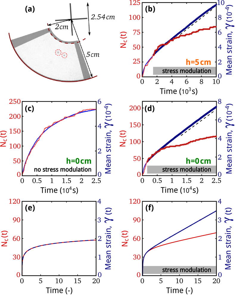
Figure 2: (a) Typical correlation map of the top surface. Two typical “hot spots” are visible. The shaded part is not used in the analysis. (b-d) Comparison of the mean strain, $\gamma(t)$ (blue) and the cumulative number of spots, $N_{c}(t)$ (red) as a function of time for three experiments performed at the same mean stress, $\sigma_{0}=1000Pa$ without (b) or with (c-d) stress modulation ($\delta=10Pa$, $f_{\sigma}=0.1Hz$). Experiments (c) and (d) are performed at $h=0\ cm$, experiment (b) at $h=5\ cm$. The grey strip shows when the modulation is on. (e)-(f) Mean strain, $\gamma(t)$ (blue) and cumulative fluidity, $N_{c}(t)$ (red) obtained by the numerical resolution of eqs. (4-5) taking into account the Couette geometry of the system, without (e) and with (f) stress modulation around the same mean stress. Parameters : $a=1$, $\sigma_{0}=0.8\sigma_{D}$, $f_{0}=1$, modulation: $\delta=0.005\sigma_{D}$ and $f_{\sigma}=0.2$.

Fig. 3a shows $N_{c}(t)$ normalized by $S/\sigma_{0}$ as a function the global plastic deformation for experiments performed at the same stress for either $h=0\ cm$ (green) or $h=5\ cm$ (orange). Without modulation (fine lines in Fig. 3.a), the proportionality between $N_{c}(t)$ and $\gamma(t)$ observed already in [5] is recovered, with a smaller slope in the case of $h=5\ cm$ (fine orange line) compared to the case $h=0\ cm$ (fine green line). When the stress modulation is turned on, we also obtain, after a transient regime, a proportional relationship between $N_{c}(t)$ and $\gamma(t)$ but with a smaller slope. This proportionnality shows that the macroscopic plastic deformation is the result of the accumulation of local plastic events. The coefficient of proportionality depends thus on the value of $h$ but also on the regimes (relaxation or rectified-regime). For the latter, the “hot-spots” production rate inducing similar plastic deformations when compared to the relaxation-regime values, is significantly smaller (Fig. 3a). The change of the slope is visible in both experiments at $h=0$ and $5\ cm$. Finally, two experiments with stress modulation for each depth are superimposed, showing the reproducibility of the measurements.

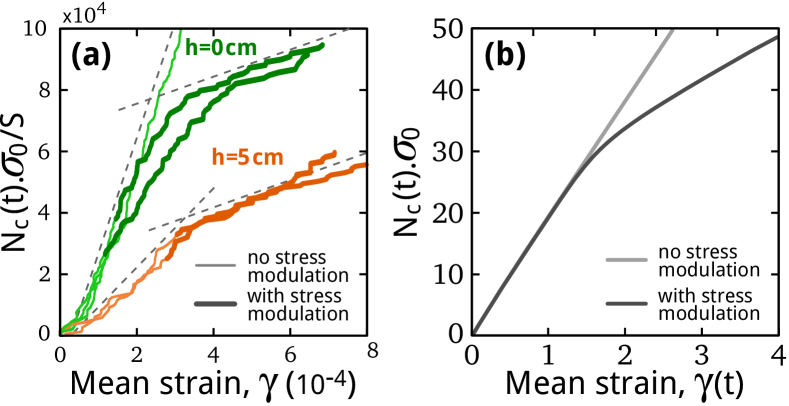
Figure 3: Normalized cumulative number of hot-spots as a function of the mean strain for 5 different experiments performed at $\sigma_{0}=1000Pa$. Green lines: $h=0cm$, orange lines: $h=5cm$. Fine line: no modulation, thick lines: with modulation. Dash lines are guide to the eye. (b) Corresponding graph obtained by numerical resolution of eq. (4-5) taking into account the geometry of the system. Same parameters as Fig 2.e-f.

4 Rheological model

The observed linear creep was interpreted in [13] as a secular drift, i.e. the accumulation of tiny effects over a very long time. The ingredients necessary for this sub-threshold fluidization by mechanical fluctuations to take place are the combination of shear rejuvenation and memory effect. Such ingredients are taken into account in the simplest mathematical way in a model put forwards by Derec et al. [11], to render the macroscopic phenomenology of aging complex fluids. This model was used successfully to interpret experimental strain relaxation curves and rectified creep in previous works [4, 20, 13]. A central parameter in this model is a fluidity variable $f$ representing the rate of visco-elastic relaxation for the shear stress $\sigma$ :

$$\dot{\sigma}=G\dot{\gamma}-f\sigma$$ (1)

$G$ is the shear elastic modulus. The rheological complexity stems from the dynamical equation undertaken by the fluidity variable. Many forms were suggested by Derec et al. [11], but in the context of granular creeping flow the experiment results point on a simple expression :

$$\dot{f}=-af^{2}+r\dot{\gamma}^{2}$$ (2)

where dimensionless parameters $a$ and $r$ represent respectively ageing and shear-induced rejuvenation processes. This model naturally induces a logarithmic relaxation under constant shear and also a dynamical threshold $\sigma_{D}=G\sqrt{a/r}$. In the context of granular matter this threshold value should be proportional to the confining pressure to get a Coulomb dynamical friction coefficient. Experiments [4] seems to indicate that under large shear, major reorganizations may occur in the packing and one should not consider anymore $a$ and $r$ as stress independent parameters. Recently, Pons et al. [13] have shown theoretically that the threshold of a visco-elastic fluid describes by this model will be destroyed by vanishingly small stress fluctuations around a bias by a secular effect. Consequently, below the threshold ($\sigma_{0}<\sigma_{D}$), an effective viscosity is expected of the form:

$$\eta=\frac{G\sigma_{D}}{\omega\delta}\sqrt{2\left(1-\frac{\sigma_{0}^{2}}{\sigma_{D}^{2}}\right)}.$$ (3)

In the following, we will consider the present model in its simple form ($a$ and $r$ constant) to see if at least qualitatively the salient experimental outcomes can be recovered.

The rheological equations (1) and (2) present rescaling parameters which are for stress $\sigma_{D}=G\sqrt{a/r}$, for deformation $\gamma_{0}=\sigma_{D}/G$, for fluidity $R_{\sigma}/\sigma_{D}$ and for time $\sigma_{D}/R_{\sigma}$. Then the dimensionless equations are as follows

$$\dot{\sigma}=\dot{\gamma}-f\sigma$$ (4)

$$\dot{f}=-a(f^{2}-\dot{\gamma}^{2})$$ (5)

Note that in this dimensionless representation the only remaining material parameter is $a$ and the only control parameters describing the stress are the dimensionless mean stress and amplitude: $\sigma_{0}/\sigma_{D}$ and $\delta/\sigma_{D}$. This system of equations can then be solved numerically to reproduce the experimental protocol. In presence of stress modulation, the resulting plastic deformation exhibits a transient logarithmic response followed by a linear regime (Fig. 2f). As we established before [13], this is qualitatively what is observed experimentally. The model allows thus to recover the general experimental behaviour as far as global deformation is concerned.

Several works have shown experimentally a direct relation between the rate of plastic events and the fluidity variable $f$ [5, 21]. However, it is not clear a priori that the mechanical driving would generate the same modes of plastic relaxation in the packing in the presence of the mechanical perturbations. And indeed, in fig. 3a, one can identify a systematic change of slope for the relation between the cumulated number of ”hot-spots” and the mean strain in the presence of stress modulation. This experimental fact leads to a central question on the relation between the rate of “hot spots” production and the fluidity parameter. This is the central object of the incoming discuccion.

5 Spatial response

Provided the assumption of a constant linear relationship between the rate of hot-spots production and the fluidity, the local and global distribution of hot-spot events can be computed. First, the radial heterogeneity of the stress field is taken into account in the model, i.e. $\sigma(r)=\sigma(R_{0})R_{0}^{2}/r^{2}$. However, here we do not account for the vertical heterogeneities as for example would be the case for experiments with the vane buried.

Eqs. (4) and (5) are then integrated numerically for each $r$ giving local values of the fluidity $f(r)$ and strain $\gamma(r)$. Because of the cylindrical geometry, the total rate of hot-spots occurrence is then expected to be proportional to $\int_{R_{0}}^{R}f(r)rdr$. The cumulated number of spot $N_{c}(t)$ can then be obtained numerically (within a multiplicative constant) by integrating this rate over time: $N_{c}(t)=\int_{0}^{t}\int_{R_{0}}^{R}f(\tau,r)rd\tau dr$. In parallel, $\gamma(r)$ is integrated over $r$ in order to obtain the rotation angle $\alpha(t)$ of the vane. Thus we can obtained numerically the mean strain $\gamma(t)=\alpha(t)R_{0}/(R-R_{0})$ corresponding to the one experimentally measured. Those two quantities are compared to the dimensionless time in Fig. 2e-f. In the case of Fig. 2e no stress modulation is considered and we recover the behaviour of the model when no spatial dependence is taken into account [4, 5]. In the case of Fig. 2f, stress modulation are imposed from $t=0$ and in this last case we observe a change of creep regime after a transient regime, in agreement with the experimental graphs of Fig. 2b and d. Finally, Fig. 3b shows the relationship between $N_{c}(t)$ and $\gamma(t)$ obtained numerically in each case. This relationship is the same as the one observed in experiments: the integral of the fluidity is proportional to the plastic deformation and for the rectified creep, a strong reduction of the slope is observed when the transient is terminated.

Therefore, the outcome of the simulations is qualitatively very similar to the experimental results. In particular, the change of slope in Fig. 3a is reproduced in the rheological model when the heterogeneity of the stress field due to the geometry is taken into account. Microscopically, this reduction originates from a difference in spatial distribution of “hot spots” for the two cases as we show numerically and experimentally in Fig. 4. Fig. 4a (resp. b) shows the radial evolution of the fluidity parameter without (resp. with) stress modulation at different time of the numerical integration. For the simple relaxation regime (logarithmic creep), the fluidity is quite homogeneous across the cell and thus rather independent of the local stress. The fluidity decreases uniformly with time, reflecting the decrease of the strain rate. On the contrary, for the rectified regime (Fig. 4b), the fluidity is quite different close or further away from the centre. It reaches rapidly a permanent regime with a high density value close to the centre while far from it, the density behaviour is close to the one observed without modulation.

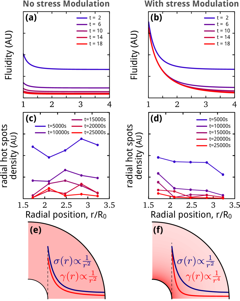
Figure 4: (a-b) Numerical resolution of eq. (4-5) taking into account the geometry of the system: evolution of the radial spatial fluidity over time whitout and with stress modulation, respectively. (c-d) Experimental results displaying the evolution of the radial hot spots density over time (experiments of Fig. 2c and d respectively). The vertical axis unit is arbitrary but identical for both experiments. (e) Schematic of the mechanical response in absence of modulation: the fluidity is spatially uniform in the cell (pink uniform background); the stress and the strain have the same spatial dependence. (f) Rectified case: the fluidity is non uniform and decreases as $\propto 1/r^{2}$.

The radial distribution of hot-spots production can also be obtained experimentally and and are shown in Fig. 4c (without modulations) and d (with modulations). The different curves correspond to the time evolution of the density. The density is calculated by averaging the number of “hot spots” over a time windows of $5000s$ and for a $5mm$ wide annulus. We first observe that this density decreases with time for both experiments. Then, although the data are quite noisy due to the small statistics, it seems that this radial density stays homogeneous for the simple relaxation (Fig. 4c) while the apparition of “hot spots” decreases more rapidly far from the center of the cell during the rectified creep (Fig. 4d), which qualitatively corroborates the outcome of the numerical measurements.

6 Discussion

To interpret this difference of behaviour in the radial spatial repartition of fluidity in the two regimes, we use the analytical results obtained from the perturbative analysis done in [13], but here, we explicitly take into account the spatial dependence of the stress. In absence of modulation, the fluidity is mostly governed by its initial value $f_{0}$ [4]:

$$f(r,t)=\frac{f_{0}}{1+af_{0}\left(1-\frac{\sigma_{0}^{2}(r)}{\sigma_{D}^{2}}\right)t}\approx\frac{f_{0}}{1+af_{0}t}$$ (6)

Consequently, when $\sigma_{0}\ll\sigma_{D}$, the non-rectified fluidity is independent of the radial position, a result recovered both in numerical solution (Fig. 4a) and in experiment (Fig. 4c). Yet, it uniformly slowly decreases with time. We thus obtain $\dot{\gamma}(r,t)=\frac{f(t)\sigma_{0}(r)}{G}\propto 1/r^{2}$. This case is schematically represented in Fig. 4e.

On the other hand, in the rectified case, as recalled in the description of the rheological model (eq. 3), the local stationary value $f^{*}(r)$ of the fluidity is for $\sigma_{0}\ll\sigma_{D}$ [13]:

$$f^{*}(r)=\frac{\omega\delta(R_{0})}{\sigma_{D}\sqrt{2}}\frac{R_{0}^{2}}{r^{2}},$$ (7)

If we suppose that a stationary solution is reached across the cell, we obtain for the local strain rate $\dot{\gamma}(r)=\frac{f^{*}(r)\sigma_{0}(r)}{G}\propto 1/r^{4}$. In this case, represented in Fig. 4f, the strain is highly localized in the vicinity of the blades.

Because of the strong decrease of the fluidity with $r$ in the rectified case, the total activity in the cell for a given mean strain across the cell is smaller in the case of Fig. 4f than of Fig. 4e. This is the origin of the decrease of the slope in Fig 3 in the rectified regime. Note that further refinement of the discussion taking into account that the stationary solution, in the rectified case, is not reached at large $r$ does not change the picture. The duration of the transients are nevertheless of major importance in such experiments and it can be problematic to conclude on the nature of the creep. Indeed, the time for the transient to reach the stationary solution $f^{*}$ is typically $1/f^{*}$ which diverges when the targeted fluidity decreases. Actually, the distinction between a rectified creep of very small $f^{*}$ and a logarithmic creep could be pointless experimentally. The time to reach the stationary solution may become increasingly long while environmental background noise, always presents in practice, may eventually hinder the latter.

7 Conclusion

In this report, we studied the creep response of a granular packing below the Coulomb fluidization threshold, both in the case of a logarithmic relaxation and for the mechanically rectified regime leading to a linear creep. In both cases, the global plastic deformation was monitored in parallel with the production rate of local plastic events. The experimental results were compared to the outcome of a simple visco-elastic model, solved numerically in the cylindrical geometry, which associates the local fluidity parameter to a rate of hot-spots production. Even though this model is quite simple, the salient experimental features were reproduced semi-quantitatively. First the effective linear relation between the cumulated number of hot-spots and the plastic deformation is recovered with a larger slope in the transient as compared to the rectified regime. Second, the qualitative features of the spatial distribution of hot spots are recovered in the model in both regimes: a weak radial dependence and an almost uniform decrease with time in the logarithmic creep case; and in the case of a linear creep, strong spatial dependence of the stationary solution close to the inner cylinder.

Interestingly, at this point, we do not need any non-local model to reproduce those generic experimental features. Heterogeneities of the stress field need to be taken into account to fully understand the data but not any spatial diffusion of the fluidity which is currently taken into account in more sophisticated fluidity models [6, 7, 8, 9]. However, it is important to note that this result does not necessarily exclude the generic presence of non-local terms in the rheological picture. It may simply mean that in the present experiments the non-local terms would not contribute significantly to the rheology. The experiments were performed at two different depths of the shearing vane, in the bulk and at the surface with an over-load inducing an equivalent confining ptressure. Hot-spots were observed in both configurations but the slope between the cumulated number of hot-spots and the plastic deformation differs. A further step to infirm or confirm that a local model is sufficient for the interpretation of all our data would be to test if this change of slope can be recovered when taking into account the full stress spatial distribution when the vane is buried or not. Indeed, the presence of hot-spots in the case when the vane is buried may be indicative of the spatial propagation of the plastic activity through the material bulk and thus of non-locality.

Finally, we must underline that most of the present results were obtained rather far from the dynamical threshold, where essentially, we could individualize the hot-spot apparition. Closer to the threshold and possibly due to spatial coupling and avalanching events, it would be interesting to see if quantitatively the simple local description still holds.

- [1] \NameWood D. M. \BookSoil Behaviour and Critical State Soil Mechanics \PublCambridge University Press, Cambridge \Year1990.
- [2] \NameNichol K., Zanin A., Bastien R., Wandersman E., van Hecke M. \REVIEWPhys. Rev. Lett.1042010078302.
- [3] \NameReddy A., Forterre Y., Pouliquen O. \REVIEWPhys. Rev. Lett.1062011108301.
- [4] \NameNguyen V. B., Darnige T., Bruand A., Clément E. \REVIEWPhys. Rev. Lett.1072011138303.
- [5] \NameAmon A., Nguyen V. B., Bruand A., Crassous J., Clément E. \REVIEWPhys. Rev. Lett.1082012135502.
- [6] \NameHenann D. L., Kamrin K. \REVIEWProc. Natl. Acad. Sci. USA11020136730.
- [7] \NameBouzid M., Trulsson M., Claudin P., Clément E., Andreotti B. \REVIEWPhys. Rev. Lett.1112013238301.
- [8] \NameHenann D. L., Kamrin K. \REVIEWPhys. Rev. Lett.1132014178001.
- [9] \NameM. Bouzid, A. Izzet, M. Trulsson, E. Clement, P. Claudin Andreotti B. \REVIEWEuropean Journal of Physics E382015125.
- [10] \NameSchmertmann J. H. \REVIEWJ. Geotech. Eng.11719911288.
- [11] \NameDerec C., Ajdari A., Lequeux F. \REVIEWEur. Phys. J. E42001355.
- [12] \NameLe Bouil A., Amon A., McNamara S., Crassous J. \REVIEWPhys. Rev. Lett.1122014246001.
- [13] \NamePons A., Amon A., Darnige T., Crassous J., Clément E \REVIEWPhys. Rev. E Rapid Com.922015020201(R).
- [14] \NameMøller P. C. F., Fall A., Bonn D. \REVIEWEPL87200938004.
- [15] \NameMarchal P., Smirani N., Choplin L. \REVIEWJournal of Rheology5320091.
- [16] \NameNegi A., Osuji C. \REVIEWEPL90201028003.
- [17] \NameSiebenbürger M., Ballauff M., Voigtmann T. \REVIEWPhys. Rev. Lett.1082012255701.
- [18] \NameErpelding M., Amon A., Crassous J. \REVIEWPhys. Rev. E782008046104.
- [19] \NameErpelding M., Amon A., Crassous J. \REVIEWEPL91201018002.
- [20] \NameEspíndola D., Galaz B., Melo F. \REVIEWPhys. Rev. Lett.1092012158301.
- [21] \NameJop P., Mansard V., Chaudhuri P., Bocquet L., Colin A. \REVIEWPhys. Rev. Lett.1082012148301.