Semilocal Density Functional Theory with correct surface asymptotics

Abstract

Semilocal Density Functional Theory is the most used computational method for electronic structure calculations in theoretical solid-state physics and quantum chemistry of large systems, providing good accuracy with a very attractive computational cost. Nevertheless, because of the non-locality of the exchange-correlation hole outside a metal surface, it was always considered inappropriate to describe the correct surface asymptotics. Here, we derive, within the semilocal Density Functional Theory formalism, an exact condition for the image-like surface asymptotics of both the exchange-correlation energy per particle and potential. We show that this condition can be easily incorporated into a practical computational tool, at the simple meta-generalized-gradient approximation level of theory. Using this tool, we also show that the Airy-gas model exhibits asymptotic properties that are closely related to the ones at metal surfaces. This result highlights the relevance of the linear effective potential model to the metal surface asymptotics.

I Introduction

The exact form of the potential felt by an electron leaving from or approaching a metal surface is of great importance for a variety of physical phenomena, including the interpretation of image states Garcia et al. (1985), modeling quantum-transport Datta (2005), low-energy electron diffraction (LEED) Rundgren and Malmström (1977), scanning tunneling microscopy Binnig et al. (1985); Pitarke et al. (1990), and inverse or two-photon photoemission spectroscopy Harris et al. (1997); Fauster and Steinmann (1995). The asymptotic form of this image potential is $-1/(4(z-z_{0}))$, with $z$ being the distance from the surface, and $z_{0}$ representing the position of the so-called image planeLang and Kohn (1973), and should be reproduced by any computational method aiming at an accurate description of the surface physics.

Within Kohn-Sham (KS) density-functional theory (DFT) Kohn (1999); Kohn and Sham (1965), which is the most used computational method for electronic structure calculations in theoretical solid-state physics, the shape of the image potential is dictated by the properties of the effective Kohn-Sham (KS) potential. This depends on the employed approximation for the exchange-correlation (XC) functional $E_{xc}[\rho]$, which gives the XC potential via the relation

$$v_{xc}({\bf r})={\delta E_{xc}[\rho]\over\delta\rho({\bf r})},$$ (1)

where $\rho$ is the electron density. It has been shown that the exact $v_{xc}$ asymptotically approaches the image potential Lang and Kohn (1973); Gunnarsson et al. (1979); Eguiluz and Hanke (1989); Eguiluz et al. (1992); White et al. (1998), despite a different result has been obtained within the plasmon-pole approximationQian and Sahni (2005).

The popular local density approximation (LDA) Kohn and Sham (1965) and the generalized-gradient approximation (GGA), however, fail in this task Hoeft et al. (2001) showing either a too fast decay (e.g. exponential), or an inaccurate description of the surface energetics (as for the Becke exchange Becke (1988)). Ad-hoc modifications of the LDA XC potential Serena et al. (1986); Chulkov et al. (1999) have then been proposed to improve the asymptotic behavior of the XC potential, but such methods are not functional derivatives of any energy functional. Alternatively, non-local methods outside the KS framework Gunnarsson et al. (1979); Gunnarsson and Jones (1980); Ossicini et al. (1986); García-González et al. (2000); Eguiluz et al. (1992); White et al. (1998) are employed.

An accurate KS-DFT method with the correct surface asymptotics would be desirable for many reasons, including the local nature and the computational efficiency. However, a good functional shall yield not only the correct asymptotic XC potential, but also accurate energies. Thus, it is necessary to be defined by a realistic energy per particle $\varepsilon_{xc}({\bf r})$. The latter is not a uniquely defined physical quantity, but an exact reference for it is the the conventional energy per particle, which is associated with the interaction of an electron at ${\bf r}$ with the coupling-constant-averaged charge of its XC hole Harris and Griffin (1975); Langreth and Perdew (1977); Gunnarsson and Lundqvist (1976). The exact (conventional) $\varepsilon_{xc}({\bf r})$ at metal surfaces decays as $-1/(4(z-z_{0}))$, i.e. as the image potential Gunnarsson et al. (1979); Constantin and Pitarke (2011).

We recall that the exact exchange energy per particle decreases as $\epsilon_{x}(z\rightarrow\infty)\rightarrow-A(\beta)/z$ where $A(\beta)=(\pi+2\beta\ln(\beta))/(2\pi(1+\beta^{2}))$, $\beta=\sqrt{\epsilon_{F}/W}$, $\epsilon_{F}=k_{F}^{2}/2$ being the Fermi energy (and $k_{F}$ the Fermi wavevector), and $W$ the work function Horowitz et al. (2009); Qian (2012). On the other hand, the exact exchange potential behaves as $v_{x}(z\rightarrow\infty)\rightarrow\ln(\beta k_{F}z)/(2\pi\beta z)$Horowitz et al. (2010). Note that these behaviors are related to semi-infinite surfaces; for finite jellium slabs we have that, as in molecules, $\epsilon_{x}(z\rightarrow\infty)=-1/(2z)$ Horowitz et al. (2009) and $v_{x}(z\rightarrow\infty)=-1/(z)$Horowitz et al. (2006, 2008); Ye (2015); Engel (2014a, b).

The simultaneous description of surface asymptotic and energy properties is anyway an ambitious objective, which is in fact not achievable at the GGA level Engel et al. (1992); van Leeuwen and Baerends (1994); Armiento and Kümmel (2013); Della Sala et al. (2015). In this article, we show that the issue can be instead solved at the meta-GGA level of theory, employing an exact condition which yields the correct image-like asymptotic behavior of both $\varepsilon_{xc}$ and $v_{xc}$ at metal surfaces. This condition can be easily implemented in any meta-GGA functional, keeping its original accuracy for ground-state properties not related to surface asymptotics. Hence, an accurate KS-DFT method with correct metal-surface asymptotic can be obtained for application in many surface science problems.

II Exact condition for asymptotic properties

To start, we consider the simplest (and most used) model for a metal surface: the semi-infinite jellium surface. This model system is very important in surface science and solid-state physics, containing the physics of simple metal surfaces Lang and Kohn (1970, 1971, 1973).

The KS single-particle orbitals have the form

$$\Psi_{k_{z},\mathbf{k}_{||}}(\mathbf{r})=\frac{1}{\sqrt{S}\sqrt{L}}e^{i\mathbf{k}_{||}\mathbf{r}_{||}}\phi_{k_{z}}(z)\ ,$$ (2)

where $\mathbf{k}_{||}$ and $\mathbf{r}_{||}$ are the two-dimensional wave-vector and position vector in the plane $xy$ of the surface, $k_{z}$ and $z$ are the corresponding components in the direction perpendicular to the surface, $S$ and $L$ are the normalization area and length, and $\phi_{k_{z}}(z)$ are the eigenfunctions of a one-dimensional KS Hamiltonian (for details see Appendix A).

In the vacuum region, far away from the surface ($z\to\infty$), the single-particle orbitals $\phi_{k_{z}}(z)$ behave as Horowitz et al. (2009):

$$\phi_{k_{z}}(z\rightarrow\infty)\rightarrow\phi_{k_{F}}(z\rightarrow\infty)e^{-\beta z(k_{F}-k_{z})},$$ (3)

where

$$\phi_{k_{F}}(z\rightarrow\infty)\sim e^{-z\sqrt{2W}}(2z\sqrt{2W})^{\alpha_{KS}/\sqrt{2W}},$$ (4)

$\alpha_{KS}>0$.

Now, we consider a meta-GGA XC energy per particle of the form

$$\epsilon_{xc}^{MGGA}=\epsilon_{x}^{LDA}\frac{1}{\eta}\frac{8\pi}{3\sqrt{5}}\frac{\sqrt{\alpha}}{\sqrt{\ln(\alpha)}}\ ,$$ (5)

where $\eta$ is a parameter to be fixed later, $\alpha(\mathbf{r})=\left[\tau(\mathbf{r})-\tau^{W}(\mathbf{r}))/\tau^{TF}(\mathbf{r})\right]$ is the well-known meta-GGA ingredient that measures the non-locality of the kinetic-energy density Della Sala et al. (2015), with $\tau$, $\tau^{W}$, and $\tau^{TF}$ being the positive-defined exact KS, von Weizsäcker, and Thomas-Fermi kinetic-energy densities, respectively. We recall that $1/\left[1+\alpha(\mathbf{r})^{2}\right]$ is the electron localization function, often used in the characterization of chemical bonds Silvi and Savin (1994). Eq. (5) yields the following asymptotic behaviors (see the Appendix B for details):

$$\epsilon_{xc}^{MGGA}(z\rightarrow\infty) \rightarrow -\frac{1}{\eta}\frac{1}{z}+\mathcal{O}(z^{-2}),$$ (6)

$$v_{xc}^{MGGA}(z\rightarrow\infty) \rightarrow -\frac{3}{2\eta}\frac{1}{z}+\mathcal{O}(z^{-2})\ .$$ (7)

Here, the KS potential has been obtained in the generalized KS framework using the formula Arbuznikov et al. (2002)

$$v_{xc}(\mathbf{r})\Psi_{i}(\mathbf{r}) = [\frac{\partial(\rho\epsilon_{xc})}{\partial\rho}-\nabla\frac{\partial(\rho\epsilon_{xc})}{\partial\nabla\rho}]\Psi_{i}-\frac{1}{2}\nabla(\frac{\partial(\rho\epsilon_{xc})}{\partial\tau})\nabla\Psi_{i}$$ (8)

$$-\frac{1}{2}\frac{\partial(\rho\epsilon_{xc})}{\partial\tau}\nabla^{2}\Psi_{i}\ .$$

Equations. (6) and (7) show that, in contrast to previously developed XC functionals, both $v_{xc}$ and $\epsilon_{xc}$ are proportional to the exact ones: if $\eta=\eta_{1}=4$ ($\eta=\eta_{2}=6$) then the exact energy-density (potential) is obtained. Unfortunately, $\eta_{1}\neq\eta_{2}$. Nevertheless, for both values Eq. (5) yields an asymptotic behavior qualitatively and quantitatively significantly beyond the current state-of-the-art. We also remark that Eq. (5) is solely based on the properties of the reduced kinetic ingredient $\alpha$. However, at the meta-GGA level of theory, other ingredients are also available (e.g. the gradient and the Laplacian of the density) so that the exact asymptotic description of both $\epsilon_{xc}$ and $v_{xc}$ might be achieved.

III Practical computational tool

As a first practical example, we consider the case $\eta=\eta_{1}$ and incorporate the condition of Eq. (5) into the popular TPSS meta-GGA functional Tao et al. (2003), using an approach similar to that of Ref. Constantin et al., 2015. The resulting XC functional will be termed surface-asymptotics (SA) TPSS. This functional is obtained by simply changing, in the TPSS exchange formula, the parameter $\kappa$ (which determines the asymptotic behavior of the functional) from its original value of 0.804 to

$$\kappa=\frac{2\pi}{3\sqrt{5}}\frac{\sqrt{\alpha+1}}{\sqrt{a+\ln(\alpha+b)}}\ .$$ (9)

The correlation is left unchanged. (Note that the TPSS correlation decays exponentially, and thus our XC condition is incorporated in the TPSS exchange functional. This is a common procedure for semilocal functionals, which are based on a strong error cancellation between the exchange and correlation parts.) In Eq. (9), the parameters $a=2.413$ and $b=0.348$ have been fixed by imposing the constraints: $\kappa=0.804$ for $\alpha=1$ and $\alpha=0$; whereas, when degenerate orbitals contribute to the tail of the density ($\alpha\rightarrow\infty$), $\kappa\rightarrow\frac{2\pi}{3\sqrt{5}}\frac{\sqrt{\alpha}}{\sqrt{\ln(\alpha)}}$ (i.e. Eq. (5)). These conditions assure that (i) all the exact constraints satisfied by the original TPSS exchange functional are preserved and (ii) the new functional yields the correct image-like asymptotics. The SA-TPSS functional does not recover locally the Lieb-Oxford bound Constantin et al. (2015), as TPSS does, but it satisfies the global Lieb-Oxford bound for all known physical systems (e.g. for atoms, molecules, solids and surfaces $E_{xc}^{SA-TPSS}\approx E_{xc}^{TPSS}$). Moreover, it fulfills locally the simplified version of the Lewin-Lieb bound (see Eq. (22) of Ref. Feinblum et al. (2014)).

Figure 1: TPSS and SA-TPSS exchange enhancement factors versus $\alpha$, for three values of the reduced gradient $s$.

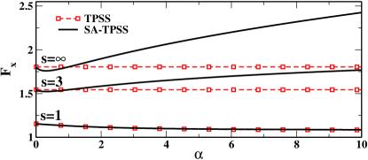
In Fig. 1, we show the TPSS and SA-TPSS exchange enhancement factors versus $\alpha$ for several values of the reduced gradient $s=|\nabla\rho|/(2(3\pi^{2})^{1/3}\rho^{4/3})$). When $s$ is small, TPSS and SA-TPSS coincide for all values of $\alpha$. As $s$ increases, TPSS and SA-TPSS start to differ, especially at large values of $\alpha$, as expected.

Figure 2: $z\epsilon_{xc}(z)$ (upper panel) and $zv_{xc}(z)$ (lower panel) versus the reduced distance $z/\lambda_{F}$ ($\lambda_{F}$ is the Fermi wavelength), for a jellium surface with electron-density parameter $r_{s}=2$ and $r_{s}=4$. The surface is located at $z=0$. Note that SA-TPSS gives $z\epsilon_{xc}=-1/4$ and $zv_{xc}=-3/8$ far outside the surface.

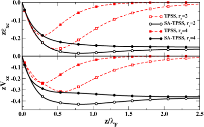
In Fig. 2, fully self-consistent KS-LDA orbitals were used to obtain $z\epsilon_{xc}(z)$ (upper panel) and $zv_{xc}(z)$ (lower panel) as a function of the scaled distance $z$ for jellium surfaces with the electron-density parameters $r_{s}=2$ and $r_{s}=4$. The TPSS functional yields a wrong (exponential) asymptotic behavior for both quantities. Instead, the SA-TPSS functional gives the following asymptotic behaviors: $\epsilon_{xc}(z)\rightarrow-0.25/z$ and $v_{xc}(z)\rightarrow-0.375/z$. Thus, Fig. 2 provides a numerical proof of the validity of Eq. (5), as well as a validation of the simple construction used to obtain the SA-TPSS functional.

Table 1: Jellium surface energies (in erg/cm²), as obtained by using the functionals TPPS and SA-TPSS for various values of the electron-density parameter $r_{s}$. Diffusion Monte Carlo (DMC) calculations Wood et al. (2007) are given as a reference. The results of the popular LDA Kohn and Sham (1965); Perdew and Wang (1992) and PBE Perdew et al. (1996) functionals, are also shown for comparison.

$r_{s}$	TPSS	SA-TPSS	LDA	PBE	Ref.
2	3380	3368	3354	3265	3392 $\pm$ 50
3	772	767	764	741	768 $\pm$ 10
4	266	263	261	252	261 $\pm$ 8
6	55.5	54.5	53	52	53 $\pm$ …

Table 2: Mean absolute errors (in kcal/mol for energetical tests and in mÅ  for the bond length test) of several molecular properties Constantin et al. (2013); Fabiano et al. (2013).

Test	TPSS	SA-TPSS	LDA	PBE
atomization energies (W4 test)	4.7	4.8	44.0	10.7
reaction energies (OMRE test)	8.0	7.9	21.0	6.7
ionization potentials (IP13 test)	3.1	3.1	4.9	3.0
bond lengths (MGBL19 test)	6.9	7.0	10.0	9.3
dipole interactions (DI6 test)	0.6	0.4	2.7	0.4
hydrogen bonds (HB6 test)	0.6	0.4	4.5	0.4

In Tables 1 and 2 we report the TPSS and SA-TPSS results for surface energies and various molecular tests, respectively. By construction, whenever the surface asymptotics plays a negligible role (e.g., covalent interactions in molecules: W4, OMRE, IP13, MGBL19) both functionals yield very similar results. In the case of jellium surface energies and non-covalent interactions (DI6, HB6), however, SA-TPSS improves over the standard TPSS.

Finally, we have to stress that the SA-TPSS meta-GGA gives only the correct asymptotic decay of the XC energy per particle and potential at metal surfaces, but it can not provide the exact behavior for the exchange and correlation components, separately. This is a difficult task, that in our opinion, a simple semilocal functional can not obey.

IV Airy gas asymptotic properties

As an additional example of the use of Eq. (5) and of the SA-TPSS functional, we consider the Airy gas Kohn and Mattsson (1998); Armiento and Mattsson (2005), which is the simplest possible model for an edge electron gas (for details see Appendix A). This model system plays an important role in DFT Armiento and Mattsson (2005); Vitos et al. (2000a); Constantin and Ruzsinszky (2009), as it incorporates the correct physics of a semi-infinite metal surface and is simple enough to allow for analytical calculations. To our knowledge, the exact asymptotic behavior of the XC energy per particle and of KS XC potential of the Airy gas are unknown. Nevertheless, we can use the SA-TPSS functional to obtain some information about them.

The Airy-gas electron density and positive-defined kinetic-energy density are Kohn and Mattsson (1998); Armiento and Mattsson (2005); Vitos et al. (2000a, b)

$$\rho(z) = \frac{1}{3\pi}[z^{2}\rm{Ai}^{2}(z)-z\rm{Ai^{\prime}}^{2}(z)-\rm{Ai}(z)\rm{Ai^{\prime}}(z)/2],$$ (10)

$$\tau = -\frac{3}{10}z\rho(z)+\frac{1}{5}\rho^{\prime\prime}(z)\ ,$$ (11)

where $z$ is the scaled distance and ${\rm Ai}(z)$ is the Airy function.

Figure 3: The Airy-gas semilocal ingredients ($s$, $q$, and $\alpha$), as a function of the scaled distance $z$. The Airy bulk is at $z\leq 0$. The exponential decay of the electron density occurs at $z\geq 0$.

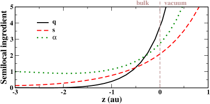
In Fig. 3, we show the Airy-gas semilocal ingredient $s$, the reduced Laplacian $q=\nabla^{2}\rho/[4(3\pi^{2})^{2/3}\rho^{5/3}]$, and $\alpha$. In the bulk ($z\rightarrow-\infty$), both $s$ and $q$ are small, while $\alpha\rightarrow 1$ (showing that the Thomas-Fermi theory becomes exact). In the vacuum, all semilocal ingredients diverge (as in the case of the jellium surface).

In the limit $z\to\infty$, the Airy-gas electron density and kinetic-energy density are

$$\rho(z\rightarrow\infty) \rightarrow \frac{1}{32}\,{\frac{{{\rm e}^{-4/3\,{z}^{3/2}}}}{{\pi}^{2}z^{3/2}}}-{\frac{35}{768}}\,{\frac{{{\rm e}^{-4/3\,{z}^{3/2}}}}{{\pi}^{2}{z}^{3}}}+\ldots\,$$

$$\tau(z\rightarrow\infty) \rightarrow {\frac{1}{64}}\,{\frac{{{\rm e}^{-4/3\,{z}^{3/2}}}}{\sqrt{z}{\pi}^{2}}}+{\frac{13}{1536}}\,{\frac{{{\rm e}^{-4/3\,{z}^{3/2}}}}{{\pi}^{2}{z}^{2}}}+\ldots\ .$$ (12)

The SA-TPSS XC functional gives the following analytical expressions:

$$\epsilon_{xc}^{SA-TPSS}(z\rightarrow\infty) \rightarrow -\sqrt{3}/(8z)\approx-0.217/z,$$

$$v^{SA-TPSS}_{xc}(z\rightarrow\infty) \rightarrow -3\sqrt{3}/(16z)\approx-0.325/z.$$ (13)

This result is interesting, since it suggests that, for the Airy gas, both $\epsilon_{xc}$ and $v_{xc}$ decay as $-1/z$, as in the case of the jellium surface. Furthermore, because the coefficients (0.217 and 0.325) are close to, but smaller than, the ones for the jellium surface (0.25 and 0.375), we can conclude that at a metal surface the main contribution to the asymptotics comes from the region near the surface, where the effective potential is linear and well described by the Airy-gas model. We note that such a result cannot be obtained without the proper inclusion of exact surface conditions into the functional. This is shown in Fig. 4 where we plot, for several functionals, $z\epsilon_{xc}(z)$ (upper panel) and $zv_{xc}(z)$ (lower panel), versus the scaled distance $z$, in the vacuum region of the Airy gas.

Figure 4: The Airy-gas $z\epsilon_{xc}(z)$ (upper panel) and $zv_{xc}(z)$ (lower panel), as a function of the scaled distance $z$.

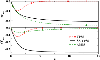
The TPSS functional shows a rather unphysical exponential decay for both $\varepsilon_{xc}$ and $v_{xc}$. On the other hand, the AM05 functional Armiento and Mattsson (2005), whose energy density is fitted to the Airy gas, is close to our SA-TPSS functional for $\epsilon_{xc}$ but displays a decay that is too fast for $v_{xc}$. This latter feature represents a manifestation of the impossibility, at the GGA level, to describe correctly both $\epsilon_{xc}$ and $v_{xc}$, which can only be overcome at the meta-GGA level Della Sala et al. (2015).

The exchange-only asymptotic behaviors ($\epsilon_{x}$ and $v_{x}$) at metal surfaces, are depending on the bulk and surface parameters ($k_{F}$ and $W$) Horowitz et al. (2009, 2010); Qian (2012), and thus they are created by bulk- and surface-electrons. When correlation is included, screening effects dump the bulk contribution, such that the asymptotic properties of $\epsilon_{xc}$ and $v_{xc}$ are mainly created by a density-independent XC effect of the surface region, as proved by the SA-TPSS result for the Airy gas. Thus, the Airy gas model system can be efficiently used in modelling various phenomena outside metal surfaces, even being an alternative to the ad-hoc LDA XC potential modifications Serena et al. (1986); Chulkov et al. (1999).

V Conclusions

In conclusion, we have derived an exact meta-GGA condition for the correct image-like surface asymptotics of the XC energy per particle $\varepsilon_{xc}$ and the KS XC potential $v_{xc}$. Our formula [Eq. (5)] depends only on the semilocal ingredient $\alpha$ and takes advantage of the non-locality of the kinetic energy density beyond the von Weizsäcker term Della Sala et al. (2015). The existence of this exact condition represents an important contribution in the framework of DFT, as it shows that surface asymptotics can be described by semilocal meta-GGA functionals. On the contrary, no GGA can be constructed that is able to describe correctly the asymptotics of both $\varepsilon_{xc}$ and $v_{xc}$. In fact, there is, to our knowledge, no GGA functional that yields a realistic KS XC potential at metal surfaces.

We have demonstrated that our exact condition can be easily implemented in any meta-GGA functional, keeping its original accuracy for standard ground-state properties and providing, at the same time, a correct description of the surface asymptotics. We have constructed the SA-TPSS functional, which we have shown to perform as the TPSS for covalent chemistry and to improve over it for non-covalent interactions and surface-related problems. This new functional can thus be a promising tool for the investigation of surface-sensitive electronic-structure calculations, such as molecule/molecular complex-surface, cluster-surface, and surface-surface interactions.

We thank TURBOMOLE GmbH for providing the TURBOMOLE program package.

APPENDIX A

In case of semi-infinite jellium surfaces, the one-particle eigenfunctions $\phi_{k_{z}}(z)$ have a continuous energy spectrum $\epsilon_{k_{z}}=V_{KS}(\infty)+k_{z}^{2}/2$, and are solutions of the one-dimensional KS equation

$$(-\frac{\partial^{2}}{2\partial z^{2}}+V_{KS}(z)-\epsilon_{k_{z}})\phi_{k_{z}}(z)=0.$$ (A-1)

Here $V_{KS}(z)=V_{H}(z)+V_{xc}(z)$ is the sum of the total classical electrostatic potential (which incorporates the positive background), and the XC potential.

In case of the Airy gas, the effective potential has the linear form

$$v_{eff}(Z)=\left\{\begin{array}[]{lr}-FZ&\;\rm{when}\;\;\;-\infty<Z<L\\ +\infty&\;\rm{when}\;\;\;Z\geq L,\end{array}\right.$$ (A-2)

with $F>0$ being the slope of the effective potential Kohn and Mattsson (1998). Thus, the one-particle normalized eigenfunctions $\phi_{j}(Z)$ satisfy the one-dimensional equation

$$(-\frac{\partial^{2}}{2\partial Z^{2}}-FZ-\epsilon_{j})\phi_{j}(Z)=0,$$

$$\phi_{j}(\infty)=\phi_{j}(L)=0,$$ (A-3)

being proportional to the Airy function. Here $Z$ is the distance perpendicular to the surface. It is convenient to consider the scaled distance $z=Z(2F)^{1/3}$ Kohn and Mattsson (1998), as used in the Section IV.

APPENDIX B

The electron density and kinetic energy density of a jellim surface are

$$\rho(z) = \frac{1}{4\pi^{2}}\int_{-k_{F}}^{k_{F}}dk_{z}\;(k_{F}^{2}-k_{z}^{2})|\phi_{k_{z}}(z)|^{2},$$ (B-1)

$$\tau(z) = \int_{-k_{F}}^{k_{F}}dk_{z}\;[\frac{1}{8\pi^{2}}|\frac{\partial\phi_{k_{z}}(z)}{\partial z}|^{2}(k_{F}^{2}-k_{z}^{2})+$$ (B-2)

$$\frac{1}{16\pi^{2}}|\phi_{k_{z}}(z)|^{2}(k_{F}^{2}-k_{z}^{2})^{2}]\ ,$$

with $k_{F}$ being the magnitude of the bulk Fermi wave-vector.

Using Eqs. (3) and (4) we obtain, when $z\rightarrow\infty$, the following expressions

$$\rho\rightarrow\left(1/4\,{\frac{{N}^{2}W}{{\it k_{F}}\,{\pi}^{2}{z}^{2}}}-1/8\,{\frac{{N}^{2}\sqrt{2}{W}^{3/2}}{{{\it k_{F}}}^{3}{z}^{3}{\pi}^{2}}}\right)e^{-2z\sqrt{2W}}z^{2\alpha_{KS}}$$ (B-3)

$$\tau\rightarrow 1/4\,{\frac{{N}^{2}{W}^{2}}{{\it k_{F}}\,{\pi}^{2}{z}^{2}e^{2z\sqrt{2W}}z^{-2\alpha_{KS}}}}+1/32\,{\frac{\left(-8\,{{\it k_{F}}}^{4}\sqrt{W}{\it\alpha_{KS}}-4\,{{\it k_{F}}}^{2}{W}^{3/2}+12\,{{\it k_{F}}}^{4}\sqrt{W}\right){N}^{2}W\,\sqrt{2}}{{{\it k_{F}}}^{5}{\pi}^{2}{z}^{3}e^{2z\sqrt{2W}}z^{-2\alpha_{KS}}}}+$$

$$1/32\,{\frac{\left(-12\,{{\it k_{F}}}^{2}W\,\sqrt{2}+3\,\sqrt{2}{{\it k_{F}}}^{4}+4\,{{\it k_{F}}}^{2}W\,\sqrt{2}{\it\alpha_{KS}}-4\,\sqrt{2}{{\it k_{F}}}^{4}{\it\alpha_{KS}}+2\,\sqrt{2}{{\it k_{F}}}^{4}{{\it\alpha_{KS}}}^{2}\right){N}^{2}W\,\sqrt{2}}{{{\it k_{F}}}^{5}{\pi}^{2}{z}^{4}e^{2z\sqrt{2W}}z^{-2\alpha_{KS}}}}+$$

$$1/32\,{\frac{\left(6\,{{\it k_{F}}}^{2}\sqrt{W}{\it\alpha_{KS}}+6\,{W}^{3/2}-2\,{{\it k_{F}}}^{2}\sqrt{W}{{\it\alpha_{KS}}}^{2}-6\,{{\it k_{F}}}^{2}\sqrt{W}\right){N}^{2}W\,\sqrt{2}}{{{\it k_{F}}}^{5}{\pi}^{2}{z}^{5}e^{2z\sqrt{2W}}z^{-2\alpha_{KS}}}}.$$ (B-4)

Then,

$$\alpha\rightarrow-\,{\frac{\left(-60\,\sqrt[3]{3}\sqrt[6]{2}{{\it k_{F}}}^{2}z\,\sqrt{W}+40\,\sqrt[3]{3}{2}^{2/3}W-15\,\sqrt[3]{3}{2}^{2/3}{{\it k_{F}}}^{2}\right){{\rm e}^{4/3\,z\,\sqrt{2}\sqrt{W}}}{z}^{-4/3\,{\it\alpha_{KS}}-2/3}{2}^{2/3}}{54{W}^{2/3}{N}^{4/3}{{\it k_{F}}}^{4/3}}},$$ (B-5)

and

$$F_{xc}\rightarrow\frac{4}{9\eta}{\frac{\left(\pi\,{2}^{2/3}{3}^{2/3}\sqrt[3]{{\it k_{F}}}+9\,O\left({z}^{-4/3}\right){N}^{2/3}\sqrt[3]{W}\sqrt[3]{z}\right){{\rm e}^{2/3\,z\,\sqrt{2}\sqrt{W}}}{z}^{-2/3\,{\it\alpha_{KS}}-1/3}}{{N}^{2/3}\sqrt[3]{W}}},$$ (B-6)

where $N$ is a normalization constant, $W$ is the work function, and $k_{F}$ is the bulk Fermi wave-vector. Here $F_{xc}=\epsilon_{xc}^{MGGA}/\epsilon_{x}^{LDA}$ is the enhancement factor corresponding to the energy density of Eq. (5).

References

- Garcia et al. (1985) N. Garcia, B. Reihl, K. H. Frank, and A. R. Williams, Phys. Rev. Lett. 54, 591 (1985), URL http://link.aps.org/doi/10.1103/PhysRevLett.54.591.
- Datta (2005) S. Datta, Quantum transport: atom to transistor (Cambridge University Press, 2005).
- Rundgren and Malmström (1977) J. Rundgren and G. Malmström, Phys. Rev. Lett. 38, 836 (1977).
- Binnig et al. (1985) G. Binnig, K. H. Frank, H. Fuchs, N. Garcia, B. Reihl, H. Rohrer, F. Salvan, and A. R. Williams, Phys. Rev. Lett. 55, 991 (1985).
- Pitarke et al. (1990) J. Pitarke, F. Flores, and P. Echenique, Surf. Sci. 234, 1 (1990), ISSN 0039-6028.
- Harris et al. (1997) C. B. Harris, N.-H. Ge, R. L. L. Jr., J. D. McNeill, and C. M. Wong, Ann. Rev. Phys. Chem. 48, 711 (1997).
- Fauster and Steinmann (1995) T. Fauster and W. Steinmann, in Electromagnetic Waves: Recent Development in Research, Vol. 2, edited by P. Halevi (Elsevier, Amsterdam, 1995), p. 350.
- Lang and Kohn (1973) N. Lang and W. Kohn, Phys. Rev. B 7, 3541 (1973).
- Kohn (1999) W. Kohn, Rev. Mod. Phys. 71, 1253 (1999).
- Kohn and Sham (1965) W. Kohn and L. J. Sham, Phys. Rev. 140, A1133 (1965).
- Gunnarsson et al. (1979) O. Gunnarsson, M. Jonson, and B. I. Lundqvist, Phys. Rev. B 20, 3136 (1979), URL http://link.aps.org/doi/10.1103/PhysRevB.20.3136.
- Eguiluz and Hanke (1989) A. G. Eguiluz and W. Hanke, Phys. Rev. B 39, 10433 (1989).
- Eguiluz et al. (1992) A. G. Eguiluz, M. Heinrichsmeier, A. Fleszar, and W. Hanke, Phys. Rev. Lett. 68, 1359 (1992).
- White et al. (1998) I. D. White, R. W. Godby, M. M. Rieger, and R. J. Needs, Phys. Rev. Lett. 80, 4265 (1998).
- Qian and Sahni (2005) Z. Qian and V. Sahni, Int. J. Quantum Chem. 104, 929 (2005).
- Hoeft et al. (2001) J.-T. Hoeft, M. Kittel, M. Polcik, S. Bao, R. L. Toomes, J.-H. Kang, D. P. Woodruff, M. Pascal, and C. L. A. Lamont, Phys. Rev. Lett. 87, 086101 (2001).
- Becke (1988) A. D. Becke, Phys. Rev. A 38, 3098 (1988).
- Serena et al. (1986) P. A. Serena, J. M. Soler, and N. García, Phys. Rev. B 34, 6767 (1986), URL http://link.aps.org/doi/10.1103/PhysRevB.34.6767.
- Chulkov et al. (1999) E. Chulkov, V. Silkin, and P. Echenique, Surface Science 437, 330 (1999), ISSN 0039-6028.
- Gunnarsson and Jones (1980) O. Gunnarsson and R. O. Jones, Physica Scripta 21, 394 (1980), URL http://iopscience.iop.org/1402-4896/21/3-4/027.
- Ossicini et al. (1986) S. Ossicini, C. M. Bertoni, and P. Gies, Europhy. Lett. 1, 661 (1986).
- García-González et al. (2000) P. García-González, J. E. Alvarellos, E. Chacón, and P. Tarazona, Phys. Rev. B 62, 16063 (2000).
- Harris and Griffin (1975) J. Harris and A. Griffin, Phys. Rev. B 11, 3669 (1975).
- Langreth and Perdew (1977) D. C. Langreth and J. P. Perdew, Phys. Rev. B 15, 2884 (1977).
- Gunnarsson and Lundqvist (1976) O. Gunnarsson and B. I. Lundqvist, Phys. Rev. B 13, 4274 (1976).
- Constantin and Pitarke (2011) L. A. Constantin and J. M. Pitarke, Phys. Rev. B 83, 075116 (2011).
- Horowitz et al. (2009) C. M. Horowitz, L. A. Constantin, C. R. Proetto, and J. M. Pitarke, Phys. Rev. B 80, 235101 (2009).
- Qian (2012) Z. Qian, Phys. Rev. B 85, 115124 (2012).
- Horowitz et al. (2010) C. M. Horowitz, C. R. Proetto, and J. M. Pitarke, Phys. Rev. B 81, 121106 (2010).
- Horowitz et al. (2006) C. M. Horowitz, C. R. Proetto, and S. Rigamonti, Phys. Rev. Lett. 97, 026802 (2006), URL http://link.aps.org/doi/10.1103/PhysRevLett.97.026802.
- Horowitz et al. (2008) C. M. Horowitz, C. R. Proetto, and J. M. Pitarke, Phys. Rev. B 78, 085126 (2008), URL http://link.aps.org/doi/10.1103/PhysRevB.78.085126.
- Ye (2015) L.-H. Ye, Phys. Rev. B 92, 115132 (2015).
- Engel (2014a) E. Engel, J. Chem. Phys. 140, 18A505 (2014a).
- Engel (2014b) E. Engel, Phys. Rev. B 89, 245105 (2014b).
- Engel et al. (1992) E. Engel, J. Chevary, L. Macdonald, and S. Vosko, Z. Phys. D 23, 7 (1992), ISSN 0178-7683.
- van Leeuwen and Baerends (1994) R. van Leeuwen and E. J. Baerends, Phys. Rev. A 49, 2421 (1994).
- Armiento and Kümmel (2013) R. Armiento and S. Kümmel, Phys. Rev. Lett. 111, 036402 (2013).
- Della Sala et al. (2015) F. Della Sala, E. Fabiano, and L. A. Constantin, Phys. Rev. B 91, 035126 (2015).
- Lang and Kohn (1970) N. D. Lang and W. Kohn, Phys. Rev. B 1, 4555 (1970).
- Lang and Kohn (1971) N. Lang and W. Kohn, Phys. Rev. B 3, 1215 (1971).
- Silvi and Savin (1994) B. Silvi and A. Savin, Nature 371, 683 (1994).
- Arbuznikov et al. (2002) A. V. Arbuznikov, M. Kaupp, V. G. Malkin, R. Reviakine, and O. L. Malkina, Phys. Chem. Chem. Phys. 4, 5467 (2002).
- Tao et al. (2003) J. Tao, J. P. Perdew, V. N. Staroverov, and G. E. Scuseria, Phys. Rev. Lett. 91, 146401 (2003).
- Constantin et al. (2015) L. A. Constantin, A. Terentjevs, F. Della Sala, and E. Fabiano, Phys. Rev. B 91, 041120 (2015).
- Feinblum et al. (2014) D. V. Feinblum, J. Kenison, and K. Burke, J. Chem. Phys. 141, 241105 (2014).
- Wood et al. (2007) B. Wood, N. D. M. Hine, W. M. C. Foulkes, and P. García-González, Phys. Rev. B 76, 035403 (2007).
- Perdew and Wang (1992) J. P. Perdew and Y. Wang, Phys. Rev. B 45, 13244 (1992).
- Perdew et al. (1996) J. P. Perdew, K. Burke, and M. Ernzerhof, Phys. Rev. Lett. 77, 3865 (1996).
- Constantin et al. (2013) L. A. Constantin, E. Fabiano, and F. D. Sala, J. Chem. Theory Comput. 9, 2256 (2013).
- Fabiano et al. (2013) E. Fabiano, L. A. Constantin, and F. Della Sala, Int. J. Quantum Chem. 113, 673 (2013), ISSN 1097-461X, URL http://dx.doi.org/10.1002/qua.24042.
- Kohn and Mattsson (1998) W. Kohn and A. E. Mattsson, Phys. Rev. Lett. 81, 3487 (1998).
- Armiento and Mattsson (2005) R. Armiento and A. E. Mattsson, Phys. Rev. B 72, 085108 (2005).
- Vitos et al. (2000a) L. Vitos, B. Johansson, J. Kollár, and H. L. Skriver, Phys. Rev. A 61, 052511 (2000a).
- Constantin and Ruzsinszky (2009) L. A. Constantin and A. Ruzsinszky, Phys. Rev. B 79, 115117 (2009).
- Vitos et al. (2000b) L. Vitos, B. Johansson, J. Kollár, and H. L. Skriver, Phys. Rev. B 62, 10046 (2000b).