Information Decomposition on Structured Space

Abstract

We build information geometry for a partially ordered set of variables and define the orthogonal decomposition of information theoretic quantities. The natural connection between information geometry and order theory leads to efficient decomposition algorithms. This generalization of Amari’s seminal work on hierarchical decomposition of probability distributions on event combinations enables us to analyze high-order statistical interactions arising in neuroscience, biology, and machine learning.

I Introduction

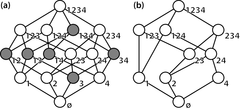
Let $e_{1},e_{2},\ldots,e_{n}$ denote the set of events. All combinations of events are regarded as a partially ordered set and form a complete hierarchy (Figure 1a). Amari introduced the orthogonal decomposition of probability distributions defined on the complete hierarchy of events [1]. That method provided a theoretical foundation with which to analyze the higher-order interactions in a wide variety of applications, such as firing patterns of neurons [2, 3], gene interactions [4], and word associations in documents [5]. However, in many applications the hierarchy is often incomplete, because some event combinations can never occur (Figure 1b). For example, if $e_{1}$ indicates a person being male and $e_{2}$ indicates a person having ovarian cancer, the combination of $e_{1}$ and $e_{2}$ can never occur. Incomplete hierarchies can also result from a lack of data [6].

We define information geometric dual coordinates on a partially ordered set, or a poset. They lead to an efficient algorithm for decomposing Kullback–Leibler divergence and entropy in an incomplete hierarchy. Our method can be used to isolate the contribution of each event combination and assess its statistical significance [2]. From a theoretical viewpoint, our method offers a previously unexplored link between order theory and information geometry.

The remainder of this paper is organized as follows. Section II introduces a dually flat manifold on a poset. In Section II-A, we show that, given a poset we introduce, the manifold of probability distributions will always have the same dually flat structure as that of the exponential family of the original variable set (Equations (3) and (5)). In Section II-B, we present an efficient algorithm to decompose information on a poset (Algorithms 1, 2 and Theorem 1). As a representative application, in Section III, we show that our algorithm can efficiently isolate information of arbitrary order interactions of events. We summarize and conclude the paper in Section IV.

Figure 1: Hierarchy of combinations of four events $e_{1},e_{2},e_{3}$, and $e_{4}$. Numbers denote corresponding events. (a) The complete hierarchy of combinations of events. (b) Incomplete hierarchy by removing gray combinations in (a).

II Dually Flat Manifold on Posets

Suppose that $X$ is a discrete random variable and $p(x)=\Pr(X=x)$ with $x\in S$ is a probability mass function on a finite set $S$. In information geometry [1, 7], each distribution is treated as a mapping $p{:}S\to\mathbb{R}$ and the set of all probability distributions is understood to be a $(|S|-1)$-dimensional manifold $\boldsymbol{\mathcal{S}}=\{\,p\mid p(x)>0\text{ for all }x\in S,\hskip 5.0pt\sum_{x\in S}p(x)=1\,\}$, where probabilities form a coordinate system of $\boldsymbol{\mathcal{S}}$, called the $p$-coordinate system. Information geometry gives us two more coordinate systems of $\boldsymbol{\mathcal{S}}$, the $\theta$-coordinate system and the $\eta$-coordinate system, which are known to be dually orthogonal and key to decomposing KL divergence via the mixed coordinate system of $\theta$ and $\eta$. We introduce such two coordinates in Section II-A and show decomposition of KL divergence in Section II-B.

We consider the case where $S$ is a partially ordered set, or a poset, which is one of the most fundamental structured space in computer science and mathematics. A partial order “$\leq$” satisfies the following three properties: for all $x,y,z\in S$, (1) $x\leq x$ (reflexivity), (2) $x\leq y$, $y\leq x\Rightarrow x=y$ (antisymmetry), and (3) $x\leq y$, $y\leq z\Rightarrow x\leq z$ (transitivity). Throughout the paper, we assume that $S$ is always finite and includes the bottom element $\bot\in S$; that is, $\bot\leq x$ for all $x\in S$. We write the set $S\setminus\{\bot\}$ by $S^{+}$.

For a subset $I\subseteq S$, we denote a lower set ${\downarrow}I=\{\,x\in S\mid x\leq s\text{ for some }s\in I\,\}$, an upper set ${\uparrow}I=\{\,x\in S\mid x\geq s\text{ for some }s\in I\,\}$, and ${\downarrow}x={\downarrow}\{x\}$, ${\uparrow}x={\uparrow}\{x\}$ for each $x\in S$. In order theory, ${\downarrow}x$ is called the principal ideal for $x$ and ${\uparrow}x$ is called the principal filter for $x$ [8, 9], which are known to be fundamental mathematical objects in posets.

II-A $\theta$- and $\eta$-coordinate Systems

Let us first introduce the $\theta$-coordinate system of the manifold $\boldsymbol{\mathcal{S}}$, which is realized as a mapping $\theta{:}S\to\mathbb{R}$. In the exponential family, $\theta$ is known to be the natural parameter, which is treated as an $n$-dimensional vector $\boldsymbol{\theta}=(\theta^{1},\theta^{2},\dots,\theta^{n})$ and the distribution is in the form of

$$p(x;\boldsymbol{\theta})=\exp\left(\,\sum_{i=1}^{n}\theta^{i}F_{i}(x)-\psi(\boldsymbol{\theta})\,\right)$$ (1)

with $n$ functions $F_{1},\dots,F_{n}$ and a normalizer $\psi(\boldsymbol{\theta})$ [7]. This is re-written as

$$p(x;\theta)=\exp\left(\,\sum_{s\in S^{+}}\theta(s)F_{s}(x)-\psi(\theta)\,\right)$$ (2)

with $n=|S^{+}|$ in our setting, where there exists a one-to-one indexing mapping $\omega{:}S^{+}\to\{1,2,\dots,n\}$ such that $\theta(s)$ and $F_{s}$ correspond to $\theta^{\omega(s)}$ and $F_{\omega(s)}$ in Equation (1), respectively.

Given a poset $S$, we propose to define $F_{s}(x)$ as

$$F_{s}(x) =\left\{\begin{array}[]{ll}1&\text{if }s\leq x,\\ 0&\text{otherwise}\end{array}\right.\ \text{and}\ \psi(\theta)=-\log p(\bot).$$

Interestingly, from Equation (2), we obtain the expansion of $\log p(x)$ as the sum of $\theta(s)$ of lower elements $s\leq x$ in $S$:

$$\log p(x)=\sum_{s\leq x}\theta(s).$$ (3)

Note that this equation can be viewed as a generalization of the well-known log-linear model:

$$\log p(\boldsymbol{x})= \sum_{i}\theta^{i}x^{i}+\sum_{i<j}\theta^{ij}x^{i}x^{j}+\sum_{i<j<k}\theta^{ijk}x^{i}x^{j}x^{k}$$

$$+\dots+\theta^{1\dots n}x^{1}\dots x^{n}-\psi$$

for $n$-dimensional binary vector $\boldsymbol{x}=(x^{1},\dots,x^{n})\in\{0,1\}^{n}$.

Thus, given a probability distribution $p\in\boldsymbol{\mathcal{S}}$, the $\theta$-coordinate system $\theta{:}S\to\mathbb{R}$ is recursively computed as

$$\theta(x)=\log p(x)-\displaystyle\sum_{s<x}\theta(s)$$ (4)

starting from the bottom $\theta(\bot)=\log p(\bot)$.

Figure 2: $p(x)$, $\theta(x)$, and $\eta(x)$ on poset.

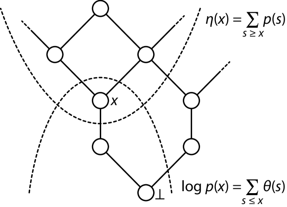
In information geometry [1], the natural parameter $\theta$ of the exponential family is known to be the $e$-affine coordinate of the $e$-flat manifold $\boldsymbol{\mathcal{S}}$, which means that our formulation of $\theta$ in Equation (4) is the $e$-affine coordinate. The $m$-affine coordinate $\eta{:}S\to\mathbb{R}$, an alternative coordinate system that introduces the duality to $\boldsymbol{\mathcal{S}}$, is given as the expectation of the parameter $F_{s}(x)$ for each $s\in S$. In our case $\eta$ is given as follows:

$$\eta(s)=\mathbb{E}[F_{s}(x)]=\sum_{x\geq s}p(x)=\Pr(X\geq s).$$ (5)

Relationships of $p$, $\theta$, and $\eta$ are illustrated in Figure 2.

The two coordinate systems $\theta$ and $\eta$ are connected with each other by the Legendre transformation. The remarkable property is that $\theta$ and $\eta$ are dually orthogonal:

$$\mathbb{E}\left[\,\frac{\partial}{\partial\theta(s)}\log p(x;\theta)\frac{\partial}{\partial\eta(s^{\prime})}\log p(x;\eta)\,\right]=\delta(s,s^{\prime})$$ (6)

for every $s,s^{\prime}\in S^{+}$ with the Kronecker delta $\delta$ such that $\delta(s,s^{\prime})=1$ if $s=s^{\prime}$ and $\delta(s,s^{\prime})=0$ otherwise [1]. This property is essential to construct a mixed coordinate system of $\theta$ and $\eta$ in the next subsection.

Our finding connects two fundamental areas, information geometry and order theory, that have been independently studied to date. Given the $\theta$-coordinate, our result means that the $p$-coordinate is generated from the set of principal ideals and the $\eta$-coordinate is generated from the set of principal filters. More specifically, let $f(I,\theta)=\exp(\,\sum_{s\in I}\theta(s)\,)$ and $g(I,p)=\sum_{s\in I}p(s)$ for every $I\subseteq S$. For each $x\in S$, we have $p(x)=f({\uparrow}x,\theta)$ with the principal ideal ${\uparrow}x$ for $x$ and $\eta(x)=g({\downarrow}x,p)$ with the principal filter ${\downarrow}x$.

II-B Information Decomposition via Mixed Coordinate System

We introduce the mixed coordinate system of $\theta$ and $\eta$ [1] on a poset, the key tool to analyze distributions on $S$. The mixed coordinate system $\xi_{I}:S^{+}\to\mathbb{R}$ with respect to a subset $I\subseteq S^{+}$ is a coordinate system of $\boldsymbol{\mathcal{S}}$ such that

$$\xi_{I}(x)\coloneqq\left\{\begin{array}[]{ll}\eta(x)&\text{if }x\in S^{+}\setminus I,\\ \theta(x)&\text{if }x\in I.\end{array}\right.$$

Using the system, we can blend two distributions $p$ and $q$: The mixed distribution of a pair of distributions $(p,q)$ with respect to $I\subseteq S^{+}$ is the distribution $r\in\boldsymbol{\mathcal{S}}$ such that

$$\left\{\begin{array}[]{ll}\eta_{r}(x)=\eta_{p}(x)&\text{if }x\in S^{+}\setminus I,\\ \theta_{r}(x)=\theta_{q}(x)&\text{if }x\in I,\end{array}\right.$$

and $r(\bot)=1-\sum_{s\in S^{+}}r(x)$, where we write $\theta$- and $\eta$-coordinates corresponding to $p$ by $\theta_{p}$ and $\eta_{p}$, respectively, to clarify that $p$, $\theta_{p}$, and $\eta_{p}$ are the same point in $\boldsymbol{\mathcal{S}}$. Due to the orthogonality of $\theta$ and $\eta$ in Equation (6), this distribution is always unique and well-defined.

Figure 3: Pythagoras theorem (Theorem 1).

Here we show decomposition of the Kullback–Leibler (KL) divergence between two probability distributions $p,q$:

$$D_{\mathrm{KL}}(p,q)=\sum_{x\in S}p(x)\log\frac{p(x)}{q(x)}$$ (7)

using their mixed distribution $r$.

Theorem 1 (Pythagoras theorem).

Given two distributions $p,q\in\boldsymbol{\mathcal{S}}$ and $I\subseteq S^{+}$. For a mixed distribution $r$ of $(p,q)$ and $r^{\prime}$ of $(q,p)$ with respect to $I$,

$$D_{\mathrm{KL}}(p,q) =D_{\mathrm{KL}}(p,r)+D_{\mathrm{KL}}(r,q),$$ (8)

$$D_{\mathrm{KL}}(q,p) =D_{\mathrm{KL}}(q,r^{\prime})+D_{\mathrm{KL}}(r^{\prime},p).$$ (9)

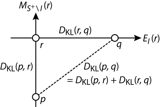
• We can directly use Theorem 3 in [1], which shows that $D_{\mathrm{KL}}(p,q)=D_{\mathrm{KL}}(p,r)+D_{\mathrm{KL}}(r,q)$ holds if $m$-geodesic connecting $p$ and $r$ is orthogonal at $r$ to the $e$-geodesic connecting $r$ and $q$. Let two submanifolds $E_{I}(p)$ and $M_{I}(p)$ of $\boldsymbol{\mathcal{S}}$ be

  $$E_{I}(r) \coloneqq\left\{\,\nu\in\boldsymbol{\mathcal{S}}\mid\theta_{\nu}(x)=\theta_{r}(x)\text{ for all }x\in I\,\right\},$$

  $$M_{S^{+}\setminus I}(r) \coloneqq\left\{\,\nu\in\boldsymbol{\mathcal{S}}\mid\eta_{\nu}(x)=\eta_{r}(x)\text{ for all }x\in S^{+}\setminus I\,\right\}.$$

  Since $E_{I}(r)$ and $M_{S^{+}\setminus I}(r)$ are complementary and orthogonally intersect at $r$ from Equation (6), connection of $p$ and $r$ (resp. $r$ to $q$) is clearly $m$-geodesic (resp. $e$-geodesic; Figure 3). Therefore $D_{\mathrm{KL}}(p,q)=D_{\mathrm{KL}}(p,r)+D_{\mathrm{KL}}(r,q)$ follows. The second equation $D_{\mathrm{KL}}(q,p)=D_{\mathrm{KL}}(q,r^{\prime})+D_{\mathrm{KL}}(r^{\prime},p)$ can be proved in the same way. ∎

Moreover, for a hierarchical collection $\{I_{0},I_{1},\dots,I_{k}\}$ of subsets of $S$ such that $\emptyset=I_{0}\subseteq I_{1}\subseteq\dots\subseteq I_{k}=S^{+}$,

$$D_{\mathrm{KL}}(p,q)=\sum_{i=1}^{k}D_{\mathrm{KL}}(r_{i-1},r_{i}),$$ (10)

where $r_{i}$ is the mixed distribution of $(p,q)$ with respect to $I_{i}$ for each $i\in\{0,1,\dots,k\}$. Note that $r_{0}=p$ and $r_{k}=q$.

Let $p_{0}$ be the uniform distribution such that $p_{0}(x)=1/|S|$ for all $x\in S$, which is the origin of the $\theta$-coordinate because $\theta_{p_{0}}(x)=0$ for all $x\in S^{+}$. Since for the entropy $H(X)$ with a probability distribution $p$

$$H(X)=-\sum_{x\in S}p(x)\log p(x)=\log|S|-D_{\mathrm{KL}}(p,p_{0})$$

holds and $\log|S|$ is a constant, entropy decomposition is achieved by our KL divergence decomposition in Theorem 1:

$$H(X)=\log|S|-\left(\,D_{\mathrm{KL}}(p,r)+D_{\mathrm{KL}}(r,p_{0})\,\right),$$

where $r$ is the mixed distribution of $(p,p_{0})$ with respect to $I\subseteq S^{+}$. The entropy is decomposed into the contribution $D_{\mathrm{KL}}(p,r)$ of elements in $I$ and the other $D_{\mathrm{KL}}(r,p_{0})$. We can therefore obtain the information gain for every subset $I\in S$ as the KL divergence $D_{\mathrm{KL}}(p,p_{I})$, where $p_{I}$ is the mixed distribution of $(p,p_{0})$ with respect to $I$.

II-C Computation of Mixed Distributions

1

2ComputeMixedSingle($x^{*}$)

3       Let $x_{1},\dots,x_{m}=x^{*}$ be the topological ordering of ${\downarrow}x^{*}$

4       Search $r(x^{*})$ that gives $\theta_{r}(x^{*})=\theta_{q}(x^{*})$ using ComputeThetaSingle($x^{*},r(x^{*})$) (e.g. bisection method)

5       return $r$

6 ComputeThetaSingle($x^{*},r(x^{*})$)

7       foreach $s\in{\downarrow}x^{*}$ do // Initializing flags indicating

8             $f(s)\leftarrow 0$ // whether objects are already visited

9       for $i\leftarrow m-1$ to $1$ do

10             $r(x_{i})\leftarrow{}$ComputePSingle($x_{i}$)

11       for $i\leftarrow 1$ to $m$ do

12             Compute $\theta_{r}(x_{i})$

13       return $\theta_{r}(x^{*})$

14      

15 ComputePSingle($x$)

16       $r(x)\leftarrow p(x)$

17       foreach $s\gtrdot x$ do // $x\lessdot s$ iff $x<s$, $x\leq y<s\Rightarrow x=y$

18             $r(x)\leftarrow r(x)+{}$AggregateDiff($s,\omega(x)$) // $\omega(x)$: index of $x$

19       return $r(x)$

20      

21 AggregateDiff($x,i$)

22       if $f(x)=i$ or $x\not\leq x^{*}$ then

23             $p_{\text{diff}}\leftarrow 0$

24      else

25             $f(x)\leftarrow i$

26             $p_{\text{diff}}\leftarrow p(x)-r(x)$

27             foreach $s\gtrdot x$ do

28                   $p_{\text{diff}}\leftarrow p_{\text{diff}}+{}$AggregateDiff($s,i$)

29            

30       return $p_{\text{diff}}$

Algorithm 1 Compute the mixed distribution $r$ of $(p,q)$ with respect to a singleton $I=\{x^{*}\}$

1

2ComputeMixedMulti($I$)

3       repeat

4             for $x^{*}\in I$ do

5                   ComputeMixedSingle($x^{*}$) // Algorithm 1

6            

7      until convergence of $r$;

Algorithm 2 Compute the mixed distribution $r$ of $(p,q)$ with respect to $I\subseteq S^{+}$

Here, we show how to compute the mixed distribution $r$ from $p$ and $q$ with a subset $I\subseteq S^{+}$ . First we present an algorithm to compute $r$ in a simple case, where $I$ is a singleton and we let $I=\{x^{*}\}$. Since $\eta_{r}(x)=\eta_{p}(x)$ for all $x\not=x^{*}$, it is clear that $r(x)=p(x)$ for any $x\not\leq x^{*}$. Therefore, we have focused on computing only $r(x)$ with $x\leq x^{*}$.

Assume $r(x^{*})$ is fixed and let $I_{\geq x}=\{\,s\in{\downarrow}x^{*}\mid s\geq x\,\}$ and $I_{>x}=I_{\geq x}\setminus\{x\}$. For each $x\in{\downarrow}x^{*}$ with $x\not=x^{*}$, we have $\sum_{s\in I_{\geq x}}p(s)=\sum_{s\in I_{\geq x}}r(s)$ from $\eta_{p}(x)=\eta_{r}(x)$. Hence $r(x)$ is obtained as $r(x)=p(x)+\sum_{s\in I_{>x}}\left(\,p(s)-r(s)\,\right)$. Thus if ${\downarrow}x^{*}$ is topologically sorted as $x_{0},x_{1},\dots,x_{m}$ with $x_{0}=\bot$ and $x_{m}=x^{*}$, we can compute $r(x_{m})$, $r(x_{m-1})$, $\dots$, $r(x_{0})$ one after another. The function ComputePSingle$(x)$ in Algorithm 1 performs for this computation. Since $\theta_{r}(x_{0})$, $\theta_{r}(x_{1})$, $\dots$, $\theta_{r}(x_{m})=\theta_{r}(x^{*})$ can be computed after computing all $r(x)$ under fixed $r(x^{*})$, $\theta_{r}(x^{*})$ is numerically computed as a function of $r(x^{*})$. This process is summarized in the function ComputeThetaSingle$(x^{*},r(x^{*}))$ in Algorithm 1. As the function is continuous, we can use a numerical optimization method, such as the bisection method, to efficiently search $r(x^{*})$ giving the solution $\theta_{r}(x^{*})=\theta_{q}(x^{*})$. The time complexity of computing $r$ is $O(h(x^{*})|{\downarrow}x^{*}|^{2})\leq O(h(x^{*})|S|^{2})$, where $h(x^{*})$ is the number of iterations for solving $\theta_{r}(x^{*})=\theta_{q}(x^{*})$.

We next consider the general case. Let $I=\{x_{1}^{*},\dots,x_{l}^{*}\}$. Although it is again difficult to analytically compute the mixed distribution $r$, we can numerically compute the distribution $r$ by iterating computation of $\theta_{r}(x_{i}^{*})$ for each $x_{i}^{*}$ while fixing $\theta(x_{j}^{*})$ with $j\not=i$, which is inspired by alternating optimization over $I$ mainly used in the field of convex optimization. The overall process is shown in Algorithm 2.

Lemma 1.

Algorithm 2 always converges to the mixed distribution $r\in\boldsymbol{\mathcal{S}}$ of $(p,q)$ with respect to $I\subseteq S^{+}$.

• Let $r_{1},r_{2},\dots$ be a sequence of distributions in which each $r_{i}$ is obtained by the $i$th run of the function ComputeMixedSingle in Algorithm 2. From Theorem 1, we have $D_{\mathrm{KL}}(r_{i},r)=D_{\mathrm{KL}}(r_{i},r_{i+1})+D_{\mathrm{KL}}(r_{i+1},r)$ for all $i$, hence $D_{\mathrm{KL}}(r_{i},r)\geq D_{\mathrm{KL}}(r_{i+1},r)$ with the equality holding only if $D_{\mathrm{KL}}(r_{i},r_{i+1})=0$. Since there always exists $r_{j}$ with $j>i$ such that $D_{\mathrm{KL}}(r_{i},r_{j})>0$ if $D_{\mathrm{KL}}(r_{i},r)>\epsilon$ for any $\epsilon>0$, Algorithm 2 converges to the mixed distribution $r$. ∎

Since the time complexity of computing $r(x^{*})$ for each $x^{*}\in I$ is $O(h(x^{*})|{\downarrow}x^{*}|^{2})$, the overall time complexity of computing $r$ is $O(h\sum_{x^{*}\in I}h(x^{*})|{\downarrow}x^{*}|^{2})\leq O(h|S|^{3}\sum_{x^{*}\in I}h(x^{*}))$, where $h$ is the number of iterations until convergence of $r$.

II-D Measuring Statistical Significance of $\theta$

Given a distribution $p$ on $S$, we can assess the statistical significance of $\theta_{p}$ through a likelihood-ratio test, in particular a $G$-test, using decomposition of the KL divergence. Each $\theta_{p}(x)$ shows a contribution of $x$ on $p$ as it is the coefficient of the log expansion of $p$ and is orthogonal to the marginals $\eta_{p}$.

The null and the alternative hypotheses are [2, 4]:

$$H_{0}\!\colon\theta_{p}(x)=0,\forall x\in I,\hskip 10.0ptH_{1}\!\colon\theta_{p}(x)\not=0,\forall x\in I,$$

which means that we knock down all elements $x\in I$ by letting $\theta_{p}(x)=0$ in the generalized log-linear model $\log p(x)=\sum_{s\leq x}\theta_{p}(s)$ in Equation (3). The statistics $\lambda$ is then given as

$$\lambda=2N\sum_{s\in S}\left(\,p(s)\log\left(\,\frac{p(s)}{r(s)}\,\right)\,\right)=2ND_{\mathrm{KL}}(p,r),$$

where $N$ is the sample size and $r$ is the null distribution, the mixed distribution of $(p,p_{0})$ with respect to $I$, and hence $\lambda$ can be computed by Algorithms 1 and 2. Therefore, the $p$-value can be obtained from data samples since $\lambda$ is known to follow the $\chi^{2}$-distribution with the degrees of freedom $|S|-1$.

III Orthogonal Decomposition of Interactions

As a representative application, let us consider the problem of orthogonal decomposition of event combinations. Suppose there are $n$ events $e_{1},\dots,e_{n}$ as discussed in the Introduction. For each subset $x\subseteq[n]=\{1,\dots,n\}$, let $p(x)$ be the probability of the combination $\bigcap_{i\in x}e_{i}$. The objective is to decompose $\log p(x)$ to the sum of coefficients of its subsets $s\subseteq x$, which correspond to the $\theta$-coordinates: $\log p(x)=\sum_{s\leq x}\theta(s)$. The order $\leq$ is given according to the inclusion relationship: $x\leq s$ if $x\subseteq s$. The coefficients $\theta(s)$ show the “pure” contributions of respective interactions $\bigcap_{j\in s}e_{j}$ as they are independent of their frequencies; that is, the $\eta$-coordinates: $\eta(s)=\sum_{x\geq s}p(x)$

Assume that $N$ samples $t_{1},t_{2},\dots,t_{N}$ are given, where each sample $t_{i}$ is a set of events, which means that the events occur simultaneously. We estimate each probability $p(x)$ through its natural estimator $\hat{p}(x)=|\{i\in[N]\mid t_{i}=x\}|\,/\,N$. To effectively estimate $\hat{p}$ and efficiently compute $\theta_{\hat{p}}$ and $\eta_{\hat{p}}$ from samples, we prune the whole event combinations $\mathcal{P}([n])$ by excluding combinations that do not frequently appear in the dataset. Given a threshold $\sigma\in\mathbb{R}$ such that $0\leq\sigma\leq 1$, we set $S^{+}=\{\,x\subseteq[n]\mid\hat{p}(x)\geq\sigma\,\}$ and $\hat{p}(\bot)=1-\sum_{x\in S^{+}}\hat{p}(x)$. Thus the dimensionality of the manifold $\boldsymbol{\mathcal{S}}$ reduces from $2^{n}$ to at most $N$. Since any subset of $\mathcal{P}([n])$ is a poset, we can apply our decomposition technique presented in Section II via computation of $\theta_{\hat{p}}$, $\eta_{\hat{p}}$, and mixed distributions. Interestingly, a sample $t_{i}$ can be viewed as a transaction of a database and $\eta_{\hat{p}}(I)$ corresponds to the support of $I$ used in the context of frequent pattern (itemset) mining [10].

TABLE I: Samples in Example 1.

	Events
$t_{1}$	$e_{2}$
$t_{2}$	$e_{2}$
$t_{3}$	$e_{4}$, $e_{5}$
$t_{4}$	$e_{1}$, $e_{2}$, $e_{4}$, $e_{5}$
$t_{5}$	$e_{1}$, $e_{2}$, $e_{4}$, $e_{5}$
$t_{6}$	$e_{3}$
$t_{7}$	$e_{1}$, $e_{2}$, $e_{4}$, $e_{5}$
$t_{8}$	$e_{4}$, $e_{5}$
$t_{9}$	$e_{1}$, $e_{2}$, $e_{4}$, $e_{5}$
$t_{10}$	$e_{2}$

Figure 4: Poset generated from samples in Table 4.

Example 1.

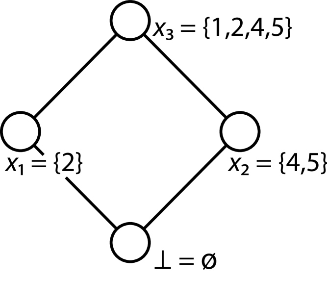
Given samples in Table 4, assume that our threshold $\sigma=0.2$. We then obtain a poset $S=\{\bot,x_{1},x_{2},x_{3}\}$ with $\bot=\emptyset$, $x_{1}=\{2\}$, $x_{2}=\{4,5\}$, and $x_{3}=\{1,2,4,5\}$, as shown in Figure 4, where $\hat{p}(\bot)=0.1$, $\hat{p}(x_{1})=0.3$, $\hat{p}(x_{2})=0.2$, and $\hat{p}(x_{3})=0.4$. Thus, $\theta_{\hat{p}}$ are obtained as follows: $\theta_{\hat{p}}(\bot)=-2.303$, $\theta_{\hat{p}}(x_{1})=1.099$, $\theta_{\hat{p}}(x_{2})=0.693$, and $\theta_{\hat{p}}(x_{3})=-0.405$. Let $\hat{r}_{x}$ be the mixed distribution of $(\hat{p},p_{0})$ with $\{x\}\in S$. From these parameters, the KL divergence for each interaction is obtained as $D_{\mathrm{KL}}(\hat{p},\hat{r}_{x_{1}})=0.0523$, $D_{\mathrm{KL}}(\hat{p},\hat{r}_{x_{2}})=0.0170$, and $D_{\mathrm{KL}}(\hat{p},\hat{r}_{x_{3}})=0.0040$. Although $p$-values of those interactions are larger than $0.99$, they are due to small sample size $N=10$. If $N=300$, for example, the $p$-value of $x_{1}$ becomes $0.001$ and it is significant under the significance level $\alpha=0.05$.

The same strategy can be applied to a poset $S$ composed of vectors of $n$-dimensional nonnegative integers $\mathbb{Z}^{n}_{\geq 0}$. We assume $S$ to be a subset of $\mathbb{Z}^{n}_{\geq 0}$, where for each pair of vectors $x,y\in\mathbb{Z}^{n}_{\geq 0}$ with $\boldsymbol{x}=(x^{1},x^{2},\dots,x^{n})$ and $\boldsymbol{y}=(y^{1},y^{2},\dots,y^{n})$, we define the partial order $\leq$ as $\boldsymbol{x}\leq\boldsymbol{y}$ if and only if $x^{i}\leq y^{i}$ for all $i\in[n]$, and $0=(0,0,\dots,0)\in\mathbb{Z}^{n}_{\geq 0}$ corresponds to $\bot$. Any subset $S\subset\mathbb{Z}^{n}_{\geq 0}$ becomes a poset.

Given $N$ data points $\boldsymbol{x}_{1},\boldsymbol{x}_{2},\dots,\boldsymbol{x}_{N}$ of $n$-dimensional nonnegative integers. Similar to the previous case, a poset $S^{+}$ is obtained from data as $S^{+}=\{\,\boldsymbol{x}\in\mathbb{Z}^{n}_{\geq 0}\mid\hat{p}(\boldsymbol{x})\geq\sigma\,\}$ using a threshold $\sigma\in\mathbb{R}$. We can apply our information decomposition to $S$ with an empirical probability distribution $\hat{p}$.

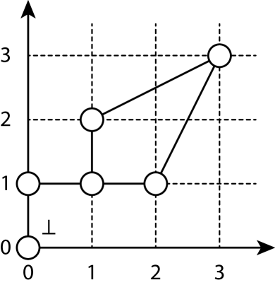
Example 2.

Given data points $\boldsymbol{x}_{1},\boldsymbol{x}_{2},\dots,\boldsymbol{x}_{25}\in\mathbb{Z}^{2}_{\geq 0}$ as $\boldsymbol{x}_{1},\dots,\boldsymbol{x}_{3}=(0,1)$, $\boldsymbol{x}_{4}=(1,0)$, $\boldsymbol{x}_{5},\dots,\boldsymbol{x}_{8}=(1,1)$, $\boldsymbol{x}_{9},\dots,\boldsymbol{x}_{11}=(1,2)$, $\boldsymbol{x}_{12},\dots,\boldsymbol{x}_{21}=(2,1)$, $\boldsymbol{x}_{22},\dots,\boldsymbol{x}_{25}=(3,3)$. We have $S=\{(0,0),(0,1),(1,1),(1,2),(2,1),(3,3)\}$ if $\sigma=2/25$, which is shown in Figure 5.

Figure 5: Poset of nonnegative integer vectors in Example 2.

IV Conclusion

In this paper, we have theoretically shown the intriguing relationship between two key structures in information geometry and order theory: the dually flat structure of a manifold of the exponential family and the partial order structure of events. We have proposed an efficient algorithm of information decomposition that is applicable to any kind of posets; this is in contrast to a number of other studies [11, 12, 13, 14].

As a representative application, we have demonstrated orthogonal decomposition of interactions of events. We have shown that the partial order structure can be directly obtained from data in an efficient manner, and the dimensionality of the manifold is reduced from $2^{n}$ for $n$ variables in previous approaches to, at most, the sample size $N$. Thus, we can perform orthogonal decomposition for recently emerging high-dimensional data with thousands or even millions of variables, such as single nucleotide polymorphisms (SNPs) in genome-wide association studies (GWAS) [15] and neural data in neuroscience [16]. To our knowledge, this is the first method that avoids the curse of dimensionality in orthogonal decomposition of interactions and achieves efficient computation and effective probability estimation from data.

Our work promises many interesting future studies, both in theoretical and practical directions. There will be a more interesting theoretical connection between information geometry and order theory. Furthermore, it is exciting to apply our decomposition method to real-world scientific datasets such as firing patterns of neurons and SNPs in GWAS to reveal unknown associations.

References

- [1] S. Amari, “Information geometry on hierarchy of probability distributions,” IEEE Transactions on Information Theory, vol. 47, no. 5, pp. 1701–1711, 2001.
- [2] H. Nakahara and S. Amari, “Information-geometric measure for neural spikes,” Neural Computation, vol. 14, no. 10, pp. 2269–2316, 2002.
- [3] H. Nakahara, S. Amari, and B. J. Richmond, “A comparison of descriptive models of a single spike train by information-geometric measure,” Neural computation, vol. 18, no. 3, pp. 545–568, 2006.
- [4] H. Nakahara, S. Nishimura, M. Inoue, G. Hori, and S. Amari, “Gene interaction in DNA microarray data is decomposed by information geometric measure,” Bioinformatics, vol. 19, no. 9, pp. 1124–1131, 2003.
- [5] Y. Hou, X. Zhao, D. Song, and W. Li, “Mining pure high-order word associations via information geometry for information retrieval,” ACM Transactions on Information Systems, vol. 31, no. 3, pp. 12:1–12:32, 2013.
- [6] E. Ganmor, R. Segev, and E. Schneidman, “Sparse low-order interaction network underlies a highly correlated and learnable neural population code,” Proceedings of the National Academy of Sciences, vol. 108, no. 23, pp. 9679–9684, 2011.
- [7] S. Amari and H. Nagaoka, Methods of information geometry. American Mathematical Society, 2007.
- [8] B. A. Davey and H. A. Priestley, Introduction to lattices and order, 2nd ed. Cambridge University Press, 2002.
- [9] G. Gierz, K. H. Hofmann, K. Keimel, J. D. Lawson, M. Mislove, and D. S. Scott, Continuous Lattices and Domains. Cambridge University Press, 2003.
- [10] C. C. Aggarwal and J. Han, Eds., Frequent Pattern Mining. Springer, 2014.
- [11] N. Bertschinger, J. Rauh, E. Olbrich, and J. Jost, “Shared information—new insights and problems in decomposing information in complex systems,” in Proceedings of the European Conference on Complex Systems 2012. Springer, 2013, pp. 251–269.
- [12] N. Bertschinger, J. Rauh, E. Olbrich, J. Jost, and N. Ay, “Quantifying unique information,” Entropy, vol. 16, no. 4, pp. 2161–2183, 2014.
- [13] E. Olbrich, N. Bertschinger, and J. Rauh, “Information decomposition and synergy,” Entropy, vol. 17, no. 5, pp. 3501–3517, 2015.
- [14] P. L. Williams and R. D. Beer, “Nonnegative decomposition of multivariate information,” arXiv:1004.2515, 2010.
- [15] The Wellcome Trust Case Control Consortium, “Genome-wide association study of 14,000 cases of seven common diseases and 3,000 shared controls,” Nature, vol. 447, no. 7145, pp. 661–678, 2007.
- [16] A. Alivisatos, M. Chun, G. Church, R. Greenspan, M. Roukes, and R. Yuste, “The brain activity map project and the challenge of functional connectomics,” Neuron, vol. 74, pp. 970–974, 2012.