Bounds on Tail Probabilities in Exponential families

Abstract

In this paper we present various new inequalities for tail proabilities for distributions that are elements of the most improtant exponential families. These families include the Poisson distributions, the Gamma distributions, the binomial distributions, the negative binomial distributions and the inverse Gaussian distributions. All these exponential families have simple variance functions and the variance functions play an important role in the exposition. All the inequalities presented in this paper are formulated in terms of the signed log-likelihood. The inequalities are of a qualitative nature in that they can be formulated either in terms of stochastic domination or in terms of an intersection property that states that a certain discrete distribution is very close to a certain continuous distribution.

1 Introduction

Let $X_{1},\dots,X_{n}$ be i.i.d. random variables such that the moment generating function $\beta\curvearrowright E[\exp(\beta X_{1})]$ is finite in a neighborhood of the origin. For a fixed value of $\mu$ one is interested in approximating the tail distribution: $\Pr(\sum_{i=1}^{n}X_{i}\leq\mu)$ . If $\mu$ is close to the mean of $X_{1}$ one would usually approximate the tail probability by the tail probability of a Gaussian random variable. If $\mu$ is far from the mean of $X_{1}$ the tail probability can be estimated using large deviation theory. According to the Sanov theorem the probability that the deviation from the mean is as large as $\mu$ is of the order $\exp\left(-D\right)$ where D is a constant or to be more precise

$$-\frac{\ln\left(\Pr(\sum_{i=1}^{n}X_{i}\leq\mu)\right)}{n}\to D$$

for $n\to\infty.$ Bahadur and Rao Bahadur (1960); Bahadur and Rao (1960) improved the estimate of this large deviation probability, and in Györfi et al (2012) such Gaussian tail approximations were extended to situations where one normally uses large deviation techniques.

The distribution of the signed log-likelihood is close to a standard Gaussian for a variety of distributions. An asymptotic result for large sample sizes this is not new Zhang (2008), but in this paper we are interested in inequalities that hold for any sample size. Some inequalities of this type can be found in Alfers1984; Reiczigel et al (2011); Harremoës and Tusnády (2012); Zubkov and Serov (2013); Harremoes2014, but here we attempt to give a more systematic presentation including a number of new or improved inequalities.

In this paper we let $\tau$ denote the circle constant $2\pi$ and $\phi$ will denote the standard Gaussian density

$$\frac{\exp\left(-\frac{x^{2}}{2}\right)}{\tau^{\nicefrac{{1}}{{2}}}}.$$

We let $\Phi$ denote the distribution function of the standard Gaussian

$$\Phi\left(t\right)=\int_{-\infty}^{t}\phi\left(x\right)\,\text{d}x\leavevmode\nobreak\ .$$

The rest of the paper is organized as follows. In Section 2 we define the signed log-likelihood of exponential families and look at some of the fundamental properties of the signed log-likelihood. Next we study inequalities for the signed log-likelihood for certain exponential families associated with continuous waiting times. We start with the inverse Gaussian in Section 3 that is particularly simple. Then we study the exponential distributions (Section 4) and more general Gamma distributions (Section 5). Next we turn our attention to discrete waiting times. First we obtain some new inequalities for the geometric distributions (Section 6) and then we generalize the results to negative binomial distributions (Section 7). The negative binomial distributions are waiting times in Bernoulli processes, so in Section 8 our inequalities between negative binomial distributions and Gamma distributions are translated into inequalities between binomial distributions and Poisson distributions. Combined with our domination inequalities for Gamma distributions we obtain an intersection inequality between binomial distributions and the Standard Gaussian distribution. In this paper the focus is on intersection inequalities and stochastic domination inequalities, but in the discussion we mention some related inequalities of other types and how they may be improved.

2 The signed log-likelihood for exponential families

Consider the 1-dimensional exponential family $P_{\beta}$ where

$$\frac{\text{d}P_{\beta}}{\text{d}P_{0}}\left(x\right)=\frac{\exp\left(\beta\cdot x\right)}{Z\left(\beta\right)}$$

and $Z$ denotes the moment generating function given by Z$\left(\beta\right)=\int\exp\left(\beta\cdot x\right)\,\text{d}P_{0}x.$ Let $P^{\mu}$ denote the element in the exponential family with mean value $\mu,$ and let $\hat{\beta}\left(\mu\right)$ denote the corresponding maximum likelihood estimate of $\beta.$ Let $\mu_{0}$ denote the mean value of $P_{0}$. Then

$$D\left(P^{\mu}\|P_{0}\right) =\int\ln\left(\frac{\text{d}P^{\mu}}{\text{d}P_{0}}\left(x\right)\right)\,\text{d}P^{\mu}x.$$

The variance function of an exponential family is defined so that $V\left(\mu\right)$ is the variance of $P^{\mu}.$ The variance functions uniquely characterizes the corresponding exponential families and most important exponential families have very simple variance functions. If we know the varince function the divergence can be calculated according to the following formula.

Lemma 1

In an exponential family $\left(P^{\mu}\right)$ parametrized by mean value $\mu$and with variance function $V$ information divergence can be calculated according to the formula

$$D\left(P^{\mu_{1}}\|P^{\mu_{2}}\right)=\int_{\mu_{1}}^{\mu_{2}}\frac{\mu-\mu_{1}}{V\left(\mu\right)}\,\mathrm{d}\mu.$$

Proof

The divergence is given by

$$D\left(P^{\mu_{1}}\|P^{\mu_{2}}\right) =\int\ln\left(\frac{\text{d}P^{\mu_{1}}}{\text{d}P^{\mu_{2}}}\left(x\right)\right)\,\text{d}P^{\mu_{1}}x$$

$$=\int\ln\left(\frac{\frac{\exp\left(\beta_{1}\cdot x\right)}{Z\left(\beta_{1}\right)}}{\frac{\exp\left(\beta_{2}\cdot x\right)}{Z\left(\beta_{2}\right)}}\right)\,\text{d}P^{\mu_{1}}x$$

$$=\int\left(\left(\beta_{1}-\beta_{2}\right)x-\ln Z\left(\beta_{1}\right)+\ln Z\left(\beta_{2}\right)\right)\,\text{d}P^{\mu_{1}}x$$

$$=\left(\beta_{1}-\beta_{2}\right)\mu_{1}-\ln Z\left(\beta_{1}\right)+\ln Z\left(\beta_{2}\right).$$

The derivative with respect to $\beta_{2}$ is

$$\frac{\partial}{\partial\beta_{2}}D\left(P^{\mu_{1}}\|P^{\mu_{2}}\right)=\mu_{2}-\mu_{1}.$$

Therefore the derivative with respect to $\mu_{2}$ is

$$\frac{\partial}{\partial\mu_{2}}D\left(P^{\mu_{1}}\|P^{\mu_{2}}\right) =\frac{\mu_{2}-\mu_{1}}{\frac{\mathrm{d}\mu_{2}}{\mathrm{d}\beta_{2}}}$$

$$=\frac{\mu_{2}-\mu_{1}}{V\left(\mu_{2}\right)}.$$

Together with the trivial identity

$$D\left(P^{\mu_{1}}\|P^{\mu_{1}}\right)=\int_{\mu_{1}}^{\mu_{1}}\frac{\mu-\mu_{1}}{V\left(\mu\right)}\,\mathrm{d}\mu$$

the results follows.∎

Definition 1

(From Barndorff-Nielsen (1990)) Let $X$ be a random variable with distribution $P_{0}.$ Then the signed log-likelihood $G\left(X\right)$ of $X$ is the random variable given by

$$G\left(x\right)=\left\{\begin{array}[]{cc}-\left[2D\left(P^{x}\|P_{0}\right)\right]^{\nicefrac{{1}}{{2}}},&\text{for }x<\mu_{0};\\ +\left[2D\left(P^{x}\|P_{0}\right)\right]^{\nicefrac{{1}}{{2}}},&\text{for }x\geq\mu_{0}.\end{array}\right.$$

We will need the following general lemma.

Lemma 2

If the variance function is increasing then

$$\frac{G\left(x\right)}{x-\mu_{0}}$$

is a decreasing function of $x$.

Proof

We have

$$\frac{\mathrm{d}}{\mathrm{d}x}\left(\frac{G\left(x\right)}{x-\mu_{0}}\right) =\frac{\left(x-\mu_{0}\right)\frac{D^{\prime}\left(x\right)}{G\left(x\right)}-G\left(x\right)}{\left(x-\mu_{0}\right)^{2}}$$

$$=\frac{\left(x-\mu_{0}\right)\int_{x}^{\mu_{0}}\frac{-1}{V\left(\mu\right)}\,\mathrm{d}\mu-2D}{\left(x-\mu_{0}\right)^{2}G\left(x\right)}$$

$$=\frac{\left(x-\mu_{0}\right)\int_{\mu_{0}}^{x}\frac{1}{V\left(\mu\right)}\,\mathrm{d}\mu-2D}{\left(x-\mu_{0}\right)^{2}G\left(x\right)}.$$

We have to prove that numerator is positive for $x<\mu_{0}$ and negative for $x>\mu_{0}.$ The numerator can be calculated as

$$\left(x-\mu_{0}\right)\int_{\mu_{0}}^{x}\frac{1}{V\left(\mu\right)}\,\mathrm{d}\mu-2D =\left(x-\mu_{0}\right)\int_{\mu_{0}}^{x}\frac{1}{V\left(\mu\right)}\,\mathrm{d}\mu-2\int_{\mu_{0}}^{x}\frac{\mu-\mu_{0}}{V\left(\mu\right)}\,\mathrm{d}\mu$$

$$=\int_{\mu_{0}}^{x}\left(\frac{x-\mu_{0}}{V\left(\mu\right)}-2\frac{\mu-\mu_{0}}{V\left(\mu\right)}\right)\,\mathrm{d}\mu$$

$$=\int_{\mu_{0}}^{x}\frac{x+\mu_{0}-2\mu}{V\left(\mu\right)}\,\mathrm{d}\mu$$

If $x>\mu_{0}$ then

$$\int_{\mu_{0}}^{x}\frac{x+\mu_{0}-2\mu}{V\left(\mu\right)}\,\mathrm{d}\mu =\int_{\mu_{0}}^{\frac{x+\mu_{0}}{2}}\frac{x+\mu_{0}-2\mu}{V\left(\mu\right)}\,\mathrm{d}\mu+\int_{\frac{x+\mu_{0}}{2}_{0}}^{x}\frac{x+\mu_{0}-2\mu}{V\left(\mu\right)}\,\mathrm{d}\mu$$

$$\geq\int_{\mu_{0}}^{\frac{x+\mu_{0}}{2}}\frac{x+\mu_{0}-2\mu}{V\left(\frac{x+\mu_{0}}{2}\right)}\,\mathrm{d}\mu+\int_{\frac{x+\mu_{0}}{2}_{0}}^{x}\frac{x+\mu_{0}-2\mu}{V\left(\frac{x+\mu_{0}}{2}\right)}\,\mathrm{d}\mu$$

$$=\int_{\mu_{0}}^{x}\frac{x+\mu_{0}-2\mu}{V\left(\frac{x+\mu_{0}}{2}\right)}\,\mathrm{d}\mu=0.$$

The inequality for $x<\mu_{0}$ is proved in the same way. ∎

3 Inequalities for inverse Gaussian

The inverse Gaussian distribution and it is used to model waiting times for a Wiener process (Brownian motion) with drift. An inverse Gaussian distribution has density

$$f\left(w\right)=\left[\frac{\lambda}{\tau w^{3}}\right]^{\nicefrac{{1}}{{2}}}\exp\left(\frac{-\lambda\left(w-\mu\right)^{2}}{2\mu^{2}w}\right)$$

with mean value parameter $\mu$ and shape parameter $\lambda.$ The variance function is $V\left(\mu\right)=\mu^{3}/\lambda.$

The divergence of an inverse Gaussian distribution with mean $\mu_{1}$ from an inverse Gaussian distribution with mean $\mu_{2}$ is

$$\int_{\mu_{1}}^{\mu_{2}}\frac{\mu-\mu_{1}}{\mu^{3}/\lambda}\,d\mu=\frac{\lambda\left(\mu_{1}-\mu_{2}\right)^{2}}{2\mu_{1}\mu_{2}^{2}}.$$

Hence the signed log-likelihood is

$$G_{\mu,\lambda}\left(w\right)=\frac{\lambda^{\nicefrac{{1}}{{2}}}\left(w-\mu\right)}{w^{\nicefrac{{1}}{{2}}}\mu}.$$

We observe that

$$G_{\mu,\lambda}\left(w\right) =\left[\frac{\lambda}{\mu}\right]^{\nicefrac{{1}}{{2}}}\frac{\frac{w}{\mu}-1}{\left[\frac{w}{\mu}\right]^{\nicefrac{{1}}{{2}}}}$$

$$=\left[\frac{\lambda}{\mu}\right]^{\nicefrac{{1}}{{2}}}G_{1,1}\left(\frac{w}{\mu}\right).$$

Note that the saddle-point approximation Daniels (1954) is exact for the family of inverse Gaussian distributions, i.e.

$$f\left(w\right)=\frac{\phi\left(G\left(w\right)\right)}{\left[V\left(w\right)\right]^{\nicefrac{{1}}{{2}}}}.$$

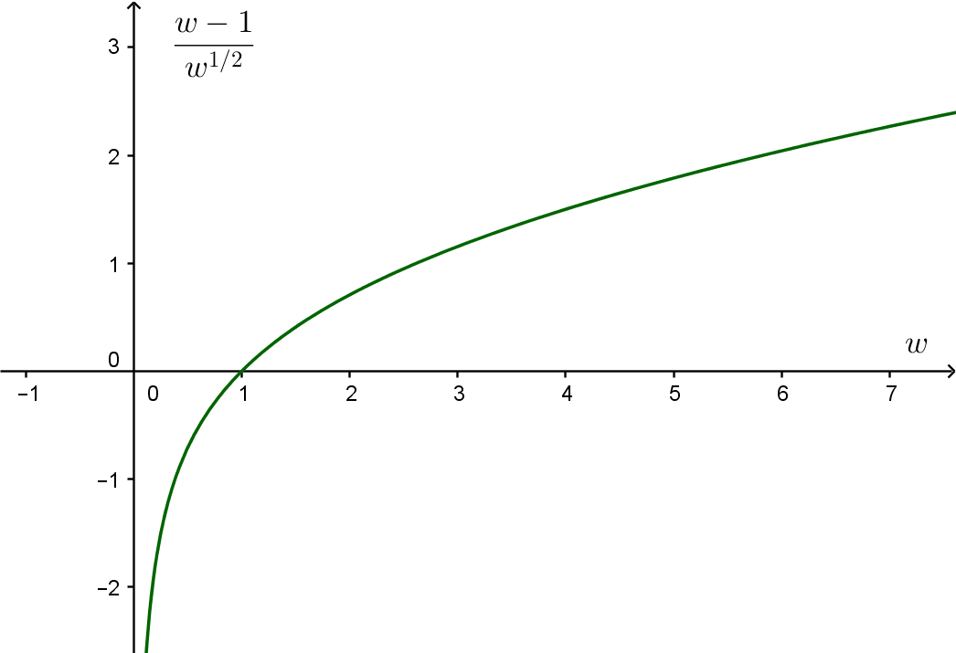
Figure 1: The signed log-likelihood of an inverse Gaussian distribution with mean value 1 and shape parameter 1.

Lemma 3

The probability density of the random variable $G_{\mu,\lambda}\left(W\right)$ is

$$\frac{2\phi\left(z\right)}{1+g^{-1}\left(z\cdot\left[\frac{\mu}{\lambda}\right]^{\nicefrac{{1}}{{2}}}\right)}$$

where $g$ denotes the function $G_{1,1}$.

Proof

The density of $G_{\mu,\lambda}\left(W\right)$ is

$$\frac{f\left(G_{\mu,\lambda}^{-1}\left(z\right)\right)}{G_{\mu,\lambda}^{{}^{\prime}}\left(G_{\mu,\lambda}^{-1}\left(z\right)\right)} =\frac{\frac{\phi\left(G_{\mu,\lambda}\left(G_{\mu,\lambda}^{-1}\left(z\right)\right)\right)}{\left[V\left(G_{\mu,\lambda}^{-1}\left(z\right)\right)\right]^{\nicefrac{{1}}{{2}}}}}{G_{\mu,\lambda}^{{}^{\prime}}\left(G_{\mu,\lambda}^{-1}\left(z\right)\right)}$$

$$=\frac{\phi\left(z\right)}{\left[V\left(G_{\mu,\lambda}^{-1}\left(z\right)\right)\right]^{\nicefrac{{1}}{{2}}}G_{\mu,\lambda}^{{}^{\prime}}\left(G_{\mu,\lambda}^{-1}\left(z\right)\right)}.$$

Now we use that

$$G_{\mu,\lambda}^{{}^{\prime}}\left(w\right) =\frac{w^{\nicefrac{{1}}{{2}}}\mu\lambda^{\nicefrac{{1}}{{2}}}-\nicefrac{{1}}{{2}}\cdot w^{-\nicefrac{{1}}{{2}}}\mu\lambda^{\nicefrac{{1}}{{2}}}\left(w-\mu\right)}{w\mu^{2}}$$

$$=\lambda^{\nicefrac{{1}}{{2}}}\frac{\mu+w}{2w^{\nicefrac{{3}}{{2}}}\mu}.$$

Hence

$$\left[V\left(w\right)\right]^{\nicefrac{{1}}{{2}}}G_{\mu,\lambda}^{{}^{\prime}}\left(w\right) =\left[\frac{w^{3}}{\lambda}\right]^{\nicefrac{{1}}{{2}}}\cdot\lambda^{\nicefrac{{1}}{{2}}}\frac{\mu+w}{2w^{\nicefrac{{3}}{{2}}}\mu}$$

$$=\frac{\mu+w}{2\mu}.$$

Therefore the density of $G_{\mu,\lambda}\left(W\right)$ is

$$f\left(z\right) =\frac{\phi\left(z\right)2\mu}{G_{\mu,\lambda}^{-1}\left(z\right)+\mu}.$$

By isolating $x$ in the equation $G_{\mu,\lambda}\left(x\right)=z$ we get

$$G_{\mu,\lambda}^{-1}\left(z\right)=\mu\cdot G_{1,1}^{-1}\left(z\cdot\left[\frac{\mu}{\lambda}\right]^{\nicefrac{{1}}{{2}}}\right).$$

Hence

$$f\left(z\right)=\frac{\phi\left(z\right)2}{G_{1,1}^{-1}\left(z\cdot\left[\frac{\mu}{\lambda}\right]^{\nicefrac{{1}}{{2}}}\right)+1}\,,$$

which proves the theorem. ∎

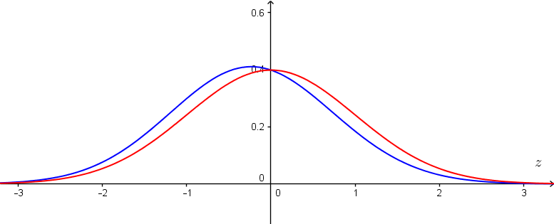
Figure 2: The density of the signed log-likelihood of an inverse Gaussian distribution (blue) with mean value 1 and shape parameter 1 comparead with the density of a standard Gaussian distribution (red).

Lemma 4

(From Harremoës and Tusnády (2012)) Let $X_{1}$ and $X_{2}$ denote random variables with density functions $f_{1}$ and $f_{2}$. If $f_{1}\left(x\right)\geq f_{2}\left(x\right)$ for $x\leq x_{0}$ and $f_{1}\left(x\right)\leq f_{2}\left(x\right)$ for $x\geq x_{0},$ then $X_{1}$ is stochastically dominated by $X_{2}.$ In particular if $\frac{f_{2}\left(x\right)}{f_{1}\left(x\right)}$ is increasing then $X_{1}$ is stochastically dominated by $X_{2}.$

Proof

Assume that $f_{1}\left(x\right)\geq f_{2}\left(x\right)$ for $x\leq x_{0}$ and that $f_{1}\left(x\right)\leq f_{2}\left(x\right)$ for $x\geq x_{0}.$ For $t\geq x_{0}$ we have

$$P\left(X_{1}\geq t\right) =\int_{t}^{\infty}f_{1}\left(x\right)\,dx$$

$$\leq\int_{t}^{\infty}f_{2}\left(x\right)\,dx$$

$$=P\left(X_{2}\geq t\right).$$

Similarly it is proved that $P\left(X_{1}\leq t\right)\geq P\left(X_{2}\leq t\right)$ for $t\leq x_{0}$ but this implies that $P\left(X_{1}>t\right)\leq P\left(X_{2}>t\right).$ If $\frac{f_{2}\left(x\right)}{f_{1}\left(x\right)}$ is increasing then there exist a number $x_{0}$ such that $f_{1}\left(x\right)\geq f_{2}\left(x\right)$ for $x\leq x_{0}$ and that $f_{1}\left(x\right)\leq f_{2}\left(x\right)$ for $x\geq x_{0}.$

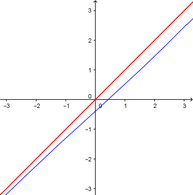
Figure 3: Plot of the quantiles of a standard Gaussian vs. the same quantiles of the signed log-likelihood of the invers Gaussian with $\mu=1$ and $\lambda=1$ .

∎

Theorem 3.1

If $W$ is inverse Gauiisan distributed $IG\left(\mu,\lambda\right)$ then the signed log-likelihood

$$G_{W\left(\mu,\lambda\right)}\left(W\right)$$

is stochastically dominated by the standard Gaussian distribution, i.e. the inequality

$$\Phi\left(G_{W\left(\mu,\lambda\right)}\left(w\right)\right)\leq\Pr\left(W\leq w\right)$$

holds for any $w\in\left]0,\infty\right[$.

Proof

We have to prove that if $W$ has an inverse Gaussian distribution then $G\left(W\right)$ is stochastically dominated by the standard Gaussian. According to Lemma 4 we can prove stochastic dominance by proving that $\phi\left(z\right)/f\left(z\right)$ is increasing. Now

$$\frac{\phi\left(z\right)}{f\left(z\right)}=\frac{g^{-1}\left(z\cdot\left[\frac{\mu}{\lambda}\right]^{\nicefrac{{1}}{{2}}}\right)+1}{2}$$

which is increasing because the function $g$ is increasing. ∎

If Wald random variables are added they become more and more Gaussian and so do their signed log-likelihood. The next theorem states that the convergence of the signed log-likelihood towards the standard Gaussian is monotone in stochastic domination.

Theorem 3.2

Assume that $W_{1}$ and $W_{2}$ have inverse Gaussian distributions let $G_{1}\left(W_{1}\right)$ and $G_{2}\left(W_{2}\right)$ denote their signed log-likelihood. Then $G_{1}\left(W_{1}\right)$ is stochantically dominated by $G_{2}\left(W_{2}\right)$ if and only if $\frac{\mu_{1}}{\lambda_{1}}>\frac{\mu_{2}}{\lambda_{2}}.$

Proof

We have to prove that the densities satisfy

$$\frac{\phi\left(z\right)2}{g^{-1}\left(z\cdot\left[\frac{\mu_{1}}{\lambda_{1}}\right]^{\nicefrac{{1}}{{2}}}\right)+1}<\frac{\phi\left(z\right)2}{g^{-1}\left(z\cdot\left[\frac{\mu_{2}}{\lambda_{2}}\right]^{\nicefrac{{1}}{{2}}}\right)+1}$$

for $z>0$ and the reverse inequality for $z<0.$ The inequality is equivalent to

$$g^{-1}\left(z\cdot\left[\frac{\mu_{1}}{\lambda_{1}}\right]^{\nicefrac{{1}}{{2}}}\right)>g^{-1}\left(z\cdot\left[\frac{\mu_{2}}{\lambda_{2}}\right]^{\nicefrac{{1}}{{2}}}\right).$$

For $z>0$ this follows because the function $g^{-1}$ is increasing. The reversed inequality is proved in the same way. ∎

4 Exponential distributions

Although the tail probabilities of the exponential distribution are easy to calculate the inequalities related to the signed log-likelihood of the exponential distribution are non-trivial and will be useful later.

The exponential distribution $Exp^{\theta}$ has density

$$f\left(x\right)=\frac{1}{\theta}\exp\left(-\frac{x}{\theta}\right).$$

The distribution function is

$$\Pr\left(X\leq x\right)=\int_{0}^{x}\frac{1}{\theta}\exp\left(-\frac{t}{\theta}\right)\,\mathrm{d}t=1-\exp\left(-\frac{x}{\theta}\right).$$

The mean of the exponential distribution $Exp^{\theta}$ is $\theta$ and the variance is $\theta^{2}$ so the variance function is $V\left(\mu\right)=\mu^{2}.$ The divergence can be calculated as

$$D\left(Exp^{\theta_{1}}\|Exp^{\theta_{2}}\right) =\int_{\theta_{1}}^{\theta_{2}}\frac{\mu-\theta_{1}}{\mu^{2}}\,\mathrm{d}\mu$$

$$=\frac{\theta_{1}}{\theta_{2}}-1-\ln\frac{\theta_{1}}{\theta_{2}}.$$

From this we see that

$$G_{Exp^{\theta}}\left(x\right) =\pm\left[2\left(\frac{x}{\theta}-1-\ln\frac{x}{\theta}\right)\right]^{\nicefrac{{1}}{{2}}}$$

$$=\gamma\left(\frac{x}{\theta}\right)$$

where $\gamma$ denotes the function

$$\mbox{$\gamma\left(x\right)$=}\begin{cases}-\left[2\left(x-1-\ln x\right)\right]^{\nicefrac{{1}}{{2}}},&\textrm{when}\,x\leq 1;\\ +\left[2\left(x-1-\ln x\right)\right]^{\nicefrac{{1}}{{2}}},&\textrm{when}\,x>1.\end{cases}$$

Note that the saddle-point approximation is exact for the family of exponential distributions, i.e.

$$f\left(x\right) =\frac{\tau^{\nicefrac{{1}}{{2}}}}{\mathrm{e}}\cdot\frac{\phi\left(G\left(x\right)\right)}{\left[V\left(x\right)\right]^{\nicefrac{{1}}{{2}}}}.$$

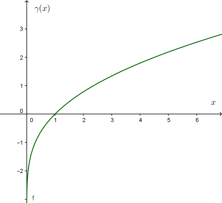
Figure 4: The signed log-likelihood $\gamma\left(x\right)$ of an exponential distribution.

Lemma 5

The density of the signed log-likelihood of an exponential random variable is given by

$$\frac{\tau^{\nicefrac{{1}}{{2}}}}{\mathrm{e}}\cdot\frac{z\phi\left(z\right)}{\gamma^{-1}\left(z\right)-1}.$$

Proof

Let $X$ be a $Exp^{\theta}$ distributed random variable. The density of the signed log-likelihood is

$$\frac{f\left(G^{-1}\left(z\right)\right)}{G^{\prime}\left(G^{-1}\left(z\right)\right)} =\frac{\frac{\tau^{\nicefrac{{1}}{{2}}}}{\mathrm{e}}\cdot\frac{\phi\left(G\left(G^{-1}\left(z\right)\right)\right)}{\left[V\left(G^{-1}\left(z\right)\right)\right]^{\nicefrac{{1}}{{2}}}}}{G^{\prime}\left(G^{-1}\left(z\right)\right)}$$

$$=\frac{\tau^{\nicefrac{{1}}{{2}}}}{\mathrm{e}}\cdot\frac{\phi\left(z\right)}{\left[V\left(G^{-1}\left(z\right)\right)\right]^{\nicefrac{{1}}{{2}}}G^{\prime}\left(G^{-1}\left(z\right)\right)}.$$

The variance function is $V\left(x\right)=x^{2}$ so the density is

$$\frac{\tau^{\nicefrac{{1}}{{2}}}}{\mathrm{e}}\cdot\frac{\phi\left(z\right)}{G^{-1}\left(z\right)\cdot G^{\prime}\left(G^{-1}\left(z\right)\right)}.$$

From $G^{2}=2D$ follows that $G\cdot G^{\prime}=D^{\prime}$ so that

$$G^{\prime}\left(x\right) =\frac{\frac{\mathrm{d}D}{\mathrm{d}x}}{G\left(x\right)}$$

$$=\frac{\frac{1}{\theta}-\frac{1}{x}}{G\left(x\right)}\,.$$

Hence the density of $G\left(X\right)$ can be written as

$$\frac{\tau^{\nicefrac{{1}}{{2}}}}{\mathrm{e}}\cdot\frac{\phi\left(z\right)}{G^{-1}\left(z\right)\cdot\frac{\frac{1}{\theta}-\frac{1}{G^{-1}\left(z\right)}}{G\left(G^{-1}\left(z\right)\right)}} =\frac{\tau^{\nicefrac{{1}}{{2}}}}{\mathrm{e}}\cdot\frac{z\phi\left(z\right)}{\frac{G^{-1}\left(z\right)}{\theta}-1}$$

$$=\frac{\tau^{\nicefrac{{1}}{{2}}}}{\mathrm{e}}\cdot\frac{z\phi\left(z\right)}{\gamma^{-1}\left(z\right)-1},$$

which proves the lemma.∎

Theorem 4.1

The signed log-likelihood of an exponentially distributed random variable is stochastically dominated by the standard Gaussian.

Proof

The quotient between the density of a standard Gaussian and the density of $G\left(X\right)$ is

$$\frac{\mathrm{e}}{\tau^{\nicefrac{{1}}{{2}}}}\cdot\frac{\gamma^{-1}\left(z\right)-1}{z}.$$

We have to prove that this quotient is increasing. The function $\gamma$ is increasing so it is sufficient to prove that $\frac{t-1}{\gamma\left(t\right)}$ is increasing or equivalently that

$$\frac{\gamma\left(t\right)}{t-1}$$

is decreasing. This follows from Lemma 2 because the variance function is increasing. ∎

Figure 5: Plot of the quantiles of a standard Gaussian vs. the quantiles of the signed log-likelihood of an exponential distribution.

5 Gamma distributions

The sum of $k$ exponentially distributed random variables is Gamma distributed $\Gamma\left(k,\theta\right)$ where $k$ is called the shape parameter and $\theta$ is the scale parameter. It has density

$$f\left(x\right)=\frac{1}{\theta^{k}}\frac{1}{\Gamma\left(k\right)}x^{k-1}\exp\left(-\frac{x}{\theta}\right)$$

and this formula is used to define the Gamma distribution when $k$ is not an integer. The mean of the Gamma distribution $\Gamma\left(k,\theta\right)$ is $k\cdot\theta$ and the variance is $k\cdot\theta^{2}$ so the variance function is $V\left(\mu\right)=\mu^{2}/k.$ The divergence can be calculated as

$$D\left(\Gamma\left(k,\theta_{1}\right)\|\Gamma\left(k,\theta_{2}\right)\right) =\int_{k\theta_{1}}^{k\theta_{2}}\frac{\mu-k\theta_{1}}{\mu^{2}/k}\,\mathrm{d}\mu$$

$$=k\left(\frac{\theta_{1}}{\theta_{2}}-1-\ln\frac{\theta_{1}}{\theta_{2}}\right).$$

Further we have that

$$G_{\Gamma\left(k,\theta\right)}\left(x\right)=k^{\nicefrac{{1}}{{2}}}\gamma\left(\frac{x}{k\theta}\right)$$

Note that the saddle-point approximation is exact for the family of Gamma distributions, i.e.

$$f\left(x\right) =\frac{k^{k}\exp\left(-k\right)}{\Gamma\left(k\right)}\cdot\frac{\exp\left(-k\left(\frac{x}{k\theta}-1-\ln\frac{x}{k\theta}\right)\right)}{x}$$

$$=\frac{k^{k}\tau^{\nicefrac{{1}}{{2}}}\exp\left(-k\right)}{\Gamma\left(k\right)k^{\nicefrac{{1}}{{2}}}}\cdot\frac{\phi\left(G_{\Gamma\left(k,\theta\right)}\left(x\right)\right)}{\left[V\left(x\right)\right]^{\nicefrac{{1}}{{2}}}}.$$

Proposition 1

If $F$ denotes the distribution function of the distribution $\Gamma\left(k,\theta\right)$ with mean $\mu=k\theta$ then $\frac{\mathrm{d}}{\mathrm{d}\mu}F\left(t\right)$ equals minus the density of the distribution $\Gamma\left(k+1,\theta\right)$ .

Proof

We have

$$F\left(t\right) =\int_{0}^{t}\frac{1}{\theta^{k}}\frac{1}{\Gamma\left(k\right)}x^{k-1}\exp\left(-\frac{x}{\theta}\right)\,\mathrm{d}x$$

$$=\int_{0}^{t/\theta}\frac{1}{\Gamma\left(k\right)}y^{k-1}\exp\left(-y\right)\,\mathrm{d}x\,.$$

Hence

$$\frac{\mathrm{d}}{\mathrm{d}\theta}F\left(t\right) =\frac{1}{\Gamma\left(k\right)}\left(\frac{t}{\theta}\right)^{k-1}\exp\left(-\frac{t}{\theta}\right)\left(-\frac{t}{\theta^{2}}\right)$$

$$=-k\frac{1}{\theta^{k+1}}\frac{1}{\Gamma\left(k+1\right)}x^{k}\exp\left(-\frac{x}{\theta}\right)$$

$$\frac{\mathrm{d}}{\mathrm{d}\mu}F\left(t\right) =-\frac{1}{\theta^{k+1}}\frac{1}{\Gamma\left(k+1\right)}x^{k}\exp\left(-\frac{x}{\theta}\right)\,.$$

The dependence on on shape and scaling is determined from the equation

$$D\left(\Gamma\left(k,\frac{x}{k}\right)\|\Gamma\left(k,\theta\right)\right) =k\left(\frac{x}{k\theta}-1-\ln\frac{x}{k}\right)$$

$$=\frac{x}{\theta}-k-k\ln\frac{x}{k\theta}.$$

From this we see that

$$G_{k,\theta}\left(x\right) =\pm\left[2k\left(\frac{x}{k\theta}-1-\ln\frac{x}{k\theta}\right)\right]^{\nicefrac{{1}}{{2}}}$$

$$=\pm k^{\nicefrac{{1}}{{2}}}\cdot\left[2\left(\frac{x}{k\theta}-1-\ln\frac{x}{k\theta}\right)\right]^{\nicefrac{{1}}{{2}}}$$

$$=k^{\nicefrac{{1}}{{2}}}\cdot\gamma\left(\frac{x}{k\theta}\right)$$

which proves the proposition. ∎

The following lemma is proved in the same way as Lemma 5.

Lemma 6

The density of the signed log-likelihood of a Gamma random variable is given by

$$\frac{k^{k}\tau^{\nicefrac{{1}}{{2}}}\exp\left(-k\right)}{\Gamma\left(k\right)k^{\nicefrac{{1}}{{2}}}}\cdot\frac{\frac{z}{k^{\nicefrac{{1}}{{2}}}}\phi\left(z\right)}{\gamma^{-1}\left(\frac{z}{k^{\nicefrac{{1}}{{2}}}}\right)-1}.$$

Theorem 5.1

(From Harremoës and Tusnády (2012)) The signed log-likelihood of a Gamma distributed random variable is stochastically dominated by the standard Gaussian, i.e.

$$\Pr\left(X\leq x\right)\geq\Phi\left(G_{\Gamma}\left(x\right)\right).$$

Proof

This is proved in the same way as the corresponding result for exponential distributions.

Figure 6: The quantiles of a standard Gaussian vs. gamma distributions for $k=1$ (blue), $k=5$ (black), and $k=20$ (green). The red line corresponds to a perfect match with a standard Gaussian.

∎

Theorem 5.2

Let $X_{1}$ and $X_{2}$ denote Gamma disstributed random variables with shape parameters $k_{1}$ and $k_{2}$ and scale parameters $\theta_{1}$ and $\theta_{2}.$ The the signed log-likelihood of $X_{1}$ is dominated by the signed log-likelihood of $X_{2}$ if and only if $k_{1}\leq k_{2}.$

Proof

We have to prove that

$$\frac{\frac{z}{k_{1}^{\nicefrac{{1}}{{2}}}}\phi\left(z\right)}{\gamma^{-1}\left(\frac{z}{k_{1}^{\nicefrac{{1}}{{2}}}}\right)-1}<\frac{\frac{z}{k_{2}^{\nicefrac{{1}}{{2}}}}\phi\left(z\right)}{\gamma^{-1}\left(\frac{z}{k_{2}^{\nicefrac{{1}}{{2}}}}\right)-1}$$

for $z>0$ and the reverse inequality for $z<0.$ The inequality is equivalent to

$$\frac{\gamma^{-1}\left(\frac{z}{k_{2}^{\nicefrac{{1}}{{2}}}}\right)-1}{\frac{z}{k_{2}^{\nicefrac{{1}}{{2}}}}}<\frac{\gamma^{-1}\left(\frac{z}{k_{1}^{\nicefrac{{1}}{{2}}}}\right)-1}{\frac{z}{k_{1}^{\nicefrac{{1}}{{2}}}}}.$$

This follows because the function

$$\frac{\gamma^{-1}\left(t\right)-1}{t}$$

is increasing and because both sides have the same limit as $z$ tends to zero from the right. ∎

6 Geometric distributions

Compounding a Poisson distribution $Po\left(\lambda\right)$ with rate parameter $\lambda$ distributed according to an exponential distribution $Exp\left(\theta\right)$ leads a geometric distribution that we will denote $Geo^{\theta}.$ We note that this is an unusual way of parametrizing the geometric distributions, but it will be usuful for some of our calculations. Since $\lambda$ is both the mean and the variance of $Po\left(\lambda\right)$ the mean of $Geo^{\theta}$ is $\theta$ and the variance is $V$$\left(\mu\right)=\mu+\mu^{2}.$

The point probabilities of a negative binomial distribution can be written as

$$\Pr\left(M=m\right) =\int_{0}^{\infty}\frac{\lambda^{m}}{m!}\exp\left(-\lambda\right)\cdot\frac{1}{\theta}\exp\left(-\frac{\lambda}{\theta}\right)\,\mathrm{d}\lambda$$

$$=\int_{0}^{\infty}\frac{\left(\theta t\right)^{m}}{m!}\exp\left(-\theta t\right)\cdot\exp\left(-t\right)\,\mathrm{d}t$$

$$=\frac{\theta^{m}}{\left(\theta+1\right)^{m+1}}.$$

The distribution function can be calculated as

$$\Pr\left(M\leq m\right) = \sum_{j=0}^{m}\frac{\theta^{j}}{\left(\theta+1\right)^{j+1}}$$

$$= 1-\left(\frac{\theta}{\theta+1}\right)^{m+1}.$$

The divergence is given by

$$D\left(\left.Geo^{\theta_{1}}\right\|Geo^{\theta_{2}}\right) =\int_{\theta_{1}}^{\theta_{2}}\frac{\mu-\theta_{1}}{\mu+\mu^{2}}\,\mathrm{d}\mu$$

$$=\theta_{1}\ln\frac{\theta_{1}}{\theta_{2}}-\left(\theta_{1}+1\right)\ln\frac{\theta_{1}+1}{\theta_{2}+1}.$$

Hence the signed log-likelihood of the geometric distribution with mean $\theta$ is given by

$$g_{\theta}\left(x\right) =\pm\left[2\left(x\ln\frac{x}{\theta}-\left(x+1\right)\ln\frac{x+1}{\theta+1}\right)\right]^{\nicefrac{{1}}{{2}}}.$$ (1)

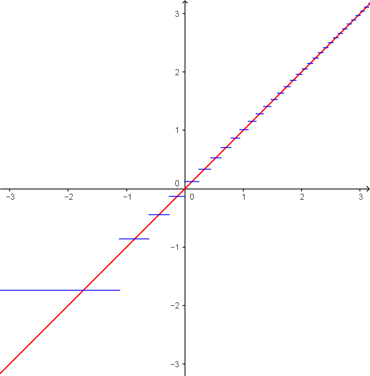
Figure 7: Plot the quantiles of the signed log-likelihood of $Exp^{3.5}$ vs. the quantiles of the signed log-likelihood of $Geo^{3.5}$.

Theorem 6.1

Assume that the random variable $M$ has a geometric distribution $Geo^{\theta}$ and let the random variable $X$ be exponentially distributed $Exp^{\theta}.$ If

$$\Pr\left(X\leq x\right)=\Pr\left(M<m\right)$$

then

$$G_{Geo^{\theta}}\left(m-\nicefrac{{1}}{{2}}\right)\leq G_{Exp^{\theta}}\left(x\right)\leq G_{Geo^{\theta}}\left(m\right)$$

Proof

First we note that $G_{Exp^{\theta}}\left(x\right)=\gamma\left(\nicefrac{{x}}{{\theta}}\right)$ and $\Pr\left(X\leq x\right)=\Pr\left(\nicefrac{{X}}{{\theta}}\leq\nicefrac{{x}}{{\theta}}\right).$ Therefore we introduce the variable $y=\nicefrac{{x}}{{\theta}}$ and the random variable $Y=\nicefrac{{X}}{{\theta}}$ that is exponentially distributed $Exp^{1}.$

We will prove that

$$\Pr\left(Y\leq y\right)=\Pr\left(M<m\right)$$ (2)

implies

$$g_{\theta}\left(m-\nicefrac{{1}}{{2}}\right)\leq\gamma\left(y\right)\leq g_{\theta}\left(m\right).$$

The two inequalities are proved separately.

First we prove that $\Pr\left(Y\leq y\right)=\Pr\left(M<m\right)$ implies that $g_{\theta}\left(m-\nicefrac{{1}}{{2}}\right)\leq\gamma\left(y\right)$. Equivalently we have to prove that

$$\gamma\left(y\right)-g_{\theta}\left(m-\nicefrac{{1}}{{2}}\right)=\frac{\gamma\left(y\right)^{2}-g_{\theta}\left(m-\nicefrac{{1}}{{2}}\right)^{2}}{\gamma\left(y\right)+g_{\theta}\left(m-\nicefrac{{1}}{{2}}\right)}$$

is positive. The probability $\Pr\left(M<m\right)$ is a decreasing function of $\theta.$ Therefore the probability $\Pr\left(Y\leq y\right)$ is a decreasing function of $\theta$, but the destribution of $Y$ does not depend on $\theta$ so $y$ must be a decreasing function of $\theta.$ Therefore the denominator $\gamma\left(y\right)+g_{\theta}\left(m-\nicefrac{{1}}{{2}}\right)$ is a decreasing function of $\theta$ and it equals zero when $\theta=m-\nicefrac{{1}}{{2}}.$ The numerator also equals zero when $\theta=m-\nicefrac{{1}}{{2}}$ so it is sufficient to prove that the numerator is a decreasing function of $\theta.$ Therefore we have to prove the inequality

$$\frac{\partial}{\partial\theta}\left(\gamma\left(y\right)^{2}-g_{\theta}\left(m-\frac{1}{2}\right)^{2}\right)\leq 0$$

or, equivalently, that

$$\frac{\partial}{\partial\theta}\left(g_{\theta}\left(m-\frac{1}{2}\right)^{2}\right)\geq\frac{\partial}{\partial\theta}\left(\gamma\left(y\right)^{2}\right).$$

One also have to prove that $\Pr\left(Y\leq y\right)=\Pr\left(M<m\right)$ implies that $\gamma\left(y\right)\leq g_{\theta}\left(m\right)$ and it is sufficient to prove that

$$\frac{\partial}{\partial\theta}\left(\gamma\left(y\right)^{2}\right)\geq\frac{\partial}{\partial\theta}\left(g_{\theta}\left(m\right)^{2}\right).$$

We have

$$\frac{\partial}{\partial\theta}\left(\gamma\left(y\right)^{2}\right) = \frac{\mathrm{d}y}{\mathrm{d}\theta}\cdot\frac{\mathrm{d}}{\mathrm{d}y}\left(\gamma\left(y\right)^{2}\right)$$

$$= \frac{\mathrm{d}y}{\mathrm{d}\theta}\cdot 2\left(1-\frac{1}{y}\right)\,.$$

For the geometric distribution we have

$$\frac{\partial}{\partial\theta}\left(g_{\theta}\left(m-1\right)^{2}\right) = \frac{\partial}{\partial\theta}\left(2\left(\left(m-1\right)\ln\frac{m-1}{\theta}-m\cdot\ln\frac{m}{\theta+1}\right)\right)$$

$$= 2\left(-\frac{m-1}{\theta}+\frac{m}{\theta+1}\right)$$

$$= 2\frac{\theta-m+1}{\theta+\theta^{2}}\,.$$

Therefore we have to prove that

$$2\frac{\theta-m+\nicefrac{{1}}{{2}}}{\theta+\theta^{2}}\geq 2\frac{\mathrm{d}y}{\mathrm{d}\theta}\cdot\left(1-\frac{1}{y}\right)\geq 2\frac{\theta-m}{\theta+\theta^{2}}\,.$$

Therefore Equation (2) can be solved as

$$1-\exp\left(-y\right) =1-\left(\frac{\theta}{\theta+1}\right)^{m}$$

$$y =m\ln\left(\frac{\theta+1}{\theta}\right).$$

The derivative is

$$\frac{\mathrm{d}y}{\mathrm{d}\theta} =m\left(\frac{1}{\theta+1}-\frac{1}{\theta}\right)$$

$$=-\frac{m}{\theta+\theta^{2}}.$$

Finally we have to prove that

$$\frac{\theta-m+\nicefrac{{1}}{{2}}}{\theta+\theta^{2}} \geq -\frac{m}{\theta+\theta^{2}}\cdot\left(1-\frac{1}{m\ln\left(\frac{\theta+1}{\theta}\right)}\right)\geq\frac{\theta-m}{\theta+\theta^{2}}$$

$$\theta-m+\nicefrac{{1}}{{2}} \geq -m+\frac{1}{\ln\left(\frac{\theta+1}{\theta}\right)}\geq-m+\theta$$

$$\theta+\nicefrac{{1}}{{2}} \geq \frac{1}{\ln\left(\frac{\theta+1}{\theta}\right)}\geq\theta$$

$$\left(\theta+\nicefrac{{1}}{{2}}\right)\ln\left(\frac{\theta+1}{\theta}\right) \geq 1\geq\theta\ln\left(1+\frac{1}{\theta}\right).$$

The right ineqality is trivial. The left inequality is equivalent to

$$\ln\left(\frac{\theta+1}{\theta}\right)-\frac{1}{\theta+\nicefrac{{1}}{{2}}}\geq 0.$$

We have

$$\ln\left(\frac{\theta+1}{\theta}\right)-\frac{1}{\theta+\nicefrac{{1}}{{2}}}\to 0$$

for $\theta\to\infty.$ The derivative is negative

$$\frac{1}{\theta+1}-\frac{1}{\theta}+\frac{1}{\left(\theta+\nicefrac{{1}}{{2}}\right)^{2}}=\frac{-1}{\theta\left(\theta+1\right)\left(2\theta+1\right)^{2}},$$

which proves the theorem.∎

Corollary 1

Assume that the random variable $M$ has a geometric distribution $Geo^{\theta}$ and let the random variable $X$ be exponential distributed $Exp^{\theta}.$ If

$$G_{Exp^{\theta}}\left(x\right)=G_{Geo^{\theta}}\left(m\right)$$

then

$$\Pr\left(M<m\right)\leq\Pr\left(X\leq x\right)\leq\Pr\left(M\leq m\right).$$

If we plot quantiles of an exponential distribution against the corresponding quantiles of the signed log-likelihood of a Geometric distribution we get a stair case function, i.e. a sequence of horisontal lines. The inequality means that the left endpoint of any step is to the left of the line $y=x.$ Actually the line $y=x$ intersects each step and we say that the plot has an intersection property as illustrated in Figure 7.

Proof

Since

$$\Pr\left(X\leq x\right)=\Pr\left(M<m\right)$$

implies

$$G_{Exp^{\theta}}\left(x\right)\leq G_{Geo^{\theta}}\left(m\right)$$

and both $\Pr\left(X\leq x\right)$ and $G_{Exp^{\theta}}\left(x\right)$ are increasing functions of $x$ we have that

$$G_{Exp^{\theta}}\left(x\right)=G_{Geo^{\theta}}\left(m\right)$$

implies that $\Pr\left(X\leq x\right)\geq\Pr\left(M<m\right).$

Since

$$\Pr\left(X\leq x\right)=\Pr\left(M<m\right)$$

implies

$$G_{Geo^{\theta}}\left(m-\nicefrac{{1}}{{2}}\right)\leq G_{Exp^{\theta}}\left(x\right)$$

we have that $G_{Geo^{\theta}}\left(m-\nicefrac{{1}}{{2}}\right)=G_{Exp^{\theta}}\left(x\right)$ implies that $\Pr\left(X\leq x\right)\leq\Pr\left(M<m\right)$. Hence $G_{Geo^{\theta}}\left(m+\nicefrac{{1}}{{2}}\right)=G_{Exp^{\theta}}\left(x\right)$ implies that $\Pr\left(X\leq x\right)\leq\Pr\left(M<m+1\right)=\Pr\left(M\leq m\right).$ Since $G_{Geo^{\theta}}\left(m\right)\leq G_{Geo^{\theta}}\left(m+\nicefrac{{1}}{{2}}\right)$ we also have that $G_{Geo^{\theta}}\left(m\right)=G_{Exp^{\theta}}\left(x\right)$ implies that $\Pr\left(X\leq x\right)\leq\Pr\left(M\leq m\right).$ ∎

7 Inequalities for negative binomial distributions

Compounding a Poisson distribution $Po\left(\lambda\right)$ with rate parameter $\lambda$ distributed according to a Gamma distribution $\Gamma\left(k,\theta\right)$ leads a negative binomial distribution. The link to waiting times in Bernoulli processes will be explored in Sectoin 8. In this section we will parametrize the negative binomial distribution as $neg\left(k,\theta\right)$ where $k$ and $\theta$ are the prameters of the corresponding Gamma distribution. We note that this is an unusual way of parametrizing the negative binomial distribution, but it will be usuful for some of our calculations. Since $\lambda$ is both the mean and the variance of $Po\left(\lambda\right)$ we can calculate the mean of $neg\left(k,\theta\right)$ as $\mu=k\theta$ and the variance as $V$$\left(\mu\right)=\mu+\frac{\mu^{2}}{k}.$

The point probaiblities of a negative binomial distribution can be written in several ways

$$\Pr\left(M=m\right) =\int_{0}^{\infty}\frac{\lambda^{m}}{m!}\exp\left(-\lambda\right)\cdot\frac{1}{\theta^{k}}\frac{1}{\Gamma\left(k\right)}\lambda^{k-1}\exp\left(-\frac{\lambda}{\theta}\right)\,\mathrm{d}\lambda$$

$$=\int_{0}^{\infty}\frac{\left(\theta t\right)^{m}}{m!}\exp\left(-\theta t\right)\cdot\frac{1}{\Gamma\left(k\right)}t^{k-1}\exp\left(-t\right)\,\mathrm{d}t$$

$$=\frac{\Gamma\left(m+k\right)}{m!\Gamma\left(k\right)}\cdot\frac{\theta^{m}}{\left(\theta+1\right)^{m+k}}.$$

We need an explicite formula for the divergence that is given by

$$D\left(\left.neg\left(k,\theta_{1}\right)\right\|neg\left(k,\theta_{2}\right)\right) =\int_{k\theta_{1}}^{k\theta_{2}}\frac{\mu-k\theta_{1}}{\mu+\frac{\mu^{2}}{k}}\,\mathrm{d}\mu$$

$$=k\left(\theta_{1}\ln\frac{\theta_{1}}{\theta_{2}}-\left(\theta_{1}+1\right)\ln\frac{\theta_{1}+1}{\theta_{2}+1}\right).$$

The log-likelihood is given by

$$G_{neg\left(k,\theta\right)}\left(x\right) =k^{\nicefrac{{1}}{{2}}}g_{\theta}\left(\frac{x}{k}\right)$$

where $g_{\theta}$ is given by Equation 1.

We will need the following lemma.

Lemma 7

A Poisson random variable $K$ with distribution $Po\left(\lambda\right)$ satisfies

$$\frac{\mathrm{d}}{\mathrm{d}\lambda}\Pr\left(K\leq k\right)=-\Pr\left(K=k\right).$$

Proof

If $X$ is a Gamma distributed $\Gamma\left(k+1,1\right)$ then

$$\Pr\left(K\leq k\right) =\Pr\left(K<k+1\right)$$

$$=1-\Pr\left(X\leq\lambda\right).$$

Hence

$$\frac{\mathrm{d}}{\mathrm{d}\lambda}\Pr\left(K\leq k\right) =-\frac{1}{1^{k}}\frac{1}{\Gamma\left(k+1\right)}\lambda^{\left(k+1\right)-1}\exp\left(-\frac{\lambda}{1}\right)$$

$$=-\frac{\lambda^{k}}{k!}\exp\left(-\lambda\right),$$

which proves the lemma.∎

Lemma 8

If the distribution of $M_{k}$ is $neg\left(k,\theta\right)$ then the partial derivative of the point probability with respect to the mean value parameter equals

$$\frac{\mathrm{d}}{\mathrm{d}\mu}\Pr\left(M_{k}\leq m\right)=-\Pr\left(M_{k+1}=m\right).$$

where $M_{k+1}$ is $neg\left(k+1,\theta\right).$

Proof

We have

$$\frac{\mathrm{d}}{\mathrm{d}\mu}\Pr\left(M_{k}\leq m\right) =\frac{1}{\frac{\mathrm{d}\mu}{\mathrm{d}\theta}}\cdot\frac{\mathrm{d}}{\mathrm{d}\theta}\left(\int_{0}^{\infty}\left(\sum_{j=0}^{m}Po\left(\theta t;j\right)\right)\cdot\frac{1}{\Gamma\left(k\right)}t^{k-1}\exp\left(-t\right)\,\mathrm{d}t\right)$$

$$=\frac{1}{k}\cdot\int_{0}^{\infty}\left(-t\cdot Po\left(\theta t;m\right)\right)\cdot\frac{1}{\Gamma\left(k\right)}t^{k-1}\exp\left(-t\right)\,\mathrm{d}t$$

$$=-\int_{0}^{\infty}Po\left(\theta t;m\right)\cdot\frac{1}{\Gamma\left(k+1\right)}t^{k}\exp\left(-t\right)\,\mathrm{d}t.$$

The last integral equals $-\Pr\left(M_{k+1}=m\right),$ which proves the lemma. ∎

The following theorem generalizes Corollary 1 from $k=1$ to arbitrary positive values of $k.$ We cannot use the same proof technique because we do not have an explicite formula for the quantile function for the Gamma distributions except in the case when $k=1.$ Lemma 4 cannot be used because we want to compare a discrete distribution with a continuous function. Instead the proof combines a proof method developed by Zubkov and Serov Zubkov and Serov (2013) with the ideas and results developed in the previous sections.

Theorem 7.1

Assume that the random variable $M$ has a negative binomial distribution $neg\left(k,\theta\right)$ and let the random variable $X$ be Gamma distributed $\Gamma\left(k,\theta\right).$ If

$$G_{\Gamma\left(k,\theta\right)}\left(x\right)=G_{neg\left(k,\theta\right)}\left(m\right)$$

then

$$\Pr\left(M<m\right)\leq\Pr\left(X\leq x\right)\leq\Pr\left(M\leq m\right).$$ (3)

Proof

Below we only give the proof of the upper bound in Inequality 3. The lower bound is proved the in the same way.

First we note that $G_{\Gamma\left(k,\theta\right)}\left(x\right)=G_{\Gamma\left(k,1\right)}\left(\nicefrac{{x}}{{\theta}}\right)$ and

$$\Pr\left(X\leq x\right)=\Pr\left(\nicefrac{{X}}{{\theta}}\leq\nicefrac{{x}}{{\theta}}\right).$$

Therefore we introduce the variable $y=\nicefrac{{x}}{{\theta}}$ and the random variable $Y=\nicefrac{{X}}{{\theta}}$ that is Gamma distributed $\Gamma\left(k,1\right).$ Introduce the difference

$$\delta\left(\mu_{0}\right)=\Pr\left(M\leq m\right)-\Pr\left(Y\leq y\right)$$

and note that

$$\delta\left(0\right)=\lim_{\mu_{0}\to\infty}\delta\left(\mu_{0}\right)=0.$$ (4)

We note that there exists (at least) one value of $\mu_{0}$ such that $\frac{\partial\delta}{\partial\mu_{0}}=0.$ It is sufficient to prove that $\delta$ is first increasing and then decreasing in $\left[0,\infty\right[.$

According to Lemma 8 the derivative of $\Pr\left(M\leq m\right)$ with respect to $\mu_{0}$ is

$$\frac{\partial}{\partial\mu_{0}}\Pr\left(M\leq m\right) =-\frac{\Gamma\left(m+k+1\right)}{m!\Gamma\left(k+1\right)}\cdot\frac{\theta^{m}}{\left(\theta+1\right)^{m+k+1}}.$$

$$=-\frac{m+k}{k\left(\theta+1\right)}\frac{\Gamma\left(m+k\right)}{m!\Gamma\left(k\right)}\cdot\frac{\theta^{m}}{\left(\theta+1\right)^{m+k}}$$

$$=-\frac{m+k}{\mu_{0}+k}\Pr\left(M=m\right)$$

$$=-\frac{\hat{\theta}+1}{\theta+1}\Pr\left(M=m\right)$$

where $\theta=\mu_{0}/k$ is the scale parameter and where and $\hat{\theta}=\nicefrac{{m}}{{k}}$ is the maximum likelihood estimate of the scale parameter. Let $\hat{\Pr}$ denote the probability of $M$ calculated with respect to this maximum likelihood estimate $\hat{\theta}$. Then we have

$$\frac{\partial}{\partial\theta}\Pr\left(M\leq m\right) =-\frac{m+k}{\theta+1}\exp\left(-D\right)\hat{\Pr}\left(M=m\right).$$

The condition

$$G_{\Gamma\left(k,\theta\right)}\left(x\right)=G_{neg\left(k,\theta\right)}\left(m\right)$$

can be written as

$$k^{\nicefrac{{1}}{{2}}}\gamma\left(\frac{y}{k}\right)=k^{\nicefrac{{1}}{{2}}}g_{\theta}\left(\hat{\theta}\right)$$

which implies

$$\left(\gamma\left(\frac{y}{k}\right)\right)^{2}=\left(g_{\theta}\left(\hat{\theta}\right)\right)^{2}.$$

Differentiation with respect to $\theta$ gives

$$2\left(1-\frac{k}{y}\right)\frac{1}{k}\frac{dy}{d\theta}=2\frac{\theta-\hat{\theta}}{\theta+\theta^{2}}$$

so that

$$\frac{dy}{d\theta}=\frac{1}{\frac{1}{k}-\frac{1}{y}}\cdot\frac{\theta-\hat{\theta}}{\theta+\theta^{2}}$$

Therefore

$$\frac{\partial}{\partial\theta}\Pr\left(Y\leq y\right) =f\left(y\right)\cdot\frac{dy}{d\theta}$$

$$=\frac{k^{k}\tau^{\nicefrac{{1}}{{2}}}\exp\left(-k\right)}{\Gamma\left(k\right)k^{\nicefrac{{1}}{{2}}}}\cdot\frac{\exp\left(-D\right)}{y}\cdot\frac{1}{\frac{1}{k}-\frac{1}{y}}\cdot\frac{\theta-\hat{\theta}}{\theta+\theta^{2}}$$

$$=\frac{k^{k}\tau^{\nicefrac{{1}}{{2}}}\exp\left(-k\right)}{\Gamma\left(k\right)k^{\nicefrac{{1}}{{2}}}}\cdot\frac{\exp\left(-D\right)}{\frac{y}{k}-1}\cdot\frac{\theta-\hat{\theta}}{\theta+\theta^{2}}$$

$$=\frac{k^{k}\tau^{\nicefrac{{1}}{{2}}}\exp\left(-k\right)}{\Gamma\left(k\right)k^{\nicefrac{{1}}{{2}}}}\cdot\frac{\exp\left(-D\right)}{\gamma^{-1}\left(g_{\theta}\left(\hat{\theta}\right)\right)-1}\cdot\frac{\theta-\hat{\theta}}{\theta\left(\theta+1\right)}$$

Combining these results we get

$$\frac{\partial\delta}{\partial\theta}=-\frac{m+k}{\theta+1}\hat{\Pr}\left(M=m\right)\cdot\exp\left(-D\right)\\ -\frac{k^{k}\tau^{\nicefrac{{1}}{{2}}}\exp\left(-k\right)}{\Gamma\left(k\right)k^{\nicefrac{{1}}{{2}}}}\cdot\frac{\exp\left(-D\right)}{\left(\gamma^{-1}\left(g_{\theta}\left(\hat{\theta}\right)\right)-1\right)}\cdot\frac{\theta-\hat{\theta}}{\theta\left(1+\theta\right)}\\ =\frac{k^{k}\tau^{\nicefrac{{1}}{{2}}}\exp\left(-k\right)}{\Gamma\left(k\right)}\cdot\frac{\exp\left(-D\right)}{\theta+1}\cdot\\ \left(\frac{\hat{\theta}-\theta}{\theta\cdot\left(\gamma^{-1}\left(g_{\theta}\left(\hat{\theta}\right)\right)-1\right)}-\frac{\Gamma\left(k\right)\left(m+k\right)}{k^{k}\tau^{\nicefrac{{1}}{{2}}}\exp\left(-k\right)}\cdot\hat{\Pr}\left(M=m\right)\right).$$

Remark that the first factor is positive and that

$$\frac{\Gamma\left(k\right)k^{\nicefrac{{1}}{{2}}}}{k^{k}\tau^{\nicefrac{{1}}{{2}}}\exp\left(-k\right)}\cdot k\left(\hat{\theta}+1\right)\cdot\hat{\Pr}\left(M=m\right)$$

is a positive number that does not depend on $\theta.$ Therefore it is sufficient to prove that $\frac{\hat{\theta}-\theta}{\theta\cdot\left(\gamma^{-1}\left(g_{\theta}\left(\hat{\theta}\right)\right)-1\right)}$ is a decreasing function of $\theta$, or, equivalently, to prove that $\frac{\theta\cdot\gamma^{-1}\left(g_{\theta}\left(\hat{\theta}\right)\right)-\theta}{\hat{\theta}-\theta}$ is an increasing function of $\theta.$

The partial derivative with respect to $\theta$ is

$$\frac{\left(\hat{\theta}-\theta\right)\left(\gamma^{-1}\left(g_{\theta}\left(\hat{\theta}\right)\right)+\frac{\theta\cdot\gamma^{-1}\left(g_{\theta}\left(\hat{\theta}\right)\right)}{\gamma^{-1}\left(g_{\theta}\left(\hat{\theta}\right)\right)-1}\cdot\frac{\theta-\hat{\theta}}{\theta+\theta^{2}}-1\right)+\theta\cdot\gamma^{-1}\left(g_{\theta}\left(\hat{\theta}\right)\right)-\theta}{\left(\hat{\theta}-\theta\right)^{2}}\\ =\frac{\frac{\gamma^{-1}\left(g_{\theta}\left(\hat{\theta}\right)\right)-1}{\gamma^{-1}\left(g_{\theta}\left(\hat{\theta}\right)\right)}-\frac{\left(\hat{\theta}-\theta\right)^{2}}{\hat{\theta}\left(1+\theta\right)\left(\gamma^{-1}\left(g_{\theta}\left(\hat{\theta}\right)\right)-1\right)}}{\frac{\left(\hat{\theta}-\theta\right)^{2}}{\hat{\theta}\cdot\gamma^{-1}\left(g_{\theta}\left(\hat{\theta}\right)\right)}}\,.$$

We have to prove that

$$\frac{\gamma^{-1}\left(g_{\theta}\left(\hat{\theta}\right)\right)-1}{\gamma^{-1}\left(g_{\theta}\left(\hat{\theta}\right)\right)} \geq\frac{\left(\hat{\theta}-\theta\right)^{2}}{\hat{\theta}\left(1+\theta\right)\left(\gamma^{-1}\left(g_{\theta}\left(\hat{\theta}\right)\right)-1\right)}\,.$$

If $\hat{\theta}\geq\theta$ the inequality is equivalent to

$$\frac{\left(\gamma^{-1}\left(g_{\theta}\left(\hat{\theta}\right)\right)-1\right)^{2}}{\gamma^{-1}\left(g_{\theta}\left(\hat{\theta}\right)\right)}\geq\frac{\left(\hat{\theta}-\theta\right)^{2}}{\hat{\theta}\left(1+\theta\right)}$$

If $\hat{\theta}<\theta$ the inequality is equivalent to

$$\frac{\left(\gamma^{-1}\left(g_{\theta}\left(\hat{\theta}\right)\right)-1\right)^{2}}{\gamma^{-1}\left(g_{\theta}\left(\hat{\theta}\right)\right)}\leq\frac{\left(\hat{\theta}-\theta\right)^{2}}{\hat{\theta}\left(1+\theta\right)}$$

The equation $\frac{\left(s-1\right)^{2}}{s}=t$ can be solved with respect to $x$, which gives the solutions $s=1+\frac{t}{2}\pm\frac{\left[t^{2}+4t\right]^{\nicefrac{{1}}{{2}}}}{2}.$ For $\hat{\theta}\geq\theta$ we get

$$\gamma^{-1}\left(g_{\theta}\left(\hat{\theta}\right)\right) \geq 1+\frac{\frac{\left(\hat{\theta}-\theta\right)^{2}}{\hat{\theta}\left(1+\theta\right)}}{2}+\frac{\left[\left(\frac{\left(\hat{\theta}-\theta\right)^{2}}{\hat{\theta}\left(1+\theta\right)}\right)^{2}+4\frac{\left(\hat{\theta}-\theta\right)^{2}}{\hat{\theta}\left(1+\theta\right)}\right]^{\nicefrac{{1}}{{2}}}}{2}$$

$$=1+\left(\hat{\theta}-\theta\right)\frac{\hat{\theta}-\theta+\left[\left(\hat{\theta}+\theta\right)^{2}+4\hat{\theta}\right]^{\nicefrac{{1}}{{2}}}}{2\hat{\theta}\left(1+\theta\right)}$$

For $\hat{\theta}<\theta$ we get

$$\gamma^{-1}\left(g_{\theta}\left(\hat{\theta}\right)\right) \geq 1+\frac{\frac{\left(\hat{\theta}-\theta\right)^{2}}{\hat{\theta}\left(1+\theta\right)}}{2}-\frac{\left[\left(\frac{\left(\hat{\theta}-\theta\right)^{2}}{\hat{\theta}\left(1+\theta\right)}\right)^{2}+4\frac{\left(\hat{\theta}-\theta\right)^{2}}{\hat{\theta}\left(1+\theta\right)}\right]^{\nicefrac{{1}}{{2}}}}{2}$$

$$=1+\left(\hat{\theta}-\theta\right)\frac{\hat{\theta}-\theta+\left[\left(\hat{\theta}+\theta\right)^{2}+4\hat{\theta}\right]^{\nicefrac{{1}}{{2}}}}{2\hat{\theta}\left(1+\theta\right)}$$

Since $\gamma$ is increasing we have to prove that

$$g_{\theta}\left(\hat{\theta}\right)\geq\gamma\left(1+\left(\hat{\theta}-\theta\right)\frac{\hat{\theta}-\theta+\left[\left(\hat{\theta}+\theta\right)^{2}+4\hat{\theta}\right]^{\nicefrac{{1}}{{2}}}}{2\hat{\theta}\left(1+\theta\right)}\right)$$

or, equivalently, that

$$g_{\theta}\left(\hat{\theta}\right)-\gamma\left(1+\left(\hat{\theta}-\theta\right)\frac{\hat{\theta}-\theta+\left[\left(\hat{\theta}+\theta\right)^{2}+4\hat{\theta}\right]^{\nicefrac{{1}}{{2}}}}{2\hat{\theta}\left(1+\theta\right)}\right)\\ =\frac{\left\{g_{\theta}\left(\hat{\theta}\right)\right\}^{2}-\left\{\gamma\left(1+\left(\hat{\theta}-\theta\right)\frac{\hat{\theta}-\theta+\left[\left(\hat{\theta}+\theta\right)^{2}+4\hat{\theta}\right]^{\nicefrac{{1}}{{2}}}}{2\hat{\theta}\left(1+\theta\right)}\right)\right\}^{2}}{g_{\theta}\left(\hat{\theta}\right)+\gamma\left(1+\left(\hat{\theta}-\theta\right)\frac{\hat{\theta}-\theta+\left[\left(\hat{\theta}+\theta\right)^{2}+4\hat{\theta}\right]^{\nicefrac{{1}}{{2}}}}{2\hat{\theta}\left(1+\theta\right)}\right)}$$

is positive. Both the denominator and the numerator are zero when $\theta=\hat{\theta}.$ Therefore it is sufficient to prove that both the denominator and the numerator are decreasing functions of $\theta.$

First we prove that the denominator is decreasing. The first term is obviously decreasing. The second term is composed of $\gamma$, which is increasing, and $y\curvearrowright 1+\frac{y}{2}\pm\frac{\left[y^{2}+4y\right]^{\nicefrac{{1}}{{2}}}}{2}$ which is increasing or decreasing depending on the sign of $\pm,$ and the function $\theta\curvearrowright\frac{\left(\hat{\theta}-\theta\right)^{2}}{\hat{\theta}\left(1+\theta\right)}$ which is decreasing when $\theta\leq\hat{\theta}$ and increasing when $\theta\geq\hat{\theta}.$ Therefore the composed function is a decreasing function of $\theta.$

The numerator can be written as

$$2\left\{\hat{\theta}\ln\frac{\hat{\theta}}{\theta}-\left(\hat{\theta}+1\right)\ln\frac{\hat{\theta}+1}{\theta+1}\right\}-2\left\{\begin{array}[]{c}\left(\hat{\theta}-\theta\right)\frac{\hat{\theta}-\theta+\left[\left(\hat{\theta}+\theta\right)^{2}+4\hat{\theta}\right]^{\nicefrac{{1}}{{2}}}}{2\hat{\theta}\left(1+\theta\right)}\\ -\ln\left(1+\left(\hat{\theta}-\theta\right)\frac{\hat{\theta}-\theta+\left[\left(\hat{\theta}+\theta\right)^{2}+4\hat{\theta}\right]^{\nicefrac{{1}}{{2}}}}{2\hat{\theta}\left(1+\theta\right)}\right)\end{array}\right\}.$$

We calculate the derivative with respect to $\theta$, which can be written as

$$\frac{-4\frac{2\theta+\hat{\theta}+4}{\theta+\theta^{2}}\left(\theta-\hat{\theta}\right)^{2}}{\theta\left(\theta+\hat{\theta}+2\right)\left[\left(\hat{\theta}+\theta\right)^{2}+4\hat{\theta}\right]^{\nicefrac{{1}}{{2}}}+\left(\theta+2\right)\left(\left(\hat{\theta}+\theta\right)^{2}+4\hat{\theta}\right)},$$

which is obviously less than or equal to zero. ∎

If we want to give lower bounds and upper bounds to the tail probabilities of a negative binomial distribution the following reformulation of Theorem 7.1 is useful.

Corollary 2

Assume that the random variable $M$ has a negative binomial distribution $neg\left(k,\theta\right)$ and let the random variable $X$ be Gamma distributed $\Gamma\left(k,\theta\right).$ If

$$G_{\Gamma\left(k,\theta\right)}\left(x\right)=G_{neg\left(k,\theta\right)}\left(m\right)$$

Then

$$\Pr\left(X\leq x_{m}\right)\leq\Pr\left(M\leq m\right)\leq\Pr\left(X\leq x_{m+1}\right)$$ (5)

where $x_{m}$ and $x_{m+1}$ are determined by

$$G_{\Gamma\left(k,\theta\right)}\left(x_{m}\right) =G_{neg\left(k,\theta\right)}\left(m\right),$$

$$G_{\Gamma\left(k,\theta\right)}\left(x_{m+1}\right) =G_{neg\left(k,\theta\right)}\left(m+1\right).$$

8 Inequalities for binomial distributions and Poisson distributions

We will prove that intersections results for binomial distributions and Poisson distributions follows from the corresponding intersection result for negative binomial distributions and Gamma distributions. We note that the point probabilities of a negative binomial distribution can be written as

$$\frac{\Gamma\left(m+k\right)}{m!\Gamma\left(k\right)}\cdot\frac{\theta^{m}}{\left(\theta+1\right)^{m+k}}=\frac{k^{\bar{m}}}{m!}p^{k}\left(1-p\right)^{m}$$

where $p=\frac{1}{1+\theta}$ and where $\bar{m}$ denotes the raising factorial. Let $nb\left(p,k\right)$ denote a negativ binomial distribution with succes probability $p$. Then $nb\left(p,k\right)$ is the distribution of the number of failures before the $k$’th success in a Bernoulli process with success probability $p.$

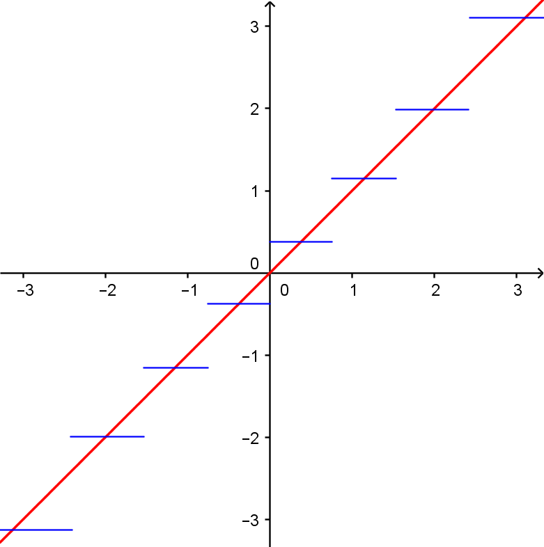
Figure 8: Plot the quantiles of the signed log-likelihood of a standard Gaussian vs. the quantiles of the sigend log-likelihood of $bin\left(7,\nicefrac{{1}}{{2}}\right)$.

Our inequality for the negative binomial distribution can be translated into an inequality for the binomial distribution. Assume that $K$ is binomial $bin\left(n,p\right)$ and $M$ is negative binomial $nb\left(p,k\right).$ Then

$$\Pr\left(K\geq k\right)=\Pr\left(M+k\leq n\right).$$

In terms of $p$ the divergence can be written as

$$D\left(\left.nb\left(p_{1},k\right)\right\|nb\left(p_{2},k\right)\right) =\frac{k}{p_{1}}\left(p_{1}\ln\frac{p_{1}}{p_{2}}+\left(1-p_{1}\right)\ln\frac{1-p_{1}}{1-p_{2}}\right).$$

We have

$$D\left(\left.bin\left(n,p_{1}\right)\right\|bin\left(n,p_{2}\right)\right)=p_{1}\ln\frac{p_{1}}{p_{2}}+\left(1-p_{1}\right)\ln\frac{1-p_{1}}{1-p_{2}}$$

so

$$D\left(\left.nb\left(\frac{k}{n},k\right)\right\|nb\left(p,k\right)\right) =n\left(\frac{k}{n}\ln\frac{\frac{k}{n}}{p_{2}}+\left(1-\frac{k}{n}\right)\ln\frac{1-\frac{k}{n}}{1-p_{2}}\right)$$

$$=D\left(\left.bin\left(n,\frac{k}{n}\right)\right\|bin\left(n,p\right)\right).$$

If $G_{bin}$ is the signed log-likelihood of $bin\left(n,p\right)$ and $G_{nb}$ is the signed log-likelihood of $nb\left(p,k\right)$ then $G_{bin\left(n,p\right)}\left(k\right)=-G_{nb\left(p,k\right)}\left(n-k\right).$

If $K$ is Poisson distributed with mean $\lambda$ and $X$ is Gamma distributed with shape parameter $k$ and scale parameter 1, i.e. the distribution of the waiting time until $k$ observations from an Poisson process with intensity 1. Then

$$\Pr\left(K\geq k\right)=\Pr\left(X\leq\lambda\right).$$

Next we note that

$$D\left(Po\left(k\right)\|Po\left(\lambda\right)\right)=D\left(\left.\Gamma\left(k,\frac{\lambda}{k}\right)\right\|\Gamma\left(k,1\right)\right).$$

If $G_{Po\left(\lambda\right)}$ is the signed log-likelihood for $Po\left(\lambda\right)$ and $G_{\Gamma\left(k,1\right)}$ is the signed log-likelihood for $\Gamma\left(k,1\right)$ then $G_{Po\left(\lambda\right)}\left(k\right)=-G_{\Gamma\left(k,1\right)}\left(\lambda\right).$

Theorem 8.1

Assume that $K$ is binomially distributed $bin\left(n,p\right)$ and let $G_{bin\left(n,p\right)}$ denote the signed log-likelihood function of the exponential family based on $bin\left(n,p\right).$ Assume that $L$ is a Poisson random variable with distribution $Po\left(\lambda\right)$ and let $G_{Po\left(\lambda\right)}$ denote the signed log-likelihood function of the exponential family based on $Po\left(\lambda\right).$ If

$$G_{bin\left(n,p\right)}\left(k\right)=G_{Po\left(\lambda\right)}\left(k\right)$$

Then

$$\Pr\left(K<k\right)\leq\Pr\left(L<k\right)\leq\Pr\left(K\leq k\right).$$ (6)

Proof

Let $M$ denote a negative binomial random variable with distribution $nb\left(p,k\right)$ and let $X$ denote a Gamma random variable with distribution $\Gamma\left(k,\theta\right)$ where the parameter $\theta$ equals $\frac{1}{p}-1$ such that the distributions $nb\left(p,k\right)$ and $\Gamma\left(k,\theta\right)$ have the same mean value. Now $G_{nb\left(p,k\right)}\left(n-k\right)=-G_{bin\left(n,p\right)}\left(k\right)$ and $G_{\Gamma\left(k,\theta\right)}\left(\lambda\theta\right)=-G_{Po\left(\lambda\right)}\left(k\right).$ Then $G_{nb\left(p,k\right)}\left(n-k\right)=G_{\Gamma\left(k,\theta\right)}\left(\lambda\theta\right).$ The left part of the Inequality 6 is proved as follows.

$$\Pr\left(K<k\right) =1-\Pr\left(K\geq k\right)$$

$$=1-\Pr\left(M+k\leq n\right)$$

$$\leq 1-\Pr\left(X\leq\lambda\theta\right)$$

$$=1-\Pr\left(L\geq k\right)$$

$$=\Pr\left(L<k\right).$$

The right part of the inequality is proved in the same way. ∎

Note that Theorem 7.1 cannot be proved from Theorem 8.1 because the number parameter for a binomial distribution has to be an integer while the number parameter of a negative binomial distribution may assume any positive value. Now, our inequalities for negative binomial distributions can be translated into inequalities for binomial distributions.

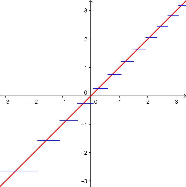
Figure 9: Plot of quantiles of a standard Gaussian vs. the log-ligelihood of the Poisson distribution $Po\left(3.5\right).$

Now we can prove the an intersection inequalities for the binomial family as stated in the following theorem that was recently proved by Serov and Zubkov Zubkov and Serov (2013).

Corollary 3

Assume that $K$ is binomially distributed $bin\left(n,p\right)$ and let $G_{bin\left(n,p\right)}$ denote the signed log-likelihood function of the exponential family based on $bin\left(n,p\right).$ Then

$$\Pr\left(K<k\right)\leq\Phi\left(G_{bin\left(n,p\right)}\left(k\right)\right)\leq\Pr\left(K\leq k\right).$$ (7)

Similarly, assume that $L$ is Poisson distributed $Po\left(\lambda\right)$ and let $G_{Po\left(\lambda\right)}$ denote the signed log-likelihood function of the exponential family based on $Po\left(\lambda\right).$ Then

$$\Pr\left(L<k\right)\leq\Phi\left(G_{Po\left(\lambda\right)}\left(k\right)\right)\leq\Pr\left(L\leq k\right).$$ (8)

Proof

First we prove the left part of Inequality (8). Let $X$ denote a Gamma distributed $\Gamma\left(k,1\right)$ and let $Z$ denote a standard Gaussian. Then $G_{Po\left(\lambda\right)}\left(k\right)=-G_{\Gamma\left(k,1\right)}\left(\lambda\right)$ and

$$\Pr\left(L<k\right) =1-\Pr\left(L\geq k\right)$$

$$=1-\Pr\left(X\leq\lambda\right)$$

$$=\Pr\left(X\geq\lambda\right)$$

$$\leq\Pr\left(Z\geq G_{\Gamma\left(k,1\right)}\left(\lambda\right)\right)$$

$$=\Pr\left(Z\geq-G_{Po\left(\lambda\right)}\left(k\right)\right)$$

$$=\Phi\left(G_{Po\left(\lambda\right)}\left(k\right)\right).$$

The left part of Inequality (7) is obtained by combining the left part of Inequality (8) with the left part of Inequality (6).∎

Proof

The right part of Inequality (7) is obtained follows from the left part of Inequality (7) by replacing $p$ by $1-p$ and replacing $k$ by $n-k.$

Proof

Since a Poisson distribution is a limit of binomial distributions the right part of Inequality (8) follows from the right part of Inequality (8). ∎

The intersection property for Poisson distributions was proved in Harremoës and Tusnády (2012) where the inequality for binomial distributions was also conjectured.

9 Summary

The main theorems in this paper are domination theorems and intersection theorems. The first type of inequalities states that the signed log-likelihood of one distribution is dominated by the signed loglikelihood of another distribution, i.e. the distribution function of the first distribution is larger than the distribution function of the second distribution.

signed ll	dom. by signed ll	Condition	Theorem
Inverse Gaussian	Gaussian		3.1
$IG\left(\mu_{1},\lambda_{1}\right)$	$IG\left(\mu_{2},\lambda_{2}\right)$	$\frac{\mu_{1}}{\lambda_{1}}>\frac{\mu_{2}}{\lambda_{2}}$	3.2
Gamma	Gaussian		5.1
$\Gamma_{k_{1},\theta_{1}}$	$\Gamma_{k_{2},\theta_{2}}$	$k_{1}\leq k_{2}$	5.2

Table 1: Stochastic domination results. Note that the exponential distributions are special cases of Gamma distributions.

The second type of result are intersection results, i.e. the distribution function of the log-likelihood of a discrete distribution is a staircase function where each step is intersected by the distribution function of the log-likelihood of a continuous distribution.

Discrete distribution	Continuous distribution	Theorem
Geometric	Exponential	1
Negative binomial	Gamma	7.1
Binomial	Gaussian	3
Poisson	Gaussian	3

Table 2: Intersection results.

10 Discussion

In this paper we have presented inequalities of two types. The inequalities for inverse Gaussian distributions, exponential distributions and other Gamma distributions are about stochastic domination. The inequalities for Poisson distributions, binomial distributions, geometric distributions and other negative binomial distributions are about intersection. These inequalities can be combined in order to get inequalities of other types. For instance a negative binomial random variable $M$ with distribution $neg\left(k,\theta\right)$ satisfies

$$\Phi\left(G_{neg\left(k,\theta\right)}\left(m\right)\right)\leq\Pr\left(M\leq m\right),$$

where $G_{nb\left(p,k\right)}$ denotes the signed log-likelihood of the negative binomial distribution. Contrary to the similar inequality for the binomial distribution the inquality $\Pr\left(M<m\right)\leq\Phi\left(G_{neg\left(k,\theta\right)}\left(m\right)\right)$ does in general not hold as illustrated in Figure 10.

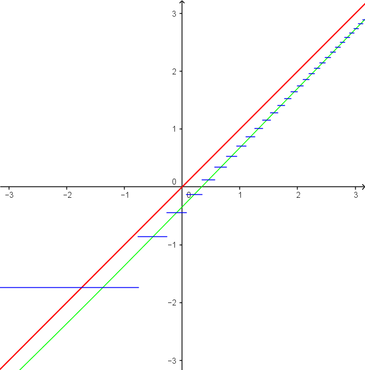
Figure 10: Plot of the quantiles of a standard Gaussian vs. the quantiles of the signed log-likelihood of the negative binomial distribution $neg\left(1,3.5\right)$ (blue) and of the signed log-likelihood of the Gamma distribution $\Gamma\left(1,3.5\right)$ (green).

We have both lower bounds and upper bounds on the Poission distributions. The upper bound for the Poisson distribution corresponds to the lower bound for the Gamma distribution presented in Theorem 5.1, but the lower for the Poisson distribution translated into a new upper bound for the distribution function of the Gamma distribution. Numerical calculations also indicates that in Inequality (8) the right hand inequality can be improved to

$$\Phi\left(G_{Po\left(\lambda\right)}\left(k+\frac{1}{2}\right)\right)\leq\Pr\left(L\leq k\right).$$

This inequality is much tighter than the inequality in (8). Similarly, J. Reiczigel, L. Rejtő and G. Tusnády conjectured that both the lower bound and the upper bound in Inequality 7 can be significantly improved when for $p=\nicefrac{{1}}{{2}}$ Reiczigel et al (2011), and their conjecture has been a major motivation for initializing this research.

For the most important distributions like the binomial distributions, the Poisson distributions, the negative binomial distributions, the inverse Gaussian distributions and the Gamma distributions we can formulate sharp inequalities that hold for any sample size. All these distributions have variance functions that are polynomials of order 2 and 3. Natural exponential families with polynomial variance functions of order at most 3 have been classified Morris (1982); Letac and Mora (1990) and there is a chance that one can formulate and prove sharp inequalities for each of these exponential families. Although there may exist very nice results for the rest of the exponential families with simple variance functions the rest of these exponential families have much fewer applications than the exponential families that have been the subject of the present paper.

In the present paper inequalities have been developed for specific exponential families, but one may hope that some more general inequalities may be developed where bounds on the tails are derived directly from the properties of the variace function.