Angular momentum fluxes caused by $\Lambda$-effect and meridional circulation structure of the Sun

Abstract

Using mean-field hydrodynamic models of the solar angular momentum balance we show that the non-monotonic latitudinal dependence of the radial angular momentum fluxes caused by $\Lambda$-effect can affect the number of the meridional circulation cells stacking in radial direction in the solar convection zone. In particular, our results show the possibility of a complicated triple-cell meridional circulation structure. This pattern consists of two large counterclockwise circulation cells (the N-hemisphere) and a smaller clockwise cell located at low latitudes at the bottom of the convection zone.

1 Introduction

The mean-field models have been successful in explaining basic properties of the differential rotation of the Sun and solar-like stars, e.g., Küker & Rüdiger (2005) and Kitchatinov & Olemskoy (2011). These models predicted dependence of the the surface latitudinal shear on the rotation rate and the spectral class for a set of low-main-sequence solar-like stars with external convection zone, (Kitchatinov & Rüdiger, 1999). However, recent findings from analysis of the supergranulation dynamics on the Sun (Hathaway, 2012) and helioseismology inversions (Zhao et al., 2013; Kholikov et al., 2014) put in question the results of the mean-field models predicting a single-cell meridional circulation structure of the solar convection zone. Global 3D simulations of the flows in the solar convection zone also show the multiple-cell structure of the meridional circulation (Käpylä et al., 2011; Miesch et al., 2011; Guerrero et al., 2013).

In this note we show that the double-cell meridional circulation structure can be compatible with the solar-like rotation law in the framework of the mean-field theory. The $\Lambda$-effect is one of the key ingredient of the mean-field models of solar differential rotation It is caused by effect of the Coriolis forces on convective flows the stratified rotating convection zones (Kichatinov & Rudiger, 1993). The $\Lambda$-effect produces non-disspative angular momentum fluxes. Therefore the spatial structure of the $\Lambda$-effect determine the spatial structure of the global flows in the stellar convection zone. For example, the latitudinal dependence of the $\Lambda$-effect determines the radial profile of the angular velocity distribution (Kichatinov & Rudiger, 1993). Here, we study how it affects the structure of the meridional circulation. The study is carried out using the standard mean-field models of the angular momentum balance and heat transport in the solar convection zone.

2 Basic equations

The reference internal thermodynamic structure of the Sun is calculated using the MESA stellar evolution code (version r7623) (Paxton et al., 2011, 2013). The model is calculated using the mixing length parameter $\alpha_{MLT}={\displaystyle\frac{\ell}{H_{p}}}=2$, where $H_{p}$ is the pressure scale.

2.1 Heat transport

Following to Kitchatinov & Rüdiger (1999), effects of rotation on the thermal balance are calculated from the mean-field heat transport equation,

$$\overline{\rho}\overline{T}\frac{\partial s}{\partial t}+\overline{\rho}\overline{T}\left(\overline{\mathbf{U}}\cdot\boldsymbol{\nabla}\right)s=-\boldsymbol{\nabla}\cdot\left(\mathbf{F}^{conv}+\mathbf{F}^{rad}\right),$$ (1)

where $\mathbf{\overline{U}}$ is axisymmetric mean flow. We employ the expression for the anisotropic convective flux suggested by Kichatinov et al. (1994),

$$F_{i}^{conv}=\overline{\rho}\overline{T}\chi_{ij}\nabla_{j}s,$$ (2)

where the heat conductivity tensor $\chi_{ij}$ reads

$$\chi_{ij}=\chi_{T}\left(\phi\left(\Omega^{*}\right)+c_{\chi}\phi_{\parallel}\left(\Omega^{*}\right)\frac{\Omega_{i}\Omega_{j}}{\Omega^{2}}\right).$$

Functions $\phi$, $\phi_{\parallel}$ are defined in the above cited paper. The effect of the global rotation on the heat transport depends on the Coriolis number $\Omega^{*}=2\tau_{c}\Omega_{0}$, where $\tau_{c}$ is the turn-over time of convective flow. Following to Kitchatinov & Olemskoy (2011) we assume $c_{\chi}=1.5$. If we neglect rotation ($\Omega^{*}\rightarrow 0$), the heat conductivity tensor reduces to the standard form $\chi_{ij}={\displaystyle\frac{1}{3}\delta_{ij}\tau_{c}}u^{\prime 2}$, where $u^{\prime}$ is the RMS convective velocity, which is determined from the mixing-length relation

$$u^{\prime 2}=-\frac{\ell^{2}g}{4c_{p}}\frac{\partial s}{\partial r}.$$

Thus, the turbulent heat conductivity is

$$\chi_{T}=-\frac{\tau_{c}\ell^{2}g}{12c_{p}}\frac{\partial s}{\partial r},$$ (3)

The radiative heat transport is:,

$$\mathbf{F}^{rad}=-c_{p}\overline{\rho}\chi_{D}\boldsymbol{\nabla}T,$$

where

$$\chi_{D}=\frac{16\sigma\overline{T}^{3}}{3\kappa\overline{\rho}^{2}c_{p}},$$

where $\kappa$ is the opacity coefficient. The radial profiles of the gravity acceleration, $g$, the density, $\overline{\rho}$, the temperature, $\overline{T}$, as well as others parameters: $c_{p}$, $\kappa$ , $\tau_{c}$ and $\ell$ are estimated from MESA code. The integration domain of the mean-field model is from $r_{i}=0.715R_{\odot}$ to $r_{e}=0.99R_{\odot}$. At the inner boundary the energy flux in radial direction is $F_{r}^{conv}+F_{r}^{rad}={\displaystyle\frac{L_{\odot}\left(r_{i}\right)}{4\pi r_{i}^{2}}}$, and at the outer boundary, following to Kitchatinov & Olemskoy (2011), we apply:

$$F_{r}=\frac{L_{\odot}}{4\pi r_{e}^{2}}\left(1+\left(\frac{s}{c_{p}}\right)^{4}\right).$$

2.2 Angular momentum balance

The heat transport equation is coupled to equations for the angular momentum balance. This balance is governed by the conservation of the angular momentum (Ruediger, 1989). In the spherical coordinate system it is expressed as follows:

$$\frac{\partial}{\partial t}\overline{\rho}r^{2}\sin^{2}\theta\Omega=-\boldsymbol{\nabla\cdot}\left(\overline{\rho}r\sin\theta\left(\hat{\mathbf{T}}_{\phi}+r\sin\theta\Omega\mathbf{\overline{U}^{m}}\right)\right),$$ (4)

where the mean flow satisfies the continuity equation,

$$\boldsymbol{\nabla}\cdot\overline{\rho}\mathbf{\overline{U}}=0,$$ (5)

where $\mathbf{\overline{U}}=\mathbf{\overline{U}}^{m}+r\sin\theta\Omega\hat{\mathbf{\boldsymbol{\phi}}}$ and $\boldsymbol{\hat{\phi}}$ is the unit vector in the azimuthal direction. The equation for the azimuthal component of the vorticity of the large-scale flow, $\omega=\left(\boldsymbol{\nabla}\times\overline{\mathbf{U}}^{m}\right)_{\phi}$ , is

$$\frac{\partial\omega}{\partial t} =-\left[\boldsymbol{\nabla}\times\frac{1}{\overline{\rho}}\boldsymbol{\nabla\cdot}\overline{\rho}\hat{\mathbf{T}}\right]_{\phi}+r\sin\theta\frac{\partial\Omega^{2}}{\partial z}+\frac{1}{\overline{\rho}^{2}}\left[\boldsymbol{\nabla}\overline{\rho}\times\boldsymbol{\nabla}\overline{p}\right]_{\phi},$$ (6)

where $\partial/\partial z=\cos\theta\partial/\partial r-\sin\theta/r\cdot\partial/\partial\theta$ is the gradient along the axis of rotation, $\hat{\mathbf{T}}$ is the turbulent part of the stresses, which is determined from the mean-field hydrodynamics theory (see, Kichatinov & Rudiger, 1993; Kichatinov et al., 1994) as follows

$$\hat{T}_{ij}=\left\langle u_{i}u_{j}\right\rangle,$$ (7)

where $\mathbf{u}$ is fluctuating velocity. The first term in the RHS of the Eq.(6) describes dissipation of the mean vorticity, $\omega$. Similarily to Rempel (2005) we approximate it as follows,

$$-\left[\boldsymbol{\nabla}\times\frac{1}{\overline{\rho}}\boldsymbol{\nabla\cdot}\overline{\rho}\hat{\mathbf{T}}\right]_{\phi}\approx\nu_{T}\phi_{1}\nabla^{2}\omega,$$ (8)

where $\nu_{T}={\displaystyle\frac{4}{5}\chi_{T}},$ and the function $\phi_{1}\left(\Omega^{*}\right)$ takes into account effects of rotation on the turbulent viscosity (Kichatinov et al., 1994). For the ideal gas the last term in Eq.(6) can be rewritten in terms of the specific entropy (Kitchatinov & Rüdiger, 1999),

$$\frac{1}{\overline{\rho}^{2}}\left[\boldsymbol{\nabla}\overline{\rho}\times\boldsymbol{\nabla}\overline{p}\right]_{\phi}\approx-\frac{g}{rc_{p}}\frac{\partial s}{\partial\theta}.$$ (9)

The meridional circulation velocity $\overline{\mathbf{U}}^{m}$ is expressed via stream function $\Psi$ : $\overline{\mathbf{U}}^{m}={\displaystyle\frac{1}{\overline{\rho}}}\boldsymbol{\nabla}\times\Psi$, and,

$$-\overline{\rho}\omega=\left(\Delta-\frac{1}{r^{2}\sin^{2}\theta}\right)\Psi-\frac{1}{r\overline{\rho}}\frac{\partial\overline{\rho}}{\partial r}\frac{\partial r\Psi}{\partial r}.$$ (10)

We employ the stress-free boundary conditions for Eq.(4), the azimuthal component of the mean vorticity, $\omega$, is put to zero at the boundaries.

The turbulent angular momentum flux is (Kitchatinov & Rüdiger, 1999):

$$T_{r\phi} = \nu_{T}\left\{\psi_{\perp}+\left(\psi_{\parallel}-\psi_{\perp}\right)\mu^{2}\right\}r\frac{\partial\sin\theta\Omega}{\partial r}$$

$$+ \nu_{T}\sin\theta\left(\psi_{\parallel}-\psi_{\perp}\right)\left(1-\mu^{2}\right)\frac{\partial\Omega}{\partial\mu}$$

$$- \nu_{T}\sin\theta\Omega\left(\frac{\ell}{H_{\rho}}\right)^{2}\left(V^{(0)}+\sin^{2}\theta V^{(1)}\right),$$

$$T_{\theta\phi} = \nu_{T}\sin^{2}\theta\left\{\psi_{\perp}+\left(\psi_{\parallel}-\psi_{\perp}\right)\sin^{2}\theta\right\}\frac{\partial\Omega}{\partial\mu}$$

$$+ \nu_{T}\left(\psi_{\parallel}-\psi_{\perp}\right)\mu\sin^{2}\theta r\frac{\partial\Omega}{\partial r}$$

$$- \nu_{T}\mu\Omega\sin^{2}\theta\left(\frac{\ell}{H_{\rho}}\right){}^{2}H^{(1)},$$

where $\nu_{T}={\displaystyle Pr_{T}\chi_{T}}$, $\mu=\cos\theta$. The mean-field theory gives the turbulent Prandtl number $Pr_{T}=\frac{4}{5}$ (Kichatinov et al., 1994), but we consider $Pr_{T}$ as a free parameter. The viscosity functions: $\psi_{\|},\psi_{\perp}$, and the $\Lambda$- effect parameters $V^{\left(0,1\right)}$ and $H^{\left(0,1\right)}$ depend on the Coriolis number and anisotropy parameters. In this paper we assume that $V^{(1)}=V_{0}^{(1)}(1-af(r))$, where $V_{0}^{(1)}=0.1$ is suggested by Kichatinov & Rudiger (1993) for the case of the fast rotation, $\Omega^{*}\gg 1$. The adhoc function $f(r)$ models the subsurface rotational shear layer and $a$ is the anisotropy parameter. Calculations of Kitchatinov & Ruediger (2005) suggest that the effect of the prescribed anisotropy of convective flows on the non-disspative angular momentum flux is strongly reduced in the deep layers of the Sun. We model this as follows

$$f(r)=\frac{1}{2}\left(1-erf\left(50\left(x_{s}-\frac{r}{R_{\odot}}\right)\right)\right)$$ (13)

This equation shows that the anisotropy effect, which is controlled by parameter $a$, is restricted to external layer of the convection zone, i.e., the layer that is above of the $x_{s}=0.95R_{\odot}$. The other components of the $\Lambda$ effect are parametrized as follows

$$V^{(0)}=-V_{0}^{(1)}c_{\Lambda},$$ (14)

and $H^{(1)}=V^{(1)}$.

Let’s summarize the basic assumptions of our model. The reference thermodynamic structure of the solar convection zone is computed from the stellar evolution code (MESA, r7623) for the non-rotating Sun of age 4.6Gyr. Eq(1) governs deviations of the entropy distribution from the reference state due to global flows. The global flows are determined from the angular momentum balance, taking into account of sources of the meridional circulation due to imbalance of the centrifugal and baroclinic forces. The Taylor number in the model determines the strength of the centrifugal forces,

$$Ta=\frac{4\Omega_{0}^{2}R_{\odot}^{4}}{\nu_{T}^{2}},$$ (15)

For the theoretical turbulent Prandtl number, $Pr_{T}=\frac{4}{5}$, the magnitude of the eddy diffusivity is $\nu_{T}\approx 10^{13}$cm²/s, and $Ta\sim 8\cdot 10^{6}$ . Using parameters $V_{0}^{(1)}=0.1$, $c_{\Lambda}=0.9$ and $a=1.35$ the model reproduces the angular velocity distribution in agreement with solar observation, and predicts the one-cell meridional circulation structure. Parameters of the model which we use in the numerical experiments are listed in the Table 1

Table 1: Parameters of the models

Model	$c_{\Lambda}$	$Pr_{T}$
M1	0.9	$1/3$
M2	5/6	$1/2$
M3	3/4	$1/2$

3 Results

Figure 1 and 2 illustrate the distribution of the turbulent parameters and the angular velocity for model M1. The angular velocity profile is in agreement with the helioseismology results of Howe et al. (2011). The model shows one counterclockwise circulation cell in the Northern hemisphere with the amplitude of the flow velocity about 10 m/s at the surface and at the bottom of the convection zone. This model is in agreement with results of Kitchatinov & Olemskoy (2011).

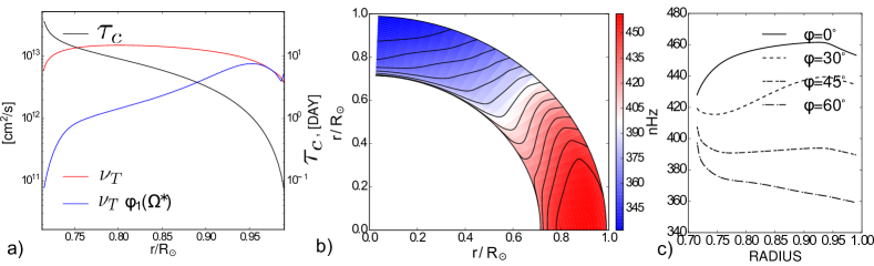
Figure 1: Convection zone properties from the MESA solar model: a) the convective turnover time, $\tau_{c}$ and the turbulent diffusivity parameter (red line), isotropic eddy viscosity is shown by blue line; b) the angular velocity profile of model M1 in the Northern hemisphere; c) the radial profile of the angular velocity for the different latitudes.

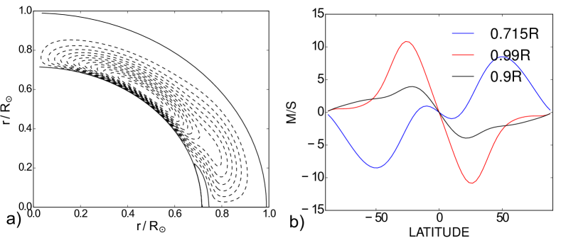
Figure 2: Model M1. a) Streamlines of the meridional flow ( stream function $\Psi$) shows a single-cell counterclockwise circulation pattern for the Northern hemisphere; b) velocity of the latitudinal component of the meridional flow for different radii.

In model M2 parameter $c_{\Lambda}$ is smaller than in model M1. The increase of the inward angular momentum flux due to the decrease of $c_{\Lambda}$ redistributes of the non-dissipative angular momentum fluxes. This results in an increase of the latitudinal shear. To compensate this effect we increase the Prandtl number from $1/3$ to $1/2$ (see, Table 1). The resulted pattern of the meridional flow has a triple-cell structure shown in Figure 3. This pattern consists of the two large counterclockwise circulation cells and a small clockwise cell located at low latitude at the bottom of the convection zone. The upper equatorial circulation cell has a stagnation point at the $r=0.86R$.

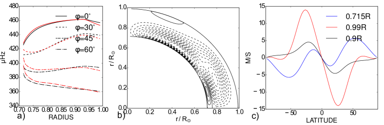
Figure 3: Model M2: a) the radial profiles of the angular velocity for different latitudes. The red color shows results for model M1 for comparison; b) the stream function distribution, the dashed lines show the counterclockwise circulation and the solid lines show the opposite circulation; c) velocity of the latitudinal component of the meridional flow for different radii.

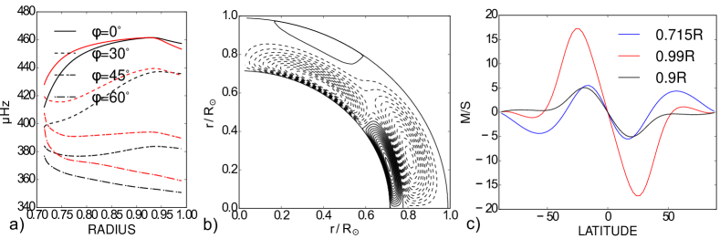
Figure 4: The same as in Figure 3 for the model M3.

Further increase of the inward angular momentum flux (via parameter $c_{\Lambda}$) results in amplification of the near equatorial clockwise circulation cell. This is illustrated by model M3 (Figure 4). This model has a slightly stronger latitudinal shear at the surface than model M1. The amplitude of the meridional flows in model M3 is larger than in M2. The flow speed reaches about 18 m/s at the surface and about 5 m/s at the bottom of the convection zone. Model M3 qualitatively preserves the angular velocity profile of model M1.

4 Discussion and conclusions

We investigated the mean-field models of the solar differential rotation using a simple description of the turbulent $\Lambda$-effect. Our goal was to study how the distributions of the non-dissipative angular momentum fluxes affects the meridional circulation structure in the solar convection zone. The study is motivated by the recent findings of helioseismology showing the existence of a double-cell meridional circulation pattern (Zhao et al., 2013), and also results of the global 3D numerical simulations which often demonstrate that circulation structure can be multicellular (see, e.g., Käpylä et al. (2011); Miesch et al. (2011); Guerrero et al. (2013).

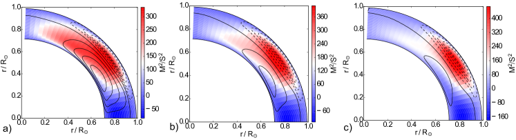
Figure 5: The Reynolds stresses $T_{r\phi}$ (background color) and $T_{\theta\phi}$ (contours, in the same range as $T_{r\phi}$), for models: a) M1; b) M2 ;c) M3.

Inspecting Eqs.(2.2,14) we see that the transport of angular momentum due to the turbulent $\Lambda$- effect changes from outward to inward near the equator. The near equatorial inward flux is minimal in model M1 and it grows with the decrease of parameter $c_{\Lambda}$. The non-monotonic spatial dependence of the angular momentum fluxes, and the extent of the near-equatorial region occupied by the inward non-dissipative angular momentum flux provides conditions for destabilization of the Taylor-Praudman balance, which results to the increasing complexity of the meridional circulation pattern.

Figure 5 illustrates the Reynolds stresses $T_{r\phi}$ and $T_{\theta\phi}$ for our set of models. In model M3, characterized by a triple-cell circulation pattern, the outward turbulent angular momentum fluxes are concentrated close to the surface in the mid-latitude of the solar convection zone. Also, in model M3 the amplitude of the inward flux near the equator is about factor three larger than in model M1. The turbulent Reynolds stress tensor component $T_{r\phi}$ is symmetric about the equator and $T_{\theta\phi}$ is anti-symmetric. Figure 5c (model M3) shows a similarity with the global 3D simulations results presented by Käpylä et al. (2011) (see Figures 4,5 for run A6 in their paper). Thus the origin of the multicellular merdional circulation pattern in their model can be explained by the latitudinal variations of the $\Lambda$-effect. This question should be studied further.

The rotation profiles in all three models are qualitatively similar, while model M1 is, probably, in the best agreement with the results of helioseismology inversions of Howe et al. (2011)m models M2 and M3 also have the radial profile of the angular velocity in qualitative agreement with helioseismology. Thus, we conclude that the multicellular meridional circulation structure can be explained by the mean-field models. However our models do not include the solar tachocline. From the results of Kitchatinov & Olemskoy (2011), we can guess that inclusion of the tachocline may affect the Taylor-Paudman balance near the bottom of the convection zone and change the magnitude of the meridonal circulation.

The turbulent part of the angular momentum transport is not well understood. The mean-field theory of the $\Lambda$-effect (Kichatinov & Rudiger, 1993) has some issues that are rarely discussed in the literature. The theory is constructed for forced isothermal turbulence rather than for turbulent convection. Calculation of Kleeorin & Rogachevskii (2006) show that the $\Lambda$-effect functions $V^{(0)}$ and $V^{(1)}$ may have dependence on the Coriolis number that is different from the results of Kichatinov & Rudiger (1993). Thus, theoretically, there is some uncertainty in the description of the turbulent angular momentum fluxes in rotating stellar convection zones. These uncertainties should be resolved using the global 3D numerical simulation and assimillation of the observational data in theoretical models.

Acknowledgments VP thanks support of RFBR under grant 15-02-01407 and the project II.16.3.1 of ISTP SB RAS.

Bibliography

Bibliography

- Guerrero et al. (2013) Guerrero, G., Smolarkiewicz, P. K., Kosovichev, A. G., & Mansour, N. N. 2013, ApJ, 779, 176
- Hathaway (2012) Hathaway, D. H. 2012, ApJ, 760, 84
- Howe et al. (2011) Howe, R., Larson, T. P., Schou, J., Hill, F., Komm, R., Christensen-Dalsgaard, J., & Thompson, M. J. 2011, Journal of Physics Conference Series, 271, 012061
- Käpylä et al. (2011) Käpylä, P. J., Mantere, M. J., Guerrero, G., Brandenburg, A., & Chatterjee, P. 2011, A & A, 531, A162
- Kholikov et al. (2014) Kholikov, S., Serebryanskiy, A., & Jackiewicz, J. 2014, ApJ, 784, 145
- Kichatinov et al. (1994) Kichatinov, L. L., Pipin, V., & Rüdiger, G. 1994, Astron. Nachr., 315, 157
- Kichatinov & Rudiger (1993) Kichatinov, L. L., & Rudiger, G. 1993, A & A, 276, 96
- Kitchatinov & Olemskoy (2011) Kitchatinov, L. L., & Olemskoy, S. V. 2011, MNRAS, 411, 1059
- Kitchatinov & Rüdiger (1999) Kitchatinov, L. L., & Rüdiger, G. 1999, A & A, 344, 911
- Kleeorin & Rogachevskii (2006) Kleeorin, N., & Rogachevskii, I. 2006, Phys. Rev. E, 73, 046303
- Küker & Rüdiger (2005) Küker, M., & Rüdiger, G. 2005, Astronomische Nachrichten, 326, 265
- Miesch et al. (2011) Miesch, M. S., Brown, B. P., Browning, M. K., Brun, A. S., & Toomre, J. 2011, in IAU Symposium, Vol. 271, IAU Symposium, ed. N. H. Brummell, A. S. Brun, M. S. Miesch, & Y. Ponty, 261–269
- Paxton et al. (2011) Paxton, B., Bildsten, L., Dotter, A., Herwig, F., Lesaffre, P., & Timmes, F. 2011, ApJ Supplement, 192, 3
- Paxton et al. (2013) Paxton, B., et al. 2013, ApJ Supplement, 208, 4
- Rempel (2005) Rempel, M. 2005, ApJ, 622, 1320
- Ruediger (1989) Ruediger, G. 1989, Differential rotation and stellar convection. Sun and the solar stars
- Zhao et al. (2013) Zhao, J., Bogart, R. S., Kosovichev, A. G., Duvall, Jr., T. L., & Hartlep, T. 2013, ApJL, 774, L29