Nonlinear waves on circle networks with excitable nodes

Abstract

Nonlinear wave formation and propagation on a complex network with excitable node dynamics is of fundamental interest in diverse fields in science and engineering. Here, we propose a new model of the Kuramoto type to study nonlinear wave generation and propagation on circular subgraphs of a complex network. On circle networks, in the continuum limit, this model is equivalent to the over-damped Frenkel-Kontorova model. The new model is shown to keep the essential features of those well-known models such as the diffusively coupled Bär-Eiswirth model but with much simplified expression such that analytic analysis becomes possible. We classify traveling wave solutions on circle networks and show the universality of its features with perturbation analysis and numerical computation.

I Introduction

Synchronization is a collective and emergent behavior of coupled agents which display spontaneous locking to a common oscillation frequency. The investigation of this ubiquitous and important phenomenon has been intense and fruitful in recent years. Much progress has been made in diverse fields, including examples from networks of pacemaker cells in the heart Peskin (1975); Michaels et al. (1987), metabolic synchrony in yeast cell suspensions Ghosh et al. (1971); Aldridge et al. (1976), congregations of synchronously flashing fireflies Buck (1988); Buck and Buck (1976), arrays of lasers Jiang and McCall (1993); Kourtchatov et al. (1995) or microwave oscillators York and Compton (1991) and wired superconducting Josephson junctions Wiesenfeld et al. (1996). It is probably one of the best examples of spontaneous emergence of rhythms in non-equilibrium systems. Different theoretical models have been proposed to study its onset and stability, among which the Kuramoto model is the most widely used for its simplicity in formulation and elegance in analysis. The majority of these models study coupled oscillators and check how the oscillation of individual members is shaped by different coupling strengths and topologies. Other dynamical aspects, such as the impact of noise, the finite-size effect and the co-evolution of structure and dynamics, have also been explored Acebrón et al. (2005); Hong et al. (2007). Different types of local dynamics are also explored to various extent with many interesting observations made Arenas et al. (2008) while much more remains to be probed Arenas et al. (2008).

The spatiotemporal pattern formation in excitable media has long been a hot topic for researchers in both applied and theoretical arena. If excitable dynamics is mounted on each node of a network, a discrete analogue of the excitable media is created, the collective dynamics of which critically depends on the network structure. Hu et. al recently investigated the diffusively coupled Bär-Eiswirth model and found that different nonlinear waves may emerge spontaneously with properly designed coupling strategy Qian et al. (2010). These nonlinear waves possess an interesting feature: the evolution on the neighboring nodes is equally separated in time but not in space. Based on the comprehensive numerical observation, they proposed an phase-advanced model which explains how all the nodes of the network are driven by a self-sustained central circle sub-network of oscillating nodes. Hence, dynamically a complex network can be viewed in a much simpler way: the central driving circle sub-network and the attached trees, which is determined by system dynamics. In Fig. 1, the nodes 1-6 make the circle subnetwork and 7-10 are attached as a tree branch. Once a driving circle network is selected dynamically, the oscillation on it will determine the behavior of the rest of the network. Therefore, it is crucial to identify possible spatiotemporal patterns on a circle network of excitable nodes with diffusive coupling.

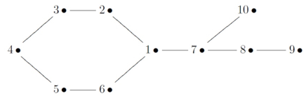
Figure 1: A simple example of a network with a circle sub-network.

In fact, the propagation of nonlinear waves along a circular track of excitable media was observed experimentally in heart muscles long ago and has been well explained based on empirical physiology models Frame and Simson (1988); Courtemanche et al. (1993). Similar waves were also observed in other low dimensional systems, such as the charge density waves in the quasi 1-d metals Grüner et al. (1989). In all these studies, a plethora of wave patterns were explored and their existence and stability were investigated with different analytical or numerical tools. However, in their mathematical description, the sophisticated set of coupled nonlinear differential equations often prevent an analytic approach and thus hinder our full understanding of the wave dynamics even in simple cases. Due to the universality of nonlinear wave propagation on networks, we feel that it is possible and necessary to find a model which keeps the essential features of those well-known models such as the diffusively coupled Bär-Eiswirth model but with much simplified description such that analytic analysis becomes possible.

Inspired by the success of the Kuramoto model in synchronization, we here propose a new model of similar type to target the problem of spatiotemporal pattern formation in a circle network with excitable node dynamics. We put a one-dimensional phase oscillator at each node, which is similar to the Kuramoto model but with nonuniform local frequency and diffusive coupling. The model is considerably simpler than the Bär-Eiswirth model used by Hu et. al Qian et al. (2010) but captures the essential dynamics. Specifically, detailed studies on spatiotemporal patterns in circle network have been carried out. Different spatiotemporal patterns in circle networks are observed, which can be compared and classified analytically according to the solution in the limit of uniform local frequency. Among all the nonlinear waves, the regular nonlinear wave, characteristic of its equal time-separation, is of great interest and significance. Further perturbation analysis indicates that the equal-time-separation solution is ubiquitous in the coupled excitable dynamics and it is stable. The restitution and dispersion curves of this wave bear remarkable similarity to those of a ring of excitable media, which implies universality of our model and its solutions. Other types of solutions, stable or unstable, are also found, including one special solution that seems to have no analogue in the continuum limit.

The equal-time-separation solution is related conceptually to the lag synchronization of two coupled nonidentical chaotic oscillators, in which physical observables of the two become synchronized but with a time lag Rosenblum et al. (1997). However, in our model, identical excitable phase oscillators are coupled diffusively and thus both the formed patterns and the underlying interaction between agents are different. In celestial mechanics, a remotely related example is the choreographic solution for the n-body problem, in which the moving bodies are also separated by a constant time interval Chenciner and Montgomery (2000). Henceforth, this equal-time-separation solution seems to be universal and much work is needed to reveal its manifestation and implication in different contexts.

This new model is an over-damped version of the well-known Frenkel-Kontorova model Braun and Kivshar (2004); Aubry and Le Daeron (1983); Bak (1982) which has become one of the fundamental and universal tools of low-dimensional nonlinear physics. The classical Frenkel-Kontorova model describes a chain of classical particles evolving on the real line, coupled with their neighbors and subjected to a periodic potential. In the continuum limit, i.e., the distance $a_{0}$ between neighboring nodes satisfies $a_{0}\ll 1$, the Frenkel-Kontorova model is reduced to the Sine-Gordon equation, which is a completely integrable nonlinear partial differential equation. The simplicity of the Frenkel-Kontorova model, as well as its surprising richness and capability to describe a range of important nonlinear phenomena has attracted a great deal of attention from physicists working in solid-state physics and nonlinear science, which provides a unique framework to combine many physical concepts and to make the analysis in a unified and consistent way. It is hopeful that our simplified version of the Frenkel-Kontorova model can also give interesting insights into the pattern formation in the context of complex networks.

The paper is organized as follows. In section II, we motivate the introduction of our model and a detailed discussion of its solution is made in section III. In particular, the stability condition and periods of regular solutions are analyzed with a perturbation approach. The regular nonlinear wave turns out to be a generic feature of circle networks with excitable node dynamics, which is discussed in detail in section III.2. The relation of the circulating pulse in the excitable media and the regular nonlinear wave is investigated in section IV with the dispersion and restitution curves being plotted. We summarize our results in section V.

II Our model

Much effort has been devoted to the study of nonlinear wave propagation or self-sustained oscillation on different types of networks. The Bär-Eiswirth model Bär and Eiswirth (1993) is recently used by Hu et. al,

$$\frac{du_{i}}{dt}=-\frac{1}{\epsilon}u_{i}(u_{i}-1)(u_{i}-\frac{v_{i}+b}{a})+\Delta^{2}u_{i}\,,$$ (1a)

$$\frac{dv_{i}}{dt}=f(u_{i})-v_{i}\,,$$ (1b)

where

$$f(u)=\begin{cases}0,&\quad u<\frac{1}{3}\\ 1-6.75u(u-1)^{2},&\quad\frac{1}{3}\leq u\leq 1\\ 1,&\quad u>1\,,\end{cases}$$

and $\Delta^{2}$ denotes the discrete Laplacian which can be defined on a bidirectional graph $D=<V,E>$ with the vertex set $V=\{v_{1},v_{2},...,v_{n}\}$ and the edge set $E=\{e_{1},e_{2},...,e_{m}\}$. With $a_{i,j}$ representing the number of edges from vertex $v_{i}$ to vertex $v_{j}$, the discrete Laplacian is

$$\Delta^{2}u_{i}=\sum_{j=1}^{n}a_{j,i}(u_{j}-u_{i}).$$ (2)

On a network of similar type as in Fig. 1, with Eq. (1), the dominant phase-advanced driving mechanism (DPAD) Qian et al. (2010) governs the dynamics. In Fig. 2(a) and 2(b), we show the dynamical behavior of all nodes if working with the network shown in Fig. 1. A circulating nonlinear wave is found on the circle sub-network with nearly uniform velocity, which indicates the equal time-separation between adjacent nodes. The small discrepancy is caused by the side branch attached. The dynamics of the nodes in the side branch is subordinate to that of node 1, as illustrated in Fig. 2(b). The DPAD mechanism, i.e., a cascading driving ladder relaying sustained oscillations, is vividly shown in Fig. 2(b). For example, node 7 is always pulled by node 1 away from the stable fixed point of the local dynamics. The circle sub-network plays an essential role in the current network which motivates an in-depth investigation on the possible dynamical behavior of a circle network with various local dynamics to find out universality of the wave propagation. Below, we will take one of the simplest case, i.e., a particular one-dimensional equation as the local dynamics.

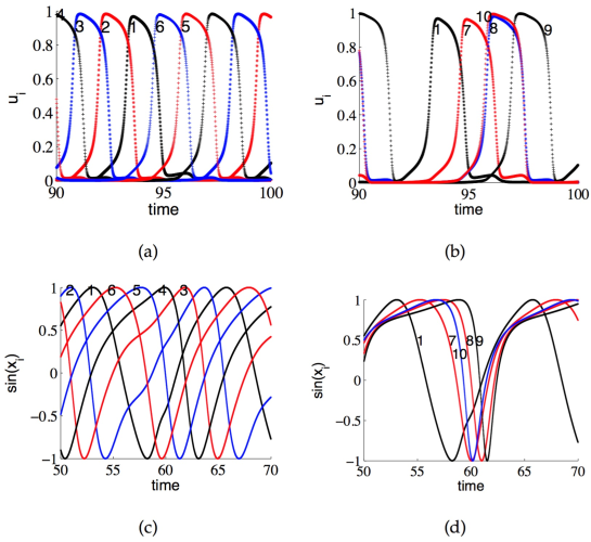
Figure 2: Nonlinear waves on the network displayed in Fig. 1. (a), (b) Dynamics (i.e., $u_{i}(t)$, plotted as ‘*’ or ‘+’) of different nodes for Eq. (1) with $\epsilon=0.04,\,b=0.07,\,a=0.84,\,d=0.2$: for nodes (a) in the circle sub-network and (b) in the attached tree branch. (c), (d) Corresponding dynamics for Eq. (4) with $w=0.8,\,\epsilon=1,\,d=1$, for nodes (c) in the circle sub-network and (d) in the branch. Note that the vertical coordinate for (c) and (d) is $\sin(x_{i})$ so that the similarity between (a) (b) and (c) (d) is more apparent.

A general equation of motion with local 1-d dynamics and nearest neighbor interaction along a circle network could be written as:

$$\dot{x_{i}}=f(x_{i})+R(x_{i-1},x_{i},x_{i+1}),\,\,\,\,i\in\{1,2,3,....,n\}\,\,,\;x_{i}\in\mathbb{R}$$ (3)

where $f(x_{i})$ denotes the local dynamics and $R(x_{i-1},x_{i},x_{i+1})$ is the coupling term between neighboring nodes. The total number of nodes is assumed to be $n$ and due to circle topology, $x_{i\pm n}=x_{i}$. The dynamics is invariant under the rotation $x_{i}\rightarrow x_{i+k},\forall k\in\mathbb{N}$, the reflection $x_{i}\rightarrow x_{n+1-i}$ and their group composite. The periodicity also implies a simple composition rule. Suppose the variables $\{x_{i}(t)\}_{i=1,2,...,p}$ and $\{y_{i}(t)\}_{i=1,2,...,mp}$ describe dynamics governed by the same equation of motion (3) on two circle networks with $p$ and $mp$ nodes respectively. The identification $y_{i}=x_{j}\,,\mbox{ for }i=j(\mathrm{mod}\,p)\,,i=1,2,...,mp$ will generate a solution for the $y$-system for any $x$-solution, as illustrated in Fig. 4. Dynamics in Fig. 4(d) is inherently a spatial juxtaposition of that in Fig. 4(g).

For simplicity, without loss of generality, we will mainly use the diffusion model below

$$\dot{x}_{i}=\omega-\epsilon\sin(x_{i})+d\sin(\Delta^{2}x_{i}),\,\,\,\,i\in\{1,2,3,....n\},\;x_{i}\in\mathbb{R}$$ (4)

where $\Delta^{2}$ is the Laplacian operator, as defined in Eq. (2). For circle networks, $\Delta^{2}x_{i}=x_{i+1}+x_{i-1}-2x_{i}$. The local dynamics is identical to that of the Kuramoto model if $\epsilon=0$. Besides, the case $\epsilon>\omega$ corresponds to the so-called theta-neuron model, also known as Ermentrout-Kopell model Ermentrout and Kopell (1986) and the case $\epsilon<\omega$ is widely investigated in the field of Josephson junctions Wiesenfeld et al. (1998). When $\epsilon$ is greater than but close to $\omega$, a stable and an unstable equilibria exist on the phase circle of the local dynamics, and the system becomes excitable: all the orbits go to the unique stable equilibrium unless a perturbation brings the state over the unstable one which induces a large excursion. Compared to the usual 2-dimensional excitable dynamics equation Eq. (1), the current one is much simpler so that a relatively thorough discussion of its solution becomes possible. In the continuum limit, the wavelength $\lambda\gg 1$ and $\Delta x_{i}=x_{i+1}+x_{i-1}-2x_{i}\ll 1$, so that $\sin(\Delta^{2}x_{i})\rightarrow\Delta^{2}x_{i}$. The wavelength $\lambda$ is measured in terms of the number of nodes that are spanned with a period of the wave oscillation. The term $\sin(\Delta^{2}x_{i})$ is invariant under a phase shift of $x_{i}\to x_{i}+2k_{i}\pi,k_{i}\in\mathbb{Z}$, which is convenient to analyze in the current context.

With Eq. (4), the dynamical behavior of all nodes in Fig. 1 is displayed in Fig. 2(c) and (d). The dynamical behavior in Fig. 2(c) looks similar to that in Fig. 2(a). Hence, the simple one-dimensional Eq. (4) seems to have captured the essential features of the Bär-Eiswirth model (1), though the precise wave profiles are not identical. Here, we emphasize that although the interaction between the circle sub-network and the branch network is mutual, the DPAD mechanism governs the uni-directional propagation of action, as clearly seen in Fig. 2(d). The back reaction of the branch on the circle network is small, so the equal-time-separation profile is well preserved. For a general nonlinear wave propagation, this may not be the case. The observed DPAD structure is intimately related to the excitable node dynamics. Our model Eq. (4) well captures this particular feature of the dynamics.

Our new model is closely related to the Frenkel-Kontorova model which describes harmonically coupled particle chain moving in a periodic potential. If $\phi$ denotes the position of the particle $i\in\mathbb{Z}$, one of the simplest Frenkel-Kontorova models could be written as

$$m\frac{d^{2}\phi}{dt^{2}}+\gamma\frac{d\phi_{i}}{dt}=L+\sin(\phi_{i})+\Delta^{2}\phi_{i},$$

where $m$ is the particle mass, $\gamma$ a friction coefficient and $L$ is a constant driving force. The term $\sin(\phi_{i})$ is the force exerted by a periodic potential and the interaction $\Delta^{2}\phi_{i}=\phi_{i+1}+\phi_{i-1}-2\phi_{i}$ is diffusive.

In the over-damped limit $m\ll\gamma=1$, we neglect the inertial term and obtain

$$\frac{d\phi_{i}}{dt}=L+\sin(\phi_{i})+\Delta^{2}\phi_{i}.$$ (5)

As an application, this simplified model reproduces the complex behavior of the charged density waves (CDWs), including the depinning transition, mode-locking, and sub-threshold hysteresis Middleton (1992); Pietronero and Strässler (1983); Matsukawa and Takayama (1984), where $\phi_{i}$’s describe the configuration of the charged density wave. Our model when implemented on circle networks is equivalent to the over-damped Frenkel-Kontorova model in the continuum limit since $\sin(\Delta^{2}x_{i})\to\Delta^{2}x_{i}$ in that limit.

Strogatz et. al also used the model below to characterize the CDW on a ring Strogatz et al. (1988),

$$\dot{\phi_{i}}=L-h\sin(\phi_{i}-\alpha_{i})+\frac{K}{n}\sum_{j=1}^{n}\sin(\phi_{j}-\phi_{i})\,.$$ (6)

The main difference between Eq. (6) and our model Eq. (4) is that the coupling term in Eq. (6) is global rather than local as in our model.

To visualize the dynamical behavior of Eq. (4), it is convenient to denote the state of a node by a point on a circle (phase space of the local dynamics) and so the state of the whole system can be represented by a group of points on the same circle. If $d=0$ in Eq. (4), then each point will move along the circle according to the local dynamics while for $d\neq 0$ the points will interact with their nearest neighbors. When $\lvert w\rvert<\lvert\epsilon\rvert$, the local dynamics indicate a unique stable fixed point while the interaction may push nodes away from this stable equilibrium. In fact, a threshold coupling exists which delimits regimes for stable fixed configuration and for stable circulation along the circle, i.e., a stable nonlinear wave on the network. The simplicity of the model enables a detailed analysis of this oscillatory solutions as shown in next section.

III Spatiotemporal patterns

Let’s consider the equation below

$$\dot{x_{i}}=w+d\sin(x_{i+1}+x_{i-1}-2x_{i})\,,x_{i}\in\mathbb{R}$$ (7)

which is the special case $\epsilon=0$ of Eq. (4). In this simplified equation, a two-parameter continuous symmetry group comes to existence: the equation is invariant under $x_{m}\to x_{m}+c_{1}+mc_{2}\,,\forall c_{1}\,,c_{2}\in\mathbb{R}$. Of course, the boundary conditions should be satisfied under this transformation. For the periodic boundary condition, $c_{2}$ can only take discrete values. With the notation

$$\eta_{i}=\begin{cases}x_{i+1}-x_{i},\quad&i\in\{1,2,...,n-1\}\\ x_{1}-x_{n},\quad&i=n\,,\\ \end{cases}$$

Eq. (7) becomes

$$\frac{d\eta_{i}}{dt}=d\sin(\eta_{i+1}-\eta_{i})-d\sin(\eta_{i}-\eta_{i-1})\,,$$ (8)

with the constraints $\sum_{i}^{n}\eta_{i}=2k\pi\,,\eta_{n+1}=\eta_{1}+2p\pi\,,\;k,p\in\mathbb{Z}$ due to periodicity.

III.1 General solutions

Any stationary solution for Eq. (8) satisfies

$$\,\,\eta_{i+1}-\eta_{i}=\beta\mbox{ or }\pi-\beta\,,\,\forall i\,,$$ (9)

where $\beta$ is a constant chosen to satisfy the periodic boundary condition. So, the structure of the general solution is rather complex even for the simplified equation. If there exist $j$’s such that both choices of Eq. (9) are made, in the continuum limit, $\beta\to 0\,,\pi-\beta\to\pi$, the resulting solution does not correspond to physical reality, which hence only appears when the interacting units are discrete. Below is a simple case with alternating choice of the two values

$$\eta_{2i}-\eta_{2i-1}=\beta\,,\eta_{2i+1}-\eta_{2i}=\pi-\beta\,,\,\,i\in 1,2,..,\mbox{ for }n=4m\,,m\in\mathbb{N}\,.$$

We then have

$$\eta_{2}=\eta_{1}+\beta,\,\eta_{3}=\eta_{1}+\pi,\,\eta_{4}=\eta_{1}+\pi+\beta,\mbox{ and }\eta_{i+4}=\eta_{i}+2\pi\,,$$

where $\beta=k\pi/m$ to satisfy the periodicity condition when we take $\eta_{1}=0$ for simplicity. Therefore,

$$x_{2}=x_{1},\,x_{3}=x_{1}+\beta,\,x_{4}=x_{1}+\pi+\beta\mbox{ and }x_{i}=x_{i-4}+2\pi+2\beta\,,\mbox{ for }i>4\,,$$ (10)

which is a rather complex wave on the circle network. Possible unstable nonlinear waves of this type are abundant, as illustrated in Fig. 3. For all solutions in Fig. 3, they are checked numerically to be unstable. However, a proof for the stability of a general solution does not seem to be easy.

In order to describe waves on a circle network, a triple-plot set is used throughout this paper, among which the first plot depicts the time course for each node, the second plot takes a snapshot of this dynamic wave and marks the profile in the phase space, and the third one displays the state of each node in the second plot. This protocol is demonstrated in Fig. 3.

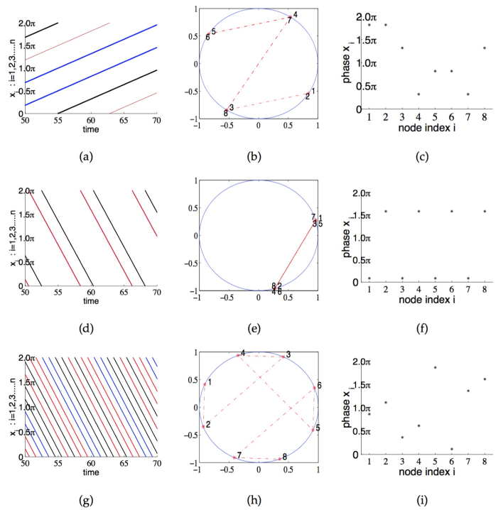
Figure 3: Some interesting unstable waves on the circle network with $n=8$. (a) An unstable wave on the circle network, corresponding to Eq. (10) with $w=0.8,\,\epsilon=0,\,d=1$. (b) The phase space configuration of a snapshot of the unstable wave in (a). (c) The corresponding $x_{i}$ value on each node in (b). The plots (d), (e), (f) and (g), (h), (i) correspond to two other unstable waves on the same circle network.

A more interesting case satisfies $\eta_{i+1}-\eta_{i}=\beta$ invariably such that

$$\eta_{i}=\eta_{1}+(i-1)\beta\,.$$ (11)

But with the periodicity condition following Eq. (8), we have the constraint

$$\beta=\frac{2p\pi}{n}\,,\;\eta_{1}=\frac{2k\pi-(n-1)p\pi}{n}\,.$$ (12)

The solution for the phase variable $x_{i}$ is

$$x_{i}=(\omega+d\sin\beta)t+(i-1)\eta_{1}+\frac{(i-1)(i-2)}{2}\beta+x_{00}\,,$$ (13)

where $x_{00}$ is some arbitrary initial phase. The stability of this solution is discussed in Appendix A. In section III.3, we will discuss several special cases for this general solution when $\beta\neq 0$, which are stable for $d\cos\beta>0$ according to Appendix A and referred to as special solutions or special waves in the current paper.

When going to the continuum limit, only the solutions with $\beta=0\,(p=0)$ makes physical sense so that the phase separations become equal, which is referred to as the regular solution or regular wave and will be further investigated in detail later. Under this condition Eq. (13) is much simplified:

$$x_{i}=\omega t+\frac{2(i-1)k\pi}{n}+x_{00}\,.$$ (14)

Note that the natural frequency is restored. According to Appendix A, regular waves are stable. As we will see, the regular wave will persist even for $\epsilon\neq 0$, where the phase-space separations between $x_{i}$’s would be non-constant but their temporal separations remain constant.

In this section, possible solutions of the model Eq. (4) are classified or discussed briefly. Among stable solutions, we identified the regular and the special waves. Furthermore, through extensive numerical experiments we found that in the region where nontrivial asymptotic solutions exist, basin of attraction for regular waves or static solutions covers a large portion of the phase space. In another word, these types of solutions most likely appear when starting from an initial condition chosen randomly, which greatly facilitates exploration of the phase space orbit structure.

III.2 The universality of regular nonlinear waves

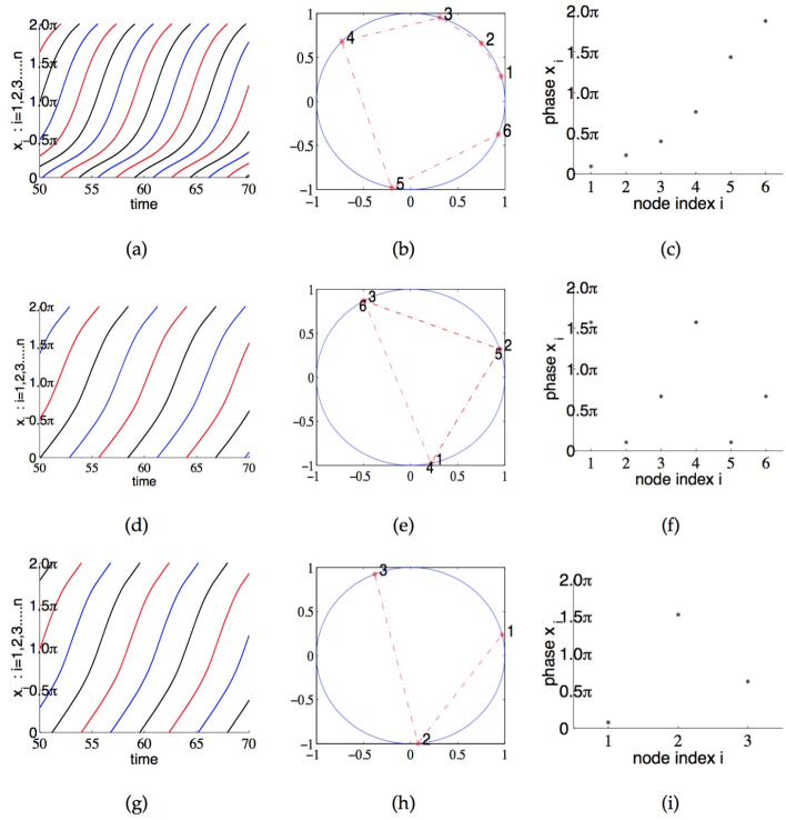
Figure 4: Regular nonlinear waves on the circle network with $w=0.8,\,\,\epsilon=1,\,\,d=1$. See Eq. (26). $\langle$(a), (b), (c)$\rangle$ A regular nonlinear wave with $k=1,\,n=6$. $\langle$(d), (e), (f)$\rangle$ A regular nonlinear wave with $k=2,\,n=6$. $\langle$(g), (h), (i)$\rangle$ A regular nonlinear wave with $k=1,\,n=3$.

The regular wave survives perturbation and continues to exist even when $\epsilon$ grows as large as $\omega$ or $d$, as shown in Fig. 4. In circle networks, regular nonlinear waves are the most commonly observed ones, which are attributed to the rotational symmetry of the system and quite independent of the local dynamics. We will make a perturbation analysis to a generalized equation to derive the expression of the period and the analytical form of the regular solution to the lowest order, thus showing the universal features of regular nonlinear waves.

Let’s consider a generalized form of Eq. (4)

$$\dot{x_{i}}=\omega-\epsilon g(x_{i})+h(x_{i+1}+x_{i-1}-2x_{i}),\;x_{i}\in\mathbb{R}\,,$$ (15)

where $g\,,h$ are both smooth $2\pi$-periodic functions with $h(0)=0,h^{\prime}{}(0)>0,\,h^{\prime}{}^{\prime}{}(0)=0,\,\text{and}\,\int_{0}^{2\pi}g(x)dx=0$. Note that if $h(0)\neq 0$, then $h(0)$ can be incorporated into $\omega$. Besides, it is assumed that $a_{0}=\int_{0}^{2\pi}g(x)dx=0$, otherwise, the transformation

$$g(x)\rightarrow g(x)-a_{0},\,\,\,\omega\rightarrow\omega-\epsilon a_{0}$$

gives the right form.

The Poincaré-Lindstedt method Verhulst (1996) is a well-known perturbation approach for approximating periodic solutions of ordinary differential equations. An introduction to the technique and the justification of its usage here are given in Appendix B. Below, by applying the Poincaré-Lindstedt perturbation technique, we compute the period and the analytic form of the regular nonlinear wave to the lowest order of $\epsilon$. Its stability is also discussed. For $\epsilon\ll 1$, we assume that the time and the state variable have the following form

$$\tau = \Omega t\,,$$

$$\Omega = \omega_{0}+\epsilon\omega_{1}+\epsilon^{2}\omega_{2}+...\,,$$

$$x_{i} = x_{i,0}+\epsilon x_{i,1}+\epsilon^{2}x_{i,2}+...\,.$$ (16)

Then $x_{i}(\tau)$ is $2\pi$-periodic and the period for $x_{i}(t)$ is $2\pi/\Omega$. After substitution of Eq. (16) into Eq. (15), a comparison of different orders of $\epsilon$ leads to

$$1:\,\,\,\omega_{0}\frac{dx_{i,0}}{d\tau}=\omega+h(x_{i+1,0}+x_{i-1,0}-2x_{i,0})\,,$$ (17)

$$\epsilon:\,\,\omega_{1}\frac{dx_{i,0}}{d\tau}+\omega_{0}\frac{dx_{i,1}}{d\tau}=g(x_{i,0})+h^{\prime}{}(x_{i+1,0}+x_{i-1,0}-2x_{i,0})(x_{i+1,1}+x_{i-1,1}-2x_{i,1})\,,$$ (18)

$$\begin{split}\epsilon^{2}:\,\,\omega_{0}\frac{dx_{i,2}}{d\tau}+\omega_{1}\frac{dx_{i,1}}{d\tau}+\omega_{2}\frac{dx_{i,0}}{d\tau}&=x_{i,1}g^{\prime}{}(x_{i,0})+(x_{i+1,2}+x_{i-1,2}-2x_{i,2})h^{\prime}{}^{\prime}{}(x_{i+1,0}+x_{i-1,0}-2x_{i,0})\\ &+\frac{1}{2}h^{\prime}{}^{\prime}{}(x_{i+1,0}+x_{i-1,0}-2x_{i,0})(x_{i+1,1}+x_{i-1,1}-2x_{i,1})^{2}\,.\end{split}$$ (19)

With the definition $\eta_{i}=x_{i+1,0}-x_{i,0}$, Eq. (17) becomes

$$\omega_{0}\frac{d\eta_{i}}{d\tau}=h(\eta_{i+1}-\eta_{i})-h(\eta_{i}-\eta_{i-1})\,.$$

The regular nonlinear wave takes the form $\eta_{i}=-2k\pi/n,\,k=0,1,2,3,...n-1$. Then $\omega_{0}=\omega$ and

$$x_{i,0}=\tau-\frac{2(i-1)k\pi}{n}\,,$$

which is a stable regular solution of Eq. (17). Eq. (18) then becomes

$$\omega_{1}+\omega\frac{dx_{i,1}}{d\tau}=g\Big{(}\tau-\frac{2(i-1)k\pi}{n}\Big{)}+h^{\prime}{}(0)(x_{i+1,1}+x_{i-1,1}-2x_{i,1})\,,$$

which, upon substitution of the Fourier expansion for $g(\tau-\frac{2(i-1)k\pi}{n})$, gives

$$\begin{split}\omega_{1}+\omega\frac{dx_{i,1}}{d\tau}&=\sum_{m=1}^{\infty}\Big{(}a_{m}\sin\big{(}m(\tau-\frac{2(i-1)k\pi}{n})\big{)}+b_{m}\cos(m(\tau-\frac{2(i-1)k\pi}{n}))\Big{)}\\ &+h^{\prime}{}(0)(x_{i+1,1}+x_{i-1,1}-2x_{i,1})\,,\end{split}$$ (20)

where $a_{m}\,,b_{m}$ are the Fourier coefficients for $g(x)$. Let $v_{0}=\sum_{i=1}^{n}x_{i,1}$ and a summation of the above equation over $i$ gives

$$\begin{split}n\omega_{1}+\omega\frac{dv_{0}}{d\tau}&=\sum_{m=1}^{\infty}\left\{a_{m}\sum_{i=1}^{n}\Big{(}\sin\big{(}m(\tau-\frac{2(i-1)k\pi}{n})\big{)}\Big{)}+b_{m}\sum_{i=1}^{n}\Big{(}\cos\big{(}m(\tau-\frac{2(i-1)k\pi}{n})\big{)}\Big{)}\right\}\\ &\,\,\,\,+h^{\prime}{}(0)\sum_{i=1}^{n}(x_{i+1,1}+x_{i-1,1}-2x_{i,1})\\ &=0+0+0\\ &=0\,.\end{split}$$

To avoid secular terms in $v_{0}$, $\omega_{1}=0$ is taken, thus obtaining the periodicity condition

$$\begin{split}\omega\frac{dx_{i,1}}{d\tau}&=\sum_{m=1}^{\infty}\Big{(}a_{m}\sin(m(\tau-\frac{2(i-1)k\pi}{n}))+b_{m}\cos(m(\tau-\frac{2(i-1)k\pi}{n}))\Big{)}\\ &+h^{\prime}{}(0)(x_{i+1,1}+x_{i-1,1}-2x_{i,1})\,.\end{split}$$ (21)

Note that Eq. (21) is a linear differential equation with the driving term being a superposition of trigonometric functions. Hence, the response is a superposition of solutions for the component-wise equation,

$$\dot{f}_{i}=\frac{a_{m}}{\omega}\sin(m(\tau-\frac{(i-1)2k\pi}{n}))+\frac{h^{\prime}{}(0)}{\omega}(f_{i+1}+f_{i-1}-2f_{i})\,,$$

$$\dot{q}_{i}=\frac{b_{m}}{\omega}\cos(m(\tau-\frac{(i-1)2k\pi}{n}))+\frac{h^{\prime}{}(0)}{\omega}(q_{i+1}+q_{i-1}-2q_{i})\,.$$

According to Eq. (45) and Eq. (46) in Appendix C, the solution is

$$f_{i}=a_{m}A_{m}\sin(m(\tau-\frac{(i-1)2k\pi}{n}))+a_{m}B_{m}\cos(m(\tau-\frac{(i-1)2k\pi}{n}))\,,$$

$$q_{i}=-b_{m}B_{m}\sin(m(\tau-\frac{(i-1)2k\pi}{n}))+b_{m}A_{m}\cos(m(\tau-\frac{(i-1)2k\pi}{n}))\,.$$

where

$$A_{m}=\frac{4h^{\prime}{}(0)\sin^{2}(k\pi/n)}{m^{2}\omega^{2}+(4^{\prime}{h}(0)\sin^{2}(mk\pi/n))^{2}},B_{m}=-\frac{m\omega}{m^{2}\omega^{2}+(4^{\prime}{h}(0)\sin^{2}(mk\pi/n))^{2}}\,.$$

Then

$$x_{i,1}=\sum_{m=1}^{\infty}\Big{(}(a_{m}A_{m}-b_{m}B_{m})\sin(m(\tau-\frac{(i-1)2k\pi}{n}))+(a_{m}B_{m}+b_{m}A_{m})\cos(m(\tau-\frac{(i-1)2k\pi}{n}))\Big{)}\,.$$

Eq. (19) with substitution of $x_{i,0},\,\,x_{i,1}$ and the assumption that $h^{\prime}{}^{\prime}{}(0)=0$ (so complicated nonlinear terms disappear) gives

$$\omega_{2}+\omega\frac{dx_{i,2}}{d\tau}=h^{\prime}{}(0)(x_{i+1,2}+x_{i-1,2}-2x_{i,2})\\ +\sum_{m=1}^{\infty}\Big{(}a_{m}m\cos(m(\tau-\frac{2(i-1)k\pi}{n}))-b_{m}m\sin(m(\tau-\frac{2(i-1)k\pi}{n}))\Big{)}\\ \times\sum_{m=1}^{\infty}\Big{(}(a_{m}A_{m}-b_{m}B_{m})\sin(m(\tau-\frac{(i-1)2k\pi}{n}))+(a_{m}B_{m}+b_{m}A_{m})\cos(m(\tau-\frac{(i-1)2k\pi}{n}))\Big{)}\,.$$ (22)

Let $v_{1}=\sum_{i=1}^{n}x_{i,2}$, sum over $i$ and integrate from 0 to $2\pi$ the above equation:

$$\begin{split}2\pi n\omega_{2}+\int_{0}^{2\pi}\omega\frac{dv_{1}}{d\tau}&=\sum_{m=1}^{\infty}\sum_{i=1}^{n}\Big{\{}\int_{0}^{2\pi}\Big{(}-b_{m}m(a_{m}A_{m}-b_{m}B_{m})\sin^{2}(m(\tau-\frac{2(i-1)k\pi}{n}))\Big{)}d\tau\\ &+\int_{0}^{2\pi}a_{m}m(a_{m}B_{m}+b_{m}A_{m})\cos^{2}(m(\tau-\frac{2(i-1)k\pi}{n}))d\tau\Big{\}}\\ &=\sum_{m=1}^{\infty}\Big{(}mn\pi(a_{m}^{2}B_{m}+b_{m}^{2}B_{m})\Big{)}\,.\end{split}$$

To avoid secular terms in $v_{1}$, we take

$$\omega_{2}=\frac{\sum_{m=1}^{\infty}m(a_{m}^{2}B_{m}+b_{m}^{2}B_{m})}{2}\,.$$

In the end, we obtain a solution, which is stable J.K.Hale (1963),

$$x_{i}=\tau-\frac{2(i-1)k\pi}{n}+\epsilon\sum_{m=1}^{\infty}\Big{(}(a_{m}A_{m}-b_{m}B_{m})\sin(m(\tau-\frac{(i-1)2k\pi}{n}))\\ +(a_{m}B_{m}+b_{m}A_{m})\cos(m(\tau-\frac{(i-1)2k\pi}{n}))\Big{)}+O(\epsilon^{2})\,,$$ (23)

with

$$\Omega=\omega+\frac{\sum_{m=1}^{\infty}m(a_{m}^{2}B_{m}+b_{m}^{2}B_{m})}{2}\epsilon^{2}+O(\epsilon^{3})\,,$$ (24)

$$T=\frac{2\pi}{\omega}-\frac{\sum_{m=1}^{\infty}m\pi(a_{m}^{2}B_{m}+b_{m}^{2}B_{m})}{\omega^{2}}\epsilon^{2}+O(\epsilon^{3})\,,$$ (25)

where $\tau=\Omega t$ and

$$A_{m}=\frac{4h^{\prime}{}(0)\sin^{2}(mk\pi/n)}{(m\omega)^{2}+(4h^{\prime}{}(0)\sin^{2}(mk\pi/n))^{2}},\,\,\,\, a_{m}=\frac{1}{\pi}\int_{0}^{2\pi}\sin(x)g(x)dx\,,$$

$$B_{m}=-\frac{m\omega}{(m\omega)^{2}+(4h^{\prime}{}(0)\sin^{2}(mk\pi/n))^{2}},\,\,\, b_{m}=\frac{1}{\pi}\int_{0}^{2\pi}\cos(x)g(x)dx\,.$$

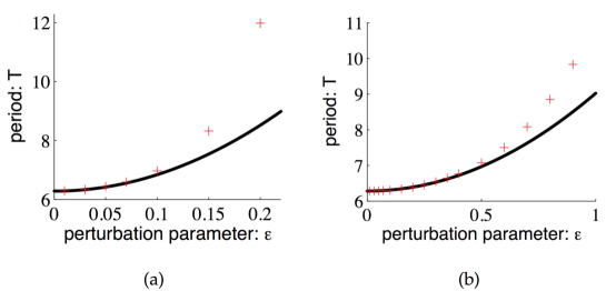
Figure 5: The dependence of $T(\epsilon)$ on $\epsilon$ of regular nonlinear waves. Simulation results are plotted as plus($+$), while the analytical prediction is plotted as a solid line. (a) Results from the system described by $\dot{x_{i}}=1-\epsilon(\sin(x_{i})+2\cos(2x_{i})+3\sin(3x_{i})+4\cos(4x_{i}))+\sin(x_{i+1}+x_{i-1}-2x_{i}),$ with $n=10,k=1$. The analytical prediction is $T=54.9444\epsilon^{2}+6.2832$ according to Eq. (25). (b) Results from the system described by Eq. (4) with $n=10,\,\,w=1,\,\,d=1,\,\,k=1$. The analytical prediction is $T=2.7415\epsilon^{2}+6.2831+O(\epsilon^{3})$, based on Eq. (27).

The above perturbation analysis validated our vision that, in the context of circle networks, regular nonlinear waves exist stably as long as Eq. (15) is satisfied. Regular nonlinear waves for different local dynamics on circle networks have been simulated and invariably observed. In Fig. 5(a), we gave an example where the period $T(\epsilon)$ vs $\epsilon$ is plotted. When $\epsilon<0.1$, the analytical results fit quite well with the simulation results. However, when $\epsilon>0.1$ the analytical results start to diverge, higher order terms coming into play.

Based on the above analysis and the resulting Eq. (23), (24) and (25), we have the following perturbation solution for Eq. (4) which is a special case of Eq. (15)

$$x_{i}=\tau-\frac{(i-1)2k\pi}{n}+\epsilon\left(B\cos\Big{(}\tau-\frac{(i-1)2k\pi}{n}\Big{)}+A\sin\Big{(}\tau-\frac{(i-1)2k\pi}{n}\Big{)}\right)+O(\epsilon^{2})\,,$$ (26)

$$\Omega=\omega-\frac{B}{2}\epsilon^{2}+O(\epsilon^{3})\,,$$

$$T=\frac{2\pi}{w}+\frac{B\pi}{w^{2}}\epsilon^{2}+O(\epsilon^{3})\,,$$ (27)

where

$$\tau=\Omega t,\,\,A=-\frac{4d\sin^{2}(k\pi/n)}{w^{2}+16d^{2}\sin^{4}(k\pi/n)},\,\,B=\frac{w}{w^{2}+16d^{2}\sin^{4}(k\pi/n)}\,.$$

In Fig. 4(a) and (d), it is easy to see that the nonlinear wave has the property of equal time separation, while the phase space separations between $x_{i}$’s are different, as illustrated in Fig. 4(c) and (f). In the case of Eq. (26), the phase separation $\Delta t=kT/n$ for $k\neq 0$. When $k=0$, all the nodes fully synchronize and there is no phase difference.

Thus, the perturbation analysis gives the nonlinear wave solution and it is stable when $d>0$. On the circle network, the variable $k$ in Eq. (26) indicates the wavenumber for the nonlinear wave. The corresponding wavelength $\lambda$ is $n/k$. Regular nonlinear waves with different wavenumbers are shown in Fig. 4. In the phase space, wavenumbers can be easily calculated by counting the number of circuits for which the consecutive node $1,2,..,n$ winds around the circle. Thus, the wavenumber is $1$ for Fig. 4(b) and $2$ for Fig. 4(e). From Eq. (27), it is easy to see that both the period and the frequency depend on $\epsilon$ quadratically to the lowest order. The configuration is recurrent on the circle network in a regular time interval $T$. The dependence of $T$ on $\epsilon$ is computed numerically and agrees quite well with the analytical approximation Eq. (27) for $\epsilon<0.5$, as shown in Fig. 5(b). For bigger $\epsilon$, the actual period is larger than the analytical result, which indicates a non-negligible role of higher order terms. It is expected that at some finite value of $\epsilon$ depending on the coupling $d$ and the wavenumber $k$, the regular nonlinear wave ceases to exist and the stable solution is a fixed point which corresponds to a uniform and stationary phase configuration.

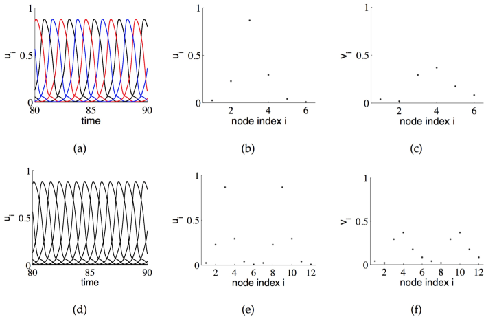
Figure 6: Regular nonlinear waves on the circle network for the revised Bär-Eiswirth model, with $\epsilon=0.04,\,\,b=0.15,\,\,a=0.84,\,\,d=1$, see Eq. (1). In (a), (b), (c), a regular nonlinear wave with $k=1,\,n=6$, where (a) depicts the dynamics of $u_{i}(t)$, (b) shows a snapshot of $u_{i}$ and (c) shows a snapshot of $v_{i}$. In (d), (e), (f), a regular nonlinear wave with $k=2,\,n=12$.

The regular nonlinear waves in the current model are closely related to those of the two-dimensional models, such as the Bär-Eiswirth model (1). Regular nonlinear waves with wavenumbers $k=1,\,\,2$ for the Bär-Eiswirth model are depicted in Fig. 6. In Fig. 6(d), the node $i$ and node $(i+6)(mod\,12)$ synchronize, resulting from the periodicity of the circle network. The nonlinear wave in Fig. 6(d) is actually constructed from the one in Fig. 6(a). In simulation, regular nonlinear waves for $n<6$ have not been found. By comparing Fig. 4 and Fig. 6, we see that regular nonlinear waves are simple yet universal for circle networks, which are significant to the analysis of pattern formation in complex networks.

A key concept from the Frenkel-Kontorova model is the phase gradient across the system, i.e., $\Delta x_{i}=x_{i}-x_{i-1}$. The analysis in this work mainly addresses the case of a constant phase gradient, i.e., regular solutions for $\epsilon\to 0$. Given an arbitrary initial condition, regular nonlinear waves are more likely to be selected according to our simulation. This can be partly explained in terms of the soliton which is a fundamental solution for the Frenkel-Kontorova model. More complicated wave patterns can be constructed with multiple solitons. Presumably, due to the repulsive interaction between the solitons, the phase gradient tends to become uniform when the lattice pinning effect Braun and Kivshar (2004) vanishes, i.e., $\epsilon\to 0$, thus resulting in regular nonlinear waves.

III.3 Stable solutions with $\beta\neq 0$

Stable solutions for $\beta\neq 0$ are also observed and only appear in the discrete case, as illustrated in Fig. 7. This special type of solutions, if viewed as nonlinear waves, has nearly all nodes synchronized in pairs, leaving one (when $n$ is odd) or two (when $n$ is even) nodes moving alone.

In the general solution (13), when n is odd, we may take $k=(n+1)/2$ in the constraint Eq. (12) such that $\eta_{1}=\beta$. In this case,

$$x_{i}=x_{n+1-i},i\in\{1,2,3,..,\frac{n-1}{2}\}\,.\\$$ (28)

When $n$ is even, we may take $k=n/2$ in Eq. (12) so that $\eta_{1}=\beta/2$. In this case,

$$x_{i}=x_{n+2-i},i\in\{2,3,..,\frac{n}{2}\}\,.$$ (29)

The discussion above is also applicable to the circumstance with $\epsilon>0$. Fig. 7 demonstrates two special typical nonlinear waves with $\epsilon=0.05$. In Fig. 7(b), we see that the node pairs $(1,7),\,(2,6),\,(3,5)$ synchronize while node $4$ is left alone, in accordance to Eq. (28). In Fig. 7(e), the node pairs $(2,10),\,(3,9),\,(4,8),\,(5,7)$ synchronize while node $1$ and $6$ are left alone, corresponding to Eq. (29). Comparison of configurations has been made between special nonlinear waves computed numerically with $\epsilon>0$ (red stars) and their counterparts with $\epsilon=0$ by Eq. (13) (blue stars), as illustrated in Fig. 7(b) and (e). It seems that the analytical solution with $\epsilon=0$ is a good approximation for small $\epsilon$.

When $\epsilon=0$, we have

$$T=\frac{2\pi}{w+d\sin(\beta)}\,,$$ (30)

where $\beta=2p\pi/n$. In all special nonlinear waves, the ones with smaller $\lvert p\rvert$ are more likely to be observed. Compared with the period of the counterpart regular nonlinear wave with the same $\omega,\epsilon,d$, negative $p$’s lead to longer periods and positive $p$’s to shorter ones. To show how well Eq. (30) approximates the period of the special nonlinear wave with $\epsilon\neq 0$, a numerical result is displayed in Fig. 8. The analytical expression gives good prediction when $\epsilon$ is relatively small. The relative error is less than $2\%$ when $\epsilon\leq 0.2$. When $\epsilon$ increases over a critical value $\epsilon_{c}$, the special nonlinear wave becomes unstable. In each case displayed in Fig. 8, the result with the largest $\epsilon$ (i.e., equal to $\epsilon_{c}$) corresponds to the special nonlinear wave that is on the brim of being unstable. As the simulation shows, $\epsilon_{c}$ depends on $d,\,w,\,n,\,p$. Stable special nonlinear waves do not exist whenever $\epsilon>\omega$. Therefore, in this case, we may focus on regular nonlinear waves, which are easier to analyze.

In Fig. 8(b) and (d) for $p=-1$, the dependence of the period $T$ shows a non-monotonic behavior on the size of perturbation: it increases when $\epsilon$ is small but decreases after passing a maximum, which is very different from that of the regular solution. The detailed dependence of $T(\epsilon)$ on $\epsilon$ and its physical implication remain to be explored.

Special nonlinear waves seem universal in circle networks since they are easily observed in the general 1-dimensional model (3) with different local dynamics. In Fig. 5(b), an example is presented where special nonlinear waves are observed for $\epsilon\leq 0.22$. The special solution corresponds to a finite curvature in the phase field, i.e., variable phase gradient in Frenkel-Kontorova model Braun and Kivshar (2004).

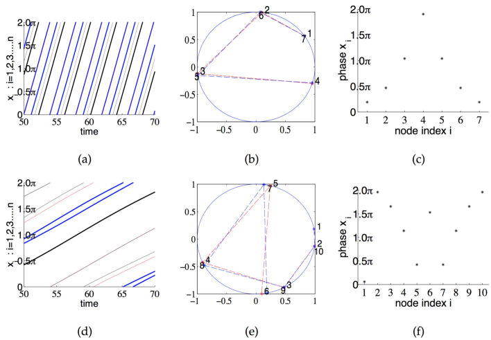
Figure 7: Typical stable special nonlinear waves. (a), (b), (c) plot a special nonlinear wave on the circle network, with $n=7,\,w=0.8,\,\epsilon=0.05,\,d=1,\,p=1$ for Eq. (28) and Eq. (30). (d), (e), (f) plot a special nonlinear wave on the circle network, with $n=10,\,w=0.8,\,\epsilon=0.05,\,d=1,\,p=-1$ for Eq. (29) and Eq. (30). Blue stars in (b) and (e) indicate the corresponding analytical solution with $\epsilon=0$ in Eq. (13).

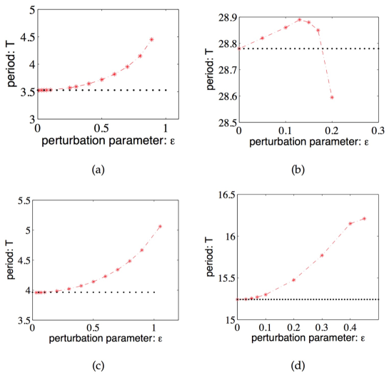
Figure 8: The dependence of the period on $\epsilon$ for different stable special nonlinear waves. Simulation results are plotted as red stars (with dashed line), along with the analytic result for $\epsilon=0$ serving as the baseline, which are plotted as black dots. (a) The parameter values are $n=7,\,w=0.8,\,d=1,\,p=1$ in Eq. (28) and Eq. (30). (b) The same with (a) except that $p=-1$. (c) $n=10,\,w=0.8,\,d=1,\,p=1$ in Eq. (29) and Eq. (30). (d) The same with (c) but $p=-1$.

IV Circulating pulse and regular nonlinear wave

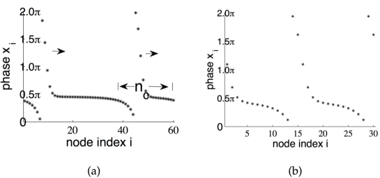
Figure 9: (a) Two independent circulating pulses on a circle network with $n=60,\,w=0.99,\,\epsilon=1,\,d=1$. The moving direction is indicated by the arrow. $n_{c}$ is the number of nodes covered by one pulse. (b) A regular nonlinear wave with $k=2,\,n=30,\,w=0.99,\,\epsilon=1,\,d=1$.

Our model is closely related to the excitable media on a circle. In previous studies, a circulating pulse was rendered unstable and changed to a steady solution upon decreasing the circumference of the ring Courtemanche et al. (1993); Frame and Simson (1988). In our discrete model, pulses would first change to regular nonlinear waves with decreasing $n$. The difference between circulating pulses and regular nonlinear waves are explained in Fig. 9. In Fig. 9(a), the two pulses do not constitute a regular nonlinear wave, since the distance between them may be adjusted freely as long as it is larger than the critical number $n_{c}$, where $n_{c}$ is the number of nodes spanned by a single pulse , thus contradicting the uniqueness of the regular nonlinear wave with $k=2$. Note that the node indices corresponding to peaks are $i_{peak1}=8,i_{peak2}=45$ and thus $i_{peak2}-i_{peak1}\neq n/2=30$, while $i_{peak2}-i_{peak1}=n/2$ for a regular nonlinear wave, as depicted in Fig. 9(b). When $n$ decreases to 30, the two pulses strongly interact with each other and a regular nonlinear wave with $k=2$ emerges. So a circulating pulse can be viewed as a local structure, which spreads over $n_{c}$ nodes in the circle network, as indicated in Fig. 9(a). Two pulses will change to a regular nonlinear wave if they overlap. This phenomenon is characteristic of the discreteness of our model on a circle network.

The circulating pulse is similar to the soliton solution of the Frenkel-Kontorova model. The stability of circulating pulse is due to the excitable property of individual nodes while the stability of soliton is also well explained in the Frenkel-Kontorova model in terms of the lattice pinning effect Braun and Kivshar (2004), i.e., potential well created by the discreteness of lattice. Our model describe the lattice pinning effect and the excitability property in an equivalent and unified way.

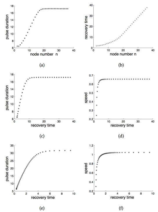
Figure 10: Interesting characterizations of the circulating pulse in a circle network. $d=1,\,\epsilon=1$ in all plots. (a) The pulse duration $a$ as a function of the total node number $n$, with $\omega=0.8$. (b) The recovery time $t_{r}(n)$, with $\omega=0.8$. (c) The restitution curve $a(t_{r})$ with $\omega=0.8$. (d) The dispersion curve $c(t_{r})$ with $\omega=0.8$. (e) The restitution curve $a(t_{r})$ with $\omega=0.99$. (f) The dispersion curve $c(t_{r})$ with $\omega=0.99$.

The recovery time and the pulse duration are two important physical observables in the evolution of excitable node dynamics and have been well characterized in the literature Courtemanche et al. (1993). In our case, the recovery time $t_{r}$ is the time spent in overcoming the barrier between two fixed points defined by the local dynamics (i.e., $x_{fix1}=\arcsin(w),\,x_{fix2}=\pi-\arcsin(w)$). $t_{r}=t_{2}-t_{1}$, where $x(t_{1})=x_{fix1},\,\,x(t_{2})=x_{fix2}$. The pulse duration $a=T-t_{r}$ is the time spent in the long excursion away from the fixed points. Due to the rotational symmetry of our model, $t_{r}$ and $a$ are independent of node position in the circle network, but strongly dependent on the circumference $n$. A careful simulation is undertaken to determine the curves $t_{r}(n),\,a(n),\,a(t_{r}),\,c(t_{r})$, shown in Fig. 10, where $c$ is the speed of the circulating wave defined by $c=n/(t_{r}(n)+a(n))$. The curve $a(t_{r})$ is termed the restitution curve and $c(t_{r})$ the dispersion curve. These curves are important in that they help us understand relevant and universal properties for circulating pulses in a circle network Courtemanche et al. (1993).

In Fig. 10(a) and (b), there is a turning point in $a(n)$ and $t_{r}(n)$ around $n=18$, which signifies a transition from a regular nonlinear wave to a circulating pulse. The saturation in $a(n)$ and the constant slope for $t_{r}(n)$ when $n>18$ is characteristic of a circulating pulse, simply because the pulse does not spread over all nodes and moves at a constant speed along the circle network for $n$ large enough. Thus the critical number $n_{c}$ of nodes covered by a pulse can be defined as $n$ at the transition point. Geometrically, on the phase circle, an increasing number of nodes are moving at the recovery stage with a decreasing speed and thus raised the recovery time. The density of the nodes on the excursion contour remains constant for large $n$, leading to a constant duration time. The restitution curve $a(t_{r})$ and the dispersion curve $c(t_{r})$ are plotted in Fig. 10 with different $\omega$’s which look qualitatively similar. The difference originates from disparate distances between fixed points of the local dynamics. The saturation of $a(t_{r})$ and $c(t_{r})$ are also associated with the transition from a regular nonlinear wave to a pulse. Similar saturation behavior was observed in a one-dimensional ring of excitable media with very sophisticated description of motion dynamics Courtemanche et al. (1993). The physical observables $t_{r}(n),\,a(n),\,a(t_{r}),\,c(t_{r})$ used here are universal quantities for characterizing circulating pulses in a circle network.

V Summary

Previous works Qian et al. (2010) suggest that dynamics of coupled excitable nodes on a complex network may have a very simple yet universal structure, which includes self-sustained oscillation on the circle sub-network and attached branches driven by the center oscillation. This article focuses on discussion on possible solutions for a new type of equation, which is simple enough for analytic computation yet captures the essence of nonlinear wave generation and propagation on networks with excitable nodes. This new model can be viewed as a most direct extension of the Kuramoto model to treat the excitable dynamics, the understanding of which will help us study possible behaviors of other models with excitable dynamics on complex networks due to its universality.

In this paper, we carried out a quite thorough study of the new model on circle networks and reveals certain universality of regular solutions, which is quite independent of the local dynamics and the attached branches being driven, and closely related to the Laplacian coupling of neighboring nodes. Although there are numerous solutions for this system, in terms of stability and basin of attraction, regular nonlinear waves and, in the case of large number of nodes, circulating pulses are the most important solutions, which was confirmed by simulation. The period $T$ for regular nonlinear waves is computed analytically which agrees well with the numerical result up to $\epsilon\sim 0.5\omega$. An analytic form of the regular nonlinear wave is also obtained to the first order. A new type of solution, the special nonlinear wave, is also studied and compared to the regular solution. It is stable under certain parameter regime but only exists in the discrete dynamics. The properties of circulating pulses on circle network with excitable nodes were discussed in detail and its relevance to the regular solution is also studied.

Our model is closely related to the Frenkel-Kontorova model. While the classical Frenkel-Kontorova model describes the Newtonian dynamics of a chain of classical particles, here we use the over-damped version with a special form of coupling and use it to study pattern formation on complex networks. The simplicity of this model and previous understanding of the Frenkel-Kontorova model hopefully give physical insights while still keeping the analytic understanding within reach.

Much more work needs to be done. For example, the existence condition and the basin of attraction for each regular solution should be more precisely characterized. Further, we may employ the current model to study the interaction of the circle sub-network and the attached branches in a network of general topology, or the interaction of real complex networks. It would be interesting to compare wave propagation on the same network but with different excitable dynamics.

Appendix A Stability of solutions

Let us consider the stability of solutions for Eq. (8). We write the perturbation solution in this form $\eta_{i}^{(p)}=\eta_{i}+\epsilon_{i}$, in which $\eta_{i}$ is the stationary solution for Eq. (8) and satisfies Eq. (11). Ignoring higher order terms of $\epsilon$, a substitution of $\eta_{i}^{(p)}$ into Eq. (8) gives

$$\frac{d\epsilon_{i}}{dt}=\alpha(\epsilon_{i+1}+\epsilon_{i-1}-2\epsilon_{i})\,,$$ (31)

where $\alpha=d\cos(\beta)$. Suppose $\alpha>0$, then

$$\frac{d\vec{\epsilon}}{d\tau}=-\alpha Q\vec{\epsilon}=A\vec{\epsilon}\,.$$

So $Q$ can be viewed as a Laplacian matrix of the circle network. It turns out that $Q$ is a positive semi-definite matrix, with eigenvalues $0=\lambda^{\prime}{}_{0}\leq\lambda^{\prime}{}_{1}\leq...\leq\lambda^{\prime}{}_{n-1}$. So the eigenvalues $\lambda_{i}$ for $A=-\alpha Q$ are all non-positive if $\alpha>0$.

More specifically, suppose

$$\epsilon_{i}=ae^{j\frac{2mi\pi}{n}}e^{\lambda_{m}\tau},m=0,1,...n-1\,,$$

where $j=\sqrt{-1}$. Then $\lambda_{m}=-4\alpha\sin^{2}(m\pi/n)$, which are the eigenvalues of this system. All the eigenvectors for $m>0$ correspond to the stable direction and the one for the eigenvalue $\lambda_{0}=0$ corresponds to the rotation of the system as a whole. Therefore, up to a rotation, the solution is stable and the larger $\alpha$ is, the more stable the solution will be. From the discussion above, we conclude that $\alpha>0$ gives stable solutions while $\alpha=0$ neutrally stable solutions and $\alpha<0$ unstable solutions.

However, the following situation

$$\exists\,m,\,\eta_{m+1}-\eta_{m}=\beta\,\,\text{and}\,\eta_{m}-\eta_{m-1}=\pi-\beta$$

for the stationary solution of Eq. (8) is more difficult to analyze. This situation may possibly though not necessarily bring instability to the system. Numerical simulation results show that that the system would be unstable under this condition in most cases except a few.

Appendix B The Poincaré-Lindstedt method

In seeking for a periodic solution, the regular perturbation technique usually fails because the period of the new solution is slightly different from that of the unperturbed one which the perturbation expansion starts from. The mismatch of the two periods usually results in secular terms which grow without bound. The Poincaré-Lindstedt method overcomes this shortcoming by allowing stretching or compressing of the time coordinate, thus matching the two periods. To implement this method, we need to make sure that the periodic solution exists and the expansion converges at least for the small perturbation. Below, we briefly review the theorem on the existence of periodic solutions and then verify that our general model satisfies the existence conditions.

B.1 The existence of periodic solutions

Consider in $\mathbb{R}^{n}$ the equation

$$\dot{x}_{i}=f_{i}(\vec{x})+\epsilon g_{i}(\vec{x})\,,$$ (32)

where $\epsilon$ is a small parameter, $i\in\{1,2,...,n\}$, $\vec{x}=(x_{1},x_{2},...,x_{n})$, $f_{i}(\vec{x})=f_{i}(x_{1},x_{2},...,x_{n})$ and $g_{i}(\vec{x})=g_{i}(x_{1},x_{2},...,x_{n})$. We are seeking the periodic solutions of the equation. For the unperturbed equation

$$\dot{y}_{i}=f_{i}(\vec{y})\,,$$

it is assumed that a $T_{0}$-periodic solution

$$y_{i}=G_{i}(t;\varphi_{1},\varphi_{2},...,\varphi_{n})$$ (33)

exists with $\varphi_{i}$’s being integral constants. To get a periodic solution for Eq. (32), it is convenient to make a coordinate transformation

$$\Omega t=\tau,\,\Omega^{-1}=\omega^{-1}+\epsilon\phi_{0}(\epsilon),$$

with $\Omega$ being the frequency of the new solution and $\omega=2\pi/T_{0}$. This transformation allows us to directly approximate the new period. After this transformation, the new sought solution is $2\pi$-periodic in $\tau$. A perturbation expansion of the solution for Eq. (32) could be written as

$$x_{i}=M_{i}(\tau;\phi_{0},\phi_{1},\phi_{2},...,\phi_{n},\epsilon).$$ (34)

Denote

$$H_{i}(\vec{\phi},\epsilon)=M_{i}(2\pi;\phi_{0},\phi_{1},\phi_{2},...,\phi_{n},\epsilon)-M_{i}(0;\phi_{0},\phi_{1},\phi_{2},...,\phi_{n},\epsilon),$$

where $\vec{\phi}=(\phi_{0},\phi_{1},...,\phi_{n})$. The periodicity condition requires

$$H_{i}(\vec{\phi},\epsilon)=0\,,$$ (35)

which determines $n$ parameters from the $n$ periodicity conditions Eq. (35) in the neighborhood of $\epsilon=0$. The extra parameter corresponds to the time translational symmetry of the autonomous equations. Eq. (35) is equivalent to

$$\text{rank}\Big{(}\frac{\partial\vec{H}}{\partial\vec{\phi}}\Big{)}=n,$$ (36)

where $\vec{H}=(H_{1},H_{2},...,H_{n})^{T}$ and $\frac{\partial\vec{H}}{\partial\vec{\phi}}$ is the Jacobian matrix of $\vec{H}$. This is also called the uniqueness condition since it determines uniquely the new periodic solution up to a time translation.

Below we state theorems relevant to the Poincaré-Lindstedt method. See J.K.Hale (1963)[Chapter 9 and 10] for more details.

The Poincaré expansion theorem addresses the problem of the convergence of the usual perturbation solution of differential equations within certain time scale. And it roughly states that if $f_{i}(\vec{x})$ and $g_{i}(\vec{x})$ of Eq. (32) can be expanded in a convergent power series with respect to $\vec{x}$, then regular perturbation series converge in the neighborhood of $\epsilon=0$ and the original initial condition within a time-scale 1.

The uniqueness theorem of periodic solutions concludes that If the uniqueness condition Eq. (36) is satisfied for Eq. (32), along with the requirement of the Poincaré expansion theorem and the periodicity condition Eq. (35), then there exists a periodic solution which can be represented by a convergent power series in $\epsilon$ in the form of Eq. (34) for $0\leq\epsilon<\epsilon_{0}$ for some positive $\epsilon_{0}$.

B.2 Justification

Now we justify the application of the Poincaré-Lindstedt method in our generalized model Eq. (15), which apparently satisfies the condition of the Poincaré expansion theorem since $g(x),\,h(x)$ are both smooth functions. Below, we check the uniqueness and periodicity conditions.

Under the coordinate transformation

$$\Omega t=\tau,\,\Omega^{-1}=\omega^{-1}+\phi_{0}(\epsilon)\,,$$

where $\phi_{0}(\epsilon)=O(\epsilon)$, Eq. (15) becomes

$$\frac{dx_{i}}{d\tau}=1+\omega\phi_{0}-(\frac{\epsilon}{\omega}+\epsilon\phi_{0})g+(\phi_{0}+\frac{1}{\omega})h.$$ (37)

For the unperturbed equation

$$\frac{dy_{i}}{d\tau}=1+\frac{1}{\omega}h(y_{i+1}+y_{i-1}-2y_{i}),$$

the regular solution is

$$y_{i}(\tau)=\tau-\frac{2(i-1)k\pi}{n}\,.$$

We can express the regular solution for Eq. (37) as

$$\begin{split}&x_{i}(\tau)=\tau-\frac{2(i-1)k\pi}{n}+\phi_{i}+\\ &\int_{0}^{\tau}\Big{(}\omega\phi_{0}-(\frac{\epsilon}{\omega}+\epsilon\phi_{0})g(x_{i}(\theta))+(\phi_{0}+\frac{1}{\omega})h(x_{i+1}(\theta)+x_{i-1}(\theta)-2x_{i}(\theta))\Big{)}d\theta,\end{split}$$ (38)

where $\phi_{i}=O(\epsilon)$ is a constant parameter and $\phi_{i}|_{\epsilon=0}=0$. In accordance with the Poincaré expansion theorem, we assume that

$$y_{i}=x_{i}+O(\epsilon),$$ (39)

then $x_{i+1}(\theta)+x_{i-1}(\theta)-2x_{i}(\theta)\approx O(\epsilon)$, thus

$$h(x_{i+1}+x_{i-1}-2x_{i})=h(0)+h`(0)O(\epsilon)+o(\epsilon)=O(\epsilon).$$

Then

$$\int_{0}^{\tau}\left(\omega\phi_{0}-(\frac{\epsilon}{\omega}+\epsilon\phi_{0})g(x_{i})+(\phi_{0}+\frac{1}{\omega})h(x_{i+1}+x_{i-1}-2x_{i})\right)d\theta=O(\epsilon),$$

which is consistent with Eq. (39). A substitution of $y_{i}$ for $x_{i}$ at the right side of Eq. (37) with the notation $z_{i}=y_{i}+\phi_{i}$ gives

$$x_{i}(\tau)=z_{i}+\int_{0}^{\tau}\left((\omega\phi_{0}-\frac{\epsilon}{\omega}g(z_{i}))+\frac{h`(0)}{\omega}(z_{i+1}+z_{i-1}-2z_{i})\right)d\theta+o(\epsilon).$$ (40)

The periodicity condition is

$$x_{i}(2\pi)=x_{i}(0)+2\pi\,,$$

which, with the notation

$$H_{i}=\int_{0}^{2\pi}\left((\omega\phi_{0}-\frac{\epsilon}{\omega}g(z_{i}))+\frac{h`(0)}{\omega}(z_{i+1}+z_{i-1}-2z_{i})\right)d\theta+o(\epsilon).$$

is equivalent to

$$H_{i}(\phi_{0},\phi_{1},...,\phi_{n})=0,\,i\in\{1,2,...,n\}.$$

Below, we calculate the Jacobian matrix of $\vec{H}$ in the neighborhood of $\epsilon=0$ and $\vec{\phi}=0$, where $\vec{\phi}=(\phi_{0},\phi_{1},...,\phi_{n})$:

$$\frac{\partial H_{i}}{\partial\phi_{0}}=2\pi\omega,\,i\in\{1,2,...,n\}.$$

$$\frac{\partial H_{i}}{\partial\phi_{i}}=\int_{0}^{2\pi}\Big{(}-\frac{g`(z_{i})}{\omega}-2\frac{h`(0)}{\omega}\Big{)}d\theta,\,i\in\{1,2,...,n\}$$

Note that $g$ is a $2\pi$-periodic function, thus

$$\int_{0}^{2\pi}\Big{(}-\frac{g`(z_{i}(\theta))}{\omega}d\theta\Big{)}=\int_{z_{i}(0)}^{z_{i}(0)+2\pi}\Big{(}-\frac{g`(z_{i}(\theta))}{\omega}dz_{i}\Big{)}=-\frac{g(z_{i}(0)+2\pi)-g(z_{i}(0))}{\omega}=0.$$

Then

$$\frac{\partial H_{i}}{\partial\phi_{i}}=-2\frac{2\pi h`(0)}{\omega},\,i\in\{1,2,...,n\}.$$

Besides,

$$\frac{\partial H_{i}}{\partial\phi_{m}}=\frac{2\pi h`(0)}{\omega}(\delta(m-i-1)+\delta(m-i+1)),$$

where $m,i\in\{1,2,...,n\}$, $m\neq i$ and

$$\delta(s)=\begin{cases}1,&\quad s=0\\ 0,&\quad s\neq 0.\end{cases}$$

Finally, we obtain the Jacobian matrix for $\vec{H}$

$$\frac{\partial\vec{H}}{\partial\vec{\phi}}=\frac{2\pi h`(0)}{\omega}\begin{bmatrix}a&-2&1&&&&1\\ a&1&-2&1&&&\\ a&&1&-2&1&&\\ \vdots&&&\ddots&\ddots&\ddots&\\ a&&&&1&-2&1\\ a&1&&&&1&-2\end{bmatrix},$$ (41)

where $a=\frac{\omega^{2}}{h`(0)}$. This is an $n\times(n+1)$ matrix with $n$ linearly independent column vectors, thus

$$\text{rank}\Big{(}\frac{\partial\vec{H}}{\partial\vec{\phi}}\Big{)}=n\,,$$

which is just what the uniqueness condition requires for the existence of periodic solutions. According to the theorem of existence of periodic solutions, periodic solutions exist in our general model and the Poincaré-Lindstedt method can be applied.

Appendix C Response to spatiotemporally periodic driving force

On a circle network, with diffusive coupling and subject to a spatiotemporal periodic driving, the equation of motion has the form

$$\dot{f_{i}}=F(i,t)+d(f_{i-1}+f_{i+1}-2f_{i})\,,$$ (42)

where $F(i,t)=F(i+n,t)=F(i,t+T)$ with $n$ being the number of nodes and $T$ the period of the driving. With some minor assumptions, a periodic solution to this equation would be stable if $d>0$, because the linearized equation takes the form of Eq. (31). In the following, we are mainly interested in the type of equations that are relevant to the proof in section III.2.

Firstly, consider

$$F(i,t)=a\exp\left(j\Big{(}mt-\frac{(i-1)2km\pi}{n}\Big{)}\right)\,,$$

where $j$ is the imaginary number unit. Suppose the solution takes the form

$$f_{i}(t)=A\exp\left(j\Big{(}mt-m(i-1)2k\pi/n\Big{)}\right)\,,$$ (43)

and substituting it into Eq. (42) results in

$$A=\frac{a}{jm+4d\sin^{2}(\frac{mk\pi}{n})}\,.$$

With this basic solution, we can easily calculate solutions for other types of driving terms. Consider

$$F(i,t)=a\sin\Big{(}mt-\frac{(i-1)m2k\pi}{n}\Big{)}\,.$$ (44)

An implementation of Eq. (43) leads to

$$\begin{split}f_{i}(t)=&\frac{4ad\sin^{2}(mk\pi/n)}{m^{2}+(4d\sin^{2}(mk\pi/n))^{2}}\sin\Big{(}mt-\frac{m(i-1)2k\pi}{n}\Big{)}\\ &-\frac{am}{m^{2}+(4d\sin^{2}(mk\pi/n))^{2}}\cos\Big{(}mt-\frac{m(i-1)2k\pi}{n}\Big{)}\,.\end{split}$$ (45)

The cosine driving

$$F(i,t)=a\cos\Big{(}mt-\frac{(i-1)2mk\pi}{n}\Big{)}\,,$$

gives then

$$\begin{split}f_{i}(t)=&\frac{am}{m^{2}+(4d\sin^{2}(mk\pi/n))^{2}}\sin\Big{(}mt-\frac{m(i-1)2k\pi}{n}\Big{)}\\ &+\frac{4ad\sin^{2}(mk\pi/n)}{m^{2}+(4d\sin^{2}(mk\pi/n))^{2}}\cos\Big{(}mt-\frac{m(i-1)2k\pi}{n}\Big{)}\,.\end{split}$$ (46)

All the solutions obtained above are stable nonlinear waves on the circle network, driven by spatiotemporally periodic force.

References

- Peskin (1975) C. Peskin, Mathematical aspects of heart physiology (Courant Institute of Mathematical Sciences, New York, 1975).
- Michaels et al. (1987) D. Michaels, E. Matyas, and J. Jalife, Circ. Res. 61, 704 (1987).
- Ghosh et al. (1971) A. Ghosh, B. Chance, and E. Pye, Arch. Biochem. Biophys. 145, 319 (1971).
- Aldridge et al. (1976) J. Aldridge, E. Pye, et al., Nature 259, 670 (1976).
- Buck (1988) J. Buck, Quart. Rev. Biol 63, 265 (1988).
- Buck and Buck (1976) J. Buck and E. Buck, Sci. Am. 234, 74 (1976).
- Jiang and McCall (1993) Z. Jiang and M. McCall, JOSA B 10, 155 (1993).
- Kourtchatov et al. (1995) S. Kourtchatov, V. Likhanskii, A. Napartovich, F. Arecchi, and A. Lapucci, Phys. Rev. A 52, 4089 (1995).
- York and Compton (1991) R. York and R. Compton, IEEE T. Microw. Theory 39, 1000 (1991).
- Wiesenfeld et al. (1996) K. Wiesenfeld, P. Colet, and S. Strogatz, Phys. Rev. Lett. 76, 404 (1996).
- Acebrón et al. (2005) J. Acebrón, L. Bonilla, C. Vicente, F. Ritort, and R. Spigler, Rev. Mod. Phys. 77, 137 (2005).
- Hong et al. (2007) H. Hong, H. Park, and L. Tang, Phys. Rev. E 76, 066104 (2007).
- Arenas et al. (2008) A. Arenas, A. Díaz-Guilera, J. Kurths, Y. Moreno, and C. Zhou, Phys. Rep. 469, 93 (2008).
- Qian et al. (2010) Y. Qian, X. Huang, G. Hu, and X. Liao, Phys. Rev. E 81, 036101 (2010).
- Frame and Simson (1988) L. Frame and M. Simson, Circulation 78, 1277 (1988).
- Courtemanche et al. (1993) M. Courtemanche, L. Glass, and J. P. Keener, Phys. Rev. Lett. 70, 2182 (1993).
- Grüner et al. (1989) G. Grüner et al., Charge density waves in solids, vol. 25 (North Holland, Amsterdam, 1989).
- Rosenblum et al. (1997) M. Rosenblum, A. Pikovsky, and J. Kurths, Phys. Rev. Lett. 78, 4193 (1997).
- Chenciner and Montgomery (2000) A. Chenciner and R. Montgomery, Ann. Math. 152, 881 (2000).
- Braun and Kivshar (2004) O. Braun and Y. Kivshar, The Frenkel-Kontorova model: concepts, methods, and applications (Springer, New York, 2004).
- Aubry and Le Daeron (1983) S. Aubry and P. Le Daeron, Physica D 8, 381 (1983).
- Bak (1982) P. Bak, Rep. Prog. Phys. 45, 587 (1982).
- Bär and Eiswirth (1993) M. Bär and M. Eiswirth, Phys. Rev. E 48, R1635 (1993).
- Ermentrout and Kopell (1986) G. Ermentrout and N. Kopell, SIAM J. Appl. Math. 46, 233 (1986).
- Wiesenfeld et al. (1998) K. Wiesenfeld, P. Colet, and S. Strogatz, Physical Review E 57, 1563 (1998).
- Middleton (1992) A. Middleton, Phys. Rev. Lett. 68, 670 (1992).
- Pietronero and Strässler (1983) L. Pietronero and S. Strässler, Phys. Rev. B 28, 5863 (1983).
- Matsukawa and Takayama (1984) H. Matsukawa and H. Takayama, Solid State commun. 50, 283 (1984).
- Strogatz et al. (1988) S. Strogatz, C. Marcus, R. Westervelt, and R. Mirollo, Phys. Rev. Lett. 61, 2380 (1988).
- Verhulst (1996) F. Verhulst, Nonlinear differential equations and dynamical systems (Springer, New York, 1996).
- J.K.Hale (1963) J.K.Hale, Oscillations in nonlinear systems (McGraw-Hill, New York, 1963).