Joint Crosstalk-Avoidance and Error-Correction Coding for Parallel Data Buses

Abstract

Decreasing transistor sizes and lower voltage swings cause two distinct problems for communication in integrated circuits. First, decreasing inter-wire spacing increases interline capacitive coupling, which adversely affects transmission energy and delay. Second, lower voltage swings render the transmission susceptible to various noise sources. Coding can be used to address both these problems. So-called crosstalk-avoidance codes mitigate capacitive coupling, and traditional error-correction codes introduce resilience against channel errors.

Unfortunately, crosstalk-avoidance and error-correction codes cannot be combined in a straightforward manner. On the one hand, crosstalk-avoidance encoding followed by error-correction encoding destroys the crosstalk-avoidance property. On the other hand, error-correction encoding followed by crosstalk-avoidance encoding causes the crosstalk-avoidance decoder to fail in the presence of errors. Existing approaches circumvent this difficulty by using additional bus wires to protect the parities generated from the output of the error-correction encoder, and are therefore inefficient.

In this work we propose a novel joint crosstalk-avoidance and error-correction coding and decoding scheme that provides higher bus transmission rates compared to existing approaches. Our joint approach carefully embeds the parities such that the crosstalk-avoidance property is preserved. We analyze the rate and minimum distance of the proposed scheme. We also provide a density evolution analysis and predict iterative decoding thresholds for reliable communication under random bus erasures. This density evolution analysis is nonstandard, since the crosstalk-avoidance constraints are inherently nonlinear.

I Introduction

I-A Motivation and Related Work

The various components in an integrated circuit communicate with each other via parallel metal wires referred to as interconnects or parallel buses [1, 2, 3, 4]. As the inter-wire spacing decreases with technology scaling, the coupling capacitance between adjacent wires increases, leading to increased crosstalk on the bus [5]. Moreover, scaling of the supply voltage renders bus transmissions susceptible to random errors. Together, these two effects increase transmission energy/delay and degrade signal integrity. As a consequence, they pose a major challenge to keep up with the demand for increasing data transfer rates over interconnects.

Crosstalk-avoidance coding (CAC) encodes data for transmission over a capacitively-coupled interconnect with reduced energy consumption and propagation delay. This is achieved, for example, by avoiding opposing bit transitions on adjacent bus wires [5, 6, 7, 8].

Error-correction coding (ECC) encodes data by adding redundancy in the form of parity bits. This redundancy can then be used to detect and correct errors occurring during the transmission. Such error correction is becoming increasingly important for communication over interconnects. For example, the DDR4 SDRAM standard uses an $8$-bit cyclic-redundancy code to provide error correction for $72$ bits of data transmitted over the bus [9]. Thus, the total number of bus wires used is $80$.

Since parallel buses benefit from the use of both CAC and ECC, it is beneficial to try to combine them. However, this turns out to be nontrivial. The two natural approaches, which use an ECC inner code followed by a CAC outer code, or which use a CAC inner code followed by an ECC outer code both fail (the former because the CAC outer code cannot be reliably decoded in the presence of errors, the latter since the ECC outer code destroys the crosstalk-avoidance property). Thus, crosstalk-avoidance and error-correction coding need to be performed jointly.

The best known way to combine CAC and ECC is [10, 11]. They propose to first encode the information using a CAC. Next an ECC is used to generate parity bits for the output of the CAC. Each of these parity bits is transmitted using two wires to ensure crosstalk avoidance. As a result of this duplication, this approach is inefficient. For example, using the above DDR4 numbers, if the $72$ bits are already CAC encoded, then the ECC would generate an additional $16$ bits to carry the $8$ parity bits, resulting in a total of $88$ bus wires.

I-B Summary of Contributions

We propose an efficient method to perform joint CAC and ECC that uses fewer bus wires than the state-of-the-art [10] and in addition can provide better error correction. For the DDR4 example above, our proposed scheme for joint CAC and ECC uses only an additional $10$ bits to carry the $8$ parity bits, resulting in a total of $82$ bus wires. This constitutes a savings of $6$ bus wires over the state of the art [10].

The key ingredient in our approach for joint CAC and ECC is to identify what we term free wires. These are wires that can carry either a $0$ or a $1$ without violating the crosstalk-avoidance constraints and without influencing what can be sent over adjacent bus wires. Suppose that there are $P$ such free wires. Our joint CAC and ECC then operates as follows. We first encode the information bits using a CAC to form $N-P$ encoded bits, skipping the free wires during the encoding. We next generate $P$ parity bits for the $N-P$ CAC-encoded bits using an ECC. We finally place the $P$ parity bits on the free wires identified earlier. Notice that, by placing the parity bits on the free wires, they automatically satisfy the CAC constraints, and hence we do not need to duplicate or otherwise shield them in order to protect them against crosstalk as done in [10]. In other words, the parities are embedded into the bits to be transmitted.

We point out that identification of the free wires is possible knowing only the past bus state. Hence, the receiver can correctly determine which wires carry the parity bits. Once the receiver knows the location of the parity bits, it can decode the ECC and CAC. Here, we perform the ECC and CAC decoding jointly. This joint decoding allows us to obtain better error correction than the approach proposed in [10], which decodes the ECC and CAC separately. In this paper we use an irregular repeat-accumulate (IRA) code [12] as our choice of ECC. Since both the ECC and CAC employ local constraints we apply a modified iterative belief-propagation decoder [13] to jointly decode the transmitted codeword.

In summary, the proposed method has two benefits over the state-of-the-art [10]. First, our joint CAC-ECC encoding scheme at the transmitter, by identifying free wires, uses fewer bus wires for transmission of data for the same number of parity bits. Second, the joint CAC-ECC iterative decoding scheme at the receiver allows for better error correction.

We provide a performance analysis for our proposed joint CAC-ECC scheme by computing its rate, minimum distance, and iterative decoding threshold in presence of random erasures. The factor graph [14] for our joint scheme consists of both linear (ECC) and nonlinear (CAC) factor nodes. Hence, the density evolution analysis is nonstandard and we believe this itself is an interesting aspect of our work.

I-C Organization

The remainder of this paper is organized as follows. Section II provides background material on crosstalk-avoidance coding. Section III introduces the joint embedded CAC-ECC code. Sections IV and V analyze the proposed joint embedded CAC-ECC code, evaluating its rate, minimum distance, and iterative decoding thresholds. The proofs of various statements are deferred to the appendices.

II Background on Crosstalk-Avoidance Codes

This section provides some background material on crosstalk-avoidance coding. As mentioned earlier, due to capacitative coupling of adjacent bus wires, certain bus transitions lead to longer transmission delays and higher energy consumption than others [5]. This effect is particularly pronounced for opposing transitions on adjacent wires, i.e., a first wire transitioning up (from $0$ to $1$) and an immediately adjacent wire transitioning down (from $1$ to $0$). Crosstalk-avoidance codes encode the data to be transmitted over the bus to avoid these opposing transitions on adjacent wires. This encoding reduces the transmission delay and energy by up to a factor $1/2$ depending on the coupling coefficient at the cost of also reducing the data rate [5, 15, 16].

The analysis of such codes was pioneered in [6]. Consider a bus with $N$ wires. Denote by $\bm{a}=(a_{1},a_{2},\dots,a_{N})\in\{0,1\}^{N}$ the past bus state. We are interested in the number of sequences $\bm{b}\in\{0,1\}^{N}$ describing the next bus state that satisfy the crosstalk-avoidance constraint with respect to $\bm{a}$. Clearly, the number of such sequences depends on the past bus state $\bm{a}$. The best case is if $\bm{a}$ is either equal to all ones or all zeros. Then, there can be no opposing transitions on adjacent wires no matter what $\bm{b}$ is, and therefore the number of sequences $\bm{b}$ satisfying the CAC constraints is $2^{N}$. The worst case turns out to be if $\bm{a}$ is an alternating run of 0 and 1, i.e., $0101\dots$ or $1010\dots$, in which case the number of sequences $\bm{b}$ satisfying the CAC constraints is $F(N+2)$, where $F(\cdot)$ denotes the Fibonacci numbers [6].

Alternating runs in $\bm{a}$ turn out to be crucial for the rate and decoder analysis. Consider a past bus state $\bm{a}$ consisting of two alternating runs, e.g., $\dots 01011010\dots$, and assume the first such alternating run has length $d_{1}$ and the second one $d_{2}$. Note that the boundary of the two alternating runs is either $11$ or $00$. Hence, there can be no opposing transition regardless of the value of $\bm{b}$ between those two positions. More precisely, if $\bm{b}_{1}$ and $\bm{b}_{2}$ denote any two vectors of $d_{1}$ and $d_{2}$ bits, respectively, that satisfy the constraints imposed by the first and second alternating runs, then the concatenation $\bm{b}$ of $\bm{b}_{1}$ and $\bm{b}_{2}$ is a vector of length $d_{1}+d_{2}$ that satisfies the constraints imposed by the whole vector $\bm{a}$. Thus, the boundary between alternating runs decouples the problem of how to choose $\bm{b}$ into two noninteracting subproblems of choosing the first $d_{1}$ bits and the second $d_{2}$ bits of $\bm{b}$. Consequently, the number of possible $\bm{b}$ sequences is $F(d_{1}+2)F(d_{2}+2)$ [6].

In general, assume $\bm{a}$ is (uniquely) parsed into maximal alternating runs of lengths $\{d_{m}\}_{m=1}^{M}$. Then the number of possible $\bm{b}$ sequences is $\prod_{m=1}^{M}F(d_{m}+2)$ [6]. The rate $R_{\mathsf{CAC}}(\bm{a})$ of the CAC code with past bus state $\bm{a}$ is thus given by

$$R_{\mathsf{CAC}}(\bm{a})=\frac{1}{N}\sum_{m=1}^{M}\log F(d_{m}+2).$$ (1)

For past bus state $\bm{a}$ generated uniformly at random over $\{0,1\}^{N}$, it is not hard to show that the expected number of alternating runs of degree $d$ is $N2^{-d-1}(1+o(1))$ asymptotically as $N\to\infty$ and that the actual number of alternating runs concentrates around this distribution. Thus, for this random choice of $\bm{a}$, the CAC has asymptotic rate

$$R_{\mathsf{CAC}}(\bm{a})=\sum_{d=1}^{\infty}2^{-d-1}\log F(d+2)\approx 0.824$$

with high probability as $N\to\infty$.

III Embedded Joint CAC-ECC Coding Scheme

In this section we introduce our embedded joint CAC and ECC scheme. One of the key concepts for this scheme are what we term free wires, which are introduced in Section III-A. The encoder and decoder operation are described in Sections III-B and III-C.

III-A Free Wires

Assume as before that the bus has $N$ wires and that the past bus state is $\bm{a}=(a_{1},a_{2},\dots,a_{N})$. We want to set the bus to its next state, denoted again by $\bm{b}=(b_{1},b_{2},\dots,b_{N})$. A wire $n$ such that all the three wires, $a_{n-1}$, $a_{n}$ and $a_{n+1}$ have the same value is called a free wire. For such a free wire, we can set the next value $b_{n}$ to be either $0$ or $1$ without violating the crosstalk constraints and without affecting the values $b_{n-1}$, $b_{n+1}$ that can be sent over the two adjacent wires.

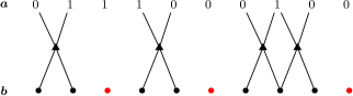
Figure 1: Factor graph depicting free wires (drawn in red). $\bm{a}$ and $\bm{b}$ are the past and future bus state, respectively.

The identification of the free wires is best understood using a factor graph [14] as shown in Fig. 1. On the top in the figure we show the past bus state $\bm{a}$, and on the bottom we show the next bus state $\bm{b}$. The wires in the next bus state $\bm{b}$ are denoted by filled circles. The triangles in the middle represent the crosstalk-avoidance constraints imposed by the past bus state $\bm{a}$. For example, $(a_{1},a_{2})=(0,1)$ requires that $(b_{1},b_{2})\neq(1,0)$ since otherwise we would have an opposing transition on these two adjacent wires.

Notice that there are some values of $\bm{b}$ that are not connected to any constraint. In Fig. 1, the wires $b_{3}$, $b_{6}$, $b_{10}$ (indicated by red filled circles) do not have any constraints associated with them. These are the free wires. Thus, the wires $b_{3}$, $b_{6}$, $b_{10}$ can be set to any value without affecting adjacent wires and without violating any crosstalk constraints. Note that the crosstalk constraints are local: each constraint is connected to two wires of the past bus state and two wires of the next bus state. We also emphasize that the crosstalk constraints are nonlinear, since only one out of four possible values of two adjacent wires is prohibited.

III-B Encoder

Figure 2: Embedded joint CAC-ECC encoder proposed in this paper.

The encoder architecture is shown in Fig. 2. Given the past state $\bm{a}$, the encoder first determines the positions of the free wires. The information bits are passed through the CAC and placed on the non-free wires. The ECC, assumed to be a linear code here and throughout, then computes the parity bits of the data placed on the non-free wires and places them on the free wires.

More formally, let us assume for the moment that the number of free wires is exactly equal to the desired number of parity bits. Then, as shown in the Fig. 2, the encoder first identifies the $P$ free wires. The $K$ information bits are encoded using a CAC and are placed on the $N-P$ non-free wires. The $N-P$ CAC-encoded bits are then fed to the ECC, which generates $P$ parity bits. These parities are then placed on the $P$ free wires. The combined $N-P$ CAC-encoded bits and the generated $P$ parities are sent across the bus.

If the number of free wires is more than the number of parity bits, then the selector uses some of the free wires to carry CAC-encoded information bits. If the number of free wires is less than the number of parity bits, then parity bits are forced on the non-free wires by appropriately shielding them.

In practice, the channel typically operates at very high SNR, and hence we can restrict ourselves to high-rate ECCs, so that the number of parity bits is small. We will show later that when the past bus state $\bm{a}$ is generated uniformly at random from $\{0,1\}^{N}$, then the number of free wires is typically much larger than the desired number of parity bits. Thus, the shielding technique would be rarely used, and our scheme will be efficient most of the time.

So far, we have made no assumptions about the ECC being used except for linearity. To keep decoding complexity manageable, we would like to use a low-density ECC. However, a standard low-density parity-check (LDPC) code cannot be directly combined with the architecture described here since the resulting code will not have vanishing probability of block error. Instead, we propose to use an IRA code [12], in which the parities are further accumulated.

Figure 3: Factor graph for joint embedded CAC and ECC. For clarity, the parity bits are shown separately from the (CAC encoded) information bits. Both of them together represent the $\bm{b}$ vector of bits to be transmitted over the bus.

An example of the factor graph for this construction is shown in Fig. 3. In this figure, the parity-check constraints of the ECC are shown by black squares. An edge between a parity-check constraint and a wire in the next bus state denotes the participation of the bit (on that wire) in that parity-check constraint. The edges associated to the past bus state $\bm{a}$ are half-edges, describing the (fixed and known) bits in the past bus state.

III-C Decoder

To explain the receiver operation we assume that the past bus state $\bm{a}$ is known correctly at the receiver. This allows the receiver to determine the position and number of free wires. We explain only the case when the number of free wires is exactly equal to the number of parity bits. The other cases follow in a similar fashion. The receiver performs a joint iterative decoding of the CAC and ECC to reliably recover the information bits.

Consider the joint factor graph shown in Fig. 3. The goal of the decoder is to determine the information bits in $\bm{b}$ given the noise-corrupted bus output. We will use a modified belief-propagation decoder, which passes messages along the joint factor graph. This modification is needed to take the nonlinear CAC constraints into account. Joint decoding of the CAC and ECC has the advantage that it provides additional error correction compared to the standard approach of only using the ECC for error correction. Indeed, the CAC part of the factor graph provides extrinsic information that can be used by the message-passing decoder.

The $N$ bits in $\bm{b}$, encoded as mentioned above, are transmitted over the bus and face random erasures. The input of the decoder is an $N$-tuple with each entry in $\{0,1,?\}$, where we use $?$ to denote erasures, describing the output of the bus. The decoder is best explained in the language of the joint factor graph consisting of various nodes (cf. Fig. 3). We refer to the wires in the bus, over which the CAC encoded information bits are sent, as the information variable nodes of the factor graph. The parity-bits of the IRA are called parity variable nodes. The CAC and ECC constraints are called CAC-check and ECC-check nodes, respectively. We consider the following message updates at the different nodes in the factor graph.

• Information and parity variable-node updates: Send an erasure message on an outgoing edge if all the incoming messages (including the channel value) are erasures, otherwise send the value (either $0$ or $1$) of the non-erased incoming message.

• CAC node update: Each CAC-constraint node has degree two (cf. Fig. 3) and has two bits of the past bus state as other inputs through half-edges. We distinguish the two (full) edges, connecting the current bus state, by calling them left edge and right edge, respectively. Let us assume for the moment that the past bus state for that constraint node is $(0,1)$ (see the first CAC constraint in Fig. 3). If the incoming message on the left edge is $1$, then the outgoing message on the right edge is set to $1$ because the CAC constraint prohibits the value $(1,0)$ in the current bus state. Otherwise, the outgoing message on the right edge is set to $?$. If the incoming message on the left edge is $0$, then the outgoing message on the right edge is set to $0$ again because the CAC constraint prohibits the value $(1,0)$ in the current bus state. Otherwise the outgoing message on the left edge is set to $?$. The CAC-update rule is analogous for past bus state $(1,0)$.

• ECC check node update: An outgoing message is a non-erasure (either $0$ or $1$) only if all the incoming messages are non-erased, in which case the outgoing message is set to be the XOR of the incoming messages. Otherwise, the outgoing message is set to $?$.

We use the following decoding schedule:

1. Send messages from the information variable nodes to the CAC check nodes.

2. Send messages from the CAC check nodes to the information variable nodes.

3. Send messages from the information variable nodes to the ECC check nodes.

4. Send messages between the ECC check nodes and the parity variable nodes until the messages converge on the accumulate chain.

5. Send messages from the ECC check nodes to the information variable nodes.

This process is repeated until all messages on all edges converge. Initially, the messages sent from the variable nodes to the CAC check nodes are the channel observations. The final value of an information variable node is declared to be an erasure if the incoming messages on all the edges connected to that node are in erasure, otherwise it is set to the value of any non-erased incoming message.

IV Rate and Minimum-Distance Analysis

We begin with the computation of the rate of our embedded joint CAC and ECC scheme. We will compare this with the rate for the shielded joint CAC and ECC from [10]. We next analyze the minimum distance of the proposed embedded joint CAC and ECC scheme. All the results in this section pertain to arbitrary linear ECCs (not necessarily IRA codes).

IV-A Rate

Recall from (1) that $R_{\mathsf{CAC}}(\bm{a})$ denotes the rate of the single CAC for past bus state $\bm{a}$. We also denote by $R_{\mathsf{ECC}}$ the rate of the single ECC. The next theorem provides the rate of the shielded CAC-ECC encoder from [10].

Theorem 1.

The rate $R_{\mathsf{S}}(\bm{a})$ of the shielded joint CAC-ECC encoder from [10] is

$$R_{\mathsf{S}}(\bm{a})=R_{\mathsf{CAC}}(\bm{a})\bigl{(}2R_{\mathsf{ECC}}^{-1}-1\bigr{)}^{-1}.$$

The rate for the proposed embedded joint CAC and ECC scheme is given by the following theorem.

Theorem 2.

Assume that the past bus state $\bm{a}$ has sufficient number of free wires to carry all ECC parities. Then the rate $R_{\mathsf{E}}(\bm{a})$ of the embedded joint CAC-ECC encoder proposed in this paper is

$$R_{\mathsf{E}}(\bm{a})=R_{\mathsf{CAC}}(\bm{a})+R_{\mathsf{ECC}}-1.$$

The proofs of Theorems 1 and 2 are provided in Appendices A and B. We can now compare the two rate expressions

$$R_{\mathsf{S}}(\bm{a}) =R_{\mathsf{CAC}}(\bm{a})\bigl{(}2R_{\mathsf{ECC}}^{-1}-1\bigr{)}^{-1},$$

$$R_{\mathsf{E}}(\bm{a}) =R_{\mathsf{CAC}}(\bm{a})+R_{\mathsf{ECC}}-1,$$

for the shielded and the embedded joint CAC-ECC schemes. We start with a numerical example from the DDR4 SDRAM standard [9].

Example 1.

The DDR4 interconnect communication standard uses a rate $R_{\mathsf{ECC}}=0.9$ cyclic-redundancy check ECC. Assuming the past bus state $\bm{a}$ is generated uniformly over $\{0,1\}^{N}$, the CAC rate is approximately $R_{\mathsf{CAC}}(\bm{a})\approx 0.824$ with high probability for large enough $N$ (cf. Section II). Hence,

$$R_{\mathsf{S}}(\bm{a}) \approx 0.674,$$

$$R_{\mathsf{E}}(\bm{a}) \approx 0.724.$$

Assume we want to transmit $59$ data bits (resulting in $\lceil{59/R_{\mathsf{CAC}}(\bm{a})}\rceil=72$ CAC encoded bits as mentioned in Section I). The shielded joint CAC-ECC encoder from [10] requires $\lceil{59/R_{\mathsf{S}}(\bm{a})}\rceil=88$ wires. The embedded joint CAC-ECC encoder proposed here requires only $\lceil{59/R_{\mathsf{E}}(\bm{a})}\rceil=82$ wires, thereby saving $6$ wires for the same number of parity bits conveyed. ∎

As can be seen from this example, the regime of practical interest is when the error correction code has rate $R_{\mathsf{ECC}}$ close to one. Assume then that $R_{\mathsf{ECC}}=1-\delta$ for some small $\delta>0$. Then,

$$R_{\mathsf{S}}(\bm{a}) =R_{\mathsf{CAC}}(\bm{a})\frac{1-\delta}{1+\delta}$$

$$\approx R_{\mathsf{CAC}}(\bm{a})(1-2\delta)$$

$$=R_{\mathsf{CAC}}(\bm{a})-2R_{\mathsf{CAC}}(\bm{a})\delta.$$

$$R_{\mathsf{E}}(\bm{a}) =R_{\mathsf{CAC}}(\bm{a})-\delta.$$

For a concrete example, assume again that $\bm{a}$ is generated uniformly over $\{0,1\}^{N}$ so that $R_{\mathsf{CAC}}(\bm{a})\approx 0.824$ with high probability for large enough $N$. Then the embedded approach proposed here outperforms the shielded approach from [10] by approximately $0.648\delta$ (as long as it has sufficient free wires to hold the parities for the embedding which is the case with high probability when $\delta<1/4$).

More generally, it can be shown that $R_{\mathsf{E}}(\bm{a})\geq R_{\mathsf{S}}(\bm{a})$ for any past bus state $\bm{a}$ with sufficient number of free wires. Thus, the proposed embedded joint CAC-ECC scheme always outperforms the shielded joint CAC-ECC scheme from [10]. The proof of this fact is reported in Appendix C.

IV-B Minimum Distance

Denote by $d_{\mathsf{ECC}}$ the minimum distance of the ECC. The next theorem shows that the minimum distance of the embedded joint CAC-ECC code is the same as that of the ECC alone.

Theorem 3.

Assume that the past bus state $\bm{a}$ has sufficient number of free wires to carry all ECC parities. Then the minimum distance $d_{\mathsf{E}}(\bm{a})$ of the embedded joint CAC-ECC encoder is

$$d_{\mathsf{E}}(\bm{a})=d_{\mathsf{ECC}}.$$

The proof of Theorem 3 is reported in Appendix D. The theorem shows that joint CAC-ECC encoding does not increase minimum distance. In other words, the additional redundancy introduced by the CAC requirement does not translate into increased minimum distance. This is, of course, somewhat disappointing. However, as we will see in the next section, the CAC redundancy is nonetheless beneficial for error correction, since it does increase the iterative decoding threshold.

V Iterative Decoding Threshold

In this section we will assume that the ECC is an IRA code as described in Section III-B. We perform a density evolution analysis [13, 17, 18] of the iterative decoder described in Section III-C. This analysis allows us to predict the performance of our embedded encoding scheme in the presence of random erasures. We begin in Section V-A by formally introducing the ensembles over which the analysis is performed. The casual reader may wish to skip this section and proceed directly to Section V-B, which reports the density evolution analysis.

V-A Ensembles

Density evolution is an average analysis and predicts the probability of error when averaged over an ensemble of codes. We next describe the ensemble of codes with the help of Fig. 3 in Section III-B.

V-A1 Ensemble of Past Bus States

We start with the probabilistic description of the past bus state $\bm{a}$. A natural assumption would be that $\bm{a}$ is generated uniformly at random from $\{0,1\}^{N}$. As we have seen in Section II, with this assumption the expected number of alternating runs in $\bm{a}$ of length $d$ is asymptotically $N2^{-d-1}$. Unfortunately, this assumption results in a cumbersome analysis, and we instead adopt a modified assumption on the generation of $\bm{a}$ that is easier to handle and asymptotically equivalent as $N\to\infty$.

Recall that the past state $\bm{a}$ can be thought of as a collection of alternating runs of various lengths, with free wires being alternating runs of length one. In our modified assumption, we will generate $\bm{a}$ as the concatenation of independently generated such alternating runs of random length.

Fix the rate for the ECC to be $R_{\mathsf{ECC}}\in(3/4,1]$. Generate $\bm{a}$ as two different parts $\bm{a}_{1}$ and $\bm{a}_{2}$. The first part consists of $N(R_{\mathsf{ECC}}-1/2)$ independently generated alternating runs. Each such alternating run has random length $D$ with identical probability given by

$$\mathbb{P}(D=d)\mathrel{\triangleq}\begin{cases}\frac{2R_{\mathsf{ECC}}-3/2}{2R_{\mathsf{ECC}}-1},&\text{for $d=1$},\\ \frac{2^{-d}}{2R_{\mathsf{ECC}}-1},&\text{for $d\in\{2,3,\dots\}$}.\end{cases}$$

Let $\ell(\bm{a}_{1})$ be the length of this first part. The expected value of this length is

$$N(R_{\mathsf{ECC}}-1/2)\sum_{d=1}^{\infty}d\mathbb{P}(D=d)=\frac{N(R_{\mathsf{ECC}}-1/2)}{2R_{\mathsf{ECC}}-1}\biggl{(}2R_{\mathsf{ECC}}-3/2+\sum_{d=2}^{\infty}d2^{-d}\biggr{)}=NR_{\mathsf{ECC}}.$$

The bits in $\bm{b}$ corresponding to $\bm{a}_{1}$ will be used to carry the CAC encoded information bits.

The second part $\bm{a}_{2}$ is generated as $\ell(\bm{a}_{1})(1-R_{\mathsf{ECC}})/R_{\mathsf{ECC}}$ alternating runs of length one. Thus, the length $\ell(\bm{a}_{2})$ of this second part is

$$\ell(\bm{a}_{2})=\ell(\bm{a}_{1})(1-R_{\mathsf{ECC}})/R_{\mathsf{ECC}}$$ (2)

and has expected value

$$NR_{\mathsf{ECC}}(1-R_{\mathsf{ECC}})/R_{\mathsf{ECC}}=N(1-R_{\mathsf{ECC}}).$$

The bits in $\bm{b}$ corresponding to $\bm{a}_{2}$ will be used to carry the accumulated parity bits.

We generate the complete past bus state $\bm{a}$ by randomly interleaving the alternating runs in $\bm{a}_{1}$ and in $\bm{a}_{2}$, i.e., with uniform distribution over all possible interleavings of the corresponding runs. The past state $\bm{a}$ has thus expected length

$$NR_{\mathsf{ECC}}+N(1-R_{\mathsf{ECC}})=N$$

as required.

We also point out that the expected number of alternating runs in $\bm{a}$ of degree $d\geq 2$ is

$$N(R_{\mathsf{ECC}}-1/2)\frac{2^{-d}}{2R_{\mathsf{ECC}}-1}=N2^{-d-1},$$

and of degree $d=1$ is

$$N(R_{\mathsf{ECC}}-1/2)\frac{2R_{\mathsf{ECC}}-3/2}{2R_{\mathsf{ECC}}-1}+N(1-R_{\mathsf{ECC}})=N2^{-2}.$$

Thus, asymptotically as $N\to\infty$, we expect that around $N2^{-d-1}$ of alternating runs in $\bm{a}$ have length $d$ for any $d\in\{1,2,\dots\}$. Thus, the natural way of generating the past bus state as being chosen uniformly at random from $\{0,1\}^{N}$ has the same asymptotic distribution of alternating runs. This also shows that, if $R_{\mathsf{ECC}}>3/4$, then there are asymptotically sufficient number of free wires to hold all parities.

Note that so far we have only described the length of the alternating runs of $\bm{a}$, but not their actual values. These are chosen by selecting the first bit of $\bm{a}$ uniformly over $\{0,1\}$ independently of everything else. The remaining bits of $\bm{a}$ are then fully specified by the alternating run structure.

V-A2 Ensemble of Joint CAC and ECC Codes

We consider an ECC that is randomly selected from an ensemble of IRA codes as described next. The information bits are first encoded using the CAC on the wires in $\bm{b}$ corresponding to the past bus state $\bm{a}_{1}$. For the purpose of analysis, we assume that the CAC-encoded information bits are chosen uniformly at random from the collection of all CAC codewords $\mathcal{C}_{\mathsf{CAC}}(\bm{a}_{1})$ compatible with $\bm{a}_{1}$. These bits are then fed to the IRA code as systematic bits. Then, the free wires in $\bm{b}$ corresponding to the past bus state $\bm{a}_{2}$ are set to the parity bits of the IRA using the code’s parity-accumulate structure.

We start with the description of the connection of CAC check nodes and information variable nodes. Unlike what is depicted in Fig. 3, we represent each alternating run in $\bm{a}_{1}$ by a single CAC check node of degree $d$. This CAC check node is connected to the corresponding $d$ information variable nodes in $\bm{b}$.

We continue with the description of the accumulate structure of the IRA. We generate $\ell(\bm{a}_{2})$ ECC checks, one for each of the parity variable nodes. We pair the ECC check nodes and the parity variable nodes by connecting them with an edge. Note that the number of ECC checks is a random quantity here, chosen to match the random realization of $\ell(\bm{a}_{2})$. We further add an accumulation structure on the parity bits as shown in Fig. 3. This accumulation structure is needed to ensure that the code has a nontrivial threshold.

We next describe the construction of the LDPC code linking the $\ell(\bm{a}_{1})$ information variable nodes with the $\ell(\bm{a}_{2})$ ECC check nodes. The design rate of this LDPC code is

$$R_{\mathsf{LDPC}} =1-\frac{\ell(\bm{a}_{2})}{\ell(\bm{a}_{1})}$$

$$\approx 1-\frac{1-R_{\mathsf{ECC}}}{R_{\mathsf{ECC}}}$$

$$=2-\frac{1}{R_{\mathsf{ECC}}},$$ (3)

where the second equality follows from (2) and where the approximation is due to the concentration of $\ell(\bm{a}_{1})$ and $\ell(\bm{a}_{2})$ around their expected values as $N\to\infty$. Note that, since $R_{\mathsf{ECC}}\in(3/4,1]$, this design rate satisfies $R_{\mathsf{LDPC}}\in(2/3,1]$.

Denote by $\lambda(x)$ and $\rho(x)$ the edge-perspective degree distributions of the LDPC code. Denote by $(L(x),R(x))$ the normalized variable and check degree distribution generator polynomials from a node perspective corresponding to the normalized degree distribution generator polynomials from an edge perspective $(\lambda(x),\rho(x))$. The degree distributions are chosen to satisfy the desired design rate,

$$2-\frac{1}{R_{\mathsf{ECC}}}=R_{\mathsf{LDPC}}=1-\frac{L^{\prime}(1)}{R^{\prime}(1)}$$

or, more succinctly,

$$\frac{L^{\prime}(1)}{R^{\prime}(1)}=\frac{1}{R_{\mathsf{ECC}}}-1.$$

The LDPC code linking the ECC checks with the information variable nodes is now generated by randomly connecting the information variable nodes to the ECC check nodes as in the standard LDPC ensemble using the degree distributions $(L(x),R(x))$.

V-B Density Evolution Analysis

Recall that $\lambda(x),\rho(x)$ denote the edge-perspective degree distributions of the irregular LDPC part of the IRA ensemble, which describe the connections between the information variable nodes and the ECC check nodes. Further, let $\tilde{\rho}_{d}$ denote the edge-perspective degree distribution of the CAC part. More precisely, $\tilde{\rho}_{d}$ is the probability that a randomly picked edge (in the CAC part) is connected to a CAC check node of degree $d$. From the previous section, the degree distribution $\tilde{\rho}_{d}$ can be evaluated as

$$\tilde{\rho}_{d}=\begin{cases}1-3/(4R_{\mathsf{ECC}}),&\text{for $d=1$},\\ d2^{-d-1}/R_{\mathsf{ECC}},&\text{for $d\in\{2,3\dots\}$}.\end{cases}$$

For $d\in\{1,2,\dots\}$, denote by $F(d)$ the Fibonacci numbers as before. For each $d\in\{2,3,\dots\}$, $i\in\{1,2,\dots,d\}$ define the polynomial

$$p_{d,i}(x)\mathrel{\triangleq}(1-x)p_{d,i}^{(1)}+(1-x^{2})p_{d,i}^{(2)},$$

with coefficients

$$p_{d,1}^{(1)} \mathrel{\triangleq}p_{d,d}^{(1)}\mathrel{\triangleq}\frac{F(d-1)}{F(d+2)},$$

$$p_{d,1}^{(2)} \mathrel{\triangleq}p_{d,d}^{(2)}\mathrel{\triangleq}0,$$

$$p_{d,i}^{(1)} \mathrel{\triangleq}\frac{F(i-1)F(d-i+1)+F(i)F(d-i)}{F(d+2)},\quad\text{for $i\in\{2,3,\dots,d-1\}$},$$

$$p_{d,i}^{(2)} \mathrel{\triangleq}\frac{F(i-1)F(d-i)}{F(d+2)},\quad\text{for $i\in\{2,3,\dots,d-1\}$}.$$

Figure 4: Erasure probabilities as tracked by the density evolution.

Consider now the messages being passed on the factor-graph edges by the decoder. Let $x_{\mathsf{ECC}},y_{\mathsf{ECC}}$, $x_{\mathsf{CAC}},y_{\mathsf{CAC}}$, $x_{\mathsf{P}},y_{\mathsf{P}}$ denote the fraction of erasure messages on the various edges as indicated in Fig. 4. The next theorem provides the density evolution equations for these erasure probabilities.

Theorem 4.

The density-evolution equations for the iterative erasure decoder are

$$x_{\mathsf{ECC}}^{+} =\varepsilon y_{\mathsf{CAC}}^{-}\lambda(y_{\mathsf{ECC}}^{-}),$$

$$y_{\mathsf{ECC}}^{+} =1-(1-x_{\mathsf{P}}^{-})^{2}\rho(1-x_{\mathsf{ECC}}^{-}),$$

$$x_{\mathsf{P}}^{+} =\varepsilon y_{\mathsf{P}}^{-},$$

$$y_{\mathsf{P}}^{+} =1-(1-x_{\mathsf{P}}^{-})R(1-x_{\mathsf{ECC}}^{-}),$$

$$x_{\mathsf{CAC}}^{+} =\varepsilon L(y_{\mathsf{ECC}}^{-}),$$

$$y_{\mathsf{CAC}}^{+} =1-\sum_{d=2}^{\infty}\frac{\tilde{\rho}_{d}}{d}\sum_{i=1}^{d}p_{d,i}(x_{\mathsf{CAC}}^{-}).$$

Here the $+$ and $-$ superscripts indicate outgoing and incoming messages, respectively.

The proof of Theorem 4 is reported in Appendix E. Recall that for each decoding iteration the accumulation part of the decoder is run until convergence. Therefore, $x_{\mathsf{P}}$ in Theorem 4 satisfies the following fixed-point equation in every iteration:

$$x_{\mathsf{P}}=\varepsilon\bigl{(}1-(1-x_{\mathsf{P}})R(1-x_{\mathsf{ECC}})\bigr{)}.$$

This can be solved for $x_{\mathsf{P}}$ as

$$x_{\mathsf{P}}=\frac{\varepsilon\bigl{(}1-R(1-x_{\mathsf{ECC}})\bigr{)}}{1-\varepsilon R(1-x_{\mathsf{ECC}})}.$$

By substituting this back into the system of equations in Theorem 4, it is not hard to see that we obtain a one-dimensional density evolution curve tracking solely the parameter $x_{\mathsf{ECC}}$.

Example 2.

Choose the LDPC code as a regular $(3,12)$ code. The design rate of this code is $R_{\mathsf{LDPC}}=1-3/12=3/4$. Together with the accumulated parities, the error correcting part of the embedded joint CAC-ECC scheme has rate

$$R_{\mathsf{ECC}}=\frac{1}{2-R_{\mathsf{LDPC}}}=0.8$$

by (V-A2). Applying Theorem 2 and using that $R_{\mathsf{CAC}}(\bm{a})\approx 0.824$ as seen in Section II, the embedded joint CAC-ECC scheme has rate equal to

$$R_{\mathsf{E}}(\bm{a})=R_{\mathsf{CAC}}(\bm{a})+R_{\mathsf{ECC}}-1\approx 0.624$$

with high probability for large block length $N$.

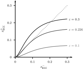
Figure 5: Density evolution for joint CAC-ECC decoding using a regular $(3,12)$ LDPC code.

Fig. 5 shows the density evolution for this setting. The threshold for the erasure channel is around $0.226$. Observe that, for an optimal code and MAP decoding, the threshold for the ECC part alone is $1-R_{\mathsf{ECC}}=0.2$. Hence, even with suboptimal codes and decoding as performed here, the joint decoding of the ECC and CAC allows us to operate above this threshold. Thus, while the minimum distance of the joint CAC-ECC scheme is the same as the minimum distance of the ECC alone by Theorem 3, joint CAC-ECC decoding nonetheless increases the decoding threshold thanks to the valuable extrinsic information provided by the CAC.

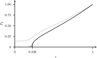
(a) Probability of bit error $P_{b}$.

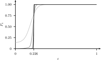
(b) Probability of block error $P_{e}$.

Figure 6: Monte-Carlo simulations of the probabilities of bit and block error for a regular $(3,12)$ LDPC code. The plots are for block lengths of $N\in\{10^{2},10^{3},10^{4},10^{5}\}$ (from light gray to black). A phase transition at the analytically derived threshold of $0.226$ is apparent.

We complement the asymptotic analysis with simulation results for a joint CAC+ECC encoder and decoder. In our simulation setting, we use a fixed block length of $N$ and generate the past bus state $\bm{a}$ uniformly at random over $\{0,1\}^{N}$. Since we are interested in the asymptotic behavior, we do not handle the case with insufficient free wires and simply declare an error in this case. Fig. 6 shows the resulting probabilities of bit and block error for a regular $(3,12)$ LDPC code for $N\in\{10^{2},10^{3},10^{4},10^{5}\}$. Both error probabilities exhibit a clear phase transition at the theoretically derived threshold of $0.226$ as expected. These simulation results also validate the modified ensemble (with variable length of the prior bus state $\bm{a}$) used for the asymptotic analysis.

It is worth commenting on the behavior of the curves around erasure rate $\varepsilon=0$. The error probability is not zero in this regime due to insufficient free wires being treated as error events. For $N=10^{2}$ and $R_{\mathsf{ECC}}=0.8$ as used here, a Binomial approximation estimates this error event as happening with probability $0.149$. The simulation results for $N=10^{2}$ yield $P_{e}(0)\approx 0.141$. As the block length increases, this error event has exponentially decreasing probability and is no longer apparent on the plots. ∎

Appendix A Proof of Theorem 1

Figure 7: Shielded joint CAC-ECC encoder from [10].

The shielded joint CAC-ECC encoder from [10] has the structure shown in Fig. 7. By definition,

$$R_{\mathsf{S}} =\frac{K}{L+M},$$

$$R_{\mathsf{CAC}} =\frac{K}{L},$$

$$R_{\mathsf{ECC}} =\frac{L}{L+P}.$$

Since the parity bits are duplicated we have,

$$\frac{P}{M} =\frac{1}{2}.$$

From the equation for $R_{\mathsf{ECC}}$ we can solve for $P/L$ as

$$\frac{P}{L}=R_{\mathsf{ECC}}^{-1}-1.$$

Now,

$$R_{\mathsf{S}}^{-1} =\frac{L}{K}+\frac{M}{K}$$

$$=\frac{L}{K}+\frac{L}{K}\cdot\frac{P}{L}\cdot\frac{M}{P}$$

$$=R_{\mathsf{CAC}}^{-1}+R_{\mathsf{CAC}}^{-1}\cdot\bigl{(}R_{\mathsf{ECC}}^{-1}-1\bigr{)}\cdot 2$$

$$=R_{\mathsf{CAC}}^{-1}\bigl{(}2R_{\mathsf{ECC}}^{-1}-1\bigr{)},$$

so that

$$R_{\mathsf{S}}=R_{\mathsf{CAC}}\bigl{(}2R_{\mathsf{ECC}}^{-1}-1\bigr{)}^{-1}$$

as claimed. ∎

Appendix B Proof of Theorem 2

Since we send $K$ information bits over the $N$-wire bus, the rate of the joint CAC and ECC scheme is given by $R_{\mathsf{E}}=K/N$. We want to express this in terms of the rate of the CAC and the ECC. Since $N-P$ bits on the non-free wires are used to generate the $P$ parity bits, and since we assume that $\bm{a}$ has a sufficient number of free wires to carry those parities, we have

$$R_{\mathsf{ECC}} =\frac{N-P}{N}.$$

We next compute the rate of the CAC encoder. Recall that this rate depends on the past state $\bm{a}$. Since the past bus state gives rise to $P$ free wires, the CAC encoder can put any information on these $P$ wires without affecting the setting of bits on the non-free wires. Thus, we have $K+P$ information bits encoded by the CAC to $N$ bits (refer to Fig. 2 in Section III). Thus, we have

$$R_{\mathsf{CAC}} =\frac{K+P}{N}.$$

From the equation for $R_{\mathsf{ECC}}$ we can solve for $P/N$ as

$$\frac{P}{N}=1-R_{\mathsf{ECC}}.$$

Hence,

$$R_{\mathsf{E}} =\frac{K}{N}$$

$$=\frac{K+P}{N}-\frac{P}{N}$$

$$=R_{\mathsf{CAC}}+R_{\mathsf{ECC}}-1,$$

as required. ∎

Appendix C Proof that $R_{\mathsf{E}}\geq R_{\mathsf{S}}$

We now show that $R_{\mathsf{E}}(\bm{a})\geq R_{\mathsf{S}}(\bm{a})$ for all possible past bus states $\bm{a}$ with sufficient number of free wires.

We start by lower bounding $R_{\mathsf{CAC}}(\bm{a})$. Recall that there are $P$ free wires on the bus, each of which can carry one information bit. Furthermore, using the shielding argument seen earlier, we can transmit at least $d/2$ bits for each alternating run in $\bm{a}$ of any length $d$. This implies that the number of information bits that the single CAC can send is at least

$$P+(N-P)/2=(N+P)/2.$$

Hence,

$$R_{\mathsf{CAC}}(\bm{a})\geq(1+P/N)/2.$$

Since $P/N=1-R_{\mathsf{ECC}}$, this implies

$$R_{\mathsf{CAC}}(\bm{a})\geq(1+1-R_{\mathsf{ECC}})/2=1-R_{\mathsf{ECC}}/2.$$ (4)

From this, we obtain that

$$R_{\mathsf{E}}(\bm{a})-R_{\mathsf{S}}(\bm{a}) =R_{\mathsf{CAC}}(\bm{a})+R_{\mathsf{ECC}}-1-\frac{R_{\mathsf{CAC}}(\bm{a})R_{\mathsf{ECC}}}{2-R_{\mathsf{ECC}}}$$

$$=R_{\mathsf{CAC}}(\bm{a})\frac{1-R_{\mathsf{ECC}}}{1-R_{\mathsf{ECC}}/2}+R_{\mathsf{ECC}}-1$$

$$\stackrel{{\scriptstyle\eqref{eq:boundRcac}}}{{\geq}}0.$$

∎

Appendix D Proof of Theorem 3

Denote by $\mathcal{C}_{\mathsf{ECC}}$ and $\mathcal{C}_{\mathsf{CAC}}$ the collection of all codewords of the ECC and CAC, respectively. We have dropped the dependence of the CAC on the past bus state $\bm{a}$ from the notation, but we stress that $\mathcal{C}_{\mathsf{CAC}}$ depends on $\bm{a}$. Recall the notation $d_{\mathsf{E}}=d_{\mathsf{E}}(\bm{a})$ for the minimum distance of the embedded joint CAC and ECC scheme. Since every codeword of the joint CAC-ECC is in particular an element of $\mathcal{C}_{\mathsf{ECC}}$, we clearly have $d_{\mathsf{E}}\geq d_{\mathsf{ECC}}$. We next prove the reverse inequality. In the following we use the notation $[N]$ to denote the set $\{1,2,3,\dots,N\}$.

Let $\mathcal{P}\subset[N]$ be the location of the parity bits and set $\mathcal{I}\mathrel{\triangleq}[N]\setminus\mathcal{P}$. For a vector $\bm{c}$ of length $N$, define $\bm{c}(\mathcal{I})\mathrel{\triangleq}(c_{n})_{n\in\mathcal{I}}$, and similarly define $\mathcal{C}_{\mathsf{CAC}}(\mathcal{I})$. Note that, since $\mathcal{P}$ are the free wires with respect to $\bm{a}$, we can decide if a vector $\bm{c}$ is in $\mathcal{C}_{\mathsf{CAC}}$ by only considering $\bm{c}(\mathcal{I})$. With slight abuse of notation, we can therefore write $\bm{c}(\mathcal{I})\in\mathcal{C}_{\mathsf{CAC}}(\mathcal{I})$ to mean that $\bm{c}\in\mathcal{C}_{\mathsf{CAC}}$.

Let $\bm{c}^{(0)}\in\mathcal{C}_{\mathsf{ECC}}$ be a nonzero codeword of minimum weight, i.e., $d_{\mathsf{ECC}}$ by linearity of the ECC. Note that $\bm{c}^{(0)}$ might not be an element of $\mathcal{C}_{\mathsf{CAC}}$. However, we next prove that we can find $\bm{c}^{(1)}(\mathcal{I})\in\mathcal{C}_{\mathsf{CAC}}(\mathcal{I})$ such that

$$\bm{c}^{(2)}(\mathcal{I})\mathrel{\triangleq}\bm{c}^{(0)}(\mathcal{I})\oplus\bm{c}^{(1)}(\mathcal{I})\in\mathcal{C}_{\mathsf{CAC}}(\mathcal{I}).$$ (5)

If this is the case, then we can find the whole codewords $\bm{c}^{(1)}$ and $\bm{c}^{(2)}$ in $\mathcal{C}_{\mathsf{ECC}}$ by computing the necessary parities of $\bm{c}^{(1)}(\mathcal{I})$ and $\bm{c}^{(2)}(\mathcal{I})$ (recall that the ECC is systematic with the parity bits at locations $\mathcal{P}=[N]\setminus\mathcal{I}$). By construction, we then have $\bm{c}^{(1)},\bm{c}^{(2)}\in\mathcal{C}_{\mathsf{ECC}}\cap\mathcal{C}_{\mathsf{CAC}}$. Moreover, by linearity of the ECC, $\bm{c}^{(2)}=\bm{c}^{(0)}\oplus\bm{c}^{(1)}$. Hence, the distance between $\bm{c}^{(1)}$ and $\bm{c}^{(2)}$ is $\bm{c}^{(1)}\oplus\bm{c}^{(2)}=\bm{c}^{(0)}$, which shows that $d_{\mathsf{E}}\leq d_{\mathsf{ECC}}$, as required.

It remains to construct $\bm{c}^{(1)}(\mathcal{I})\in\mathcal{C}_{\mathsf{CAC}}(\mathcal{I})$ such that (5) holds. Parse the past bus state $\bm{a}$ into alternating runs, where each such run is a contiguous subsequence of the form $0101\dots$ or $1010\dots$. Recall from Section II that the CAC constraints are active only within each such run, but not across its boundaries. Consequently, we can construct $\bm{c}^{(1)}(\mathcal{I})$ for each such run independently and then simply concatenate the resulting pieces. In the following, we will therefore consider, without loss of generality, a past bus state $\bm{a}$ whose restriction $\bm{a}(\mathcal{I})$ consists of a single alternating run, say $0101\dots$.

We explain the procedure of constructing $\bm{c}^{(1)}(\mathcal{I})\in\mathcal{C}_{\mathsf{CAC}}(\mathcal{I})$ with the help of an example summarized in the following table where each row corresponds to a vector of $|\mathcal{I}|=11$ bits.

$$\begin{array}[]{c|ccccccccccc}\bm{a}(\mathcal{I})&0&1&0&1&0&1&0&1&0&1&0\\ \bm{c}^{(0)}(\mathcal{I})&1&1&0&{\color[rgb]{1,0,0}\bm{0}}&{\color[rgb]{1,0,0}\bm{1}}&{\color[rgb]{1,0,0}\bm{0}}&{\color[rgb]{1,0,0}\bm{1}}&1&{\color[rgb]{1,0,0}\bm{1}}&{\color[rgb]{1,0,0}\bm{0}}&0\\ \bm{c}^{(1)}(\mathcal{I})&0&0&0&{\color[rgb]{1,0,0}\bm{1}}&{\color[rgb]{1,0,0}\bm{1}}&{\color[rgb]{1,0,0}\bm{1}}&{\color[rgb]{1,0,0}\bm{0}}&0&{\color[rgb]{1,0,0}\bm{0}}&{\color[rgb]{1,0,0}\bm{1}}&0\\ \bm{c}^{(2)}(\mathcal{I})&1&1&0&1&0&1&1&1&1&1&0\end{array}$$

Observe that we can parse $\bm{c}^{(0)}(\mathcal{I})$ into positions where the CAC constraints are satisfied with respect to $\bm{a}(\mathcal{I})$ and alternating runs where the constraints are violated (indicated in bold red in the table). At positions where $\bm{c}^{(0)}(\mathcal{I})$ satisfies the CAC constraints, we set $\bm{c}^{(1)}(\mathcal{I})$ to $0$. Consider then a run of violated constraints in $\bm{c}^{(0)}(\mathcal{I})$. Notice that each such run has length at least $2$. If required, we choose the first and last bit in this run in $\bm{c}^{(1)}(\mathcal{I})$ such that the CAC constraints are satisfied. The remaining bits in this run in $\bm{c}^{(1)}(\mathcal{I})$ are set to $1$. With this construction, there is at least one value of $1$ in every alternating position of the run of violated CAC constraints. This is enough to ensure that $\bm{c}^{(2)}(\mathcal{I})=\bm{c}^{(0)}(\mathcal{I})\oplus\bm{c}^{(1)}(\mathcal{I})$ satisfies the CAC constraints, as needed to be shown. ∎

Appendix E Proof of Theorem 4

Throughout this section, we make the assumption that the local decoding neighborhood of each node is a tree. This assumption holds with high probability asymptotically as $N\to\infty$.

The density evolution for the ECC part of the factor graph is standard. A message from an information variable node to a ECC-check node is an erasure if and only if the variable node is erased by the channel, the message from the CAC-check node is an erasure, and the messages from all ECC-check nodes over the edges other then the current one are erasures. Thus, the probability of erasure is

$$x_{\mathsf{ECC}}=\varepsilon y_{\mathsf{CAC}}\lambda(y_{\mathsf{ECC}}).$$

A message from an ECC check node to an information variable node is an erasure unless all other incoming edges carry non-erasures. The probability of erasure is

$$y_{\mathsf{ECC}}=1-(1-x_{\mathsf{P}})^{2}\rho(1-x_{\mathsf{ECC}}).$$

Here, the factor $(1-x_{\mathsf{P}})^{2}$ arises because each ECC-check is also connected to two additional parity bits from $\bm{a}_{2}$ (refer to Fig. 4).

A message from a parity variable node to an ECC-check node is an erasure if the channel and the other edge coming from the ECC-check are erasures so that

$$x_{\mathsf{P}}=\varepsilon y_{\mathsf{P}}.$$

A message from an ECC-check node to a parity variable node is an erasure unless all its incoming messages are non-erasures so that

$$y_{\mathsf{P}}=1-(1-x_{\mathsf{P}})R(1-x_{\mathsf{ECC}}).$$

Consider next a message from an information variable node to a CAC-check node. This message is an erasure if and only if the variable node is erased by the channel and the messages from all ECC-check nodes are erasures. Hence, the probability of erasure is

$$x_{\mathsf{CAC}}=\varepsilon L(y_{\mathsf{ECC}}).$$

Consider finally a message from a CAC-check node to an information variable node. Recall that the probability that this edge is connected to a CAC-check node of degree $d$ is $\tilde{\rho}_{d}$. Let $Y$ be the random variable describing the message over the edge under consideration, and let $D$ be the random variable describing the degree of the CAC-check node under consideration. Then the probability of erasure is

$$y_{\mathsf{CAC}}=\sum_{d=1}^{\infty}\tilde{\rho}_{d}\mathbb{P}(Y=\,?\mid D=d)=1-\sum_{d=1}^{\infty}\tilde{\rho}_{d}\mathbb{P}(Y\neq\,?\mid D=d).$$ (6)

If $d=1$, then the message from this CAC-check node is an erasure with probability one, so that

$$\mathbb{P}(Y\neq{?}\mid D=1)=0.$$ (7)

Consider next $d=2$ and assume that the edge under consideration is the first one. There are two equally likely possible alternating runs in $\bm{a}$ that can correspond to this CAC check node, $01$ and $10$. Assume for the moment that the run is $01$. The set of all possible two-bit sequences in $\bm{b}$ satisfying the CAC constraint is then $\{00,01,11\}$. By construction, these three possible sequences occur with uniform probability in the code ensemble. Note that $Y$ is a non-erasure if and only if the corresponding variable node has a value that is forced by its neighboring variable node. Here, this happens if the neighboring (second) variable node takes value $0$ and is not erased, which forces the first variable node to have value $0$ as well. This situation holds in one of the three possible sequences above, and the probability of non-erasure is $1-x_{\mathsf{CAC}}$. By symmetry, the same reasoning is valid if the edge under consideration is the second one. Finally, again by symmetry, the same conclusion holds if the alternating run in $\bm{a}$ is $10$. Thus,

$$\mathbb{P}(Y\neq{?}\mid D=2) =\frac{1}{3}(1-x_{\mathsf{CAC}})$$

$$=\frac{1}{2}\cdot 2\frac{F(1)}{F(4)}(1-x_{\mathsf{CAC}})$$

$$=\frac{1}{2}\sum_{i=1}^{2}p_{2,i}(x_{\mathsf{CAC}}).$$

Consider then $d=3$. There are again two equally likely possible past bus states, $010$ and $101$. Assume for now that we are in the first case. The set of all possible three-bit sequences in $\bm{b}$ satisfying the CAC constraints are $\{000,010,011,110,111\}$, and each of them has probability $1/5=1/F(5)$ by construction.

Assume that the edge under consideration is the first one (i.e., $i=1$). For the first variable node to be forced, the second variable node has to take value $0$. This happens for one out of the five possible sequences, namely $000$. Thus, for $i=1$, the probability of $Y$ being a non-erasure is

$$\frac{1}{5}\cdot(1-x_{\mathsf{CAC}})=\frac{F(2)}{F(5)}\cdot(1-x_{\mathsf{CAC}})=p_{3,1}(x_{\mathsf{CAC}}).$$

By an analogous argument, for $i=3$, the probability of $Y$ being a non-erasure is

$$\frac{1}{5}\cdot(1-x_{\mathsf{CAC}})=\frac{F(2)}{F(5)}\cdot(1-x_{\mathsf{CAC}})=p_{3,3}(x_{\mathsf{CAC}}).$$

For the middle edge ($i=2$), the variable node is forced if either neighboring variable node takes value $1$. There is one sequence $111$ for which both these neighboring variable nodes have to be erased in order for the current message to be an erasure. There are two messages $\{011,110\}$ for which only one neighboring variable node has to be erased in order for the current message to be an erasure. Thus, for $i=2$, the probability of $Y$ being a non-erasure is

$$\frac{2}{5}\cdot(1-x_{\mathsf{CAC}})+\frac{1}{5}\cdot(1-x_{\mathsf{CAC}}^{2})=\frac{F(1)F(2)+F(2)F(1)}{F(5)}\cdot(1-x_{\mathsf{CAC}})+\frac{F(1)F(1)}{F(5)}\cdot(1-x_{\mathsf{CAC}}^{2})=p_{3,2}(x_{\mathsf{CAC}}).$$

This argument was for alternating run in $\bm{a}$ of $010$. By symmetry, the same conclusion holds if the alternating run in $\bm{a}$ is $101$. Since the edge is in relative position $i$ with probability $1/3$, we thus have

$$\mathbb{P}(Y\neq{?}\mid D=3)=\frac{1}{3}\sum_{i=1}^{3}p_{3,i}(x_{\mathsf{CAC}}).$$

Consider finally the case of general $d>3$. Consider first edge position $i=1$, and without loss of generality consider an alternating run in $\bm{a}$ of $0101\dots$. There are $F(d+2)$ possible sequences that satisfy the CAC constraints with respect to this alternating run. In order for the first variable to be forced to take value $0$, the sequence must be of the form $000\star\dots$, where $\star$ indicates that the corresponding value can be either $0$ or $1$. Note that the third value is forced to $0$ to satisfy the CAC constraints. There are $F(d-1)$ such sequences. Hence, for $i=1$, the probability of $Y$ being a non-erasure is

$$\frac{F(d-1)}{F(d+2)}\cdot(1-x_{\mathsf{CAC}})=p_{d,1}(x_{\mathsf{CAC}}).$$

By an analogous argument, for $i=d$, the probability of $Y$ being a non-erasure is

$$\frac{F(d-1)}{F(d+2)}\cdot(1-x_{\mathsf{CAC}})=p_{d,d}(x_{\mathsf{CAC}}).$$

Consider then $i\in\{2,3,\dots,d-1\}$, and without loss of generality consider an alternating run in $\bm{a}$ of $\dots 101{\color[rgb]{1,0,0}\bm{0}}101\dots$, where $i$ is the position indicated in bold red font. For the variable node $i$ to be constrained from both sides, the sequence in $\bm{b}$ has to be of the form $\dots\star 00{\color[rgb]{1,0,0}\bm{0}}00\star\dots$. There are $F(i-1)F(d-i)$ such sequences. For the variable node $i$ to constrained from only the left, in $\bm{b}$ has to be of the form $\dots\star 00{\color[rgb]{1,0,0}\bm{0}}1\star\star\dots$. There are $F(i-1)F(d-i+1)$ such sequences. For the variable node $i$ to be constrained from only the right, the sequence in $\bm{b}$ has to be of the form $\dots\star\star 1{\color[rgb]{1,0,0}\bm{0}}00\star\dots$. There are $F(i)F(d-i)$ such sequences. Hence, for $i\in\{2,3,\dots,d-1\}$, the probability of $Y$ being a non-erasure is

$$\frac{F(i-1)F(d-i+1)+F(i)F(d-i)}{F(d+2)}\cdot(1-x_{\mathsf{CAC}})+\frac{F(i-1)F(d-i)}{F(d+2)}\cdot(1-x_{\mathsf{CAC}}^{2})=p_{d,i}(x_{\mathsf{CAC}}).$$

These probabilities do not depend on the actual realization of the alternating run in $\bm{a}$ other than its length. Since the edge is in relative position $i$ with probability $1/d$, we thus have

$$\mathbb{P}(Y\neq{?}\mid D=d)=\frac{1}{d}\sum_{i=1}^{d}p_{d,i}(x_{\mathsf{CAC}}).$$

Substituting this expression and (7) into (6) yields that

$$y_{\mathsf{CAC}}=1-\sum_{d=2}^{\infty}\frac{\tilde{\rho}_{d}}{d}\sum_{i=1}^{d}p_{d,i}(x_{\mathsf{CAC}}).$$

This concludes the proof. ∎

References

- [1] G. D. Micheli and L. Benini, “Networks on chips: a new SoC paradigm,” Computer, vol. 35, pp. 70–78, Jan. 2002.
- [2] G. D. Micheli, C. Seiculescu, S. Murali, L. Benini, F. Angiolini, and A. Pullini, “Networks on chips: From research to products,” in Proc. ACM/IEEE DAC, pp. 300–305, June 2010.
- [3] N. R. Shanbhag, “Reliable and efficient system-on-chip design,” Computer, vol. 37, pp. 42–50, Mar. 2004.
- [4] R. Ho, K. W. Mai, and M. A. Horowitz, “The future of wires,” Proc. IEEE, vol. 89, pp. 490–504, Apr. 2001.
- [5] P. P. Sotiriadis, Interconnect modeling and optimization in deep submicron technologies. PhD thesis, MIT, 2002.
- [6] B. Victor and K. Kreutzer, “Bus encoding to prevent crosstalk delay,” Proc. IEEE/ACM ICCAD, pp. 57–63, Nov. 2001.
- [7] T. K. Konstantakopoulos, “Implementation of delay and power reduction in deep sub-micron buses using coding,” Master’s thesis, MIT, 2002.
- [8] C.-S. Changa, J. Cheng, T.-K. Huang, X.-C. Huang, and D.-S. Lee, “A bit-stuffing algorithm for crosstalk avoidance in high speed switching,” in Proc. IEEE INFOCOMM, pp. 1–9, Mar. 2010.
- [9] “DDR4 SDRAM standard.” JEDEC, 2013.
- [10] S. R. Sridhara and N. R. Shanbhag, “Coding for system-on-chip networks: A unified framework,” IEEE Trans. VLSI Syst., vol. 13, pp. 655–667, June 2005.
- [11] S. R. Sridhara and N. R. Shanbhag, “Coding for reliable on-chip buses: A class of fundamental bounds and practical codes,” IEEE Trans. Comput.-Aided Design Integr. Circuits Syst., vol. 26, pp. 977–982, May 2007.
- [12] H. Jin, A. Khandekar, and R. McEliece, “Irregular repeat-accumulate codes,” Proc. 2nd Int. Symp. Turbo Codes, pp. 1–8, Sept. 2000.
- [13] T. Richardson and R. Urbanke, Modern Coding Theory. Cambridge University Press, 2008.
- [14] H.-A. Loeliger, “An introduction to factor graphs,” IEEE Signal Process. Mag., vol. 21, pp. 28–41, Jan. 2004.
- [15] P. P. Sotiriadis and A. Chandrakasan, “A bus energy model for deep submicron technology,” IEEE Trans. VLSI Syst., vol. 10, pp. 341–350, June 2002.
- [16] P. P. Sotiriadis and A. Chandrakasan, “Reducing bus delay in submicron technology using coding,” in Proc. IEEE ASP-DAC, pp. 109–114, Feb. 2001.
- [17] T. Richardson and R. Urbanke, “The capacity of low-density parity check codes under message-passing decoding,” IEEE Trans. Inform. Theory, vol. 47, pp. 599–618, Feb. 2001.
- [18] T. Richardson, A. Shokrollahi, and R. Urbanke, “Design of capacity-approaching irregular low-density parity-check codes,” IEEE Trans. Inform. Theory, vol. 47, pp. 619–637, Feb. 2001.