Uniformly accurate time-splitting methods for the semiclassical linear Schrödinger equation

Abstract.

This article is devoted to the construction of numerical methods which remain insensitive to the smallness of the semiclassical parameter for the linear Schrödinger equation in the semiclassical limit. We specifically analyse the convergence behavior of the first-order splitting. Our main result is a proof of uniform accuracy. We illustrate the properties of our methods with simulations.

1. Introduction

We are concerned here with the uniformly accurate numerical approximation of the solution ${\Psi^{\varepsilon}}:{\mathbb{R}}_{+}\times{\mathbb{R}}^{d}\to{\mathbb{C}}$, $d\geq 1$, of the linear Schrödinger equation in its semiclassical limit

$$i\varepsilon\partial_{t}{\Psi^{\varepsilon}}=-\frac{\varepsilon^{2}}{2}\Delta{\Psi^{\varepsilon}}+\mathcal{V}{\Psi^{\varepsilon}}$$ (1.1)

where $\mathcal{V}$ is a smooth potential which does not depend on time. The initial datum is assumed to be of the form

$${\Psi^{\varepsilon}}(0,\cdot)=A_{0}(\cdot)e^{iS_{0}(\cdot)/\varepsilon}\quad\mbox{ with }\quad\|A_{0}\|_{L^{2}({\mathbb{R}}^{d})}=1.$$ (1.2)

Note that the $L^{2}$-norm, the energy and the momentum of ${\Psi^{\varepsilon}}(0,\cdot)$, namely

Mass: $$\|{\Psi^{\varepsilon}}(t,\cdot)\|_{L^{2}({\mathbb{R}}^{d})}^{2},$$ (1.3)

Energy: $$\int_{{\mathbb{R}}^{d}}\left(\varepsilon^{2}|\nabla{\Psi^{\varepsilon}}(t,x)|^{2}+\mathcal{V}|{\Psi^{\varepsilon}}(t,x)|^{2}\right)dx,$$ (1.4)

Momentum: $$\varepsilon\operatorname{Im}\int_{{\mathbb{R}}^{d}}\overline{{\Psi^{\varepsilon}}(t,x)}\nabla{\Psi^{\varepsilon}}(t,x)dx,$$ (1.5)

are all preserved by the flow of (1.1), whenever ${\Psi^{\varepsilon}}(0,\cdot)\in H^{1}({\mathbb{R}}^{d})$.

Owing to its numerous occurrences in a vast number of domains of applications in physics, equation (1.1) has been widely studied (see for instance [27, 32] and the references therein). In the semiclassical regime where the rescaled Planck constant $\varepsilon$ is small, its asymptotic study allows for an appropriate description of the observables of ${\Psi^{\varepsilon}}$ through the laws of hydrodynamics. We refer to [12] for a detailed presentation of the semiclassical analysis and to [25] for a review of both theoretical and numerical issues.

Let us also mention that we do not consider the case where the initial datas are Gaussian wave packets for which efficient schemes have already been developed [22, 21, 23].

1.1. Motivation

Generally speaking, numerical methods for equation (1.1) exhibit an error of size $\Delta t^{p}/\varepsilon^{r}+\Delta x^{q}/\varepsilon^{s}$, where $\Delta t$ and $\Delta x$ are the time and space steps and $p,q,r,s$ strictly positive numbers. For time-splitting methods for instance, the error on the wave function behaves like $\Delta x/\varepsilon+\Delta t^{p}/\varepsilon$ [5, 17]. Even if we content ourselves with observables, the error of a splitting method of Bao, Jin, and Markowich [5] grows like $\Delta x/\varepsilon+\Delta t^{p}$. Now, achieving a fixed accuracy for varying values of $\varepsilon$ requires to keep both ratios $\Delta t/\varepsilon^{r/p}$ and $\Delta x/\varepsilon^{s/q}$ constant, and becomes prohibitively costly when $\varepsilon\to 0$. Our aim, in this article, is thus to develop new numerical schemes that are Uniformly Accurate (UA) w.r.t. $\varepsilon$, i.e. whose accuracy does not deteriorate for vanishing $\varepsilon$. In other words, schemes for which $r,s=0$. This seems highly desirable as all available methods with the exception of [9], namely finite difference methods [1, 16, 26, 35], splitting methods [8, 17, 18, 29, 31, 34], asymptotic splitting methods [3, 4], relaxation schemes [7] and symplectic methods [33] fail to be UA.

It is the belief of the authors that, prior to the construction of UA-schemes, it is necessary to reformulate (1.1) as in [9] and we now describe how this can be done.

1.2. Reformulation of the problem

In the spirit of the Wentzel-Kramers-Brillouin (WKB) techniques, we decompose ${\Psi^{\varepsilon}}$ as the product of a slowly varying amplitude and a fast oscillating factor

$${\Psi^{\varepsilon}}(t,\cdot)={A^{\varepsilon}}(t,\cdot)e^{i{S^{\varepsilon}}(t,\cdot)/\varepsilon}.$$ (1.7)

From this point onwards, various choices are possible, depending on whether ${A^{\varepsilon}}$ is complex or not: taking ${A^{\varepsilon}}\in{\mathbb{C}}$ leads to the following system [12]

$$\partial_{t}{S^{\varepsilon}}+\frac{|\nabla{S^{\varepsilon}}|^{2}}{2}+\mathcal{V}=0,$$ (1.8a)

$$\partial_{t}{A^{\varepsilon}}+\nabla{S^{\varepsilon}}\cdot\nabla{A^{\varepsilon}}+\frac{{A^{\varepsilon}}}{2}\Delta{S^{\varepsilon}}=\frac{i\varepsilon\Delta{A^{\varepsilon}}}{2}$$ (1.8b)

with ${S^{\varepsilon}}(0,\cdot)=S_{0}(\cdot)$ and ${A^{\varepsilon}}(0,\cdot)=A_{0}(\cdot)$. Under appropriate smoothness assumptions, $({A^{\varepsilon}},{S^{\varepsilon}})\in{\mathbb{C}}\times{\mathbb{R}}$ converges when $\varepsilon\to 0$ to the solution $({A^{0}},{S^{0}})$ of

$$\partial_{t}{S^{0}}+\frac{|\nabla{S^{0}}|^{2}}{2}+\mathcal{V}=0,$$ (1.9a)

$$\partial_{t}{A^{0}}+\nabla{S^{0}}\cdot\nabla{A^{0}}+\frac{{A^{0}}}{2}\Delta{S^{0}}=0.$$ (1.9b)

Notice that $(\rho,v)=(|{A^{0}}|^{2},\nabla{S^{0}})$ is then solution of the Euler system

$$\partial_{t}v+v\cdot\nabla v+\nabla\mathcal{V}=0,$$ (1.10a)

$$\partial_{t}\rho+\operatorname{div}(\rho v)=0.$$ (1.10b)

Now, an important drawback of (1.8) stems from the formation of caustics in finite time [12]: the solution of (1.8) may indeed cease to be smooth even though ${\Psi^{\varepsilon}}$ is globally well-defined for $\varepsilon>0$. In order to obtain global existence for $\varepsilon>0$, Besse, Carles and Méhats [9] suggested an alternative formulation by introducing an asymptotically-vanishing viscosity term in the eikonal equation (1.8a). Therein, system (1.8) is replaced by

$$\partial_{t}{S^{\varepsilon}}+\frac{|\nabla{S^{\varepsilon}}|^{2}}{2}+\mathcal{V}=\varepsilon^{2}\Delta{S^{\varepsilon}},$$ (1.11a)

$$\partial_{t}{A^{\varepsilon}}+\nabla{S^{\varepsilon}}\cdot\nabla{A^{\varepsilon}}+\frac{{A^{\varepsilon}}}{2}\Delta{S^{\varepsilon}}=\frac{i\varepsilon\Delta{A^{\varepsilon}}}{2}-i\varepsilon{A^{\varepsilon}}\Delta{S^{\varepsilon}}$$ (1.11b)

where ${S^{\varepsilon}}(0,x)=S_{0}(x)$, ${A^{\varepsilon}}(0,x)=A_{0}(x)$ and where $x\in{\mathbb{R}}^{d}$. Let us emphasize that both (1.8) and (1.11) are equivalent to (1.1) in the following sense: as long as the solution $({S^{\varepsilon}},{A^{\varepsilon}})$ of (1.8) (resp. (1.11)) is smooth, the function ${\Psi^{\varepsilon}}$ defined by (1.7) solves (1.1). The well-posedeness of (1.11) and the uniform control of the solutions with respect to $\varepsilon$ are stated in Theorem 2.1 below.

The main advantage of the WKB reformulation (1.11) over (1.1) is apparent: the semiclassical parameter $\varepsilon$ does not give rise to singular perturbations. Hence, it constitutes a good basis for the development of UA schemes (at least prior to the appearance of caustics), as witnessed by the methods introduced later in this paper.

1.3. Construction of the schemes

First and only (up to our knowledge) UA schemes are based on the formulation (1.11) introduced in [9]. Nevertheless, these schemes are still subject to CFL stability conditions and are of low order in time and space. In this paper, we consider, in lieu of finite differences as in [9], time-splitting methods, for they enjoy the following favorable features:

1. they do not suffer from stability restrictions on the time step;

2. they are easy to implement;

3. they preserve exactly the $L^{2}$-norm;

4. they can be adapted to semilinear Schrödinger equations;

5. they can be composed to attain high-order of convergence in time while remaining spectrally convergent in space.

Points (iv) and (v) will be addressed in a forthcoming work using complex time steps (see [10]), while, in this paper, we introduce first and second order in time splitting-schemes and concentrate on the numerical analysis of the first-order one for the sake of clarity.

System (1.11) is split into four pieces as follows:

First flow: We denote $\varphi^{1}_{h}$ the approximate flow at time $h\in{\mathbb{R}}$ of the system

$$\partial_{t}S+\frac{|\nabla S|^{2}}{2}=0,$$ (1.13a)

$$\partial_{t}A+\nabla S\cdot\nabla A+\frac{A}{2}\Delta S=\frac{i\Delta A}{2}.$$ (1.13b)

The eikonal equation (1.13a) is solved by means of the method of characteristics, while equation (1.13b) is dealt with by noticing that $w=A\exp\left(iS\right)$ satisfies the free Schrödinger equation $i\partial_{t}w=-\frac{1}{2}\Delta w$.

Second flow: We define $\varphi^{2}_{h}$ as the exact flow at time $h\in{\mathbb{R}}$ of the system

$$\partial_{t}S=0,$$ (1.14a)

$$\partial_{t}A=\frac{i\left(\varepsilon-1\right)\Delta A}{2},$$ (1.14b)

which is solved in the Fourier space.

Third flow: The third flow $\varphi^{3}_{h}$ is defined as the exact flow at time $h\in{\mathbb{R}}$ of system

$$\partial_{t}S=-\mathcal{V},$$ (1.15a)

$$\partial_{t}A=0.$$ (1.15b)

Fourth flow: The fourth flow $\varphi^{4}_{h}$ is defined as the exact flow at time $h\in{\mathbb{R}}_{+}$ of

$$\partial_{t}S=\varepsilon^{2}\Delta S,$$ (1.16a)

$$\partial_{t}A=-i\varepsilon A\Delta S.$$ (1.16b)

Equation (1.16a) is solved in Fourier space and the solution of (1.16b) is simply obtained through the formula $A(h,\cdot)=\exp\left(-i\varepsilon^{-1}(S(h,\cdot)-S(0,\cdot))\right)A(0,\cdot)$. Notice that $\varphi^{4}_{h}$ can thus be viewed as a regularizing flow.

The first-order scheme that we consider for (1.11) is then the concatenation of all previous flows

$$\varphi^{1}_{h}\circ\varphi^{2}_{h}\circ\varphi^{3}_{h}\circ\varphi^{4}_{h}$$ (1.17)

while the second-order scheme is given by

$$\varphi^{1}_{h/2}\circ\varphi^{2}_{h/2}\circ\varphi^{3}_{h/2}\circ\varphi^{4}_{h}\circ\varphi^{3}_{h/2}\circ\varphi^{2}_{h/2}\circ\varphi^{1}_{h/2}.$$ (1.18)

1.4. Main result

The main result of this paper is the following theorem: it states that $\varphi^{1}_{h}\circ\varphi^{2}_{h}\circ\varphi^{3}_{h}\circ\varphi^{4}_{h}$ is uniformly accurate w.r.t. the semi-classical parameter $\varepsilon$. The proper statement of the result uses the norm $\|\cdot\|_{s}$ on the set $\Sigma_{s}=H^{s+2}({\mathbb{R}}^{d})\times H^{s}({\mathbb{R}}^{d})$ defined for $s\geq 0$ and $u=(S,A)$ by

$$\left\|u\right\|_{s}=\left(\|S\|_{H^{s+2}({\mathbb{R}}^{d})}^{2}+\|A\|_{H^{s}({\mathbb{R}}^{d})}^{2}\right)^{1/2}.$$

Theorem 1.1.

Let $s>d/2+1$, $\varepsilon_{max}>0$, $u_{0}\in\Sigma_{s+2}$ and $0<T<T_{max}$ where

$$T_{max}=\sup\{t>0:\tau\mapsto\phi^{0}_{\tau}(u_{0})\in L^{\infty}([0,t];\Sigma_{s+2})\}$$

and $\phi_{\tau}^{\varepsilon}$ denotes the flow at time $\tau$ of (1.11). There exists $C>0$ and $h_{0}>0$ such that the following error estimate holds true for any $\varepsilon\in(0,\varepsilon_{max}]$, any $h\in[0,h_{0}]$ and $n\in{\mathbb{N}}$ satisfying $nh\leq T$:

$$\begin{split}&\|(\varphi^{1}_{h}\circ\varphi^{2}_{h}\circ\varphi^{3}_{h}\circ\varphi^{4}_{h})^{n}(u_{0})-\phi^{\varepsilon}_{nh}(u_{0})\|_{s}\leq Ch.\end{split}$$

The constants $C$ and $h_{0}$ do not depend on $\varepsilon$.

Remark 1.2.

The constant $T_{max}$ appearing in Theorem 1.1 is well-defined and positive since $\tau\mapsto\phi^{0}_{\tau}$ exists locally in time (see Theorem 2.1).

Remark 1.3.

The numerical analysis performed for the proof of Theorem 1.1 can immediately be extended after the caustics for $T_{max}\leq T$ and $\varepsilon>0$ since the solution of (1.11) (as the one of (1.1)) are global. Nevertheless, the constants $C$ and $h_{0}$ appearing in the result will not be independent on $\varepsilon$ anymore. This point is illustrated in Section 4.

Remark 1.4.

The proof of Theorem 1.1 can be adapted to any time-splitting method of order $1$ obtained after permutation of the four flows in (1.17).

Our proof is reminiscent of two previous results related to, on the one hand, splitting schemes for equations with Burgers nonlinearity [24] and on the other hand, splitting scheme for NLS in the semiclassical limit with [13]. Nonetheless, due to the finite-time existence of both exact and approximate flows, and to the peculiarity of the Lipschitz-type stability of the exact flows (see Lemma 2.3), our proof follows a different path. In particular, we lean the approximate solutions on the exact one to ensure that they do not blow up. Besides, the application of Lady Windermere’s fan argument is somehow hidden in an induction procedure. Finally, let us mention that, in spite of the fact that we do not specifically address this case, it is our belief that this result can be extended to Schrödinger equations with time dependent potentials, to the second-order scheme, to the Schrödinger equation with a nonlinearity of Hartree-type and to the weakly nonlinear Schrödinger equation (see also [13, Remark 4.5]).

The paper is organized as follows. In Section 2, we first give a theorem of well-posedness of the Cauchy problem for (1.11). Then Theorem 1.1 is proved using four technical lemmas. Section 3 is devoted to the proof of these lemmas. We illustrate the properties of our methods in Section 4.

2. Preparatiory results and proof of Theorem 1.1

2.1. Notations

Assume that $\varepsilon\in(0,\varepsilon_{max}]$ and $s>d/2+1$. For the sake of simplicity, we keep the notation of all the flows independent of $\varepsilon$. All the constants appearing in the proof depend on $\mathcal{V}$ but not on $\varepsilon>0$. We denote

$$\begin{split}&\varphi^{ij}_{h}=\varphi^{i}_{h}\circ\varphi^{j}_{h},\;\varphi^{ijk}_{h}=\varphi^{i}_{h}\circ\varphi^{jk}_{h},\;\\ &\varphi^{1234}_{h}=\varphi^{1}_{h}\circ\varphi^{234}_{h}=\varphi^{1}_{h}\circ\varphi^{2}_{h}\circ\varphi^{3}_{h}\circ\varphi^{4}_{h},\end{split}$$

${\mathcal{N}}_{i}$ is the possibly nonlinear operator related to $\varphi^{i}_{h}$ so that

$$\partial_{h}\varphi^{i}_{h}={\mathcal{N}}_{i}\varphi^{i}_{h}.$$

The quantities $\partial_{h}\varphi_{h}(u)$ and $\partial_{2}\varphi_{h}(u)$ are the Fréchet derivatives of $\varphi$ with respect to $h$ and $u$. The commutator of the nonlinear operators ${\mathcal{N}}_{i}$ and ${\mathcal{N}}_{j}$ is given by

$$[{\mathcal{N}}_{i},{\mathcal{N}}_{j}](u)=D{\mathcal{N}}_{i}(u)\cdot{\mathcal{N}}_{j}(u)-D{\mathcal{N}}_{j}(u)\cdot{\mathcal{N}}_{i}(u).$$

2.2. Existence, uniqueness and uniform boundedness results

The following theorem study some properties of the solutions of equations (1.11).

Theorem 2.1.

Let $\varepsilon_{max}>0$, $s>d/2+1$ and $u_{0}\in\Sigma_{s+2}$. The following two points are true.

1. The quantity

   $$T_{max}=\sup\{t>0:\phi^{0}(u_{0})\in L^{\infty}([0,t];\Sigma_{s+2})\}$$ (2.1)

   is well-defined and positive.

2. Let $0<T<T_{max}$. For all $\varepsilon\in[0,\varepsilon_{max}]$, there exists a unique solution

   $$\phi^{\varepsilon}(u_{0})\in C([0,T],\Sigma_{s+2})$$

   of the systems of equations (1.11). Moreover, $\phi^{\varepsilon}(u_{0})$ is bounded in

   $$C([0,T],\Sigma_{s+2})$$

   uniformly in $\varepsilon\in[0,\varepsilon_{max}]$.

The proof of Theorem 2.1 is given in Section 3.4.

2.3. The main lemmas

In this subsection, we present the main ingredients needed in the proof of Theorem 1.1. Their proof is postponed to Section 3.

Lemma 2.2.

Let $M>0$ and $s>d/2+1$. There exist $h_{1}=h_{1}(M)>0$ such that for any $\varepsilon\in(0,\varepsilon_{max}]$ and any $u_{0}\in\Sigma_{s}$ satisfying

$$\|u_{0}\|_{{s}}\leq M,$$

we have that the solution $\phi_{t}(u_{0})$ of equation (1.11) is well-defined on $[0,h_{1}]$ and for all $t\in[0,h_{1}]$

$$\|\phi_{t}(u_{0})\|_{{s}}\leq 2M.$$

Lemma 2.3.

Let $M>0$ and $s>d/2+1$. There exist $C_{2}=C_{2}(M)>0$ such that for any $\varepsilon\in(0,\varepsilon_{max}]$, any solutions $\phi_{t}(u_{1})\in L^{\infty}([0,T],\Sigma_{s+1})$ and $\phi_{t}(u_{2})\in L^{\infty}([0,T],\Sigma_{s})$ of equation (1.11), satisfying for all $t\in[0,T]$

$$\|\phi_{t}(u_{1})\|_{{s+1}}+\|\phi_{t}(u_{2})\|_{{s}}\leq M$$

we have

$$\|\phi_{t}(u_{1})-\phi_{t}(u_{2})\|_{{s}}\leq\|u_{1}-u_{2}\|_{{s}}\exp(C_{2}t).$$

Remark 2.4.

Let us insist on the fact that in Lemma 2.3, we have to control $\phi_{t}(u_{1})$ in $\Sigma_{s+1}$ and $\phi_{t}(u_{2})$ in $\Sigma_{s}$ to get Lipschitz-type stability in $\Sigma_{s}$.

Lemma 2.5.

Let $M>0$ and $s>d/2+1$. There exist $h_{3}=h_{3}(M)>0$ and $C_{3}=C_{3}(M)>0$ such that for any $\varepsilon\in(0,\varepsilon_{max}]$, any $u_{0}\in\Sigma_{s}$ satisfying $\|u_{0}\|_{s}\leq M$ and any $0\leq t\leq h_{3}$, we have

1. $\|\varphi^{1234}_{t}(u_{0})\|_{s}\leq 8M$.

2. Furthermore, if $u_{0}\in\Sigma_{s+2}$, then

   $$\|\varphi^{1234}_{t}(u_{0})\|_{s+2}\leq\exp\left(C_{3}t\right)\left(\|u_{0}\|_{s+2}+t\|\mathcal{V}\|_{H^{s+4}}\right).$$

Lemma 2.6.

Let $M>0$ and $s>d/2+1$. There exist $h_{4}=h_{4}(M)>0$ and $K_{4}=K_{4}(M)>0$ such that for any $\varepsilon\in(0,\varepsilon_{max}]$ and any $u_{0}\in\Sigma_{s+2}$ satisfying

$$\|u_{0}\|_{s+2}\leq M,$$

we have for any $t\in[0,h_{4}]$ that

$$\|\phi_{t}(u_{0})-\varphi_{t}^{1234}(u_{0})\|_{s}\leq K_{4}t^{2}.$$

2.4. Proof of Theorem 1.1

Let us denote

$$M_{s}^{\varepsilon}(T):=\sup\{\|\phi_{t}^{\varepsilon}(u_{0})\|_{s}:\;0\leq t\leq T\}.$$ (2.2)

for $\varepsilon\geq 0$ and $T\geq 0$.

Let $s>d/2+1$, $\varepsilon\in(0,\varepsilon_{max}]$, $u_{0}\in\Sigma_{s+2}$, $n\in{\mathbb{N}}$ and $h>0$ be such that $nh\leq T<T_{max}$ (see (2.1)). By Theorem 2.1, there exist $M_{s}$, $M_{s+1}$ and $M_{s+2}$ independent of $\varepsilon\in(0,\varepsilon_{max}]$ such that for all $\varepsilon\in(0,\varepsilon_{max}]$,

$$M^{\varepsilon}_{s}\leq M_{s},\;M^{\varepsilon}_{s+1}\leq M_{s+1}\mbox{ and }M^{\varepsilon}_{s+2}\leq M_{s+2}$$

(see (2.2)). We denote

$$\begin{split}&C=C_{3}(2M_{s}),\\ &c_{0}=\|u_{0}\|_{s+2}\exp\left(CT\right)+\|\mathcal{V}\|_{H^{s+4}}e^{2TC}/C,\\ &C^{\prime}=C_{2}(M_{s+1}+4M_{s}),\\ &\widetilde{c}=K_{4}(c_{0})ae^{C^{\prime}T}/C^{\prime}.\end{split}$$

Assume that

$$0\leq h\leq\min\left(h_{3}(c_{0}),M_{s}/\widetilde{c},h_{1}(2M_{s}),h_{4}(c_{0})\right).$$ (2.3)

Here, $h_{1}$, $C_{2}$, $h_{3}$, $h_{4}$ and $K_{4}$ are defined in Lemmas 2.2, 2.3, 2.5 and 2.6.

We show by induction on $0\leq k\leq n$ that

1. $(\varphi^{1234}_{h})^{k}(u_{0})$ is well-defined, belongs to $\Sigma_{s+2}$ and

   $$\|(\varphi^{1234}_{h})^{k}(u_{0})\|_{s+2}\leq\|u_{0}\|_{s+2}\exp\left(Ckh\right)+h\|\mathcal{V}\|_{H^{s+4}}\frac{e^{(k+1)hC}-e^{hC}}{e^{hC}-1}\leq c_{0},$$

2. $\|\phi_{kh}(u_{0})-(\varphi^{1234}_{h})^{k}(u_{0})\|_{s}\leq h^{2}K_{4}(c_{0})\frac{e^{C^{\prime}hk}-1}{e^{C^{\prime}h}-1}\leq\widetilde{c}h$,

and Theorem 1.1 follows then from point (ii) with $k=n$.

The induction hypothesis is true for $k=0$. Let us assume points (i) and (ii) true for $0\leq k\leq n-1$.

Lemma 2.5, point (i) and (2.3) ensure that

$$(\varphi^{1234}_{h})^{k+1}(u_{0})$$

is well-defined and belongs to $\Sigma_{s+2}$. By Point (ii) and (2.3), we have

$$\|(\varphi^{1234}_{h})^{k}(u_{0})\|_{s}\leq M_{s}+\|\phi_{kh}(u_{0})-(\varphi^{1234}_{h})^{k}(u_{0})\|_{s}\leq 2M_{s}.$$

By Lemma 2.5 and (2.3), we have

$$\|(\varphi^{1234}_{h})^{k+1}\|_{s+2}\leq\exp\left(Ch\right)\left(\|(\varphi^{1234}_{h})^{k}(u_{0})\|_{s+2}+h\|\mathcal{V}\|_{H^{s+4}}\right)$$

and point (i) ensures that

$$\begin{split}\|(\varphi^{1234}_{h})^{k+1}\|_{s+2}\leq\|u_{0}\|_{s+2}\exp\left(C(k+1)h\right)+h\|\mathcal{V}\|_{H^{s+4}}\frac{e^{(k+2)hC}-e^{hC}}{e^{hC}-1}\leq c_{0}.\end{split}$$

By Lemma 2.2 and (2.3), $h^{\prime}\mapsto\phi_{h^{\prime}}\circ(\varphi^{1234}_{h})^{k}(u_{0})$ is well-defined and satisfies for all $0\leq h^{\prime}\leq h$

$$\|\phi_{h^{\prime}}\circ(\varphi^{1234}_{h})^{k}(u_{0})\|_{{s}}\leq 4M_{s}.$$

By Lemma 2.3, we obtain that

$$\begin{split}&\|\phi_{h(k+1)}(u_{0})-\phi_{h}\circ(\varphi^{1234}_{h})^{k}(u_{0})\|_{{s}}\leq\|\phi_{hk}(u_{0})-(\varphi^{1234}_{h})^{k}(u_{0})\|_{s}\exp(C^{\prime}h).\end{split}$$

By Lemma 2.6, point (i) and (2.3), we get

$$\|\phi_{h}\circ(\varphi^{1234}_{h})^{k}(u_{0})-\varphi^{1234}_{h}\circ(\varphi^{1234}_{h})^{k}(u_{0})\|_{s}\leq K_{4}(c_{0})h^{2},$$

so that

$$\begin{split}&\|\phi_{h(k+1)}(u_{0})-(\varphi^{1234}_{h})^{k+1}(u_{0})\|_{{s}}\leq K_{4}(c_{0})h^{2}+\|\phi_{hk}(u_{0})-(\varphi^{1234}_{h})^{k}(u_{0})\|_{s}\exp(C^{\prime}h).\end{split}$$

By point (ii), we have then that

$$\|\phi_{h(k+1)}(u_{0})-(\varphi^{1234}_{h})^{k+1}(u_{0})\|_{{s}}\leq K_{4}(c_{0})h^{2}\left(\frac{e^{C^{\prime}h(k+1)}-1}{e^{C^{\prime}h}-1}\right).$$

Thus, points (i) and (ii) are true for $k+1$.

3. Proof of the main lemmas

3.1. Auxiliary results

Let us denote by $\left\langle\cdot,\cdot\right\rangle$ the $L^{2}$ scalar product, for $s>0$

$$\Lambda^{s}=(1-\Delta)^{s/2},$$

$$\Pi_{1}u=S,\;\Pi_{2}u=A,\mbox{ for }u=\left(\begin{array}[]{c}S\\ A\end{array}\right)$$ (3.1)

and

$$\begin{split}\left\langle u_{1},u_{2}\right\rangle_{s}&=\left\langle\Pi_{1}u_{1},\Pi_{1}u_{2}\right\rangle\\ &\quad+\left\langle\Lambda^{s+1}\nabla\Pi_{1}u_{1},\Lambda^{s+1}\nabla\Pi_{1}u_{2}\right\rangle+\operatorname{Re}\left\langle\Lambda^{s}\Pi_{2}u_{1},\Lambda^{s}\Pi_{2}u_{2}\right\rangle.\end{split}$$ (3.2)

We recall two points that will be of constant use in the following: the Sobolev space $H^{s}\subset L^{\infty}$ is an algebra for $s>d/2$ and the Kato-Ponce [28] inequality holds true:

Proposition 3.1.

Let ${s_{0}}>d/2+1$. There is $c>0$ such that for all $f\in H^{{s_{0}}}({\mathbb{R}}^{d})$ and $g\in H^{{s_{0}}-1}({\mathbb{R}}^{d})$

$$\|\Lambda^{{s_{0}}}(fg)-f\Lambda^{{s_{0}}}g\|_{L^{2}}\leq c(\|\nabla f\|_{L^{\infty}}\|g\|_{H^{{s_{0}}-1}}+\|f\|_{H^{{s_{0}}}}\|g\|_{L^{\infty}}).$$

The following lemmas will be used several times in our proof.

Lemma 3.2.

Let $s_{0}>d/2+1$. There is $C>0$ such that for all $v_{0}$, $v_{1}$ and $R\in L^{\infty}([0,h_{0}],H^{s_{0}}({\mathbb{R}}^{d})^{d})$ satisfying

$$\partial_{t}v_{0}+(v_{1}\cdot\nabla)v_{0}=R,$$

we have

$$\begin{split}\partial_{t}\|v_{0}\|_{H^{s_{0}}}^{2}&\leq C\left(\|v_{0}\|_{H^{s_{0}}}^{2}\|\nabla v_{1}\|_{L^{\infty}}+\|v_{0}\|_{H^{s_{0}}}\|v_{1}\|_{H^{s_{0}}}\|\nabla v_{0}\|_{L^{\infty}}\right)+2\left\langle\Lambda^{s_{0}}v_{0},\Lambda^{s_{0}}R\right\rangle\\ &\leq C\|v_{0}\|_{H^{s_{0}}}^{2}\|v_{1}\|_{H^{s_{0}}}+2\left\langle\Lambda^{s_{0}}v_{0},\Lambda^{s_{0}}R\right\rangle.\end{split}$$

Proof.

We have by integration by parts that

$$\begin{split}\partial_{t}\frac{\|v_{0}\|_{H^{s_{0}}}^{2}}{2}&=\left\langle\Lambda^{s_{0}}v_{0},\Lambda^{s_{0}}\partial_{t}v_{0}\right\rangle=-\left\langle\Lambda^{s_{0}}v_{0},\Lambda^{s_{0}}(v_{1}\cdot\nabla)v_{0}\right\rangle+\left\langle\Lambda^{s_{0}}v_{0},\Lambda^{s_{0}}R\right\rangle\\ &\leq\frac{1}{2}\int_{{\mathbb{R}}^{d}}|\Lambda^{s_{0}}v_{0}|^{2}\operatorname{div}v_{1}+\|v_{0}\|_{H^{s_{0}}}\|[\Lambda^{s_{0}},(v_{1}\cdot\nabla)]v_{0}\|_{L^{2}}+\left\langle\Lambda^{s_{0}}v_{0},\Lambda^{s_{0}}R\right\rangle.\end{split}$$

Proposition 3.1 ensures that

$$\begin{split}\partial_{t}\frac{\|v_{0}\|_{H^{s_{0}}}^{2}}{2}&\leq c\left(\|v_{0}\|_{H^{s_{0}}}^{2}\|\nabla v_{1}\|_{L^{\infty}}+\|v_{0}\|_{H^{s_{0}}}\|v_{1}\|_{H^{s_{0}}}\|\nabla v_{0}\|_{L^{\infty}}\right)+\left\langle\Lambda^{s_{0}}v_{0},\Lambda^{s_{0}}R\right\rangle.\end{split}$$

∎

Lemma 3.3.

Let $s_{0}>d/2+1$. There exists $C>0$ such that for all $A\in W^{1,\infty}([0,h_{0}],H^{s_{0}}({\mathbb{R}}^{d}))$, $v_{1}\in L^{\infty}([0,h_{0}],H^{s_{0}+1}({\mathbb{R}}^{d})^{d})$ and $R\in L^{\infty}([0,h_{0}],H^{s_{0}}({\mathbb{R}}^{d}))$ satisfying

$$\partial_{t}A+v_{1}\cdot\nabla A+A\frac{\operatorname{div}v_{1}}{2}=R,$$

we have,

$$\begin{split}\partial_{t}\|A\|_{H^{s_{0}}}^{2}&\leq C\left(\|A\|_{H^{s_{0}}}^{2}\|v_{1}\|_{W^{2,\infty}}+\|A\|_{H^{s_{0}}}\|v_{1}\|_{H^{s_{0}+1}}\|A\|_{W^{1,\infty}}\right)+2\operatorname{Re}\left\langle\Lambda^{s_{0}}A,\Lambda^{s_{0}}R\right\rangle\\ &\leq C\|A\|_{H^{s_{0}}}^{2}\|v_{1}\|_{H^{s_{0}+1}}+2\operatorname{Re}\left\langle\Lambda^{s_{0}}A,\Lambda^{s_{0}}R\right\rangle.\end{split}$$

Proof.

We have by integration by parts that

$$\begin{split}\partial_{t}\frac{\|A\|_{H^{s_{0}}}^{2}}{2}&=\operatorname{Re}\left\langle\Lambda^{s_{0}}A,\Lambda^{s_{0}}\partial_{t}A\right\rangle=-\operatorname{Re}\left\langle\Lambda^{s_{0}}A,\left(v_{1}\cdot\nabla+\frac{\operatorname{div}v_{1}}{2}\right)\Lambda^{s_{0}}A\right\rangle\\ &\quad-\operatorname{Re}\left\langle\Lambda^{s_{0}}A,\left[\Lambda^{s_{0}},\left(v_{1}\cdot\nabla+\frac{\operatorname{div}v_{1}}{2}\right)\right]A\right\rangle+\operatorname{Re}\left\langle\Lambda^{s_{0}}A,\Lambda^{s_{0}}R\right\rangle\\ &\leq\|A\|_{H^{s_{0}}}\left\|\left[\Lambda^{s_{0}},\left(v_{1}\cdot\nabla+\frac{\operatorname{div}v_{1}}{2}\right)\right]A\right\|_{L^{2}}+\operatorname{Re}\left\langle\Lambda^{s_{0}}A,\Lambda^{s_{0}}R\right\rangle.\end{split}$$

Proposition 3.1 ensures that

$$\begin{split}\partial_{t}\frac{\|A\|_{H^{s_{0}}}^{2}}{2}&\leq C\|A\|_{H^{s_{0}}}(\|\nabla v_{1}\|_{L^{\infty}}\|\nabla A\|_{H^{s_{0}-1}}+\|v_{1}\|_{H^{s_{0}}}\|\nabla A\|_{L^{\infty}})\\ &\qquad+C\|A\|_{H^{s_{0}}}(\|\nabla(\operatorname{div}v_{1})\|_{L^{\infty}}\|A\|_{H^{s_{0}-1}}+\|\operatorname{div}v_{1}\|_{H^{s_{0}}}\|A\|_{L^{\infty}})\\ &\qquad+\operatorname{Re}\left\langle\Lambda^{s_{0}}A,\Lambda^{s_{0}}R\right\rangle\\ &\leq C\left(\|A\|_{H^{s_{0}}}^{2}\|v_{1}\|_{W^{2,\infty}}+\|A\|_{H^{s_{0}}}\|v_{1}\|_{H^{s_{0}+1}}\|A\|_{W^{1,\infty}}\right)+\operatorname{Re}\left\langle\Lambda^{s_{0}}A,\Lambda^{s_{0}}R\right\rangle\\ &\leq C\|A\|_{H^{s_{0}}}^{2}\|v_{1}\|_{H^{s_{0}+1}}+\operatorname{Re}\left\langle\Lambda^{s_{0}}A,\Lambda^{s_{0}}R\right\rangle.\end{split}$$

∎

3.2. Study of the equation (1.11)

Let us prove Lemma 2.2.

Proof.

By the Cole-Hopf transform, we get that $w^{\varepsilon}=\exp\left(-\frac{{S^{\varepsilon}}}{2\varepsilon^{2}}\right)-1$ is the solution of

$$\partial_{t}w^{\varepsilon}=\varepsilon^{2}\Delta w^{\varepsilon}+\frac{\mathcal{V}}{2\varepsilon^{2}}\left(w^{\varepsilon}+1\right),\quad w^{\varepsilon}(0)=\exp\left(-\frac{S_{0}}{2\varepsilon^{2}}\right)-1,$$

Hence, global existence and uniqueness of the solution ${S^{\varepsilon}}$ of (1.11a) for fixed $\varepsilon\in(0,\varepsilon_{max}]$, follows from standard semi-group theory. The function $v^{\varepsilon}=\nabla{S^{\varepsilon}}$ solves

$$\partial_{t}v^{\varepsilon}+(v^{\varepsilon}\cdot\nabla)v^{\varepsilon}+\nabla\mathcal{V}=\varepsilon^{2}\Delta v^{\varepsilon}.$$

Since $s>d/2$, Lemma 3.2 and an integration by parts ensure that

$$\begin{split}\partial_{t}\|v^{\varepsilon}\|_{H^{s+1}}^{2}&\leq c\|v^{\varepsilon}\|_{H^{s+1}}^{3}+\left\langle\Lambda^{s+1}v^{\varepsilon},\Lambda^{s+1}\left(-\nabla\mathcal{V}+\varepsilon^{2}\Delta v^{\varepsilon}\right)\right\rangle\\ &\leq c\|v^{\varepsilon}\|_{H^{s+1}}^{3}+\|v^{\varepsilon}\|_{H^{s+1}}\|\mathcal{V}\|_{H^{s+2}}.\end{split}$$

By (1.11a), we also have that

$$\partial_{t}\frac{\|{S^{\varepsilon}}\|_{L^{2}}^{2}}{2}\leq\|{S^{\varepsilon}}\|_{L^{2}}\left(\|\mathcal{V}\|_{L^{2}}+\|v^{\varepsilon}\|_{L^{4}}^{2}/2\right)$$

so that

$$\partial_{t}\|{S^{\varepsilon}}\|_{H^{s+2}}^{2}\leq c\|\mathcal{V}\|_{H^{s+2}}\|{S^{\varepsilon}}\|_{H^{s+2}}+c\|{S^{\varepsilon}}\|_{H^{s+2}}^{3}.$$

The global existence and the uniqueness of a solution ${A^{\varepsilon}}$ of equation (1.11b) follows from the fact that

$${\Psi^{\varepsilon}}={A^{\varepsilon}}\exp\left(i{S^{\varepsilon}}/\varepsilon\right)$$

satisfies equation (1.1). By Lemma 3.3, recalling that $s>d/2+1$, we also have

$$\begin{split}\partial_{t}\|{A^{\varepsilon}}\|^{2}_{H^{s}}\leq c\|{A^{\varepsilon}}\|_{H^{s}}^{2}\|{S^{\varepsilon}}\|_{H^{s+2}}+\operatorname{Re}\left\langle\Lambda^{s}{A^{\varepsilon}},\Lambda^{s}R\right\rangle.\end{split}$$

where $R=\frac{i\varepsilon\Delta{A^{\varepsilon}}}{2}-i\varepsilon{A^{\varepsilon}}\Delta{S^{\varepsilon}}$ so that an integration by parts gives us

$$\begin{split}\partial_{t}\|{A^{\varepsilon}}\|^{2}_{H^{s}}&\leq c\|{A^{\varepsilon}}\|_{H^{s}}^{2}\|{S^{\varepsilon}}\|_{H^{s+2}}.\end{split}$$

We obtain that

$$\partial_{t}\|\phi_{t}(u_{0})\|^{2}_{s}\leq c_{1}\|\phi_{t}(u_{0})\|_{s}\|\mathcal{V}\|_{H^{s+2}}+c_{2}\|\phi_{t}(u_{0})\|^{3}_{s}$$

and

$$\partial_{t}\|\phi_{t}(u_{0})\|_{s}\leq c_{1}\|\mathcal{V}\|_{H^{s+2}}+c_{2}\|\phi_{t}(u_{0})\|^{2}_{s}.$$

We get then that

$$\|\phi_{t}(u_{0})\|_{s}\leq\sqrt{\frac{c_{1}\|\mathcal{V}\|_{H^{s+2}}}{c_{2}}}\tan\left(t\sqrt{c_{1}c_{2}\|\mathcal{V}\|_{H^{s+2}}}+\arctan\left(M\sqrt{\frac{c_{2}}{c_{1}\|\mathcal{V}\|_{H^{s+2}}}}\right)\right)$$

so that there is $h_{1}=h_{1}(M)>0$ such that for all $0\leq t\leq h_{1}$

$$\|\phi_{t}(u_{0})\|_{s}\leq 2M.$$

∎

The following result will be used several times and in particular for the proof of the stability of equation (1.11) in Lemma 2.3.

Lemma 3.4.

Let $s_{0}>d/2+1$. Let $u_{1}=(S_{1},A_{1})$ be in $L^{\infty}([0,T],\Sigma_{s_{0}+1})$, $u_{2}=(S_{2},A_{2})$, $(R_{1,S},R_{1,A})$ and $(R_{2,S},R_{2,A})$ be in $L^{\infty}([0,T],\Sigma_{s_{0}})$. Assume moreover that for $i=1,2$

$$\begin{split}\partial_{t}S_{i}+\frac{|\nabla S_{i}|^{2}}{2}=R_{i,S},\\ \partial_{t}A_{i}+\nabla S_{i}\cdot\nabla A_{i}+A_{i}\frac{\Delta S_{i}}{2}=R_{i,A}.\end{split}$$

Then, we have

$$\begin{split}&\partial_{t}\|u_{1}-u_{2}\|_{s_{0}}^{2}\leq c\|u_{1}-u_{2}\|_{s_{0}}^{2}\left(\|u_{1}\|_{s_{0}+1}+\|u_{2}\|_{s_{0}}\right)+2\left\langle u_{1}-u_{2},R_{1}-R_{2}\right\rangle_{s_{0}}\end{split}$$

where $R_{i}=(R_{i,S},R_{i,A})^{T}$.

Proof.

Let $s_{0}>d/2+1$. Let us define $v_{1}=\nabla S_{1}$, $v_{2}=\nabla S_{2}$, $w=v_{1}-v_{2}$, $B=A_{1}-A_{2}$ and $u=u_{1}-u_{2}$.

We have that

$$\begin{split}\partial_{t}w&=-(v_{1}\cdot\nabla)v_{1}+(v_{2}\cdot\nabla)v_{2}+\nabla\left(R_{1,S}-R_{2,S}\right)\\ &=-(v_{2}\cdot\nabla)w-(w\cdot\nabla)v_{1}+\nabla\left(R_{1,S}-R_{2,S}\right)\end{split}$$

and Lemma 3.2 ensures that

$$\begin{split}\partial_{t}\|w\|_{H^{s_{0}+1}}^{2}&\leq c\|w\|_{H^{s_{0}+1}}^{2}\|v_{2}\|_{H^{s_{0}+1}}+2\left\langle\Lambda^{s_{0}+1}w,\Lambda^{s_{0}+1}R\right\rangle.\end{split}$$

where $R=-(w\cdot\nabla)v_{1}+\nabla\left(R_{1,S}-R_{2,S}\right).$ We also have that

$$\begin{split}\|(w\cdot\nabla)v_{1}\|_{H^{s_{0}+1}}&\leq c\|w\|_{H^{s_{0}+1}}\|v_{1}\|_{H^{s_{0}+2}}\end{split}$$

and

$$\begin{split}\partial_{t}\|w\|_{H^{s_{0}+1}}^{2}&\leq c\|w\|_{H^{s_{0}+1}}^{2}\left(\|S_{1}\|_{H^{s_{0}+3}}+\|S_{2}\|_{H^{s_{0}+2}}\right)+2\left\langle\Lambda^{s_{0}+1}w,\Lambda^{s_{0}+1}\nabla\left(R_{1,S}-R_{2,S}\right)\right\rangle.\end{split}$$

We also have

$$\partial_{t}(S_{1}-S_{2})=-\frac{1}{2}(v_{1}+v_{2})\cdot w+\left(R_{1,S}-R_{2,S}\right)$$

so that

$$\partial_{t}\|S_{1}-S_{2}\|_{L^{2}}^{2}\leq c\|S_{1}-S_{2}\|_{L^{2}}\|w\|_{L^{2}}\left(\|S_{1}\|_{W^{1,\infty}}+\|S_{2}\|_{W^{1,\infty}}\right)+2\left\langle S_{1}-S_{2},R_{1,S}-R_{2,S}\right\rangle$$

and then

$$\begin{split}&\partial_{t}\|S_{1}-S_{2}\|_{H^{s_{0}+2}}^{2}\leq C\|S_{1}-S_{2}\|_{H^{s_{0}+2}}^{2}\left(\|S_{1}\|_{H^{s_{0}+3}}+\|S_{2}\|_{H^{s_{0}+2}}\right)\\ &\quad+2\left\langle S_{1}-S_{2},R_{1,S}-R_{2,S}\right\rangle+2\left\langle\Lambda^{s_{0}+1}\nabla\left(S_{1}-S_{2}\right),\Lambda^{s_{0}+1}\nabla\left(R_{1,S}-R_{2,S}\right)\right\rangle\end{split}$$

Let us study $B$, we have

$$\begin{split}\partial_{t}B+\nabla S_{2}\cdot\nabla B+\frac{\Delta S_{2}}{2}B=R\end{split}$$

where

$$R=-w\cdot\nabla A_{1}-\frac{\operatorname{div}(w)}{2}A_{1}+\left(R_{1,A}-R_{2,A}\right)$$

Hence, we obtain by Lemma 3.3

$$\begin{split}\partial_{t}\|B\|_{H^{s_{0}}}^{2}&\leq c\|B\|_{H^{s_{0}}}^{2}\|S_{2}\|_{H^{s_{0}+2}}+2\operatorname{Re}\left\langle\Lambda^{s_{0}}B,\Lambda^{s_{0}}R\right\rangle\\ &\leq c\|B\|_{H^{s_{0}}}^{2}\|S_{2}\|_{H^{s_{0}+2}}+c\|B\|_{H^{s_{0}}}\|w\|_{H^{s_{0}+1}}\|A_{1}\|_{H^{s_{0}+1}}\\ &\qquad+2\operatorname{Re}\left\langle\Lambda^{s_{0}}B,\Lambda^{s_{0}}\left(R_{1,A}-R_{2,A}\right)\right\rangle\end{split}$$

and

$$\begin{split}&\partial_{t}\|u_{1}-u_{2}\|_{s_{0}}^{2}\leq c\|u_{1}-u_{2}\|_{s_{0}}^{2}\left(\|u_{1}\|_{s_{0}+1}+\|u_{2}\|_{s_{0}}\right)+2\left\langle u_{1}-u_{2},R_{1}-R_{2}\right\rangle_{s_{0}}\end{split}$$

The result follows. ∎

Let us study now the stability of equation (1.11) and prove Lemma 2.3.

Proof.

Let $s>d/2+1$ and $\varepsilon\in(0,\varepsilon_{max}]$. Let us define for $i=1,2$

$$\begin{split}R_{i,S}&=-\mathcal{V}+\varepsilon^{2}\Delta S_{i},\\ R_{i,A}&=i\varepsilon\frac{\Delta A_{i}}{2}-i\varepsilon A_{i}\Delta S_{i}.\end{split}$$

We apply Lemma 3.4 with $s_{0}=s$. We have by integrations by parts that

$$\begin{split}&\left\langle S_{1}-S_{2},R_{1,S}-R_{2,S}\right\rangle+\left\langle\Lambda^{s+1}\nabla\left(S_{1}-S_{2}\right),\Lambda^{s+1}\nabla\left(R_{1,S}-R_{2,S}\right)\right\rangle\leq 0,\\ \end{split}$$

and

$$\begin{split}&\operatorname{Re}\left\langle\Lambda^{s}\left(A_{1}-A_{2}\right),\Lambda^{s}\left(R_{1,A}-R_{2,A}\right)\right\rangle\leq c\|A_{1}-A_{2}\|^{2}_{H^{s}}\|S_{1}\|_{H^{s+2}}\\ &\qquad\qquad+c\|A_{1}-A_{2}\|_{H^{s}}\|S_{1}-S_{2}\|_{H^{s+2}}\|A_{2}\|_{H^{s}}.\end{split}$$

so that

$$\begin{split}&\partial_{t}\|\phi_{t}(u_{1})-\phi_{t}(u_{2})\|_{s}^{2}\leq c\|u_{1}-u_{2}\|_{s}^{2}\left(\|\phi_{t}(u_{1})\|_{s+1}+\|\phi_{t}(u_{2})\|_{s}\right)\end{split}$$

and the result follows. ∎

3.3. Study of the numerical flow $\varphi^{1234}$

The following lemma is inspired by the work of Holden, Lubich and Risebro [24].

Lemma 3.5.

Let $s_{0}>d/2+1$ and $M>0$. There exists $h_{5}=h_{5}(M)>0$ such that for any $u_{0}\in\Sigma_{s_{0}}$ satisfying $\|u_{0}\|_{s_{0}}\leq M$ and any $0\leq t\leq h_{5}$, the following two points are true.

1. We have that $\|\varphi^{1}_{t}(u_{0})\|_{s_{0}}\leq 2M$.

2. Let $s_{1}\geq s_{0}$. There is $C_{5}=C_{5}(M)>0$ such that if $u_{0}\in\Sigma_{s_{1}}$, then

   $$\|\varphi^{1}_{t}(u_{0})\|_{s_{1}}\leq\exp\left(C_{5}t\right)\|u_{0}\|_{s_{1}}.$$

Proof.

The existence of the solution $S$ of (1.13a) follows for instance from the method of characteristics. Lemma 3.2 ensures that for $s>d/2+1$

$$\partial_{t}\|\nabla S\|_{H^{s+1}}^{2}\leq c\|\nabla S\|_{H^{s+1}}^{2}\|\nabla(\nabla S)\|_{L^{\infty}}\leq C\|\nabla S\|_{H^{s+1}}^{2}\|S(t)\|_{W^{2,\infty}}.$$

We also have

$$\partial_{t}\|S\|_{L^{2}}^{2}\leq c\|S(t)\|_{L^{2}}\|\nabla S(t)\|_{L^{4}}^{2}$$

so that

$$\partial_{t}\|S\|_{H^{s+2}}^{2}\leq C\|S(t)\|_{H^{s+2}}^{2}\|S(t)\|_{W^{2,\infty}}.$$

The remaining of the proof follows exactly the same lines as the one of Lemma 2.2. By Lemma 3.3 and an integration by parts, we have

$$\begin{split}\partial_{t}\|A\|^{2}_{H^{s}}&\leq C\left(\|A\|_{H^{s}}^{2}\|S\|_{W^{3,\infty}}+\|A\|_{H^{s}}\|S\|_{H^{s+2}}\|A\|_{W^{1,\infty}}\right)\\ &\leq C\|\varphi^{1}_{t}(u_{0})\|_{{s}}^{2}\|\varphi^{1}_{t}(u_{0})\|_{W^{3,\infty}\times W^{1,\infty}}\\ \end{split}$$

and

$$\begin{split}\partial_{t}\|\varphi^{1}_{t}(u_{0})\|_{{s}}^{2}&\leq C\|\varphi^{1}_{t}(u_{0})\|_{{s}}^{2}\|\varphi^{1}_{t}(u_{0})\|_{W^{3,\infty}\times W^{1,\infty}}\\ &\leq C\|\varphi^{1}_{t}(u_{0})\|_{{s}}^{3}.\end{split}$$

Taking $s=s_{0}$, we get that

$$\|\varphi^{1}_{t}(u_{0})\|_{{s_{0}}}\leq\frac{M}{1-cMt}$$

and there is $h_{5}=h_{5}(M)>0$ such that for all $t\in[0,h_{9}]$

$$\|\varphi^{1}_{t}(u_{0})\|_{{s_{0}}}\leq 2M.$$

We also obtain for $s=s_{1}\geq s_{0}>d/2+1$ and $t\in[0,h_{9}]$ that

$$\begin{split}\partial_{t}\|\varphi^{1}_{t}(u_{0})\|_{{s_{1}}}^{2}&\leq C\|\varphi^{1}_{t}(u_{0})\|_{{s_{1}}}^{2}\|\varphi^{1}_{t}(u_{0})\|_{{s_{0}}}\\ &\leq 2CM\|\varphi^{1}_{t}(u_{0})\|_{{s_{1}}}^{2}.\end{split}$$

and the result follows from Gronwall’s Lemma. ∎

We immediately get the following result for the second and the third flows.

Lemma 3.6.

Let $s_{0}>0$ and $M>0$. There is $h_{6}=h_{6}(M)$ such that for any $u_{0}\in\Sigma_{s_{0}}$ satisfying $\|u_{0}\|_{s_{0}}\leq M$ any $0\leq t\leq h_{6}$, the following two points holds true.

1. $\|\varphi^{2}_{t}(u_{0})\|_{s_{0}}\leq M$ and $\|\varphi^{3}_{t}(u_{0})\|_{s_{0}}\leq 2M$,

2. Let $s_{1}\geq 0$. If moreover $u_{0}\in\Sigma_{s_{1}}$, then, we have

   $$\|\varphi^{2}_{t}(u_{0})\|_{s_{1}}\leq\|u_{0}\|_{s_{1}}\mbox{ and }\|\varphi^{3}_{t}(u_{0})\|_{s_{1}}\leq\|u_{0}\|_{s_{1}}+t\|\mathcal{V}\|_{H^{s_{1}+2}}.$$

The following lemma study the fourth flow.

Lemma 3.7.

Let $s_{0}>d/2+1$ and $M>0$. There exists $h_{7}=h_{7}(M)>0$ such that for any $u_{0}\in\Sigma_{s_{0}}$ satisfying $\|u_{0}\|_{s_{0}}\leq M$ and any $0\leq t\leq h_{7}$, the following two points holds true.

1. $\|\varphi^{4}_{t}(u_{0})\|_{s_{0}}\leq 2M$,

2. Let $s_{1}\geq s_{0}$. There is $C_{7}=C_{7}(M)>0$ such that if $u_{0}\in\Sigma_{s_{1}}$,

   $$\|\varphi^{4}_{t}(u_{0})\|_{s_{1}}\leq\exp\left(C_{7}t\right)\|u_{0}\|_{s_{1}}.$$

Proof.

Let $s>d/2+1$. By integration by parts, we have $\partial_{t}\|S(h)\|_{H^{s+2}}^{2}\leq 0$ and

$$\begin{split}&\partial_{t}\frac{\|A\|^{2}_{H^{s}}}{2}=\operatorname{Re}\left\langle\Lambda^{s}A,\Lambda^{s}\left(-i\varepsilon A\Delta S\right)\right\rangle=\operatorname{Re}\left\langle\Lambda^{s}A,[\Lambda^{s},-i\varepsilon\Delta S]A\right\rangle\\ &\leq c\|A\|_{H^{s}}\left(\|\nabla(\Delta S)\|_{L^{\infty}}\|A\|_{H^{s-1}}+\|\Delta S\|_{H^{s}}\|A\|_{L^{\infty}}\right)\\ &\leq c\|A\|_{H^{s}}^{2}\|S\|_{W^{3,\infty}}+c\|A\|_{H^{s}}\|S\|_{H^{s+2}}\|A\|_{L^{\infty}}.\end{split}$$

We obtain for $s=s_{0}$ that

$$\partial_{t}\|\varphi^{4}_{t}(u_{0})\|_{s_{0}}^{2}\leq c\|\varphi^{4}_{t}(u_{0})\|_{s_{0}}^{3},$$

for $s=s_{1}$ that

$$\partial_{t}\|\varphi^{4}_{t}(u_{0})\|_{s_{1}}^{2}\leq c\|\varphi^{4}_{t}(u_{0})\|_{s_{1}}^{2}\|\varphi^{4}_{t}(u_{0})\|_{s_{0}}$$

and the result follows from the arguments of the end of the proof of Lemma 3.5. ∎

Taking $s_{0}=s$ and $s_{1}=s_{0}+2$, we immediately get Lemma 2.5 combining Lemmas 3.5, 3.6 and 3.7.

3.4. Proof of Theorem 2.1

Let $M>0$. Lemma 2.2 ensures that there is $h_{1}=h_{1}(M)>0$ such that for any $\varepsilon\in(0,\varepsilon_{max}]$ and any $u_{0}\in\Sigma_{s+2}$ satisfying $\|u_{0}\|_{s+2}\leq M$, the solutions $t\mapsto\phi_{t}^{\varepsilon}(u_{0})$ of equation (1.11) are well-defined in $L^{\infty}([0,h_{1}],\Sigma_{s+2})$ and uniformly bounded with respect to $\varepsilon$.

Let $\varepsilon,\varepsilon^{\prime}\in(0,\varepsilon_{max}]$, $u_{0},u_{0}^{\prime}\in\Sigma_{s+2}$ such that $\|u_{0}\|_{s+2}\leq M$ and $\|u_{0}^{\prime}\|_{s+2}\leq M$. We define $(S^{\varepsilon},A^{\varepsilon})^{T}=\phi^{\varepsilon}(u_{0})$, $(S^{\varepsilon^{\prime}},A^{\varepsilon^{\prime}})^{T}=\phi^{\varepsilon^{\prime}}(u_{0}^{\prime})$ and

$$\begin{split}&R_{1,S}=-\mathcal{V}+\varepsilon^{2}\Delta S^{\varepsilon},\quad R_{2,S}=-\mathcal{V}+\varepsilon^{\prime 2}\Delta S^{\varepsilon^{\prime}},\\ &R_{1,A}=i\varepsilon\frac{\Delta A^{\varepsilon}}{2}-i\varepsilon A^{\varepsilon}\Delta S^{\varepsilon},\quad R_{2,A}=i\varepsilon^{\prime}\frac{\Delta A^{\varepsilon^{\prime}}}{2}-i\varepsilon^{\prime}A^{\varepsilon^{\prime}}\Delta S^{\varepsilon^{\prime}}.\end{split}$$

We apply Lemma 3.4 with $s_{0}=s$, $u_{1}=\phi^{\varepsilon}(u_{0})$ and $u_{2}=\phi^{\varepsilon^{\prime}}(u_{0})$. We have by integrations by parts that

$$\begin{split}&\left\langle S^{\varepsilon}-S^{\varepsilon^{\prime}},R_{1,S}-R_{2,S}\right\rangle+\left\langle\Lambda^{s+1}\nabla\left(S^{\varepsilon}-S^{\varepsilon^{\prime}}\right),\Lambda^{s+1}\nabla\left(R_{1,S}-R_{2,S}\right)\right\rangle\\ &\quad\leq c|\varepsilon-\varepsilon^{\prime}|\|S^{\varepsilon}-S^{\varepsilon^{\prime}}\|_{H^{s+2}}\|S^{\varepsilon}\|_{H^{s+4}},\\ \end{split}$$

and

$$\begin{split}&\operatorname{Re}\left\langle\Lambda^{s}\left(A^{\varepsilon}-A^{\varepsilon^{\prime}}\right),\Lambda^{s}\left(R_{1,A}-R_{2,A}\right)\right\rangle\leq c|\varepsilon-\varepsilon^{\prime}|\|A^{\varepsilon}-A^{\varepsilon^{\prime}}\|_{H^{s}}\|A^{\varepsilon}\|_{H^{s+2}}\\ &\quad+c\|A^{\varepsilon}-A^{\varepsilon^{\prime}}\|_{H^{s}}^{2}\|S^{\varepsilon^{\prime}}\|_{H^{s+2}}+c\|A^{\varepsilon}\|_{H^{s}}\|A^{\varepsilon}-A^{\varepsilon^{\prime}}\|_{H^{s}}\|S^{\varepsilon}-S^{\varepsilon^{\prime}}\|_{H^{s+2}}\\ &\quad+c|\varepsilon-\varepsilon^{\prime}|\|A^{\varepsilon}-A^{\varepsilon^{\prime}}\|_{H^{s}}\|A^{\varepsilon}\|_{H^{s}}\|S^{\varepsilon}\|_{H^{s+2}}.\end{split}$$

so that

$$\begin{split}&\partial_{t}\|\phi_{t}^{\varepsilon}(u_{0})-\phi_{t}^{\varepsilon^{\prime}}(u_{0}^{\prime})\|_{s}^{2}\leq c\|\phi_{t}^{\varepsilon}(u_{0})-\phi_{t}^{\varepsilon^{\prime}}(u_{0}^{\prime})\|_{s}^{2}\left(\|\phi_{t}^{\varepsilon}(u_{0})\|_{s+1}+\|\phi_{t}^{\varepsilon^{\prime}}(u_{0}^{\prime})\|_{s}\right)\\ &\quad\quad+c|\varepsilon-\varepsilon^{\prime}|\|\phi_{t}^{\varepsilon}(u_{0})-\phi_{t}^{\varepsilon^{\prime}}(u_{0}^{\prime})\|_{s}(\|\phi_{t}^{\varepsilon}(u_{0})\|_{s+2}+\|\phi_{t}^{\varepsilon}(u_{0})\|_{s}^{2}).\end{split}$$

Gronwall’s Lemma ensures that for all $t\in[0,h_{1}]$

$$\|\phi_{t}^{\varepsilon}(u_{0})-\phi_{t}^{\varepsilon^{\prime}}(u_{0}^{\prime})\|_{s}\leq C\left(\|u_{0}-u_{0}^{\prime}\|_{s}+|\varepsilon-\varepsilon^{\prime}|\right)$$ (3.3)

where

$$C=C(\|\phi^{\varepsilon}(u_{0})\|_{L^{\infty}([0,h_{1}],\Sigma_{s+2})},\|\phi^{\varepsilon^{\prime}}(u_{0}^{\prime})\|_{L^{\infty}([0,h_{1}],\Sigma_{s})})>0.$$

Thus, $(\phi_{t}^{\varepsilon}(u_{0}))_{t\in[0,h_{1}]}$ is a Cauchy sequence of $\varepsilon$ of $L^{\infty}([0,h_{1}],\Sigma_{s})$. The limit $\phi^{0}(u_{0})$ is solution of (1.11) with $\varepsilon=0$. Uniqueness follows from (3.3). We get immediately that Lemma 2.2 is also true for $\varepsilon=0$ and $\phi^{0}(u_{0})\in L^{\infty}([0,h_{1}],\Sigma_{s+2})$.

Let

$$T_{max}=\sup\{t>0:\phi^{0}(u_{0})\in L^{\infty}([0,t];\Sigma_{s+2})\}>0,$$

then, for any $0<T<T_{max}$, $\phi^{0}(u_{0})\in L^{\infty}([0,T];\Sigma_{s+2})$. Let us define $\widetilde{T}=h_{1}(2M_{s}^{0})$ (see Lemma 2.2 and (2.2)), $C=C(M_{s+2}^{0},2M_{s}^{0})$ (see inequality (3.3)) and $N$ the smallest $n\in{\mathbb{N}}$ such that

$$n\widetilde{T}\geq T.$$

Let $\varepsilon_{0}>0$ be such that $\varepsilon_{0}\sum_{j=1}^{N}C^{j}\leq M_{s}^{0}$ and $\varepsilon\in(0,\varepsilon_{0}]$. By inequality (3.3) and Lemma 2.2, we obtain by induction on $0\leq k\leq N$ that

$$\|\phi_{t}^{\varepsilon}(u_{0})\|_{s}\leq\|\phi_{t}^{0}(u_{0})\|_{s}+\|\phi_{t}^{0}(u_{0})-\phi_{t}^{\varepsilon}(u_{0})\|_{s}\leq M_{s}^{0}+\varepsilon\sum_{j=1}^{k}C^{j}\leq M_{s}^{0}\leq 2M_{s}^{0}$$

for all $t\in[0,k\widetilde{T}]$. Thus, $\phi^{\varepsilon}(u_{0})$ is well-defined on $[0,T]$, belongs to $L^{\infty}([0,T];\Sigma_{s})$ and

$$\|\phi^{\varepsilon}(u_{0})\|_{L^{\infty}([0,T];\Sigma_{s})}\leq 2M_{s}^{0}.$$ (3.4)

Following the arguments of the proofs of Lemmas 3.5, 3.6 and 3.7, we obtain that

$$\partial_{t}\|\phi^{\varepsilon}(u_{0})\|_{s+2}^{2}\leq c\|\phi^{\varepsilon}(u_{0})\|_{s+2}^{2}\|\phi^{\varepsilon}(u_{0})\|_{s}+\|\phi^{\varepsilon}(u_{0})\|_{s+2}\|\mathcal{V}\|_{H^{s+4}}.$$

Gronwall’s lemma ensures that there is $\widetilde{C}=\widetilde{C}(M^{s}_{0})>0$ independent of $\varepsilon$ such that

$$\|\phi_{t}^{\varepsilon}(u_{0})\|_{s+2}\leq\exp(t\widetilde{C})\left(t\|\mathcal{V}\|_{H^{s+4}}+\|u_{0}\|_{s+2}\right)$$

for all $t\in[0,T]$. Moreover, $\phi^{\varepsilon}(u_{0})$ is well-defined in $L^{\infty}([0,T],\Sigma_{s+2})$ for any $\varepsilon\in(0,\varepsilon_{max}]$. Then, the same arguments ensure that $\varepsilon\in(0,\varepsilon_{max}]\mapsto\phi^{\varepsilon}(u_{0})$ is continuous in $L^{\infty}([0,T],\Sigma_{s})$ so that $(\phi^{\varepsilon}(u_{0}))_{\varepsilon\in[0,\varepsilon_{max}]}$ is uniformly bounded in $L^{\infty}([0,T],\Sigma_{s+2})$ and the result follows.

3.5. The local error estimates

The proof of Lemma 2.6 given in this section is inspired by [2] where the two flows case is treated. The local error of scheme (1.17) is defined by

$$\mathscr{R}(h,u)=\varphi^{1234}_{h}(u)-\phi_{h}(u).$$

3.5.1. Main lemmas

Let us give the main ingredients that will be used in the proof of Lemma 2.6. The balls in $\Sigma_{s_{0}}$ are denoted by

$$B_{s_{0}}(M)=\{u\in\Sigma_{s_{0}}:\;\|u\|_{s_{0}}\leq M\}$$ (3.5)

for $s_{0}\geq 0$ and $M>0$. The strategy to get estimates on $\mathscr{R}(h,u)$ is to differentiate $\mathscr{R}$ with respect to $h$. Hence, we will be in need of the following lemma whose proof is postponed to Appendix A.

Lemma 3.8.

Let $s>d/2+1$ and $M>0$. There exists $h_{8}=h_{8}(M)>0$ such that the following two points hold true.

1. Let $s_{1}\geq s$. The functions

   $$\begin{split}&(h,u)\in[0,h_{8}]\times\left(B_{s}(M)\cap\Sigma_{s_{1}+3}\right)\mapsto\varphi^{1}_{h}(u)\in\Sigma_{s_{1}},\\ &(h,u)\in[0,h_{8}]\times\left(B_{s}(M)\cap\Sigma_{s_{1}+2}\right)\mapsto\varphi^{2}_{h}(u)\in\Sigma_{s_{1}},\\ &(h,u)\in[0,h_{8}]\times\left(B_{s}(M)\cap\Sigma_{s_{1}}\right)\mapsto\varphi^{3}_{h}(u)\in\Sigma_{s_{1}},\end{split}$$

   are $C^{1}$-applications.

2. Let $s_{2}\geq s$ and $M_{2}>0$. There exists $C_{8}=C_{8}(M,M_{2})>0$ such that for any $u\in B_{s}(M)\cap B_{s_{2}+1}(M_{2})$, $h\in[0,h_{8}]$ and any $u_{0}\in\Sigma_{s_{2}}$, we have

   $$\begin{split}&\|\partial_{2}\varphi^{1}_{h}(u)\cdot u_{0}\|_{s_{2}}\leq\exp\left(C_{8}h\right)\|u_{0}\|_{s_{2}},\\ &\|\partial_{2}\varphi^{2}_{h}(u)\cdot u_{0}\|_{s_{2}}\leq\exp\left(C_{8}h\right)\|u_{0}\|_{s_{2}},\\ &\|\partial_{2}\varphi^{3}_{h}(u)\cdot u_{0}\|_{s_{2}}\leq\exp\left(C_{8}h\right)\|u_{0}\|_{s_{2}},\end{split}$$

   and

   $$\begin{split}&|\left\langle u_{0},D\mathcal{N}_{1}(\varphi^{1}_{h}(u))\cdot u_{0}\right\rangle_{s_{2}}|\leq C_{8}\|u_{0}\|^{2}_{s_{2}},\\ &|\left\langle u_{0},D\mathcal{N}_{2}(\varphi^{2}_{h}(u))\cdot u_{0}\right\rangle_{s_{2}}|\leq C_{8}\|u_{0}\|^{2}_{s_{2}},\\ &|\left\langle u_{0},D\mathcal{N}_{3}(\varphi^{3}_{h}(u))\cdot u_{0}\right\rangle_{s_{2}}|\leq C_{8}\|u_{0}\|^{2}_{s_{2}},\end{split}$$

where $\left\langle\cdot,\cdot\right\rangle_{s_{0}}$ is defined in (3.2) and $B_{s_{0}}(M)$ in (3.5).

The following lemma ensures that the object studied in the proof of Lemma 2.6 are well-defined.

Lemma 3.9.

Let $s>d/2+1$ and $M>0$. There is $h_{9}=h_{9}(M)>0$ such that the following three points are true. Let $u\in\Sigma_{s+7}$ such that $\|u\|_{s+2}\leq M$.

1. We have for all $h\in[0,h_{9}]$,

   $$\varphi^{1234}_{h}(u),\;\varphi^{234}_{h}(u),\;\varphi^{34}_{h}(u)\mbox{ and }\varphi^{4}_{h}(u)$$

   are well-defined, belong to $L^{\infty}([0,h_{9}],\Sigma_{s+7})$ and satisfy

   $$\begin{split}\max\left(\|\varphi^{4}_{h}(u)\|_{s+2},\|\varphi^{34}_{h}(u)\|_{s+2},\|\varphi^{234}_{h}(u)\|_{s+2}\right)\leq 4M.\end{split}$$

2. The application $h\in[0,h_{9}]\mapsto\mathscr{R}(h,u)\in\Sigma_{s}$ is differentiable,

   $$\begin{split}&\partial_{h}\mathscr{R}(h,u)=\sum_{k=1}^{4}{\mathcal{N}}_{k}(\varphi^{1234}_{h}(u))-{\mathcal{N}}_{k}(\phi_{h}(u))+\mathscr{S}(h,u),\\ &\mathscr{R}(0,u)=0.\end{split}$$

   where

   $$\begin{split}\mathscr{S}(h,u)&=\left(\chi_{12}+\chi_{13}+\chi_{14}\right)(h,\varphi^{234}_{h}(u))\\ &+\partial_{2}\varphi^{1}(h,\varphi^{234}_{h}(u))\cdot(\chi_{23}+\chi_{24})(h,\varphi^{34}_{h}(u))\\ &+\partial_{2}\varphi^{1}(h,\varphi^{234}_{h}(u))\cdot\partial_{2}\varphi^{2}(h,\varphi^{34}_{h}(u))\cdot\chi_{34}(h,\varphi^{4}_{h}(u))\end{split}$$

   and $\chi_{ij}(h,v)=\partial_{2}\varphi^{i}_{h}(v)\cdot{\mathcal{N}}_{j}(v)-{\mathcal{N}}_{j}(\varphi^{i}_{h}(v))$ $($see [2, Section 3]$)$.

3. Let $v\in\Sigma_{s+7}$. We have,

   $$\begin{split}&\partial_{h}\chi_{ij}(h,v)=D{\mathcal{N}}_{i}(\varphi^{i}_{h}(v))\cdot\chi_{ij}(h,v)+[{\mathcal{N}}_{i},{\mathcal{N}}_{j}](\varphi^{i}_{h}(v))\\ &\chi_{ij}(0,v)=0.\end{split}$$

The following lemma gives bounds on the commutators.

Lemma 3.10.

Let $s>d/2+1$. There is $C>0$ such that for any $u\in\Sigma_{s+2}$ and any $1\leq i<j\leq 4$, we have

$$\|[{\mathcal{N}}_{i},{\mathcal{N}}_{j}](u)\|_{s}\leq C\|u\|^{2}_{s+2}(1+\|u\|_{s+2}).$$

$C$ does not depend on $\varepsilon\in(0,\varepsilon_{max}]$.

3.5.2. Proof of Lemma 2.6

Let $s>d/2+1$ and $M>0$. Let us define $h_{4}=h_{4}(M)=h_{9}(M)$. Assume for the moment that $u\in\Sigma_{s+7}$ and $\|u\|_{s+2}\leq M$. By Lemmas 3.8, 3.9, 3.10 and Gronwall’s Lemma, there is $C=C(M)>0$ such that for any $h\in[0,h_{4}]$

$$\begin{split}&\|\chi_{12}(h,\varphi^{234}_{h}(u))\|_{s}+\|\chi_{13}(h,\varphi^{234}_{h}(u))\|_{s}+\|\chi_{14}(h,\varphi^{234}_{h}(u))\|_{s}\leq Ch,\\ &\|\chi_{23}(h,\varphi^{34}_{h}(u))\|_{s}+\|\chi_{24}(h,\varphi^{34}_{h}(u))\|_{s}\leq Ch\\ &\|\chi_{34}(h,\varphi^{4}_{h}(u))\|_{s}\leq Ch.\end{split}$$

Using again Lemmas 3.8 and 3.9, we obtain that

$$\|\mathscr{S}(h,u)\|_{s}\leq Ch.$$

Let us define

$$\begin{split}&R_{1,S}=-\mathcal{V}+\varepsilon^{2}\Delta\Pi_{1}\phi_{h}(u),\\ &R_{2,S}=-\mathcal{V}+\varepsilon^{2}\Delta\Pi_{1}\varphi^{1234}_{h}(u)+\Pi_{1}\mathscr{S}(h,u),\\ &R_{1,A}=\frac{i\varepsilon\Delta\Pi_{2}\phi_{h}(u)}{2}-i\varepsilon\frac{\Delta\Pi_{1}\phi_{h}(u)}{2}\Pi_{2}\phi_{h}(u),\\ &R_{2,A}=\frac{i\varepsilon\Delta\Pi_{2}\varphi^{1234}_{h}(u)}{2}-i\varepsilon\frac{\Delta\Pi_{1}\varphi^{1234}_{h}(u)}{2}\Pi_{2}\varphi^{1234}_{h}(u)+\Pi_{2}\mathscr{S}(h,u)\end{split}$$

where $\Pi_{1}$ and $\Pi_{2}$ are defined in (3.1). Then, Lemma 3.4 ensures that

$$\partial_{t}\|\varphi^{1234}_{h}(u)-\phi_{h}(u)\|^{2}_{s}\leq C\|\varphi^{1234}_{h}(u)-\phi_{h}(u)\|^{2}_{s}+C\|\varphi^{1234}_{h}(u)-\phi_{h}(u)\|_{s}\|\mathscr{S}(h,u)\|_{s}.$$

Gronwall’s lemma ensures that there is $K_{4}=K_{4}(M)$ such that

$$\|\varphi^{1234}_{h}(u)-\phi_{h}(u)\|^{2}_{s}\leq K_{4}h^{2}.$$

Let us insist on the fact that $K_{4}$ and $h_{4}$ only depend on $M$. Hence, using the fact that for all $h\in[0,h_{4}]$, the applications

$$u\in\Sigma_{s+2}\mapsto\phi_{h}(u)\in\Sigma_{s}$$

and

$$u\in\Sigma_{s+2}\mapsto\varphi^{1234}_{h}(u)\in\Sigma_{s}$$

are continuous (see Lemma 2.3 and the proof of Lemma 3.8), we get that

$$\|\varphi^{1234}_{h}(u)-\phi_{h}(u)\|^{2}_{s}\leq K_{4}h^{2}.$$

holds true for any $u\in\Sigma_{s+2}$ such that $\|u\|_{s+2}\leq M/2$ and the result follows.

3.5.3. Proof of Lemma 3.9

Let $u\in\Sigma_{s+7}$ such that $\|u\|_{s+2}\leq M$. Let us define

$$0<h_{9}=h_{9}(M):=\min\left(h_{5}(4M),h_{6}(2M),h_{7}(M),h_{8}(4M)\right),$$ (3.6)

where $h_{5},h_{6},h_{7}$ and $h_{8}$ are defined by Lemmas 3.5, 3.6, 3.7 and 3.8. Using these lemmas, we get that for all $h\in[0,h_{9}]$,

$$\varphi^{1234}_{h}(u),\;\varphi^{234}_{h}(u),\;\varphi^{34}_{h}(u)\mbox{ and }\varphi^{4}_{h}(u)$$

are well-defined, belong to $L^{\infty}([0,h_{9}],\Sigma_{s+7})$ and satisfy

$$\begin{split}\max\left(\|\varphi^{4}_{h}(u)\|_{s+2},\|\varphi^{34}_{h}(u)\|_{s+2},\|\varphi^{234}_{h}(u)\|_{s+2}\right)\leq 4M.\end{split}$$

Define for $i=1,2,3,4$, $h\geq 0$ and $u_{0}\in\Sigma_{s+2}$, the applications

$$\vartheta^{i}(h,u_{0})=(h,\varphi^{i}_{h}(u_{0}))^{T}\mbox{ and }\Xi(h,u_{0})=u_{0}.$$

By Lemma 3.8, we obtain that

$$h\in[0,h_{9}]\mapsto\varphi^{1234}_{h}(u)\in B_{s}(8M)$$

is a $C^{1}$-application since $\varphi^{1234}_{h}(u)=\Xi\circ\vartheta^{1}\circ\vartheta^{2}\circ\vartheta^{3}\circ\vartheta^{4}(h,u)$. We have that

$$\begin{split}&\partial_{h}\varphi^{1234}_{h}(u)\quad={\mathcal{N}}_{1}\varphi^{1234}_{h}(u)+\partial_{2}\varphi^{1}_{h}(\varphi^{234}_{h}(u))\cdot{\mathcal{N}}_{2}\varphi^{234}_{h}(u)\\ &\qquad+\partial_{2}\varphi^{1}_{h}(\varphi^{234}_{h}(u))\cdot\partial_{2}\varphi^{2}_{h}(\varphi^{34}_{h}(u))\cdot{\mathcal{N}}_{3}\varphi^{34}_{h}(u)\\ &\qquad+\partial_{2}\varphi^{1}_{h}(\varphi^{234}_{h}(u))\cdot\partial_{2}\varphi^{2}_{h}(\varphi^{34}_{h}(u))\cdot\partial_{2}\varphi^{3}_{h}(\varphi^{4}_{h}(u))\cdot{\mathcal{N}}_{4}\varphi^{4}_{h}(u),\end{split}$$

so that

$$\begin{split}&\partial_{h}\varphi^{1234}_{h}(u)\\ &\quad={\mathcal{N}}_{1}\varphi^{1234}_{h}(u)+{\mathcal{N}}_{2}\varphi^{1234}_{h}(u)+{\mathcal{N}}_{3}\varphi^{1234}_{h}(u)+{\mathcal{N}}_{4}\varphi^{1234}_{h}(u)\\ &\qquad+\chi_{12}(h,\varphi^{234}_{h}(u))+\chi_{13}(h,\varphi^{234}_{h}(u))+\chi_{14}(h,\varphi^{234}_{h}(u))\\ &\qquad+\partial_{2}\varphi^{1}_{h}(\varphi^{234}_{h}(u))\cdot\left(\chi_{23}(h,\varphi^{34}_{h}(u))+\chi_{24}(h,\varphi^{34}_{h}(u))\right)\\ &\qquad+\partial_{2}\varphi^{1}_{h}(\varphi^{234}_{h}(u))\cdot\partial_{2}\varphi^{2}_{h}(\varphi^{34}_{h}(u))\cdot\chi_{34}(h,\varphi^{4}_{h}(u)).\end{split}$$

Let us show the last point. We have for $u_{0}\in\Sigma_{s+7}$ that

$$\begin{split}&\partial_{h}\left(\partial_{2}\varphi^{i}_{h}(v)\cdot u_{0}\right)=D{\mathcal{N}}_{i}(\varphi^{i}_{h}(v))\cdot\left(\partial_{2}\varphi^{i}_{h}(v)\cdot u_{0}\right),\end{split}$$

so that

$$\begin{split}\partial_{h}\chi_{ij}(h,v)&=D{\mathcal{N}}_{i}(\varphi^{i}_{h}(v))\cdot\partial_{2}\varphi^{i}_{h}(v)\cdot{\mathcal{N}}_{j}(v)-D{\mathcal{N}}_{j}(\varphi^{i}_{h}(v))\cdot\partial_{h}\varphi^{i}_{h}(v)\\ &=D{\mathcal{N}}_{i}(\varphi^{i}_{h}(v))\cdot\chi_{ij}(h,v)+[{\mathcal{N}}_{i},{\mathcal{N}}_{j}](\varphi^{i}_{h}(v)).\end{split}$$

3.5.4. Proof of Lemma 3.10

Let us consider

$$u=\left(\begin{array}[]{c}S\\ A\end{array}\right)\mbox{ and }u_{0}=\left(\begin{array}[]{c}S_{0}\\ A_{0}\end{array}\right).$$

We have

$$\begin{split}&D{\mathcal{N}}_{1}(u)\cdot u_{0}=\left(\begin{array}[]{c}-\nabla S\cdot\nabla S_{0}\\ -\nabla S\cdot\nabla A_{0}-A_{0}\frac{\Delta S}{2}-\nabla S_{0}\cdot\nabla A-A\frac{\Delta S_{0}}{2}+i\frac{\Delta A_{0}}{2}\end{array}\right),\\ &D{\mathcal{N}}_{2}(u)\cdot u_{0}={\mathcal{N}}_{2}u_{0}=\left(\begin{array}[]{c}0\\ i(\varepsilon-1)\frac{\Delta A_{0}}{2}\end{array}\right),\\ &D{\mathcal{N}}_{3}(u)\cdot u_{0}=0,\\ &D{\mathcal{N}}_{4}(u)\cdot u_{0}=\left(\begin{array}[]{c}\varepsilon^{2}\Delta S_{0}\\ -i\varepsilon\left(A_{0}\Delta S+A\Delta S_{0}\right)\end{array}\right),\end{split}$$

so that, $[{\mathcal{N}}_{1},{\mathcal{N}}_{3}](u)=0$, $[{\mathcal{N}}_{2},{\mathcal{N}}_{3}](u)=0$, $[{\mathcal{N}}_{3},{\mathcal{N}}_{4}](u)=0$ and

$$\begin{split}&[{\mathcal{N}}_{1},{\mathcal{N}}_{2}](u)=D{\mathcal{N}}_{1}(u)\cdot{\mathcal{N}}_{2}(u)-D{\mathcal{N}}_{2}(u)\cdot{\mathcal{N}}_{1}(u)\\ &\quad=\frac{i(\varepsilon-1)}{2}\left(\begin{array}[]{c}0\\ \nabla\Delta S\cdot\nabla A+A\frac{\Delta^{2}S}{2}+2\sum_{k=1}^{d}\nabla\partial_{k}S\cdot\nabla\partial_{k}A+\partial_{k}A\frac{\Delta\partial_{k}S}{2}\end{array}\right).\end{split}$$

We obtain

$$\begin{split}&\|[{\mathcal{N}}_{1},{\mathcal{N}}_{2}](u)\|_{s}\quad\leq C\|u\|_{s+2}^{2}.\end{split}$$

We also have

$$\begin{split}&[{\mathcal{N}}_{1},{\mathcal{N}}_{4}](u)=D{\mathcal{N}}_{1}(u)\cdot{\mathcal{N}}_{4}(u)-D{\mathcal{N}}_{4}(u)\cdot{\mathcal{N}}_{1}(u)\\ &\quad=\left(\begin{array}[]{c}\varepsilon^{2}\sum_{k=1}^{d}\nabla\partial_{k}S\cdot\nabla\partial_{k}S\\ (\varepsilon-\varepsilon^{2})\left(\nabla\Delta S\cdot\nabla A+A\frac{\Delta^{2}S}{2}\right)-i\varepsilon A\sum_{k=1}^{d}\nabla\partial_{k}S\cdot\nabla\partial_{k}S\end{array}\right),\\ \end{split}$$

and

$$\begin{split}&\|[{\mathcal{N}}_{1},{\mathcal{N}}_{4}](u)\|_{s}\leq\varepsilon C\|u\|_{s+2}^{2}\left(1+\|u\|_{s+2}\right).\end{split}$$

We also get

$$\begin{split}&[{\mathcal{N}}_{2},{\mathcal{N}}_{4}](u)=D{\mathcal{N}}_{2}(u)\cdot{\mathcal{N}}_{4}(u)-D{\mathcal{N}}_{4}(u)\cdot{\mathcal{N}}_{2}(u)\\ &\quad=\frac{\varepsilon(\varepsilon-1)}{2}\left(\begin{array}[]{c}0\\ A\Delta^{2}S+2\nabla A\cdot\nabla\Delta S\end{array}\right),\end{split}$$

so that

$$\|[{\mathcal{N}}_{2},{\mathcal{N}}_{4}](u)\|_{s}\leq\varepsilon C\|u\|^{2}_{s+2}\ ,$$

and the result follows.

4. Numerical experiments

In this part, we illustrate the behavior of the schemes (1.17) and (1.18) introduced in Section 1.3. We restrict ourselves to the one-dimensional periodic setting in which the equations studied remain unchanged and a Fourier spectral discretization can be used. Note that eikonal equation (1.13a) is solved using the method of characteristics and an interpolation method based on a direct discrete Fourier series evaluation. Many other methods are available to solve this equation. Let us mention in particular [11, 19] where these questions are discussed in the context of advection equations.

We consider the following initial data:

$$\begin{split}&A_{0}(x)=\sin(x),\quad S_{0}(x)={\sin(x)}/{2},\\ &{\Psi^{\varepsilon}}(0,\cdot)=A_{0}(\cdot)e^{iS_{0}(\cdot)/\varepsilon},\end{split}$$ (4.1)

and the potential

$$\mathcal{V}(x)=\frac{\sin(x)}{1+\cos(x)^{2}}$$

where $x\in\mathbb{T}={\mathbb{R}}/2\pi{\mathbb{Z}}$, for which caustics appear numerically at time $T_{c}=0.8$. In our simulations, the semiclassical parameter $\varepsilon$ varies from $1$ to $2^{-10}$.

The numerical solutions $(S^{\varepsilon},A^{\varepsilon})$, resp. $\Psi^{\varepsilon}$, are compared to corresponding reference solutions $(S^{\varepsilon}_{ref},A^{\varepsilon}_{ref})$, resp. $\Psi^{\varepsilon}_{ref}$, which, in the absence of analytical solutions, are respectively obtained thanks to our second order splitting method (1.18) and thanks to a splitting scheme of order $4$ for (1.1) (see [36]), with very small time and space steps. More precisely, to compute $(S^{\varepsilon}_{ref},A^{\varepsilon}_{ref})$, we have taken $N_{x}=2^{8}$ and $h=2^{-13}T_{f}$, and to compute $\Psi^{\varepsilon}_{ref}$, in order to fit with the constraints on the time step and on the space step

$$h\ll\varepsilon\mbox{ and }\Delta x\ll\varepsilon,$$

the space interval $[0,2\pi]$ is discretized with $N_{x}=2^{12}$ points and the time step is $h=2^{-13}T_{f}$.

The various errors that are represented in the figures below are defined as follows:

$$\begin{split}&err_{\rho^{\varepsilon}}(T)=\frac{\|\rho_{ref}^{\varepsilon}(T)-\rho^{\varepsilon}(T)\|_{L^{1}}}{\|\rho_{ref}^{\varepsilon}(T)\|_{L^{1}}},\quad err_{{\Psi^{\varepsilon}}}(T)=\frac{\|\Psi^{\varepsilon}_{ref}(T)-{\Psi^{\varepsilon}}(T)\|_{L^{2}}}{\|\psi^{\varepsilon}_{ref}(T)\|_{L^{2}}},\end{split}$$

and

$$\begin{split}&err_{({S^{\varepsilon}},{A^{\varepsilon}})}(T)=\left(\frac{\|S^{\varepsilon}_{ref}(T)-{S^{\varepsilon}}(T)\|_{L^{2}}^{2}+\|A^{\varepsilon}_{ref}(T)-{A^{\varepsilon}}(T)\|_{L^{2}}^{2}}{\|S^{\varepsilon}_{ref}(T)\|_{L^{2}}^{2}+\|A^{\varepsilon}_{ref}(T)\|_{L^{2}}^{2}}\right)^{1/2},\end{split}$$

where

$$\|u\|_{L^{1}}=\Delta x\sum_{k=0}^{N_{x}-1}|u_{k}|,\quad\|u\|_{L^{2}}=\sqrt{\Delta x\sum_{k=0}^{N_{x}-1}|u_{k}|^{2}},$$

with $\rho_{ref}^{\varepsilon}(T)=|\Psi^{\varepsilon}_{ref}(T)|^{2}$ and $\rho^{\varepsilon}(T)=|{A^{\varepsilon}}(T)|^{2}$.

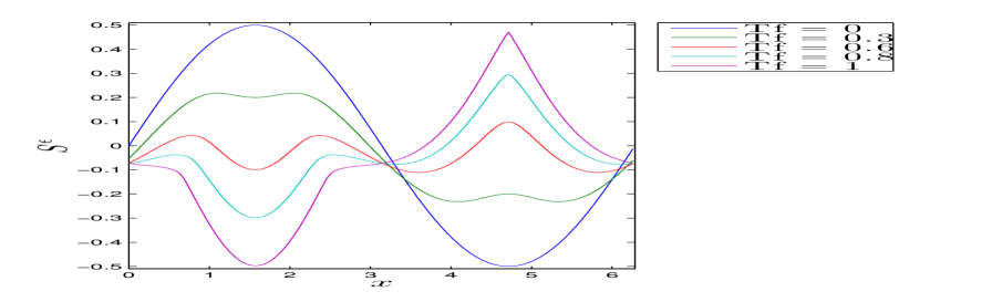
(b) Evolution of the phase $S^{\varepsilon}$ for $\varepsilon=2^{-4}$.

Figure 1. Evolution of the density and of the phase

We first study qualitatively the dynamics, in order to guess what is the time of appearance of the caustics. Figures 1(a) and 1(b) represent the density $|A^{\varepsilon}|^{2}$ and the phase $S^{\varepsilon}$ at times $T_{f}=0$, $0.3$, $0.6$, $0.8$, $1$ for $\varepsilon=2^{-4}$. The caustics appear around $t=0.8$. At time $t=1$, oscillations at other scales than those of the phase can be observed in $|A^{\varepsilon}|^{2}$ whereas $S^{\varepsilon}$ ceases to be smooth. These figures are obtained by using our scheme (1.18) with $N_{x}=2^{8}$ and $N_{t}=T_{f}/h=2^{9}$.

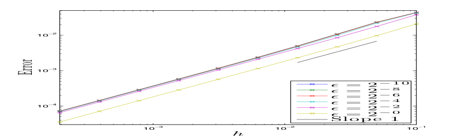
(a) $err_{\rho^{\varepsilon}}(T_{f}=0.2)$ w.r.t $h$, $N_{x}=2^{8}$

(b) $err_{\rho^{\varepsilon}}(T_{f}=0.2)$ w.r.t $\varepsilon$, $N_{x}=2^{8}$

Figure 2. Error on the density $\rho^{\varepsilon}$ for the splitting scheme (1.17) of order $1$ before the caustics: dependence on $\varepsilon$ and on $h$.

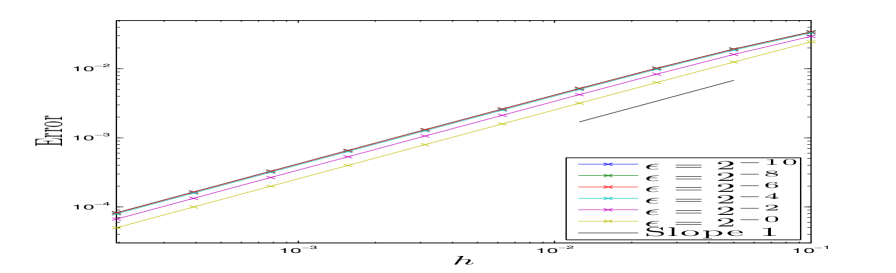
(a) $err_{({S^{\varepsilon}},{A^{\varepsilon}})}(T_{f}=0.2)$ w.r.t $h$, $N_{x}=2^{8}$

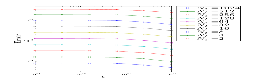
(b) $err_{({S^{\varepsilon}},{A^{\varepsilon}})}(T_{f}=0.2)$ w.r.t $\varepsilon$, $N_{x}=2^{8}$

Figure 3. Error on $({S^{\varepsilon}},{A^{\varepsilon}})$ for the splitting scheme (1.17) of order $1$ before the caustics: dependence on $\varepsilon$ and on $h$.

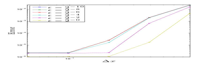
(a) $err_{\rho^{\varepsilon}}(T_{f}=0.2)$ w.r.t $\Delta x$, $N_{t}=2^{15}$

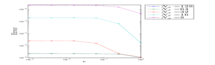
(b) $err_{\rho^{\varepsilon}}(T_{f}=0.2)$ w.r.t $\varepsilon$, $N_{t}=2^{15}$

Figure 4. Error on the density $\rho^{\varepsilon}$ for the splitting scheme (1.17) of order $1$ before the caustics: dependence on $\varepsilon$ and on $\Delta x$.

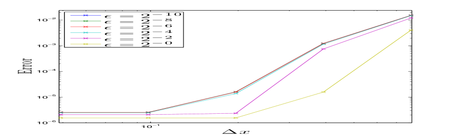
(a) $err_{({S^{\varepsilon}},{A^{\varepsilon}})}(T_{f}=0.2)$ w.r.t $\Delta x$, $N_{t}=2^{15}$

(b) $err_{({S^{\varepsilon}},{A^{\varepsilon}})}(T_{f}=0.2)$ w.r.t $\varepsilon$, $N_{t}=2^{15}$

Figure 5. Error on $({S^{\varepsilon}},{A^{\varepsilon}})$ for the splitting scheme (1.17) of order $1$ before the caustics: dependence on $\varepsilon$ and on $\Delta x$.

Let us now focus on the experiments performed with our first and second-order methods at time $T_{f}=0.2$ before the caustics. We start with the first-order scheme (1.17). Figures 2 and 3 represent the errors on $\rho^{\varepsilon}$ and $({S^{\varepsilon}},{A^{\varepsilon}})$ w.r.t. the time step $h$ for a fixed $N_{x}=2^{7}$. Figures 4 and 5 represent the errors w.r.t. $\Delta x$ for fixed $N_{t}=h/T_{f}=2^{13}$. All these figures illustrate the fact that our scheme is UA with respect to $\varepsilon$, for the quadratic observables as well as for the whole unknown $({S^{\varepsilon}},{A^{\varepsilon}})$ itself. Figures 2 and 3 show that (1.17) is uniformly of order $1$ in time, whereas Figures 4 and 5 show that the convergence is uniformly spectral in space.

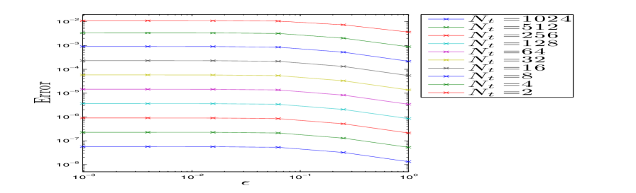
(b) $err_{\rho^{\varepsilon}}(T_{f}=0.2)$ w.r.t $\varepsilon$, $N_{x}=2^{8}$

Figure 6. Error on the density $\rho^{\varepsilon}$ for the splitting scheme (1.18) of order $2$ before the caustics: dependence on $\varepsilon$ and on $h$.

Figures 6 to 9 illustrate the behavior of our second-order scheme (1.18) at $T_{f}=0.2$: here again, it appears that, before the caustics, our method is UA with an order $2$ in time and with spectral in space accuracy.

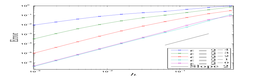
(a) $err_{\rho^{\varepsilon}}(T_{f}=1)$ w.r.t $h$, $N_{x}=2^{8}$

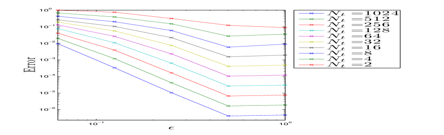
(b) $err_{\rho^{\varepsilon}}(T_{f}=1)$ w.r.t $\varepsilon$, $N_{x}=2^{8}$

Figure 10. Error on $\rho^{\varepsilon}$ for the splitting scheme (1.18) of order $2$ after the caustics, dependence on $\varepsilon$ and on $h$.

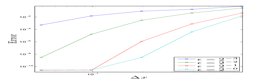
(a) $err_{\rho^{\varepsilon}}(T_{f}=1)$ w.r.t $\Delta x$, $N_{t}=2^{17}$

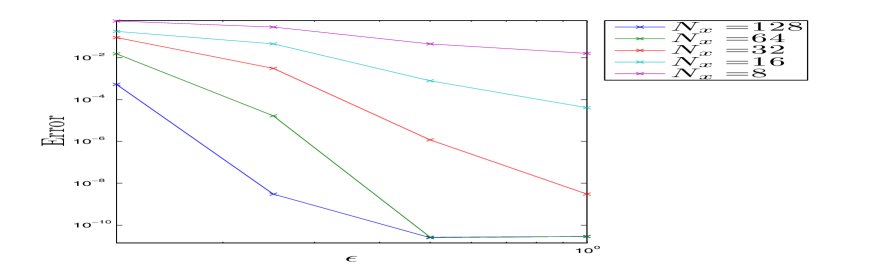
(b) $err_{\rho^{\varepsilon}}(T_{f}=1)$ w.r.t $\varepsilon$, $N_{t}=2^{17}$

Figure 11. Error on $\rho^{\varepsilon}$ for the splitting scheme (1.18) of order $2$ after the caustics, dependence on $\varepsilon$ and on $\Delta x$.

Finally, let us explore the behavior of the splitting methods after caustics, by observing the error on the density $\rho^{\varepsilon}$. Figures 10 and 11 present the same simulations as Figures 2 and 4, except that the final time is now $T_{f}=1$, i.e. we illustrate the behaviors of scheme (1.18) after the caustics. In that case, it appears that our methods are not UA, neither in $h$, nor in $\Delta x$, with respect to $\varepsilon$. Notice that, although it is not UA any longer, our scheme (1.18) still has second-order accuracy in time and spectral accuracy in space (with $\varepsilon$-dependent constants). Recall that the same scheme written on (1.8) would not be usable in the same situation, since $S^{\varepsilon}$ ceases to be regular for $\varepsilon>0$, after the formation of caustics.

Appendix A Proof of Lemma 3.8

A.1. Study of the differentiability of $\varphi^{1}$.

The proof of this lemma is divided in several steps. Let us fix $s>d/2+1$ and $M>0$.

A.1.1. Notations.

For any Banach spaces $E$ and $F$, we denote $\mathscr{L}(E,F)$ the set of continuous linear maps between $E$ and $F$ endowed with the norm

$$\|l\|_{\mathscr{L}(E,F)}=\sup\{\|l(x)\|_{F},\;x\in E,\;\|x\|_{E}\leq 1\}$$

where $\|\cdot\|_{E}$ and $\|\cdot\|_{F}$ are the norms of $E$ and $F$.

Let us define for $u_{0}=(S_{0},A_{0})$

$$\begin{split}\Theta^{1}_{h}\cdot u_{0}=\left(\begin{array}[]{c}\widetilde{S}^{1}_{h}\\ \widetilde{A}^{1}_{h}\end{array}\right)\end{split}$$

the solution of

$$\begin{split}&\partial_{h}\Theta^{1}_{h}=D{\mathcal{N}}_{1}(\varphi^{1}_{h}(u))\cdot\Theta^{1}_{h}\\ &\Theta^{1}_{0}\cdot u_{0}=u_{0}.\end{split}$$

We denote $\Gamma^{1}_{h}=\varphi^{1}_{h}(u+u_{0})-\varphi^{1}_{h}(u)-\Theta^{1}_{h}\cdot u_{0}$,

$$\varphi^{1}_{h}(u)=\left(\begin{array}[]{c}S^{1}_{h}\\ A^{1}_{h}\end{array}\right)\mbox{, }\varphi^{1}_{h}(u+u_{0})=\left(\begin{array}[]{c}\underline{S^{1}_{h}}\\ \underline{A^{1}_{h}}\end{array}\right),$$

$v^{1}_{h}=\nabla S^{1}_{h}$, $\underline{v}^{1}_{h}=\nabla\underline{S}^{1}_{h}$, $\widetilde{v}^{1}_{h}=\nabla\widetilde{S}^{1}_{h}$, $\omega^{1}_{h}=\underline{S}^{1}_{h}-S^{1}_{h}-\widetilde{S}^{1}_{h}$ and $B^{1}_{h}=\underline{A}^{1}_{h}-A^{1}_{h}-\widetilde{A}^{1}_{h}$.

A.1.2. Definition of $h_{8}$.

Lemma 3.5 ensures that for any $u\in B_{s}(2M)$, we have for $h\in[0,h_{5}(2M)]$ that

$$\begin{split}&\|\varphi^{1}_{h}(u)\|_{s}\leq 4M.\end{split}$$ (A.1)

We denote $h_{8}(M)=h_{5}(2M)$.

Let $s^{\prime}\geq s$. If moreover, $u\in\Sigma_{s^{\prime}}$, then we have

$$\begin{split}&\|\varphi^{1}_{h}(u)\|_{s^{\prime}}\leq\exp\left(C_{5}(2M)h\right)\|u\|_{s^{\prime}}.\end{split}$$ (A.2)

A.1.3. Continuity of $\varphi^{1}$.

Let $s^{\prime}\geq s$, $M^{\prime}>0$ and $u_{1},u_{2}\in B_{s}(M)\cap B_{s^{\prime}+1}(M^{\prime})$.

By (LABEL:eq:lemdiffcontrole) and (LABEL:eq:lemdiffcontrole2), we obtain that $\varphi^{1}_{h}(u_{1})$ and $\varphi^{1}_{h}(u_{2})$ are well-defined on $[0,h_{8}]$ and satisfy

$$\|\varphi^{1}_{h}(u_{1})\|_{s^{\prime}+1}+\|\varphi^{1}_{h}(u_{2})\|_{s^{\prime}+1}\leq 2\exp\left(C_{5}(2M)h_{8}\right)M^{\prime}$$

for all $h\in[0,h_{8}].$ By Lemma 3.4 and an integration by parts, we get that there exists $C=C(M,M^{\prime})>0$ such that for all $h\in[0,h_{8}]$

$$\|\varphi^{1}_{h}(u_{1})-\varphi^{1}_{h}(u_{2})\|_{s^{\prime}}\leq C\|u_{1}-u_{2}\|_{s^{\prime}+1}.$$ (A.3)

Moreover, for fixed $u\in B_{s}(M)\cap B_{s^{\prime}+1}(M^{\prime})$, Lemma 3.5 ensures that $h\in[0,h_{8}]\mapsto\varphi^{1}_{h}(u)\in\Sigma_{s^{\prime}}$ is continuous so that

$$(h,u)\in[0,h_{8}]\times\Sigma_{s^{\prime}+1}\mapsto\varphi^{1}_{h}(u)\in\Sigma_{s^{\prime}}$$ (A.4)

is also continuous.

A.1.4. Well-posedness, continuity and estimates on the norm for $\Theta^{1}_{h}$.

Let $s_{2}\geq s$, $M_{2}>0$, $u\in B_{s}(M)\cap B_{s_{2}+1}(M_{2})$ and $u_{0}\in\Sigma_{s_{2}}$. We recall that the function $\Theta^{1}_{h}\cdot u_{0}=:(\widetilde{S}^{1}_{h},\widetilde{A}^{1}_{h})^{T}$ satisfies

$$\begin{split}&\partial_{h}\widetilde{S}^{1}_{h}+\nabla S^{1}_{h}\cdot\nabla\widetilde{S}^{1}_{h}=0\\ &\partial_{h}\widetilde{A}^{1}_{h}+\nabla S^{1}_{h}\cdot\nabla\widetilde{A}^{1}_{h}+\frac{\widetilde{A}^{1}_{h}}{2}\Delta S^{1}_{h}=-\nabla\widetilde{S}^{1}_{h}\cdot\nabla A^{1}_{h}-\frac{A^{1}_{h}}{2}\Delta\widetilde{S}^{1}_{h}+\frac{i}{2}\Delta\widetilde{A}^{1}_{h}\end{split}$$

and $\Theta^{1}_{0}\cdot u_{0}=u_{0}$. The existence and uniqueness of $\widetilde{S}^{1}_{h}$ follows for instance from the method of characteristics. We have

$$\partial_{h}\widetilde{v}^{1}_{h}+\left(v^{1}_{h}\cdot\nabla\right)\widetilde{v}^{1}_{h}=-\left(\widetilde{v}^{1}_{h}\cdot\nabla\right)v^{1}_{h}$$

and Lemma 3.2 with $R=-\left(\widetilde{v}^{1}_{h}\cdot\nabla\right)v^{1}_{h}$ gives us that

$$\begin{split}\partial_{h}\|\widetilde{v}^{1}_{h}\|_{H^{s_{2}+1}}^{2}&\leq C\|\widetilde{v}^{1}_{h}\|_{H^{s_{2}+1}}^{2}\|S^{1}_{h}\|_{H^{s_{2}+3}}\leq C\|\widetilde{v}^{1}_{h}\|_{H^{s_{2}+1}}^{2}\|\varphi^{1}_{h}(u)\|_{s_{2}+1}.\end{split}$$

We also have

$$\partial_{h}\|\widetilde{S}^{1}_{h}\|^{2}_{L^{2}}\leq C\|\widetilde{S}^{1}_{h}\|_{L^{2}}\|\widetilde{S}^{1}_{h}\|_{H^{1}}\|S^{1}_{h}\|_{W^{1,\infty}}$$

so that

$$\partial_{h}\|\widetilde{S}^{1}_{h}\|^{2}_{H^{s_{2}+2}}\leq C\|\widetilde{S}^{1}_{h}\|^{2}_{H^{s_{2}+2}}\|\varphi^{1}_{h}(u)\|_{s_{2}+1}.$$

The existence and uniqueness of $\widetilde{A}^{1}_{h}$ follows from the fact that $\widetilde{w}^{1}_{h}=\widetilde{A}^{1}_{h}\exp\left(iS^{1}_{h}\right)$ satisfies

$$i\partial_{h}\widetilde{w}^{1}_{h}=-\frac{\Delta}{2}\widetilde{w}^{1}_{h}-\left(\nabla\widetilde{S}^{1}_{h}\cdot\nabla A^{1}_{h}+\frac{A^{1}_{h}}{2}\Delta\widetilde{S}^{1}_{h}\right)\exp\left(iS^{1}_{h}\right).$$

Lemma 3.3 with $R=-\nabla\widetilde{S}^{1}_{h}\cdot\nabla A^{1}_{h}-\frac{A^{1}_{h}}{2}\Delta\widetilde{S}^{1}_{h}+\frac{i}{2}\Delta\widetilde{A}^{1}_{h}$ ensures that

$$\begin{split}\partial_{t}\|\widetilde{A}^{1}_{h}\|_{H^{s_{2}}}^{2}&\leq C\|\Theta^{1}_{h}\cdot u_{0}\|_{s_{2}}^{2}\|\varphi^{1}_{h}(u)\|_{s_{2}+1}\end{split}$$

so that

$$\partial_{t}\|\Theta^{1}_{h}\cdot u_{0}\|_{s_{2}}^{2}\leq C\|\Theta^{1}_{h}\cdot u_{0}\|_{s_{2}}^{2}\|\varphi^{1}_{h}(u)\|_{s_{2}+1}.$$

By (LABEL:eq:lemdiffcontrole2) and Gronwall’s Lemma, there is $C_{8}=C_{8}(M,M_{2})>0$ such that for any $h\in[0,h_{8}]$,

$$\|\Theta^{1}_{h}\cdot u_{0}\|_{s_{2}}\leq\exp\left(C_{8}h\right)\|u_{0}\|_{s_{2}}.$$ (A.5)

Using directly the integrations by parts of the proof of Lemmas 3.2 and 3.3, we obtain actually that

$$|\left\langle u_{0},D\mathcal{N}_{1}(\varphi^{1}_{h}(u))\cdot u_{0}\right\rangle_{s_{2}}|\leq C_{8}\|u_{0}\|^{2}_{s_{2}},$$

for all $u_{0}\in\Sigma_{s_{2}}$.

A.1.5. Differentiability of $\varphi^{1}$.

By Lemma 3.5 and equations (1.13), the application

$$h\in[0,h_{8}]\mapsto\varphi^{1}_{h}(u)\in\Sigma_{s_{1}}$$

is differentiable in $h$ for any $u\in B_{s}(M)\cap\Sigma_{s_{1}+2}$.

Let us prove that $\varphi^{1}_{h}$ is differentiable in $u$ and that $\Theta^{1}_{h}$ is its derivative.

Let $M_{1}>0$ and $u,u_{0}\in B_{s}(M)\cap B_{s_{1}+2}(M_{1})$. We have that $u,u+u_{0}\in B_{s}(2M)\cap B_{s_{1}+2}(2M_{1})$. By (LABEL:eq:lemdiffcontrole) and (LABEL:eq:lemdiffcontrole2), we obtain that for all $h\in[0,h_{8}]$,

$$\begin{split}&\|\varphi^{1}_{h}(u)\|_{s_{1}+2}+\|\varphi^{1}_{h}(u+u_{0})\|_{s_{1}+2}\leq 4\exp\left(C_{5}(2M)h\right)M_{1}.\end{split}$$

We have

$$\begin{split}\partial_{h}\nabla\omega^{1}_{h}=-(v^{1}_{h}+\widetilde{v}^{1}_{h})\cdot\nabla(\nabla\omega^{1}_{h})-\left(\nabla\omega^{1}_{h}\cdot\nabla\right)\underline{v^{1}_{h}}-\left(\widetilde{v}^{1}_{h}\cdot\nabla\right)\widetilde{v}^{1}_{h}.\end{split}$$

By Lemma 3.2, we obtain taking $v_{1}=v^{1}_{h}+\widetilde{v}^{1}_{h}$ and

$$R=-\left(\nabla\omega^{1}_{h}\cdot\nabla\right)\underline{v^{1}_{h}}-\left(\widetilde{v}^{1}_{h}\cdot\nabla\right)\widetilde{v}^{1}_{h}$$

that

$$\begin{split}\partial_{t}\|\nabla\omega^{1}_{h}\|_{H^{s_{1}+1}}^{2}&\leq C\|\nabla\omega^{1}_{h}\|_{H^{s_{1}+1}}^{2}\left(\|v^{1}_{h}\|_{H^{s_{1}+1}}+\|\widetilde{v}^{1}_{h}\|_{H^{s_{1}+1}}+\|\underline{v}^{1}_{h}\|_{H^{s_{1}+2}}\right)\\ &\qquad+C\|\nabla\omega^{1}_{h}\|_{H^{s_{1}+1}}\|\widetilde{v}^{1}_{h}\|_{H^{s_{1}+2}}^{2}.\end{split}$$

Moreover, we have

$$\begin{split}\partial_{h}\omega^{1}_{h}=-\frac{1}{2}\left(\nabla\omega^{1}_{h}\cdot(\widetilde{v}^{1}_{h}+v^{1}_{h})+\underline{v}^{1}_{h}\cdot\nabla\omega^{1}_{h}+|\widetilde{v}^{1}_{h}|^{2}\right)\end{split}$$

so that

$$\begin{split}&\partial_{h}\|\omega^{1}_{h}\|^{2}_{H^{s_{1}+2}}\leq\|\Theta^{1}_{h}\cdot u_{0}\|_{s_{1}+1}^{4}\\ &\qquad+C\|\omega^{1}_{h}\|_{H^{s_{1}+2}}^{2}\left(1+\|\varphi^{1}_{h}(u)\|_{s_{1}}+\|\varphi^{1}_{h}(u+u_{0})\|_{s_{1}+1}+\|\Theta^{1}_{h}\cdot u_{0}\|_{s_{1}}\right)\end{split}$$

We also have

$$\begin{split}\partial_{h}B^{1}_{h}=-\nabla\underline{S}^{1}_{h}\cdot\nabla B^{1}_{h}-B^{1}_{h}\frac{\Delta\underline{S}^{1}_{h}}{2}-\nabla\omega^{1}_{h}\cdot\nabla(A^{1}_{h}+\widetilde{A}^{1}_{h})-(A^{1}_{h}+\widetilde{A}^{1}_{h})\frac{\Delta\omega_{h}^{1}}{2}\\ +i\frac{\Delta B^{1}_{h}}{2}-\nabla\widetilde{S}^{1}_{h}\cdot\nabla\widetilde{A}^{1}_{h}-\widetilde{A}^{1}_{h}\frac{\Delta\widetilde{S}^{1}_{h}}{2}\\ \end{split}$$

and Lemma 3.3 ensures taking

$$R=-\nabla\omega^{1}_{h}\cdot\nabla(A^{1}_{h}+\widetilde{A}^{1}_{h})-(A^{1}_{h}+\widetilde{A}^{1}_{h})\frac{\Delta\omega_{h}^{1}}{2}+i\frac{\Delta B^{1}_{h}}{2}-\nabla\widetilde{S}^{1}_{h}\cdot\nabla\widetilde{A}^{1}_{h}-\widetilde{A}^{1}_{h}\frac{\Delta\widetilde{S}^{1}_{h}}{2}$$

that,

$$\begin{split}&\partial_{t}\|B^{1}_{h}\|_{H^{s_{1}}}^{2}\leq\|\Theta^{1}_{h}\cdot u_{0}\|^{4}_{s_{1}+1}\\ &\quad+C\|\Gamma^{1}_{h}\|_{s_{1}}^{2}\left(1+\|\varphi^{1}_{h}(u+u_{0})\|_{s_{1}}+\|\varphi^{1}_{h}(u)\|_{s_{1}+1}+\|\Theta^{1}_{h}\cdot u_{0}\|_{s_{1}+1}\right)\end{split}$$

and

$$\begin{split}&\partial_{h}\|\Gamma^{1}_{h}\|_{s_{1}}^{2}\leq\|\Theta^{1}_{h}\cdot u_{0}\|^{4}_{s_{1}+1}\\ &\quad+C\|\Gamma^{1}_{h}\|_{s_{1}}^{2}\left(1+\|\varphi^{1}_{h}(u+u_{0})\|_{s_{1}+1}+\|\varphi^{1}_{h}(u)\|_{s_{1}+1}+\|\Theta^{1}_{h}\cdot u_{0}\|_{s_{1}+1}\right).\end{split}$$

By (A.5) with $s_{2}=s_{1}+1$ and Gronwall’s Lemma, we get that there exists $C=C(M,M_{1})>0$ such that for all $h\in[h,h_{8}]$,

$$\|\Gamma^{1}_{h}\|_{s_{1}}\leq C\|u_{0}\|_{s_{1}+1}^{2}\leq C\|u_{0}\|_{s_{1}+2}^{2}$$

We proved that for any $h\in[0,h_{8}]$

$$\varphi^{1}_{h}:B_{s}(M)\cap\Sigma_{s_{1}+2}\to\Sigma_{s_{1}}$$

is differentiable in $B_{s}(M)\cap\Sigma_{s_{1}+2}$.

A.1.6. Proof of point (i).

Let us prove that the application

$$(h,u)\in[0,h_{8}]\times\left(B_{s}(M)\cap\Sigma_{s_{1}+4}\right)\mapsto\varphi^{1}_{h}(u)\in\Sigma_{s_{1}}$$

is a $C^{1}$-function.

Using equations (1.13) and (A.4), we get that

$$(h,u)\in[0,h_{8}]\times\left(B_{s}(M)\cap\Sigma_{s_{1}+3}\right)\mapsto\varphi^{1}_{h}(u)\in\Sigma_{s_{1}+2}$$

is continuous so that the partial derivative

$$(h,u)\in[0,h_{8}]\times\left(B_{s}(M)\cap\Sigma_{s_{1}+3}\right)\mapsto\partial_{h}\varphi^{1}_{h}(u)=\mathcal{N}_{1}\varphi^{1}_{h}(u)\in\Sigma_{s_{1}}$$

is also continuous. Let us study the continuity of

$$(h,u)\mapsto\partial_{2}\varphi^{1}_{h}(u).$$

Let $u_{1},u_{2}\in B_{s}(M)\cap B_{s_{1}+2}(M_{1})$. We denote $\varphi^{1}_{h}(u_{i})=(S^{1,i}_{h},A^{1,i}_{h})$ and $\partial_{2}\varphi^{1}_{h}(u_{i})\cdot u_{0}=(\widetilde{S}^{1,i}_{h},\widetilde{A}^{1,i}_{h})$ for $i=1,2$. We have

$$\begin{split}&\partial_{h}\left(\widetilde{S}^{1,1}_{h}-\widetilde{S}^{1,2}_{h}\right)+\nabla S^{1,1}_{h}\cdot\nabla\left(\widetilde{S}^{1,1}_{h}-\widetilde{S}^{1,2}_{h}\right)=-\nabla\left(S^{1,1}_{h}-S^{1,2}_{h}\right)\cdot\nabla\widetilde{S}^{1,2}_{h}\end{split}$$

so that

$$\begin{split}&\partial_{h}\left(\nabla\widetilde{S}^{1,1}_{h}-\nabla\widetilde{S}^{1,2}_{h}\right)+\left(\nabla S^{1,1}_{h}\cdot\nabla\right)\left(\nabla\widetilde{S}^{1,1}_{h}-\nabla\widetilde{S}^{1,2}_{h}\right)\\ &\quad=-\left(\left(\nabla\widetilde{S}^{1,1}_{h}-\nabla\widetilde{S}^{1,2}_{h}\right)\cdot\nabla\right)\left(\nabla S^{1,1}_{h}+\widetilde{S}^{1,2}_{h}\right)\\ &\qquad-\left(\nabla\widetilde{S}^{1,2}_{h}\cdot\nabla\right)\left(\nabla S^{1,1}_{h}-\nabla S^{1,2}_{h}\right).\end{split}$$

By Lemma 3.2 with $v_{1}=\nabla S^{1,1}_{h}$ and

$$\begin{split}R&=-\left(\left(\nabla\widetilde{S}^{1,1}_{h}-\nabla\widetilde{S}^{1,2}_{h}\right)\cdot\nabla\right)\left(\nabla S^{1,1}_{h}+\widetilde{S}^{1,2}_{h}\right)\\ &\quad-\left(\nabla\widetilde{S}^{1,2}_{h}\cdot\nabla\right)\left(\nabla S^{1,1}_{h}-\nabla S^{1,2}_{h}\right),\end{split}$$

which satisfies

$$\begin{split}\|R\|_{H^{s_{1}+1}}&\leq C\|\widetilde{S}^{1,1}_{h}-\widetilde{S}^{1,2}_{h}\|_{H^{s_{1}+2}}\left(\|S^{1,1}_{h}\|_{H^{s_{1}+3}}+\|\widetilde{S}^{1,2}_{h}\|_{H^{s_{1}+3}}\right)\\ &\qquad+C\|S^{1,1}_{h}-S^{1,2}_{h}\|_{H^{s_{1}+3}}\|\widetilde{S}^{1,2}_{h}\|_{H^{s_{1}+2}}\end{split}$$

we obtain that

$$\begin{split}\partial_{t}\|\nabla\widetilde{S}^{1,1}_{h}-\nabla\widetilde{S}^{1,2}_{h}\|_{H^{s_{1}+1}}^{2}&\leq C\|\nabla\widetilde{S}^{1,1}_{h}-\nabla\widetilde{S}^{1,2}_{h}\|_{H^{s_{1}+1}}^{2}\left(\|S^{1,1}_{h}\|_{H^{s_{1}+3}}+\|\widetilde{S}^{1,2}_{h}\|_{H^{s_{1}+3}}\right)\\ &+C\|\nabla\widetilde{S}^{1,1}_{h}-\nabla\widetilde{S}^{1,2}_{h}\|_{H^{s_{1}+1}}\|S^{1,1}_{h}-S^{1,2}_{h}\|_{H^{s_{1}+3}}\|\widetilde{S}^{1,2}_{h}\|_{H^{s_{1}+2}}.\end{split}$$

Moreover, we have

$$\begin{split}&\partial_{t}\|\widetilde{S}^{1,1}_{h}-\widetilde{S}^{1,2}_{h}\|^{2}_{L^{2}}\\ &\;\leq C\|\widetilde{S}^{1,1}_{h}-\widetilde{S}^{1,2}_{h}\|_{L^{2}}\left(\|\widetilde{S}^{1,1}_{h}-\widetilde{S}^{1,2}_{h}\|_{H^{1}}\|S^{1,1}_{h}\|_{W^{1,\infty}}+\|S^{1,1}_{h}-S^{1,2}_{h}\|_{H^{1}}\|\widetilde{S}^{1,2}_{h}\|_{W^{1,\infty}}\right)\end{split}$$

so that

$$\begin{split}\partial_{t}\|\widetilde{S}^{1,1}_{h}-\widetilde{S}^{1,2}_{h}\|_{H^{s_{1}+2}}^{2}&\leq C\|\widetilde{S}^{1,1}_{h}-\widetilde{S}^{1,2}_{h}\|_{H^{s_{1}+2}}^{2}\left(\|S^{1,1}_{h}\|_{H^{s_{1}+3}}+\|\widetilde{S}^{1,2}_{h}\|_{H^{s_{1}+3}}\right)\\ &\qquad+C\|\widetilde{S}^{1,1}_{h}-\widetilde{S}^{1,2}_{h}\|_{H^{s_{1}+2}}\|S^{1,1}_{h}-S^{1,2}_{h}\|_{H^{s_{1}+3}}\|\widetilde{S}^{1,2}_{h}\|_{H^{s_{1}+2}}.\end{split}$$

We also have

$$\begin{split}&\partial_{h}\left(\widetilde{A}^{1,1}_{h}-\widetilde{A}^{1,2}_{h}\right)+\nabla S^{1,1}_{h}\cdot\nabla\left(\widetilde{A}^{1,1}_{h}-\widetilde{A}^{1,2}_{h}\right)+\left(\widetilde{A}^{1,1}_{h}-\widetilde{A}^{1,2}_{h}\right)\frac{\Delta S^{1,1}_{h}}{2}\\ &\quad=-\nabla\left(S^{1,1}_{h}-S^{1,2}_{h}\right)\cdot\nabla\widetilde{A}^{1,2}_{h}-\frac{\widetilde{A}^{1,2}_{h}}{2}\Delta\left(S^{1,1}_{h}-S^{1,2}_{h}\right)\\ &\qquad-\nabla\left(\widetilde{S}^{1,1}_{h}-\widetilde{S}^{1,2}_{h}\right)\cdot\nabla A^{1,1}_{h}-\frac{A^{1,1}_{h}}{2}\Delta\left(\widetilde{S}^{1,1}_{h}-\widetilde{S}^{1,2}_{h}\right)\\ &\qquad-\nabla\widetilde{S}^{1,2}_{h}\cdot\nabla\left(A^{1,1}_{h}-A^{1,2}_{h}\right)-\frac{\left(A^{1,1}_{h}-A^{1,2}_{h}\right)}{2}\Delta\widetilde{S}^{1,2}_{h}+\frac{i}{2}\Delta\left(\widetilde{A}^{1,1}_{h}-\widetilde{A}^{1,2}_{h}\right).\end{split}$$

Using Lemma 3.3 with $v_{1}=\nabla S^{1,1}_{h}$ and

$$\begin{split}&R=-\nabla\left(S^{1,1}_{h}-S^{1,2}_{h}\right)\cdot\nabla\widetilde{A}^{1,2}_{h}-\frac{\widetilde{A}^{1,2}_{h}}{2}\Delta\left(S^{1,1}_{h}-S^{1,2}_{h}\right)\\ &\qquad-\nabla\left(\widetilde{S}^{1,1}_{h}-\widetilde{S}^{1,2}_{h}\right)\cdot\nabla A^{1,1}_{h}-\frac{A^{1,1}_{h}}{2}\Delta\left(\widetilde{S}^{1,1}_{h}-\widetilde{S}^{1,2}_{h}\right)\\ &\qquad-\nabla\widetilde{S}^{1,2}_{h}\cdot\nabla\left(A^{1,1}_{h}-A^{1,2}_{h}\right)-\frac{\left(A^{1,1}_{h}-A^{1,2}_{h}\right)}{2}\Delta\widetilde{S}^{1,2}_{h}+\frac{i}{2}\Delta\left(\widetilde{A}^{1,1}_{h}-\widetilde{A}^{1,2}_{h}\right).\end{split}$$

which satisfies

$$\begin{split}&\operatorname{Re}\left\langle\Lambda^{s_{1}}\left(\widetilde{A}^{1,1}_{h}-\widetilde{A}^{1,2}_{h}\right),\Lambda^{s_{1}}R\right\rangle\\ &\quad\leq C\|\widetilde{A}^{1,1}_{h}-\widetilde{A}^{1,2}_{h}\|_{H^{s_{1}}}\|S^{1,1}_{h}-S^{1,2}_{h}\|_{H^{s_{1}+2}}\|\widetilde{A}^{1,2}_{h}\|_{H^{s_{1}+1}}\\ &\qquad+C\|\widetilde{A}^{1,1}_{h}-\widetilde{A}^{1,2}_{h}\|_{H^{s_{1}}}\|\widetilde{S}^{1,1}_{h}-\widetilde{S}^{1,2}_{h}\|_{H^{s_{1}+2}}\|A^{1,1}_{h}\|_{H^{s_{1}+1}}\\ &\qquad+C\|\widetilde{A}^{1,1}_{h}-\widetilde{A}^{1,2}_{h}\|_{H^{s_{1}}}\|A^{1,1}_{h}-A^{1,2}_{h}\|_{H^{s_{1}+1}}\|\widetilde{S}^{1,2}_{h}\|_{H^{s_{1}+2}}\end{split}$$

we obtain that

$$\begin{split}&\partial_{h}\|\left(\partial_{2}\varphi^{1}_{h}(u_{1})-\partial_{2}\varphi^{1}_{h}(u_{2})\right)\cdot u_{0}\|_{{s_{1}}}^{2}\\ &\qquad\leq C\|\left(\partial_{2}\varphi^{1}_{h}(u_{1})-\partial_{2}\varphi^{1}_{h}(u_{2})\right)\cdot u_{0}\|^{2}_{s_{1}}\left(\|\varphi^{1}_{h}(u_{1})\|_{s_{1}+1}+\|\partial_{2}\varphi^{1}_{h}(u_{2})\cdot u_{0}\|_{s_{1}+1}\right)\\ &\qquad+C\|\left(\partial_{2}\varphi^{1}_{h}(u_{1})-\partial_{2}\varphi^{1}_{h}(u_{2})\right)\cdot u_{0}\|_{s_{1}}\|\varphi^{1}_{h}(u_{1})-\varphi^{1}_{h}(u_{2})\|_{s_{1}+1}\|\partial_{2}\varphi^{1}_{h}(u_{2})\cdot u_{0}\|_{s_{1}+1}.\end{split}$$

Let us recall that $u_{1},u_{2}\in B_{s}(M)\cap B_{s_{1}+2}(M_{1})$. By (LABEL:eq:lemdiffcontrole2), (A.3) and (A.5) with $s_{2}=s_{1}$ and Gronwall’s Lemma, we get that for all $h\in[0,h_{8}]$,

$$u\in B_{s}(M)\cap\Sigma_{s_{1}+2}\mapsto\partial_{2}\varphi^{1}_{h}(u)\in\mathscr{L}(\Sigma_{s_{1}+2},\Sigma_{s_{1}})$$

is continuous. Hence, we obtain that

$$\begin{split}&(h,u)\in[0,h_{8}]\times\left(B_{s}(M)\cap\Sigma_{s_{1}+3}\right)\mapsto(\partial_{2}\varphi^{1}_{h}(u),\partial_{h}\varphi^{1}_{h}(u))\in\mathscr{L}(\Sigma_{s_{1}+3},\Sigma_{s_{1}})\times\Sigma_{s_{1}}\end{split}$$

is continuous and the result follows.

A.2. Study of the differentiability of $\varphi^{2}$ and $\varphi^{3}$.

Let $u,u_{0}\in\Sigma_{s}$. Since $\mathcal{N}_{2}$ is linear, we have that

$$\Theta^{2}_{h}\cdot u_{0}=\varphi^{2}_{h}(u_{0}),$$

$\varphi^{2}_{h}$ is differentiable on $\Sigma_{s}$ and for any $h\geq 0$,

$$\begin{split}&\|\partial_{2}\varphi^{2}_{h}(u)\cdot u_{0}\|_{s}=\|\varphi^{2}_{h}(u_{0})\|_{s}=\|u_{0}\|_{s},\\ &|\left\langle u_{0},D\mathcal{N}_{2}(\varphi^{2}_{h}(u))\cdot u_{0}\right\rangle_{s}|\leq C\|u_{0}\|^{2}_{s}.\end{split}$$

and the result follows. We easily prove that $\varphi^{3}_{i}$ is differentiable, that for any $h\geq 0$, $\Theta^{3}_{h}\cdot u_{0}=u_{0}$, that

$$\|\Theta^{3}_{h}\cdot u_{0}\|_{s}=\|\Theta^{3}_{0}\cdot u_{0}\|_{s}=\|u_{0}\|_{s}.$$

and

$$|\left\langle\chi,\left(D\mathcal{N}_{3}(\varphi^{3}_{h}(u))\cdot\chi\right)\right\rangle_{s}|\leq C\|\chi\|^{2}_{s},$$

for all $\chi\in\Sigma_{s}$.

(a) Evolution of the density $|A^{\varepsilon}|^{2}$ for $\varepsilon=2^{-4}$.

(a) $err_{\rho^{\varepsilon}}(T_{f}=0.2)$ w.r.t $h$, $N_{x}=2^{8}$

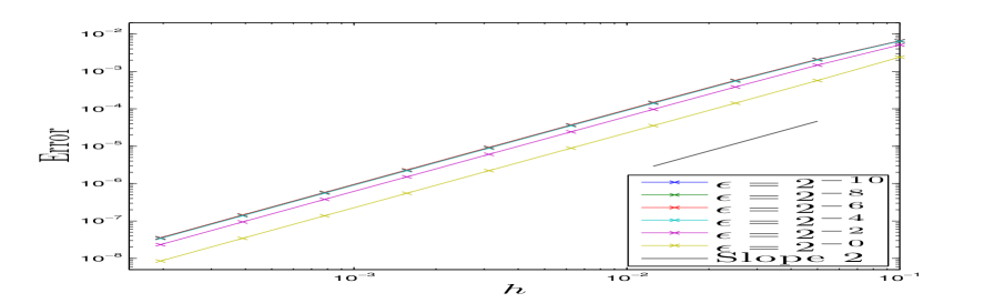
(a) $err_{({S^{\varepsilon}},{A^{\varepsilon}})}(T_{f}=0.2)$ w.r.t $h$, $N_{x}=2^{8}$

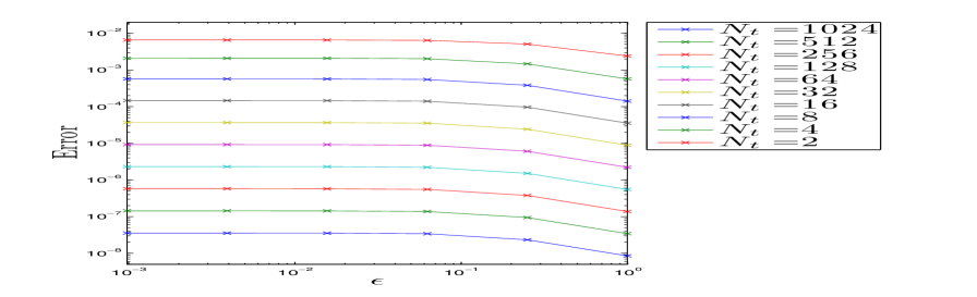
(b) $err_{({S^{\varepsilon}},{A^{\varepsilon}})}(T_{f}=0.2)$ w.r.t $\varepsilon$, $N_{x}=2^{8}$

Figure 7. Error on $({S^{\varepsilon}},{A^{\varepsilon}})$ for the splitting scheme (1.18) of order $2$ before the caustics: dependence on $\varepsilon$ and on $h$.

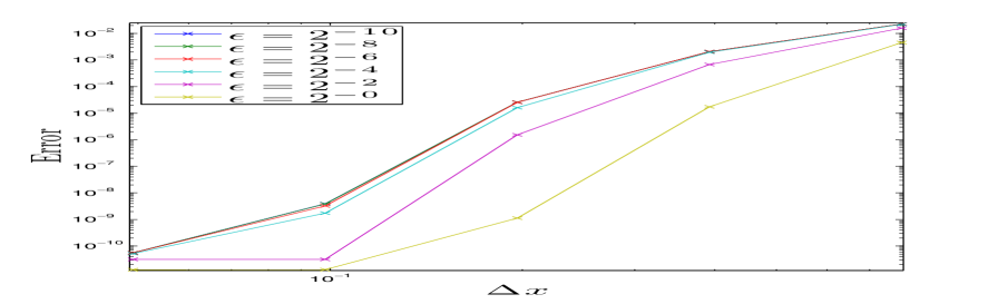
(a) $err_{\rho^{\varepsilon}}(T_{f}=0.2)$ w.r.t $\Delta x$, $N_{t}=2^{15}$

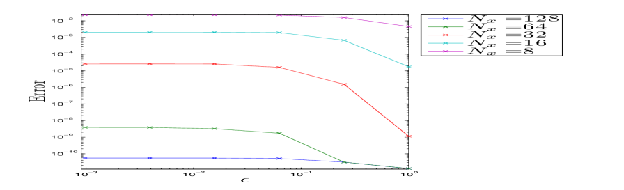
(b) $err_{\rho^{\varepsilon}}(T_{f}=0.2)$ w.r.t $\varepsilon$, $N_{t}=2^{15}$

Figure 8. Error on $\rho^{\varepsilon}$ for the splitting scheme (1.18) of order $2$ before the caustics: dependence on $\varepsilon$ and on $\Delta x$.

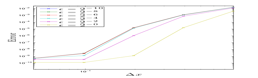
(a) $err_{({S^{\varepsilon}},{A^{\varepsilon}})}(T_{f}=0.2)$ w.r.t $\Delta x$, $N_{t}=2^{15}$

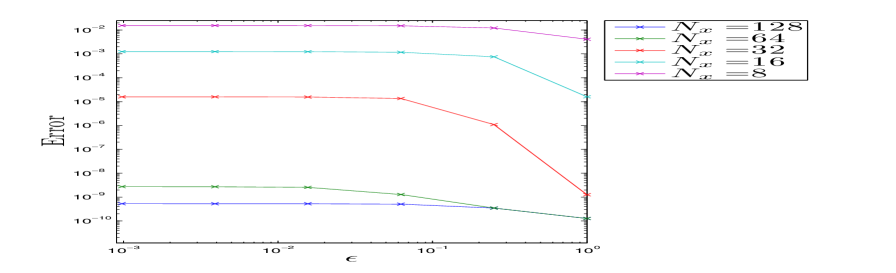
(b) $err_{({S^{\varepsilon}},{A^{\varepsilon}})}(T_{f}=0.2)$ w.r.t $\varepsilon$, $N_{t}=2^{15}$

Figure 9. Error on $({S^{\varepsilon}},{A^{\varepsilon}})$ for the splitting scheme (1.18) of order $2$ before the caustics: dependence on $\varepsilon$ and on $\Delta x$.

References

- [1] G. D. Akrivis, Finite difference discretization of the cubic Schrödinger equation, IMA J. Numer. Anal., 13 (1993), pp. 115–124.
- [2] W. Auzinger, H. Hofstätter, O. Koch, and M. Thalhammer, Defect-based local error estimators for splitting methods, with application to Schrödinger equations, Part III: The nonlinear case, J. Comput. Appl. Math., 273 (2015), pp. 182–204.
- [3] P. Bader, A. Iserles, K. Kropielnicka, and P. Singh, Effective approximation for the semiclassical Schrödinger equation, Foundations of Computational Mathematics, 14 (2014), pp. 689–720.
- [4] , Efficient methods for linear Schrödinger equation in the semiclassical regime with time-dependent potential, Proc. A., 472 (2016), pp. 20150733, 18.
- [5] W. Bao, S. Jin, and P. A. Markowich, On time-splitting spectral approximations for the Schrödinger equation in the semiclassical regime, Journal of Computational Physics, 175 (2002), pp. 487–524.
- [6] W. Bao, S. Jin, and P. A. Markowich, Numerical study of time-splitting spectral discretizations of nonlinear Schrödinger equations in the semiclassical regimes, SIAM Journal on Scientific Computing, 25 (2003), pp. 27–64.
- [7] C. Besse, Relaxation scheme for time dependent nonlinear Schrödinger equations, in Mathematical and Numerical Aspects of Wave Propagation (Santiago de Compostela, 2000), SIAM, Philadelphia, PA, 2000, pp. 605–609.
- [8] C. Besse, B. Bidégaray, and S. Descombes, Order estimates in time of splitting methods for the nonlinear Schrödinger equation, SIAM Journal on Numerical Analysis, 40 (2002), pp. 26–40 (electronic).
- [9] C. Besse, R. Carles, and F. Méhats, An asymptotic preserving scheme based on a new formulation for NLS in the semiclassical limit, Multiscale Modeling and Simulation, 11 (2013), pp. 1228–1260.
- [10] S. Blanes, F. Casas, P. Chartier, and A. Murua, Optimized high-order splitting methods for some classes of parabolic equations, Mathematics of Computation, 82 (2012), pp. 1559–1576.
- [11] M. Caliari, A. Ostermann, and C. Piazzola, A splitting approach for the magnetic Schrödinger equation, J. Comput. Appl. Math., 316 (2017), pp. 74–85.
- [12] R. Carles, Semi-classical analysis for nonlinear Schrödinger equations, World Scientific, 2008.
- [13] , On Fourier time-splitting methods for nonlinear Schrödinger equations in the semiclassical limit, SIAM Journal on Numerical Analysis, 51 (2013), pp. 3232–3258.
- [14] R. Carles, R. Danchin, and J.-C. Saut, Madelung, Gross-Pitaevskii and Korteweg, Nonlinearity, 25 (2012), pp. 2843–2873.
- [15] P. Degond, S. Gallego, and F. Méhats, An asymptotic preserving scheme for the Schrödinger equation in the semiclassical limit, Comptes Rendus Mathématique. Académie des Sciences. Paris, 345 (2007), pp. 531–536.
- [16] M. Delfour, M. Fortin, and G. Payre, Finite-difference solutions of a nonlinear Schrödinger equation, J. Comput. Phys., 44 (1981), pp. 277–288.
- [17] S. Descombes and M. Thalhammer, An exact local error representation of exponential operator splitting methods for evolutionary problems and applications to linear Schrödinger equations in the semi-classical regime, BIT. Numerical Mathematics, 50 (2010), pp. 729–749.
- [18] , The Lie-Trotter splitting for nonlinear evolutionary problems with critical parameters: A compact local error representation and application to nonlinear Schrödinger equations in the semiclassical regime, IMA Journal of Numerical Analysis, 33 (2013), pp. 722–745.
- [19] L. Einkemmer and A. Ostermann, On the error propagation of semi-Lagrange and Fourier methods for advection problems, Comput. Math. Appl., 69 (2015), pp. 170–179.
- [20] L. C. Evans, Partial differential equations, Providence, Rhode Land: American Mathematical Society, 1998.
- [21] E. Faou, V. Gradinaru, and C. Lubich, Computing semiclassical quantum dynamics with Hagedorn wavepackets, SIAM Journal on Scientific Computing, 31 (2009), pp. 3027–3041.
- [22] E. Faou and C. Lubich, A Poisson integrator for Gaussian wavepacket dynamics, Comput. Vis. Sci., 9 (2006), pp. 45–55.
- [23] V. Gradinaru and G. A. Hagedorn, Convergence of a semiclassical wavepacket based time-splitting for the Schrödinger equation, Numerische Mathematik, 126 (2014), pp. 53–73.
- [24] R. N. H. Holden H., Lubich C., Operator splitting for partial differential equations with Burgers nonlinearity, Math. Comp., 82 (2012), p. 13.
- [25] S. Jin, P. Markowich, and C. Sparber, Mathematical and computational methods for semiclassical Schrödinger equations, Acta Numerica, 20 (2011), pp. 121–209.
- [26] O. Karakashian, G. D. Akrivis, and V. A. Dougalis, On optimal order error estimates for the nonlinear Schrödinger equation, SIAM Journal on Numerical Analysis, 30 (1993), pp. 377–400.
- [27] T. Kato, Perturbation Theory for linear operators, Classics in Mathematics, Springer-Verlag, Berlin, 1995. Reprint of the 1980 edition.
- [28] T. Kato and G. Ponce, Commutator estimates and the Euler and Navier-Stokes equations, Comm. Pure Appl. Math., 41 (1988), pp. 891–907.
- [29] C. Lubich, On splitting methods for Schrödinger-Poisson and cubic nonlinear Schrödinger equations, Mathematics of Computation, 77 (2008), pp. 2141–2153.
- [30] E. Madelung, Quanten Theorie in Hydrodynamischer Form, Zeit. F. Physik, 40 (1927), pp. 322–326.
- [31] D. Pathria and J. L. Morris, Pseudo-spectral solution of nonlinear Schrödinger equations, Journal of Computational Physics, 87 (1990), pp. 108–125.
- [32] A. Pazy, Semigroups of Linear Operators and Applications to Partial Differential Equations, vol. 44 of Applied Mathematical Sciences, Springer-Verlag, New York, 1983.
- [33] J. M. Sanz-Serna and J. G. Verwer, Conservative and nonconservative schemes for the solution of the nonlinear Schrödinger equation, IMA Journal of Numerical Analysis, 6 (1986), pp. 25–42.
- [34] J. A. C. Weideman and B. M. Herbst, Split-step methods for the solution of the nonlinear Schrödinger equation, SIAM Journal on Numerical Analysis, 23 (1986), pp. 485–507.
- [35] L. Wu, Dufort-Frankel-type methods for linear and nonlinear Schrödinger equations, SIAM J. Numer. Anal., 33 (1996), pp. 1526–1533.
- [36] H. Yoshida, Construction of higher order symplectic integrators, Phys. Lett. A, 150 (1990), pp. 262–268.