Metastable and scaling regimes of a one-dimensional Kawasaki dynamics

Abstract

We investigate the large-time scaling regimes arising from a variety of metastable structures in a chain of Ising spins with both first- and second-neighbor couplings while subject to a Kawasaki dynamics. Depending on the ratio and sign of these former, different dynamic exponents are suggested by finite-size scaling analyses of relaxation times. At low but nonzero-temperatures these are calculated via exact diagonalizations of the evolution operator in finite chains under several activation barriers. In the absence of metastability the dynamics is always diffusive.

I Introduction

Systems whose thermodynamic parameters are drastically changed give rise to highly nonlinear and far from equilibrium processes that have been intensively studied for decades in various contexts Puri . These may range from binary fluids to alloys and spin systems exhibiting a disordered phase at high temperatures, whilst having two or more ordered phases below a critical point Puri ; Puri2 . There is already a vast body of research studying such nonequilibrium problems in terms of kinetic Ising models Puri ; Puri2 ; Kawasaki under both Glauber and Kawasaki dynamics Glauber ; Kawasaki2 , respectively associated with the so called models $A$ and $B$ in the terminology of critical dynamic theories Hohenberg . After a quench to a subcritical temperature these dynamics attempt to minimize the interfacial energy between different equilibrium domains which therefore grow and coarsen with time. At late stages the spreading of domains is such that if their typical lengths are rescaled by a factor $t^{-1/z}$ the domain patterns at different times will be statistically similar. Here, the scaling or dynamic exponent $z$ is characteristic of the universality class to which the dynamic belongs, and is usually independent of the spatial dimensionality but sensitive to conservation laws (see, e.g. Puri ; Puri2 ; Hohenberg ; Redner and references therein).

For one-dimensional (1D) systems these dynamics are also amenable to experimental probe Privman . In particular, the magnetic relaxation of synthesized molecular chains with strong Ising anisotropy exp was considered in the framework of a Glauber dynamics with both first- and second-neighbor interactions $J_{1},J_{2}$ Pini . In that regard, recently it was suggested that weak competing regimes in the low but nonzero-temperature limit ($T=0^{+}$) give rise to an almost ballistic dynamic exponent ($z\simeq 1$) Grynberg rather than the usual diffusive value of $z=2$ Puri ; Glauber . Irrespective of how small the frustration might be, note that for $0<-J_{2}<|J_{1}|$ such discontinuous scaling behavior is also accompanied by the sudden appearance of a large basin of metastable states Redner2 . When it comes to the ferromagnetic Kawasaki dynamics, these latter already exist for $J_{2}=0$ and are characterized by kinks or domain walls separated by two or more lattice spacings Robin ; Redner . In that situation the mean density of kinks reaches a finite value details , and so the average size of metastable domains can not but remain bounded. At zero temperature the dynamics rapidly gets stuck in these states  -thus preventing the system to reach equilibrium-  but for $T=0^{+}$ their structure is at the origin of the $t^{1/3}\!$ growth of domain length scales Robin ; details . Despite metastability, note that as long as temperature is held finite, no matter how small, the dynamics is still ergodic and eventually the equilibrium state is accessible.

Continuing the development initiated in Ref. Grynberg , in this work we further investigate the metastable effects brought about by second neighbor couplings on the scaling regimes of this typical phase separation dynamics. As we shall see, for $J_{2}\neq 0$ there are new metastable scenarios and activation barriers that come into play, ultimately affecting the large time kinetics in the low temperature limit.

Following the methodology of Ref. Grynberg , first we will construct and diagonalize numerically the kink evolution operator associated to the master equation Kampen of this dynamics in finite chains. This will enable us to determine the relaxation time ($\tau$) of these processes from the spectral gaps of that Liouvillian operator. As is known, in nearing a critical point those time scales diverge with the equilibrium correlation length as $\tau\propto\xi^{z}$ Hohenberg , which in the present context also grows unbounded in the limit of $T\to 0^{+}$ (except for $J_{2}=-|J_{1}|/2\,$ where the ground state is highly degenerate and $\xi$ remains finite Tanaka  ). On the other hand, in a system of typical length $L$ evidently $\xi$ can not grow beyond that scale; hence in practice it is customary to trade that scaling relation by the finite-size behavior

$$\tau\propto L^{z},$$ (1)

provided $L$ is taken sufficiently large Henkel . Thus, once armed with the above referred spectral gaps we will aim at obtaining dynamic exponents from this finite-size scaling relation across a host of metastable situations. At low but nonzero-temperatures, however notice that owing to the presence of Arrhenius activation energies the time scales involved are unbounded even for finite systems (cf. Sec. IV).

The structure of this work is organized as follows. In Sec. II we recast the master equation of these stochastic processes in terms of a quantum spin analogy that readily lends itself to evaluate the low lying levels of the associated evolution operator. Owing to detailed balance Kampen this latter can be brought to a symmetric representation by means of simple nonunitary spin transformations, thus simplifying the subsequent numerical analysis. Sec. III describes various metastable regimes while attempting to identify their decay patterns and activation barriers. Calculational details regarding the proliferation rates of these states with the system size are relegated to Appendix A. In Sec. IV we evaluate numerically the spectrum gaps of finite chains using standard recursive techniques Lanczos which yield clear Arrhenius trends for relaxation times at low temperature regimes. This provides a sequence of finite-size approximants to dynamic exponents which are then combined with extrapolations to the thermodynamic limit Henkel ; Guttmann . Finally, Sec. V contains a summarizing discussion along with some remarks on open issues and prospects of future work.

II Dynamics and operators

Let us consider the Kawasaki dynamics in a chain of Ising spins ($S=\pm 1$) coupled with both first- and second-neighbor interactions $J_{1},J_{2}$, thus setting energy configurations

$$E_{S}=-J_{1}\sum_{i}S_{i}\,S_{i+1}-J_{2}\sum_{i}S_{i}\,S_{i+2}\,,$$ (2)

while in contact with a heat bath at temperature $T$. Here, frustration arises when combining antiferromagnetic (AF) $J_{2}$ couplings ($J_{2}<0$) with $J_{1}$ exchanges of any sign. In particular, for $-J_{2}/|J_{1}|>1/2$ the ground state consists of consecutive pairs of oppositely oriented spins ($\cdots\bullet\bullet\circ\circ\cdots$), while for $0\leq-J_{2}/|J_{1}|<1/2$ the ordering is F or AF depending on the respective sign of $J_{1}$. For $J_{2}>0$ there is no frustration and the order type is also set by $J_{1}$. Unless otherwise stated, periodic boundary conditions (PBC) and a vanishing magnetization will be assumed throughout.

The bath is represented as causing the Ising states $|S\,\rangle=|S_{1},\,\dots\,,S_{L}\rangle$ to fluctuate by exchanges of nearest neighbor (NN) spin pairs chosen randomly from $L$ locations. To enforce the system to relax towards the Boltzmann distribution $P_{B}(S)\propto e^{-E_{S}/k_{B}T}$, the transition probability rates per unit time $W(S\to S^{\prime})$ between two configurations $|S\rangle,|S^{\prime}\rangle$ (here differing just in an exchanged pair of NN spins), are chosen to satisfy the detailed balance condition Kampen

$$P_{B}(S)\,W(S\to S^{\prime})=P_{B}(S^{\prime})\,W(S^{\prime}\to S)\,,$$ (3)

(also, see its role by the end of Sec. II A). However, detailed balance itself cannot determine entirely the form of such rates, thus in what follows we take up the common choice used in the context of kinetic Ising models, namely Kubo

$$W(S\to S^{\prime})=\frac{\alpha}{2}\Big{\{}\,1-\tanh\Big{[}\,\frac{\beta}{2}\,\big{(}E_{S^{\prime}}-E_{S}\big{)}\Big{]}\,\Big{\}}\,,$$ (4)

where $\alpha^{-1}$ just sets the time scale of the microscopic process, and is hereafter set to 1. Also, from now on temperatures are measured in energy units, or, equivalently, the Boltzmann constant in $\beta\equiv 1/(k_{B}T)$ is taken equal to unity. In the specific case of spin exchanges, say at locations $i,i+1$, clearly from Eq. (2) the above energy differences reduce to $\frac{1}{2}\,(S_{i}-S_{i+1})\left[\,(J_{1}-J_{2})\left(\,S_{i-1}-S_{i+2},\right)+J_{2}\left(\,S_{i-2}-S_{i+3}\,\right)\,\right]$. Thus, after introducing the parameters

$$P = 2\,(K_{1}-K_{2})\,,\,\;\;Q=2\,(K_{1}-2K_{2})\,,$$ (5a)

$$A_{\pm} = \pm\frac{1}{8}\left(\,\tanh\,2K_{1}-\tanh\,Q\,\right)+\frac{1}{4}\tanh\,2K_{2}\,,$$ (5b)

$$B_{\pm} = \pm\frac{1}{8}\left(\,\tanh\,2K_{1}+\tanh\,Q\,\right)+\frac{1}{4}\tanh P\,,$$ (5c)

($K_{1,2}\equiv J_{1,2}/T$) and using basic properties of hyperbolic functions, it is a straightforward matter to verify that the exchange rates $W(S_{i},\,S_{i+1})$ associated to those locations actually deploy multi-spin terms of the form

$$W\left(S_{i},\,S_{i+1}\right) = \frac{1}{4}\,\big{(}1-S_{i}\,S_{i+1}\big{)}\,-\frac{1}{4}\,\big{(}S_{i}-S_{i+1}\big{)}$$ (6)

$$\times \Big{[}\big{(}\,A_{{}_{+}}+A_{{}_{-}}\;S_{i-1}\;S_{i+2}\big{)}\,\big{(}S_{i-2}-S_{i+3}\big{)}+\big{(}B_{{}_{+}}+B_{{}_{-}}\;S_{i-2}\;S_{i+3}\big{)}\,\big{(}S_{i-1}-S_{i+2}\big{)}\Big{]}\,,$$

which already anticipate the type of many-body interactions to be found later on in the evolution operator of Sec. II A. Here, the factors $(1-S_{i}\,S_{i+1})$ and $(S_{i}-S_{i+1})$ ensure vanishing rates for parallel spins while contributing to reproduce Eq. (4) for antiparallel ones. Also, note that although the standard case of $J_{2}=0$ is left with terms of just two-spin interactions, its dynamics is not yet amenable for exact analytic treatments at $T>0$ Godreche .

The range of the sites involved in Eq. (6), or equivalently, in the energy differences of Eq. (4), basically distinguishes between eight situations of spin exchanges. For later convenience we now regroup them in two sets of dual events in which kinks or ferromagnetic domain walls are thought of as hard core particles $A$ undergoing pairing $\emptyset+A+\emptyset\,\rightleftarrows\,A+A+A$, and diffusion $A+A+\emptyset\,\rightleftarrows\,\emptyset+A+A$ processes, as schematized in Table 1. Its columns also summarize the information needed to construct the operational form of the dynamics, while allowing to infer the variety of metastable structures alluded to in Sec. I. In what follows we turn to the first of these issues, and defer the discussion of the second to Sec. III.

Pairing    $\emptyset+A+\emptyset\;\,\rightleftarrows\;A+A+A$	Rate $(\rightleftarrows)$	$\beta\Delta E\,(\rightleftarrows)$	S element	Projector
$\bullet\;\bullet\;{\color[rgb]{0,0,1}\bullet\,|\,\circ}\,\circ\,\circ\;\;\;\rightleftarrows\;\;\,\bullet\;\bullet{\color[rgb]{0,0,1}|\circ|\bullet|}\circ\;\circ$	$\frac{1}{2}(1\mp\tanh 2K_{{}_{\!1}})$	$\pm 4K_{{}_{\!1}}$	$\frac{1}{2}\,{\rm sech}\,2K_{{}_{\!1}}$	${\cal P}^{(1)}$
$\circ\,|\bullet\,{\color[rgb]{0,0,1}\bullet\,|\,\circ}\,\circ\,\circ\;\;\;\rightleftarrows\;\;\,\circ\,|\bullet{\color[rgb]{0,0,1}|\circ|\bullet|}\circ\,\circ$	$\frac{1}{2}(1\mp\tanh P)$	$\pm 2P$	$\frac{1}{2}\,{\rm sech}\,P$	${\cal P}^{(2)}$
$\,\bullet\;\bullet\;{\color[rgb]{0,0,1}\bullet\,|\,\circ\,}\circ|\,\bullet\;\;\,\rightleftarrows\;\;\bullet\;\bullet{\color[rgb]{0,0,1}|\circ|\bullet|}\circ|\,\bullet$	$\frac{1}{2}(1\mp\tanh P)$	$\pm 2P$	$\frac{1}{2}\,{\rm sech}\,P$	${\cal P}^{(3)}$
$\,\circ\,|\bullet\,{\color[rgb]{0,0,1}\bullet\,|\,\circ}\,\circ|\,\bullet\;\;\,\rightleftarrows\;\;\circ\,|\bullet{\color[rgb]{0,0,1}|\circ|\bullet|}\circ|\,\bullet$	$\frac{1}{2}(1\mp\tanh Q)$	$\pm 2Q$	$\frac{1}{2}\,{\rm sech}\,Q$	${\cal P}^{(4)}$
Diffusion    $A+A+\emptyset\;\,\rightleftarrows\;\emptyset+A+A$	Rate $(\rightleftarrows)$	$\beta\Delta E\,(\rightleftarrows)$	S element	Projector
$\circ\;\circ{\color[rgb]{0,0,1}|\bullet|\;\circ}\,\circ\,\circ\;\;\;\rightleftarrows\;\;\circ\;\circ\;{\color[rgb]{0,0,1}\circ\,|\bullet|}\,\circ\;\circ$	$1/2$	$0$	$1/2$	${\cal P}^{(1)}$
$\bullet\;|\circ{\color[rgb]{0,0,1}|\bullet|\,\circ}\,\circ\,\circ\;\;\,\rightleftarrows\;\;\bullet\;|\circ\,{\color[rgb]{0,0,1}\circ\,|\bullet|}\circ\;\circ$	$\frac{1}{2}(1\mp\tanh 2K_{{}_{\!2}})$	$\pm 4K_{{}_{\!2}}$	$\frac{1}{2}\,{\rm sech}\,2K_{{}_{\!2}}$	${\cal P}^{(2)}$
$\,\circ\;\circ{\color[rgb]{0,0,1}|\bullet|\,\circ}\,\circ|\,\bullet\;\;\,\rightleftarrows\;\;\circ\;\circ\;{\color[rgb]{0,0,1}\circ\;|\bullet|}\circ|\;\bullet$	$\frac{1}{2}(1\pm\tanh 2K_{{}_{\!2}})$	$\mp 4K_{{}_{\!2}}$	$\frac{1}{2}\,{\rm sech}\,2K_{{}_{\!2}}$	${\cal P}^{(3)}$
$\,\bullet\,|\circ{\color[rgb]{0,0,1}|\bullet|\,\circ}\,\circ|\,\bullet\;\;\rightleftarrows\;\;\bullet\,|\circ\,{\color[rgb]{0,0,1}\circ\;|\bullet|}\circ|\;\bullet$	$1/2$	$0$	$1/2$	${\cal P}^{(4)}$

Table 1: (Color online) Kawasaki transition probabilities, energy changes, and symmetrized (S) non-diagonal matrix elements of the evolution operator transformed as in Eq. (14), for both kink pairing and diffusion processes under $J_{1}$ and $J_{2}$ interactions. Filled and empty circles denote original spins with opposite orientations in turn conforming kinks (vertical lines) on the dual chain. Upper and lower signs stand respectively for the forward ($\rightarrow$) and backward ($\leftarrow$) processes brought about by exchanging NN spins around central kinks. All events are classified according to the projector types defined in Eq. (9).

II.1 Quantum spin representation

As is known, in a continuous time description of these Markovian processes the stochastic dynamics is controlled by a gain-loss relation customarily termed as the master equation Kampen

$$\partial_{t}\,P(S,t)=\sum_{S^{\prime}}\,\left[\>W(S^{\prime}\to S)\,P(S^{\prime},t)\,-\,W(S\to S^{\prime})\,P(S,t)\>\right]\,,$$ (7)

which governs the time development of the probability distribution $P(S,t)$. Conveniently, this relation can also be reinterpreted as a Schrödinger equation in imaginary time, i.e. $\partial_{t}|P(t)\,\rangle=-H\,|P(t)\,\rangle$ under a pseudo-Hamiltonian or evolution operator $H$. This is readily set up by defining diagonal and nondiagonal matrix elements Kawasaki ; Kampen

$$\langle\,S\,|\,H_{d}\,|\,S\,\rangle = \sum_{S^{\prime}\neq S}\,W(S\to S^{\prime})\,,$$ (8a)

$$\langle\,S^{\prime}\,|\,H_{nd}\,|\,S\,\rangle = -\,W(S\to S^{\prime})\,,$$ (8b)

thus formally enabling to derive the state of the system $|P(t)\,\rangle\equiv\sum_{S}P(S,t)\,|S\,\rangle$ at subsequent times from the action of $H$ on a given initial condition, that is $|P(t)\,\rangle=e^{-H\,t}|P(0)\,\rangle$. In particular the relaxation time $\tau$ of any observable with nonzero matrix element between the steady state and the first excitation mode of $H$, is singled out by the eigenvalue $\lambda_{1}$ corresponding to that latter, i.e. $1/\tau={\rm Re}\,\lambda_{1}>0$, whereas by construction the former merely yields an eigenvalue $\lambda_{0}=0$ Kampen . Note that the numerical analysis of these spectral gaps (or inverse relaxation times) will first require to obtain an operational analog of Eqs. (8a) and (8b), as the phase-space dimension of these processes grows exponentially with the system size. That will allow us to implement the recursive diagonalization techniques of Sec. IV, where the matrix representation of $H$ is not actually stored in memory Lanczos .

On the other hand, to halve the number of machine operations it is convenient here to turn to a dual description in which new Ising variables $\sigma_{i}\equiv-S_{i}\,S_{i+1}$ standing on dual chain locations denote the presence ($+1$) or absence ($-1$) of the kinks referred to above. Thus, if we think of the states $|\,\sigma_{1},\,\dots\,\sigma_{L}\rangle$ as representing configurations of $\frac{1}{2}$-spinors (say in the $z$ direction), we can readily construct the counterpart of the above matrix elements by means of usual raising and lowering operators $\sigma^{+},\,\sigma^{-}\!$. Clearly, the nondiagonal parts $H_{nd}^{{}^{(pair)}}\!\!\!,\,H_{nd}^{{}^{(di\!f\!f)}}$ accounting for the kink pairing and diffusion processes depicted in Table 1 must involve respectively terms of the form $\sigma^{\pm}_{i-1}\,\sigma^{\pm}_{i+1}$ and $\sigma^{\pm}_{i-1}\,\sigma^{\mp}_{i+1}$, say for events occurring at locations $i-1,i+1$ under the presence of a central kink. However, due to the $J_{2}$- couplings, note that these terms should also comprise the kink occupation $\hat{n}\equiv\sigma^{+}\sigma^{-}=\frac{1}{2}(1+\sigma^{z})$ and vacancy $\hat{\rm v}\equiv 1-\hat{n}$ numbers of second neighbor sites surrounding that central kink, as these also matter in the rate values of Table 1. Thus, to weight such correlated processes here we classify them according to projectors defined as

$${\cal\hat{P}}_{i}^{(1)}\!\! = \!\hat{\rm v}_{i-2}\;\hat{n}_{i}\;\hat{\rm v}_{i+2}\,,\;\;\;{\cal\hat{P}}_{i}^{(2)}=\,\hat{n}_{i-2}\;\hat{n}_{i}\;\hat{\rm v}_{i+2}\,,$$ (9)

$${\cal\hat{P}}_{i}^{(3)}\!\! = \!\hat{\rm v}_{i-2}\;\hat{n}_{i}\;\hat{n}_{i+2}\,,\;\;\,{\cal\hat{P}}_{i}^{(4)}=\,\hat{n}_{i-2}\;\hat{n}_{i}\;\hat{n}_{i+2}\,,$$

to which in turn we assign the variables $\{x_{1},\,x_{2},\,x_{3},\,x_{4}\}\equiv\{2K_{1},P,P,Q\}$, and $\{y_{1},\,y_{2},\,y_{3},\,y_{4}\}\equiv\{0,2K_{2},-2K_{2},0\}$. Therefore, with the aid of these latter, the contributions of the pairing and diffusion parts to the operational analog of Eq. (8b) can now be written down as

$$H_{nd}^{{}^{(pair)}} = -\sum_{i,\,j}\,{\cal\hat{P}}_{i}^{(j)}\big{[}\,f(x_{j})\,\sigma^{-}_{i-1}\,\sigma^{-}_{i+1}+f(-x_{j})\,\sigma^{+}_{i+1}\,\sigma^{+}_{i-1}\,\big{]}\,,$$ (10a)

$$H_{nd}^{{}^{(di\!f\!f)}} = -\sum_{i,\,j}\,{\cal\hat{P}}_{i}^{(j)}\big{[}\,f(y_{j})\,\sigma^{+}_{i-1}\,\sigma^{-}_{i+1}+f(-y_{j})\,\sigma^{+}_{i+1}\,\sigma^{-}_{i-1}\,\big{]}\,,$$ (10b)

where $f(u)\equiv\frac{1}{2}(1+\tanh u)$, and the $j$ index runs over the four types of projectors specified in Eq. (9).

When it comes to the diagonal terms associated with Eq. (8a), in turn needed for conservation of probability, notice that these basically count the number of manners in which a given configuration can evolve to different ones in a single step. In the kink representation this amounts to the summation of all pairing and diffusion attempts that a given state is capable of. As before, these attempts also can be probed and weighted by means of the above projectors, vacancy, and number operators, in terms of which those diagonal contributions are expressed here as

$$H_{d}^{{}^{(pair)}}\!\!\!\! = \sum_{i,\,j}\,{\cal\hat{P}}_{i}^{(j)}\big{[}\,f(-x_{j})\,\hat{n}_{i-1}\,\hat{n}_{i+1}+f(x_{j})\,\hat{\rm v}_{i-1}\,\hat{\rm v}_{i+1}\,\big{]}\,,$$ (11a)

$$H_{d}^{{}^{(diff)}}\!\!\!\! = \sum_{i,\,j}\,{\cal\hat{P}}_{i}^{(j)}\big{[}\,f(-y_{j})\,\hat{\rm v}_{i-1}\,\hat{n}_{i+1}+f(y_{j})\,\hat{n}_{i-1}\,\hat{\rm v}_{i+1}\,\big{]}\,.$$ (11b)

Thus, after simple algebraic steps and using the $A_{\pm},\,B_{\pm}$ parameters defined in Eqs. (5b) and (5c), the net contribution ${\cal H}_{d}=H_{d}^{{}^{(pair)}}\!\!\!\!+H_{d}^{{}^{(di\!f\!f)}}\!\!$ of these diagonal terms is found to involve two-, three-, and four- body interactions of the form

$${\cal H}_{d}=\frac{1}{4}\,\sum_{i}\,\left(1+\sigma^{z}_{i}\right)\!\!\!\! \Big{[} \!\!\!1+\left(\,B_{{}_{+}}-B_{{}_{-}}\;\sigma^{z}_{i-2}\,\sigma^{z}_{i+2}\,\right)\left(\sigma^{z}_{i-1}+\sigma^{z}_{i+1}\right)$$ (12)

$$- \!\left(A_{{}_{+}}\,\sigma^{z}_{i-1}-A_{{}_{-}}\,\sigma^{z}_{i+1}\right)\sigma^{z}_{i-2}\,+\left(A_{{}_{-}}\,\sigma^{z}_{i-1}-A_{{}_{+}}\,\sigma^{z}_{i+1}\right)\sigma^{z}_{i+2}\,\Big{]}\,,$$

some of which had already appeared at the level of the original spin rates mentioned in Eq. (6).

Detailed balance.– Further to the correlated pairing and diffusion terms of Eqs. (10a), (10b) which would leave us with a non-symmetric representation of the evolution operator, we can make some progress here by exploiting detailed balance [ Eq. (3) ]. This latter warrants the existence of representations in which $H$ is symmetric and thereby fully diagonalizable Kampen . For our purposes, it suffices to consider the diagonal nonunitary similarity transformation

$$\mathbb{T}=\exp\left[\,\frac{1}{2}\sum_{i}\big{(}\,K_{1}\,\sigma^{z}_{i}\,+\,K_{2}\,\sigma^{z}_{i}\sigma^{z}_{i+1}\big{)}\,\right]\,,$$ (13)

stemming from the original spin energies of Eq. (2) but re-expressed in terms of kinks, i.e. $E_{\sigma}=\sum_{i}\left(J_{1}\,\sigma_{i}+J_{2}\,\sigma_{i}\,\sigma_{i+1}\right)$. Hence $\mathbb{T}\,|\sigma\rangle=e^{\frac{\beta}{2}E_{\sigma}}|\sigma\rangle$, implying that the nondiagonal matrix elements of $\mathbb{T}\,H\,\mathbb{T}^{-1}$ will transform as

$$W(\sigma\to\sigma^{\prime})\to e^{\,{\frac{\beta}{2}}\,\left(E_{\sigma^{\prime}}-E_{\sigma}\right)}\,W(\sigma\to\sigma^{\prime})\,.$$ (14)

But since in the kink representation $W(\sigma\to\sigma^{\prime})$ also comply with the detailed balance condition (3), then clearly these elements become symmetric under $\mathbb{T}$ (see the symmetrized elements of Table 1). Equivalently, under Eq. (13) the pairing and diffusion operators involved in Eqs. (10a) and (10b) will transform respectively as

$$\phantom{\Big{[}}\sigma^{\pm}_{i-1}\,\sigma^{\pm}_{i+1} \to \exp\Big{[}\pm K_{2}\left(\sigma^{z}_{i-2}+2\sigma^{z}_{i}+\sigma^{z}_{i+2}\right)\pm 2K_{1}\Big{]}\;\sigma^{\pm}_{i-1}\,\sigma^{\pm}_{i+1}\;,$$ (15a)

$$\phantom{\Big{[}}\sigma^{\pm}_{i-1}\,\sigma^{\mp}_{i+1} \to \exp\Big{[}\pm K_{2}\left(\sigma^{z}_{i-2}-\sigma^{z}_{i+2}\right)\Big{]}\;\sigma^{\pm}_{i-1}\,\sigma^{\mp}_{i+1}\;,$$ (15b)

while leaving ${\cal H}_{d}$ and all projectors of Eq. (9) unchanged. Thus, after introducing the $C_{\pm}$ and $D$ coefficients

$$C_{\pm} = \frac{1}{2}\left(\,{\rm sech}\,Q+{\rm sech}\,2K_{1}\,\right)\pm{\rm sech}\,P\;,$$ (16a)

$$D = \frac{1}{2}\left(\,{\rm sech}\,Q-{\rm sech}\,2K_{1}\,\right)\,,$$ (16b)

it is straightforward to check that the symmetric counterparts of $H_{nd}^{{}^{(pair)}}\!\!$ and $H_{nd}^{{}^{(di\!f\!f)}}\!$ are then given by

$${\cal H}_{nd}^{{}^{(pair)}} = -\frac{1}{8}\,\sum_{i}\,\left(1+\sigma^{z}_{i}\right)\Big{[}\,C_{{}_{\!+}}+D\left(\,\sigma^{z}_{i-2}+\sigma^{z}_{i+2}\right)+C_{{}_{\!-}}\,\sigma^{z}_{i-2}\,\sigma^{z}_{i+2}\,\Big{]}\,\left(\,\sigma^{+}_{i-1}\,\sigma^{+}_{i+1}+{\rm H.c.}\,\right)\,,$$ (17a)

$${\cal H}_{nd}^{{}^{(di\!f\!f)}} = -\frac{1}{8}\,\left(\,1+{\rm sech}\,2K_{2}\,\right)\,\sum_{i}\,\left(1+\sigma^{z}_{i}\right)\left(\,1+\tanh^{2}\!K_{2}\;\sigma^{z}_{i-2}\,\sigma^{z}_{i+2}\,\right)\,\left(\,\sigma^{+}_{i-1}\,\sigma^{-}_{i+1}+{\rm H.c.}\,\right)\,.$$ (17b)

Together with Eq. (12) this completes the construction of the operational analog of Eqs. (8a) and (8b) in an Hermitian representation. In passing, it is worth to point out that all above non-diagonal operators not only preserve the parity of kinks $e^{i\pi\sum_{j}\hat{n}_{j}}$ (being even for PBC), but that they also commute, by construction, with $\sum_{j}e^{i\pi\sum_{k<j}\hat{n}_{k}},$ which simply re-expresses the conservation of the total spin magnetization in the original system. In practice, for the numerical evaluation of spectral gaps (Sec. IV) we will just build up the adequate basis of kink states from the corresponding spin ones.

III Metastable states

After an instantaneous quench down to a low but non-zero temperature often this stochastic dynamics rapidly reaches a state in which further energy-lowering processes are unlikely. This is because the configuration space contains ‘basins’ of local energy minima from which the chances to access lower energy states must first find their way through a typical ‘energy barrier’ $E_{b}$. In the limit of $T\to 0^{+}$ the average time spent in these configuration, or metastable (M) states, then diverges with an Arrhenius factor $e^{\beta E_{b}}$. In common with the standard ferromagnetic dynamics, here the decay from these M- configurations is mediated by diffusion of kink pairs. In particular, for $J_{2}=0$ their release requires activation energies of $4J_{1}$ which at low-temperatures involves time scales $\propto e^{4K_{1}}$ (see pairing rates of Table 1). As a result of the diffusion of these pairs, entire ferromagnetic domains can move rigidly by one lattice spacing details . Following an argumentation given in Refs. Redner ; Robin , the repeated effect of that rather long process ultimately leads to coarsening of domains, and is at the root of their $t^{1/3}$ growth details .

For $J_{2}\neq 0$ however there are other energy barriers that also come into play, so the identification of a net Arrhenius factor in the actual relaxation time is less straightforward. In addition, due to the discontinuities already appearing at the level of transition rates (specifically at $J_{2}/J_{1}=0,1/2,1$ in the limit of $T\to 0^{+}$), note that there are several coupling regimes where that identification must be carried out. As we shall see, that will prove much helpful in the finite-size scaling analysis of Sec. IV thus, here we focus attention on the variety of M- structures arising in the coupling sectors (a) to (h) listed in Table 2. Reasoning with Table 1 and guided by simulated quenches down to $T=0$, we turn to the characterization of these structures while trying to identify their decay patterns. Also, a measure of the basin of these states, such as the rate at which they proliferate with the system size, is provided with the aid of Appendix A. The results of the arguments and observations that follow in this Section are summarized in Table 2.

Coupling regime	Typical M-state	Rates ($\sim x^{L}$)	Barrier ($\beta\,E_{b}\propto\ln\tau$)
(a) $\;\;\;J_{1},J_{2}\geq 0\;,\;\;\;0\leq r<\frac{1}{2}$	${\color[rgb]{0,0,1}\bf 1}\,\underbracket{\,0\,\cdots\,}_{\rm v\,\geq 1}\,{\color[rgb]{0,0,1}\bf 1}\;0\,\cdots$	1.6180	$4\left(K_{1}\!+\!K_{2}\right)$
(b) $\;\;\;J_{1},J_{2}>0\;,\;\;\;\frac{1}{2}\leq r<1$	${\color[rgb]{0,0,1}\bf 1}\,\overbracket{\underbracket{\,0\,\cdots\,}_{\rm v\,\geq 1}\,{\color[rgb]{0,0,1}\bf 1}\,\underbracket{\,0\,\cdots\,}_{\rm v^{\prime}\,\geq 1}}^{\rm v\,\,\,or\,\,\,v^{\prime}\,>\,1}\,{\color[rgb]{0,0,1}\bf 1}\,\cdots$	1.5701	$4\left(K_{1}\!+\!K_{2}\right)$
(c) $\;\;\;\;J_{1}=J_{2}>0$	${\color[rgb]{0,0,1}\bf 1}\,\underbracket{\,0\,\cdots\,}_{\rm v\,\geq 2}\,{\color[rgb]{0,0,1}\bf 1}\;0\,\cdots$	1.4655	$4\left(K_{1}\!+\!K_{2}\right)$
(d) $\;\;\;\;J_{2}>J_{1}>0$	$\underbracket{\,{\color[rgb]{0,0,1}\bf 1}\,\cdots\,}_{k\,\neq 2,3}\;\underbracket{\,0\,\cdots\,}_{\rm v\,\geq 2}\,{\color[rgb]{0,0,1}\bf 1}\,\cdots$	1.6180	$4\left(K_{1}\!+\!K_{2}\right)$
(e) $\;\;\;J_{1}<0\;,\;\;J_{2}>0$	$\underbracket{\,{\color[rgb]{0,0,1}\bf 1}\,\cdots\,}_{k\,\geq 3}\;\underbracket{\,0\,\cdots\,}_{\rm v\,\geq 2}\,{\color[rgb]{0,0,1}\bf 1}\,\cdots$	1.5289	$4K_{2}$
(f) $\;\;\;J_{1},J_{2}<0\;,\;\;\;\frac{1}{2}<r\leq 1$	$\underbracket{\,{\color[rgb]{0,0,1}\bf 1}\,\cdots\,}_{k\,=1,2}\,0\;{\color[rgb]{0,0,1}\bf 1}\,\cdots$	1.3247	$\!\!-4K_{2}$
(g) $\;\;\;J_{2}<J_{1}<0$	$\overbracket{\underbracket{\,0\,\cdots\,}_{\rm v\,\geq 1}\;\underbracket{\,{\color[rgb]{0,0,1}\bf 1}\,\cdots\,}_{k\,=1,2}\;\underbracket{\,0\,\cdots\,}_{\rm v^{\prime}\,\geq 1}}^{{\rm v\,\,\,or\,\,v^{\prime}=\,1,\,\,\,if}\,\,\,k\,=1}\,{\color[rgb]{0,0,1}\bf 1}\,\cdots$	1.7437	$\;4\left(K_{1}\!-2K_{2}\right)$
(h) $\;\;\;J_{1}>0\;,\,J_{2}<0$	$\underbracket{\,{\color[rgb]{0,0,1}\bf 1}\,\cdots\,}_{k\,=1,2}\,\underbracket{\,0\,\cdots\,}_{\rm v\,\geq 1}\,{\color[rgb]{0,0,1}\bf 1}\,\cdots$	1.8392	$\;4\left(K_{1}\!-2K_{2}\right)$

Table 2: (Color online) Schematic configurations of metastable states (in dual representation) for several coupling regimes (here $r\equiv J_{2}/J_{1}$). The former are composed by constrained sequences of kinks and vacancies $(k,\rm v)$ as indicated by brackets. Proliferation rates of these configurations with the system size (calculated in Appendix A), along with activation energy barriers associated to their relaxation times, are quoted on the rightmost columns. Free diffusion of kink pairs ($\Delta E=0$) between jammed sequences may occur in cases (g) and (h) (see text for details).

(a) and (b).–  In these two first coupling sectors the kinks of all M- states must be separated by at least one vacancy because in the pairing rates of Table 1  both $P$ and $K_{1}$ are positive. However, note that in sector (b) sequences of the form $...\,10101\,...$ could not show up because there $Q\leq 0$ (see fourth pairing process of Table 1). As is indicated in Appendix A this further constraint (schematized in Table 2), significantly reduces the proliferation of M- states with respect to sector (a). For this latter the number of M- configurations turns out to grow as $g^{L}$ with golden mean $g\sim 1.618$, whereas for sector for (b) it grows only as $\sim 1.5701^{L}$.

As mentioned above, on par with the usual dynamics of $J_{2}=0$ the low-temperature decay from either of these structures involves the diffusion of kink pairs between otherwise isolated domain walls details . However, notice that for $J_{2}>0$ this requires the occurrence of two successive and raising energy events (cf. Table 1) namely, pairing around an existing wall ($\Delta E=4J_{1}$) followed by detachment of neighboring pairs from the triplets so formed ($\Delta E=4J_{2}$). This allows the kink pair to diffuse at no further energy cost until eventually a new wall is encountered and the energy excess is rapidly released details . The net thermal barrier of this composite process is therefore $\beta E_{b}=4(K_{1}+K_{2})$, thus setting arbitrarily large relaxation time scales in the low-temperature limit, even for finite lattices. We will find back these time scales later on in the exact diagonalizations of Sec. IV A. Yet, it remains to be determined whether the above reduction of metastability (as well as that of the following case), is of any consequence for dynamic exponents.

(c).–  Here $Q<0$ but now $P=0$, implying that kinks must at least be separated by two vacancies. Otherwise, the isolated vacancies involved both in the second and third processes of Table 1 would alternately originate a random walk of pairings at no energy cost until encountering another kink. Then the walk could no longer advance, and eventually after few but energy- decreasing processes the isolated vacancy would be finally canceled out. This constraint brings about even further reductions in the number of M- states which actually now grows as $\sim 1.4655^{L}$ (Appendix A). However, this new minimum separation of kinks has no effect in the decay pattern mentioned in the previous two cases, so here the Arrhenius factors can also be expected to diverge as $e^{4\,(K_{1}+K_{2})}$. As before, this will be corroborated in Sec. IV A.

(d).–  In this coupling regime $P$ and $Q$ are both negative, meaning that groups of four or more consecutive kinks, i.e. AF spin domains, may well show up in these new M- states (see Table 1). Also, since $K_{1}>0$ isolated kinks can still appear scattered throughout. In turn, these latter as well as all AF domains must be separated by at least two vacancies otherwise, as indicated in Table 1, the energy would decrease further. On the other hand, it turns out that similarly to sector (a) the number of M- states here also proliferates with the golden mean as $g^{L}$ (see Appendix A).

When it comes to energy barriers, at a first stage on time scales $\tau_{{}_{\!P}}\propto e^{-2P}$, and so long as $J_{2}<2J_{1}$, most AF domains can disgregate by pair annihilations followed by energy- decreasing processes. The steps involved may be schematically represented as (say, starting from the leftmost triplet)

$$\cdots\,0\,0\,1\,1\,1\,1\,1\,1\,\cdots\;^{\Delta E_{i}\,>\,0}_{\;\;\longrightarrow}\,\cdots\,0\,0\,0\,1\,0\,1\,1\,1\,\cdots\;^{\Delta E\,=\,0}_{\;\;\longrightarrow}\,\cdots\,0\,0\,0\,1\,1\,1\,0\,1\,\cdots\;^{\Delta E_{f}\,<\,0}_{\;\;\;\longrightarrow}\,\cdots\,0\,0\,0\,0\,1\,0\,0\,1\,\cdots$$

where $\beta\,\Delta E_{i}=-2P$, and $\beta\,\Delta E_{f}=-4K_{1}$. (Note that annihilations around innermost kinks would require even larger time scales of order $e^{-2Q}$ because $|Q|>|P|\,$ throughout this regime). Since at low temperatures $\tau_{{}_{\!P}}\ll e^{4K_{1}}$ the process can recur and eventually the entire AF domain can be disaggregated on times $\propto\tau_{{}_{\!P}}$ . However, for $J_{2}\geq 2J_{1}$ that process could no longer advance within those time scales. Instead, disgregation simply proceeds via successive detachment of outer pairs, each one requiring scales $\tau_{2}\propto e^{4K_{2}}\gg\tau_{{}_{\!P}}$. In either case, these pairs can then realize a free random walk ($\Delta E=0$), until finally annihilating with an isolated kink ($\Delta E=-4J_{1}$). In a much later second stage, when most consecutive kinks disappear, large vacancy regions then proceed to coarse-grain as in previous cases details . As before, this ultimately requires time scales of order $e^{4\,(K_{1}+K_{2})}\gg\tau_{2},\,\tau_{{}_{\!P}}$ (cf. with spectral gaps of Sec. IV A).

(e).–  Much alike the previous situation, here groups of consecutive kinks separated by two or more vacancies may also appear in these M- sequences because $P,\,Q,$ and $-K_{2}$ are still negative. However, since $K_{1}<0$ there can be no isolated kinks, and consequently AF groups may now range from three kinks onwards (see Table 1). As is shown in Appendix A, the proliferation of M- states given rise by these new constraints turns out to grow as $\sim 1.5289^{L}$.

Like in the initial stages of case (d), the decay to equilibrium (now fully AF) also proceeds through a random walk of kink pairs which successively detach from AF domains on time scales $\propto e^{4K_{2}}$ comment1 . As the random walk goes on, these pairs may coalesce with others, or stick back to the same or to a new domain (in all cases with $\Delta E\leq 0$), until eventually some groups get fragmented into triplets comment2 . Yet, within times $\propto e^{4K_{2}}$ these may further decompose as

$$\cdots\,0\,1\,1\,1\,0\,\cdots\;\,^{\Delta E\,=\,4J_{2}}_{\;\;\;\;\,\longrightarrow}\;\cdots\,0\,1\,0\,1\,1\,\cdots\;\,^{\Delta E\,<\,-4J_{2}}_{\;\;\;\;\;\longrightarrow}\;\cdots\,1\,1\,1\,1\,1\,\cdots$$

say, detaching a rightmost pair from one of those triplets. Thus, in the low-temperature limit the above process is unlikely to reverse on these time scales, and so the process can recur in a progressively denser medium until the full AF state is reached. As we shall see in Sec. IV B this decay pattern, now activated by $4J_{2}$ energies, actually brings about a faster coarsening than those obtained in previous cases.

(f).– As suggested by simulated quenches down to $T=0$, for vanishing magnetization there are no consecutive vacancies in the M- states of this regime separations . Since here $Q>0$ and $K_{2},P<0$, then following Table 1 these configurations should be consistent with single and, at most, four contiguous kinks scattered throughout. However, for $S^{z}=0$ it turns out that just single and double kinks actually show up separations . The recursions of Appendix A then show that these tighter constraints give rise to a number of M- states which proliferates only as $\sim 1.3247^{L}$.

As for the manner in which such configurations proceed to equilibrium, contrary to the previous situations it is difficult to identify here a specific pattern of decay. Rather, we content ourselves with mentioning that the largest energy barrier of these states (i.e. $-4J_{2}$ actually corresponding to the activation of diffusing pairs), turns out to be associated with the actual relaxation times $\propto e^{-4K_{2}}$ evaluated by the exact diagonalizations of Sec. IV C.

(g) and (h).– For these two last sectors the signs of $Q$ and $K_{2}$ remain as in the previous case, though now $P$ is positive. Thus, following Table 1, as before only single and double kinks may appear distributed throughout but now they can be separated by one or more vacancies, even for $S^{z}=0$. Thereby, kink pairs are able to diffuse freely ($\Delta E=0$) across consecutive vacancies while keeping at least one space from each other and other kinks. So, the typical M- state of these sectors actually results in an alternating sequence of mobile and jammed blocks. In these latter there can be just one vacancy aside each kink pair, whereas single kinks may appear separated by one or more spaces. However, note that in sector (g) sequences of the form $...\,00100\,...$ would be unstable because there $K_{1}<0$ (see first pairing process of Table 1). On par with what occurs in cases (a) and (b), this further constraint (schematized in Table 2) then reduces the proliferation of M- configurations with respect to sector (h). In fact, the recursions of Appendix A show that for that latter sector the number of M- states grows as $\sim 1.8392^{L}$, while for (g) it grows just as $\sim 1.7437^{L}$.

With regard to the decay of these states, as in case (f) here we limit ourselves to mention that in nearing low-temperature regimes it turns out that it is the largest activation barrier the one that takes over (fourth paring process of Table 1), as the Arrhenius factors of these sectors actually will turn out to diverge as $e^{2Q}$ (see Sec. IV C).

Finally, notice that in the region $J_{1}<0$ with $0\leq J_{2}/J_{1}<1/2$ there are no M- basins hindering the access to the AF ground state, i.e. $E_{b}\equiv 0$. Here, the paths to this latter proceed much as in sector (e) except that now $J_{2}<0$, so the dynamics can further decrease the energy either by triplet splittings or pair creations ($K_{1},P,Q<0$). Therefore as temperature is lowered in this region, the relaxation time towards the AF ordering of finite chains remains bounded (see beginning of Sec. IV C).

IV Scaling regimes

Having built up the kink evolution operator in a symmetric representation [ Eqs. (12), (17a), and (17b) ], next we proceed to evaluate numerically its spectral gap in finite chains via a recursion type Lanczos algorithm Lanczos . As mentioned in Sec. II we focus on the case of vanishing magnetization in the original spin model, thus corresponding to a subspace of $\frac{1}{2}\binom{L}{L/2}$ kink states. As a preliminary test first we verified that the transformed Boltzmann distribution $\left|\psi_{0}\right\rangle\propto\sum_{\sigma}\exp(-\frac{\beta}{2}E_{\sigma})\,|\sigma\rangle$ resulting from Eq. (13), actually yields the ’ground’ state of our quantum ‘Hamiltonian’ with eigenvalue $\lambda_{0}\equiv 0$. Thereafter, as usual the Lanczos recursion was started with a random linear combination of kink states, but here chosen orthogonal to that Boltzmann-like direction. In turn, all subsequent vectors generated by the Lanczos algorithm were also reorthogonalized to $\left|\psi_{0}\right\rangle$. This allowed us to obtain the first excited eigenmodes of the evolution operator in periodic chains of up to $L=24$ sites, the main limitation for this being the exponential growth of the space dimensionality.

Another restrictive issue we are confronted with is that as temperature decreases the spectral gaps ($\lambda_{1}$) get arbitrarily small due to the energy barriers mentioned in Sec. III, i.e. $\lambda_{1}=\tau^{-1}\propto e^{-\beta E_{b}}$. On the other hand, to ensure that these finite-size quantities are actually scaled within the Arrhenius regime, in this context it is more appropriate to put forward a ‘normalized’ version of the scaling hypothesis (1), namely

$$\Lambda_{1}^{\!{}^{*}}(L)\coloneqq\lim_{T\to 0^{+}}e^{\,\beta E_{b}}\,\lambda_{1}(L,T)=A\,L^{-z},$$ (18)

where the amplitude $A$ would involve at most a $J_{1},J_{2}$ dependent quantity (assuming $L$ is large enough). Moreover, alike dynamic exponents such proportionality factors will also come out as sector-wise universal constants. In practice, below $T/|J_{1}|\sim 0.2$ the evaluation of (18) requires the use of at least quadruple precision but as the spacing between low-lying levels gets progressively narrow, for $T/|J_{1}|\lesssim 0.1$ it turns out that the pace of the Lanczos convergence becomes impractical in most of the coupling sectors of Table 2. Nevertheless, as we shall see in the following subsections, already when temperature is lowered within the ranges in hand the normalized gaps $\Lambda_{1}(L,T)\coloneqq e^{\,\beta E_{b}}\,\lambda_{1}(L,T)$ exhibit clear saturation trends, thus constituting accurate estimations of $\Lambda_{1}^{\!{}^{*}}(L)$.

IV.1 $J_{1},\,J_{2}>0$

Let us start by considering the first four cases of Table 2, all sharing at large times the decay pattern of the standard dynamics of $J_{2}=0$ details , and the energy barriers $E_{b}=4\,(J_{1}+J_{2})$ alluded to in the previous section. In Fig. 1 we display the above normalized gaps for several coupling ratios

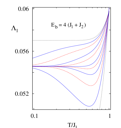
Figure 1: (Color online) Normalized spectral gaps $\Lambda_{1}\equiv e^{E_{b}/T}\,\lambda_{1}$ of the evolution operator for $L=20$ on approaching low-temperature regimes in sectors (a) and (b) of Table 2. From top to bottom, alternating solid and dashed lines stand for coupling ratios $r\equiv J_{2}/J_{1}=0.95,\,0.9,\,0.8,\,0.7,\,0.5,\,0.4,\,0.3,\,0.2,\,0.1$. Upper- and lowermost dotted curves denoting respectively the cases $r=1$ [ sector (c) ] and $r=0$, are shown for comparison. Details of that latter standard case are displayed in Fig. 2(a).

$r=J_{2}/J_{1}$ in sectors (a), (b), and (c) in a chain of 20 sites. As temperature decreases, the saturated behavior of most of the $r$ values considered clearly signals the emergence of the expected Arrhenius regime. Note that even a slight deviation from the conjectured barriers would result in strong departures from this behavior. Also, the saturation values of $\Lambda_{1}$, i.e. the amplitudes involved in Eq. (18), come out to be $r$- independent so long as $r\neq 0,1$. Apart from finite-size corrections (Fig. 2), this independence also holds for all other accessible lengths (a general feature applying also to other sectors of Table 2). However in approaching $r=0^{+}$ or $1^{-}$, where discontinuities already appear at the level of transition rates (see Table 1), the Arrhenius trend is only incipient and in some limiting cases it remains beyond our reach.

When it comes to dynamic exponents ($z$), in the main panels of Fig. 2 we show the finite-size behavior of these normalized gaps comparing the case of $J_{2}=0$ with others in sectors (a) and (b).

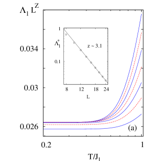
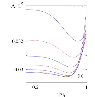
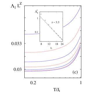
Figure 2: (Color online) Finite-size scaling of normalized gaps $e^{4\,(K_{1}+K_{2})}\,\lambda_{1}$ for (a) $r=0$ (usual ferromagnetic dynamics), (b) $r=0.3$, and (c) $r=0.7$. Solid and dashed lines show alternately the cases of $L=12,14,16,18,20,22,24$. In (a) sizes increase in upward order, while in (b) and (c) they do so from top to bottom. The data collapse of larger sizes was attained using dynamic exponents read off from the slope of the insets. These latter estimate the finite-size decay of spectral gaps close to $T\to 0^{+}$ [ (Eq. (18) ]. In that limit, the decay of (b) (not shown) is indistinguishable from that of (c) due to the common saturation trends of Fig. 1. For displaying convenience vertical scales of main panels were normalized by a factor $24^{z}$.

Clearly, the data collapse onto larger sizes is better for the standard dynamics, although in all cases the dynamic exponents producing these scaling plots are close to $z=3$ (check later on the extrapolations given in Sec. IV D). In turn, their values were estimated from the slopes fitting the finite-size decay of $\Lambda_{1}$ at the saturation limit (insets of Fig. 2), this being almost identical in (a) and (b) as it is evidenced in Fig. 1.

The above observations can also be extended to Fig. (3), where the normalized gaps of sectors (c) and (d) are exhibited. In parallel with the difficulties occurring in Fig. (1) as $r\to 1^{-}$, here these also appear in approaching the

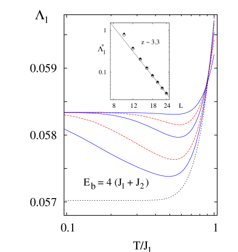
Figure 3: (Color online) Normalized gaps $e^{E_{b}/T}\,\lambda_{1}$ for $L=20$ within regime (d) of Table 2. From top to bottom solid and dashed lines refer in turn to coupling ratios $r=1.5,\,1.3,\,1.2,\,1.1,\,1.05$. For comparison, also the case $r=1$ [ regime (c) ] is shown by the dotted line. The inset estimates the typical finite-size decay of these gaps in the low-temperature limit [ (Eq. (18) ]. Filled triangles are representative of $r>1$ in sector (d), while open circles stand for $r=1$. However, see extrapolations of Sec. IV D.

limit of $r=1^{+}$. But otherwise, as before, the Arrhenius regime can be reached already within our low temperature ranges. In that respect, the inset shows that the common finite-size decay of $\Lambda_{1}^{\!{}^{*}}$ in sector (d) closely follows that of (c) ($r=1$), both regimes being characterized by a slope (dynamic exponent) very close to that obtained for sectors (a) and (b). Thus, an asymptotic scaling regime similar to the standard one of $J_{2}=0$ might be expected in these first four cases (despite the different proliferation rates of their corresponding M- states). But for the moment we defer that discussion to Sec. IV D.

IV.2 $J_{1}<0,\;J_{2}>0$

Next we turn to regime (e) where, as referred to in Sec. III, the dynamics follows a rather different decay pattern into AF states on time scales $\propto e^{4K_{2}}$. As temperature is lowered, the saturation trends observed in Fig. 4(a) already disclose the emergence of these Arrhenius factors for several $r$- coupling ratios. As in the previous subsection, the agreement with the former is very precise given the persistence of the $\Lambda_{1}$ plateaus. Also, the amplitudes concerning Eq. (18) here turn out to be $r$- independent although, likewise with what occurs in Fig. (1), as $|r|$ decreases the Arrhenius regime barely shows up for $T/|J_{1}|\gtrsim 0.1$. On the other hand, the trend of decreasing minima approaching the standard non-metastable gaps of $J_{2}=0$ is disrupted in the low temperature limit. As discussed below, this already signals an abrupt crossover of scaling regimes.

Note that regardless of how small $r$ might be, the metastability of this sector does not disappear so long as $J_{2}>0$. Thus, in the limit of $r=0^{-}$ this poses a situation reminiscent to that mentioned in Sec. I for the 1D Glauber dynamics under weak competing interactions. Irrespective of the weakness of the frustration, in the limit of $T\to 0^{+}$ metastability takes over and changes the dynamic exponents of that non-conserving dynamics from diffusive ($z=2$) to almost ballistic ($z\sim 1$) Grynberg . In that regard, here the analogy goes deeper as a similar discontinuity in scaling regimes also appears in this (non-frustrated) sector. This is exemplified for $r=-0.5$ in the scaling plot of Fig. 4(b) where the data collapse towards larger sizes is attained on choosing a dynamic exponent $z\sim 1.4$, in turn read off from the slope of the inset. As in Sec. IV A, this latter depicts the finite-size behavior of normalized gaps within the common saturation regime of Fig. 4(a), thus showing a $\Lambda_{1}^{\!{}^{*}}$- decay which presumably is also representative of all $r\in$ (e). Let us anticipate that the dynamic exponent arising from the finite-size extrapolations of these data (see Sec. IV D) also tends to a nearly ballistic value, far apart from the standard diffusive case of $J_{1}<0$ ($z\sim 2$, see Fig. 5 below) as well as from the subdiffusive one with $J_{1}>0$ [ $z\sim 3.1$, Fig. 2(a) ].

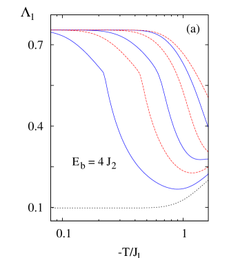
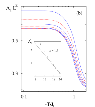
Figure 4: (Color online) (a) Normalized gaps $e^{E_{b}/T}\,\lambda_{1}$ in regime (e) of Table 2 using $L=20$ . From left to right solid and dashed lines denote in turn the cases of $-r=0.1,\,0.2,\,0.3,\,0.5,\,0.8,1.5$. Cusps stem from level crossings in the spectrum of the evolution operator. The dotted line shows for comparison the standard case of $r=0$ with $J_{1}<0$.  (b) Finite-size scaling of normalized gaps for $r=-0.5$ upon identifying $z$ with the slope of the inset. Alternating solid and dashed lines in downward direction indicate sizes $L=12,14,16,18,20,22,24$. For displaying purposes the vertical scale was normalized by a factor $24^{z}$. The inset estimates the typical finite-size decay of these gaps within sector (e) in the limit of $T\to 0^{+}$. See however extrapolations of Sec. IV D.

IV.3 $J_{1},\,J_{2}<0$

Before moving on to other sectors of Table 2, first we consider the non-metastable regime mentioned by the end of Sec. III, namely the situation of $J_{1}<0$ with $0\leq r<1/2$. As in sector (e), here the phase ordering is still AF. In Fig. 5(a) we display the plain spectral gaps for several coupling ratios in this region [ no need of normalization as in Eq. (18) ].

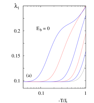
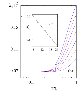
Figure 5: (Color online) (a) First excitation level of the evolution operator for $J_{1},\,J_{2}<0$ and $L=20$ in the non-metastable region $0\leq r<1/2$. From left to right solid and dashed lines refer alternately to coupling ratios $r=0.45,\,0.4,\,0.3,\,0.2,\,0.1$. The case $r=0$ is also shown for comparison (doted line).  (b) Scaling plot of these levels for $r=0.3$ and $L=24,22,20,18,16,14,12$ (solid and dashed lines from top to bottom) using $z=2$. For convenience the vertical scale was normalized by a factor $24^{2}$. The slope of the inset corroborates a common diffusive decay in the low-temperature limit of all ratios considered in panel (a).

Contrariwise to all other sectors, in this case the relaxation times ($1/\lambda_{1}$) of finite chains are kept bounded in the low-temperature limit, and so the Lanczos convergence is now faster. Unlike the Glauber case briefly touched upon in Sec. IV B, here the presence of frustration does not bring about changes in scaling regimes. Taking for instance $r=0.3$, this is checked in Fig. 5(b) where at low-temperatures all finite-size data can be made to collapse into a single curve by choosing the same diffusive exponent of the standard AF dynamics. In turn, the inset also corroborates this by estimating the slope with which these gaps decay with the system size as $T\to 0$. Since in that limit $\lambda_{1}$ becomes $r$- independent (just as do the amplitudes accompanying the Arrhenius factors in the above subsections), clearly this scaling behavior persists through the entire non-metastable region.

Turning to sectors (f) and (g), there are various thermal barriers affecting the decay of their respective M- structures, namely (in increasing order) $2Q,\,-4K_{2}\,$ for $r\in$ (f), and $2P,\,-4K_{2},\,2Q\,$ for $r\in$ (g). Among these barriers, it turns out that actually the largest one of each sector is comprised in the normalized gaps exhibited in Fig. 6. As before, the precision of the corresponding Arrhenius

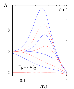
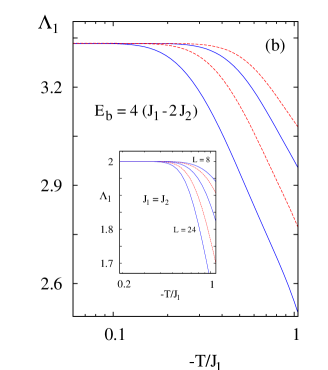
Figure 6: (Color online) Normalized gaps $e^{E_{b}/T}\,\lambda_{1}$ for $L=20$ in sectors (f) and (g) of Table 2 [ panels (a) and (b) respectively, exhibiting results of several coupling ratios ]. From top to bottom solid and dashed lines stand in turn for (a), $r=0.7,\,0.712,\,0.725,\,0.75,\,0.8,\,0.9,\,0.95,\,1$, and (b), $r=1.5,\,1.4,\,1.3,\,1.2$. The inset shows the case of $r=1$ for which these gaps become size-independent in nearing the Arrhenius regime. Here, lengths $L=24,20,16,12,8$ (in upward direction) match the four-fold periodicity of the ground state alluded to in the text.

factors is reflected in the clear saturation behavior obtained in the low-temperature regime. However just as in Sec. IV A, in approaching $r=1^{-},1^{+}$ or $1/2^{+}$ [ where the trend of increasing maxima continues for heights larger than the range of Fig. 6(a) ], the discontinuities arising in transition rates carry that saturation limit beyond our reach. But surprisingly, as is shown by the inset of Fig. 6(b), for $r=1$ that limit becomes size- independent. This suggests an exponentially fast relaxation even in the thermodynamic limit, though as $T\to 0^{+}$ the time scales involved get arbitrarily large, i.e. $\tau\simeq\frac{1}{2}\,e^{-4K_{2}}$.

In considering the finite-size behavior of $\Lambda_{1}^{\!{}^{*}}(L)$ for other coupling ratios in sectors (f) and (g), note that there the four-fold periodicity of the ground state $\,\cdots\bullet\bullet\circ\circ\cdots$ mentioned by the beginning of Sec. II leaves us with few sizes to draw conclusions about dynamic exponents. However, it is worth mentioning that the rather small logarithmic slopes resulting from the gaps of $L=16,20$ and 24 (namely, $0.18$ and 0.16), are consistent with the size- independent gaps obtained for $r=1$.

Sector (h).–  As before, there are several thermal barriers affecting the M- states of this sector ($-4K_{2},4K_{1},2P,2Q$), though now the largest one ($2Q$) ends up imposing even more severe restrictions on the Lanczos procedure as temperature is lowered. In fact, for $L>16$ the relenting convergence pace precluded us to obtain further results within the Arrhenius regime. In part, this also stems from level crossings in the spectrum of the evolution operator, on the other hand responsible for the pointed cusps observed in Fig. 7. There, we just content with evidencing the presence of a common activation factor characterizing the decay towards either the ferromagnetic or four-fold ground state ($-1/2<r<0$, or $r<-1/2$ respectively).

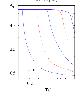
Figure 7: (Color online) Normalized gaps $e^{E_{b}/T}\,\lambda_{1}$ in regime (h) of Table 2, using $L=16$ for $-r=0.1,\,0.2,\,0.3,\,0.4,\,0.55,\,1.5$ (solid and dashed lines from left to right).

IV.4 Extrapolations

Armed with the finite-size estimations of the normalized gaps evaluated in Secs. IV A and IV B, next we turn to the issue of going a step further than the scaling plots considered so far. In that respect, an improved estimation of dynamic exponents can be made by introducing the sequence of approximants or effective exponents

$$Z_{L}=\frac{\ln[\,\Lambda_{1}^{\!{}^{*}}(L)/\Lambda_{1}^{\!{}^{*}}(L\!-\!2)\,]}{\ln[\,(L\!-\!2)/L\,]}\,,$$ (19)

each of which simply derives a measure of $z$ from the gaps of successive chain lengths. Similarly, it is worth introducing a sequence of approximants to the amplitudes involved in Eq. (18), as their common saturation values strongly suggest that these quantities are robust within each coupling sector of Table 2. Thus, concurrently with Eq. (19) we shall also consider the accompanying set of effective amplitudes $A_{L}$ given by

$$\ln A_{L}=\frac{\ln\Lambda_{1}^{\!{}^{*}}(L)\,\ln(L\!-\!2)\,-\,\ln\Lambda_{1}^{\!{}^{*}}(L\!-\!2)\,\ln(L)}{\ln[\,(L\!-\!2)/L\,]}\,.$$ (20)

In general, the elements $x_{L}$ of a finite-size sequence obtained close to a critical point (here $T=0^{+}$), are assumed to converge logarithmically Henkel ; Guttmann as $x_{L}=x+\sum_{j}\alpha_{j}L^{-a_{j}}$, with $\alpha$- constants and $a$- exponents such that $0<a_{j}<a_{j+1},\;\forall\,j$. To minimize the number of fitting parameters here we keep only the leading-order term of that expansion which just leave us with a nonlinear least-squares fit of three quantities. The results of those regressions are depicted in Fig. 8 which summarizes the trends of sequences (19) and (20) across sectors (a) to (e), together with those found in the non-metastable region. Specifically, the extrapolated exponents and amplitudes of each case turn out to be

$$z,\;\ln A\simeq\begin{cases}\,3.09(5),\;\;6.3(1)\,,\;\;\;\,{\rm for}\,\,J_{1},J_{2}\in\,{\rm{\it(a)}\,\,or\,\,{\it(b)}}\,,\vspace{0.1cm}\cr\,3.13(3),\;\;6.2(1)\,,\;\;\;\,{\rm for}\,\,J_{1},J_{2}\in\,{\rm{\it(c)}\,\,or\,\,{\it(d)}}\,,\vspace{0.1cm}\cr\,1.11(3),\;\;2.74(9)\,,\;\;{\rm for}\,\,J_{1},J_{2}\in\,{\rm{\it(e)}}\,,\vspace{0.1cm}\cr\,1.996(2),\,3.67(1),\,\,\;{\rm for}\,\,0\leq r<1/2,\;J_{1}<0\,.\end{cases}$$ (21)

The pace of convergence of effective exponents in sectors (a) and (b) comes out slightly slower than that arising in (c) and (d) ($a\sim 1.97$ and 2.07 respectively), though in the case of effective amplitudes that pace is inverted ($a\sim 1.76$ and 1.58). In sector (e) the convergence is still a bit slower [ $a\sim 1.75$ in Fig. 8(a) and $\sim 1.4$ in Fig. 8(b) ], but as anticipated in Sec. IV B the extrapolated dynamic exponent is close to that resulting from the 1D Glauber dynamics under weak competing interactions Grynberg . Thus, both scenarios are characterized by a discontinuous crossover from a non-metastable diffusive regime to a metastable one with nearly ballistic exponents. In the former case ($E_{b}=0$) the convergence is somewhat faster ($a\sim 2.2$ for exponents, and $\sim 1.97$ for

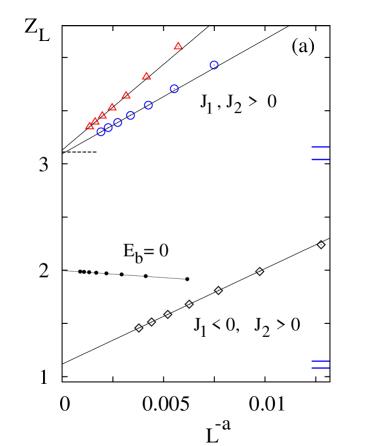
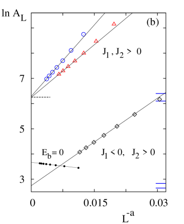
Figure 8: (Color online) Extrapolations of effective dynamic exponents (a), and amplitudes (b) defined in Eqs. (19) and (20). Data of regimes (a) and (b) (listed in Table 2), are represented by circles, regimes (c) and (d) by triangles, and regime (e) by rhomboids. Rightmost horizontal lines depict the confidence intervals arising from non-linear fittings in those regimes (see text for details). Leftmost dashed lines indicate the limiting values of the rapidly converging approximants for the usual case of $J_{2}=0,\,J_{1}>0$. Small dots stand for results in the non-metastable sector $0\leq r<1/2$ with $J_{1}<0$.

amplitudes) and the estimated errors become smaller than 0.3%. By contrast, in sectors (a) to (d) the errors are such that the resulting confidence intervals superpose each other [ see Eq. (21) ], though this is also due to the slight differences between the extrapolated values obtained in those sectors. Since in practice it is never really clear whether the assumed asymptotic behavior is sufficiently well realized by the data available Henkel , those differences might well be ascribed to our finite-size limitations. In that sense, the merging of confidence intervals [ rightmost center of panels 8(a) and 8(b) ] suggests a common characterization of these four sectors (as anticipated by the end of Sec. IV A), within an error margin of less than $\sim 5\%$. On this particular, it is also worth pointing out that for the standard ferromagnetic case of $J_{2}=0$ the differences between our higher approximants, namely $Z_{24}-Z_{22}$ and $\ln(A_{24}/A_{22})$, are both less than 0.02% [ also see Fig. 2(a) ]. The corresponding sequences approach swiftly towards $z\simeq\!3.11$  (thus suggesting a slightly slower kinetics than the Lifschitz-Slyozov type Huse  ), and $\ln A\simeq 6.25$, both values being consistent with Eq. (21) and included within the merged intervals of Fig. 8.

Finally, we should add that the seemingly fast convergence of approximants (19) and (20) in Fig. 8 only occurs within a small region of our scaled sizes ($1/L^{a}$,  $a>1$). This is due to the big $\alpha$- slopes stemming from our nonlinear least-squares fits, so that the measure of successive errors is actually $\alpha/L^{a}$. Nonetheless, the larger extrapolated errors of Eq. (21) resulted in less than 4%.

V Concluding remarks

To summarize, we have studied a 1D Kawasaki dynamics considering up to second neighbor interactions thus uncovering a range of metastable situations [ sectors (a) to (h) specified in Table 2 ]. Following the thread of arguments given in the Glauber counterpart Grynberg , we have constructed a quantum spin analogy whose ‘Hamiltonian’ [ Eqs. (12), (17a), and (17b) ] played the role of the evolution operator of these processes in the kink representation (see Table 1). The relaxation times of these former were then evaluated numerically in finite chains by analyzing the spectral gaps associated with those Hamiltonians using standard recursive methods Lanczos . We focused attention on the low but nonzero-temperature regimes where magnetic domains tend to coarsen and relaxation times can grow arbitrarily large  -even for finite chains-  due to the activation barriers discussed through Secs. III and IV. The usual finite-size scaling hypothesis (1) was then ‘normalized’ as in Eq. (18) so as to actually scale the spectral gaps of each sector within their corresponding Arrhenius regimes.

At time scales of order $e^{\,4\,(K_{1}+K_{2})}$ the decay patterns of sectors (a) to (d) were argued to be those of the standard ferromagnetic case details , although the proliferation of metastable states in sectors (b) and (c) turns out to be smaller. However, those differences appear to have no effect on the dynamic exponents, at least within the confidence intervals estimated in the extrapolations of Sec. IV D [ Eq. (21) and Fig. 8(a) ]. By contrast, those extrapolations yielded nearly ballistic values for the exponents of sector (e), on the other hand conjectured to decay through times $\propto e^{\,4K_{2}}$ in a rather different form. Note here then the abrupt crossover of scaling regimes in passing from sector (d) to (e). Also, in moving from this latter to the non-metastable region $0\leq J_{2}/J_{1}<1/2$ with $J_{1}<0$, another discontinuous change of dynamic exponents occurs. In the absence of activation barriers now these former become diffusive [ Figs. 5(b) and 8(a) ] whilst the relaxation time of finite systems remains bounded even at $T=0$. This situation is highly reminiscent of that of the Glauber dynamics studied in Ref. Grynberg where the sudden emergence of metastable states under a small $J_{2}<0$ also changes these exponents from diffusive to nearly ballistic.

When it comes to sectors (f) and (g) the four-fold periodicity of the ground state mentioned in Sec. II left us with few sizes to consider in Eq. (18), thus restricting our ability to extrapolate dynamic exponents. However for $J_{1}=J_{2}<0$, just where the activation barriers of these sectors coincide (see Table 2), surprisingly the normalized gaps become independent of the system size in the Arrhenius regime [ inset of Fig. 6(b) ]. Clearly, this suggests an exponential relaxation to equilibrium through time scales $\propto e^{-4K_{2}}$ that would persist up to the thermodynamic limit. In turn, this would be consistent with the small exponents preliminarily obtained for other coupling ratios in these sectors, but that is an issue requiring further investigation. Similarly, the study of sector (h) remains quite open given the convergence difficulties encountered in larger chains as temperature is decreased. Nonetheless, all sectors indicate that the amplitudes involved in Eq. (18) possibly stand for piecewise- universal quantities. Except at $J_{2}/J_{1}=0,1/2,1$, where the original transition rates get discontinuous in the limit of $T\to 0^{+}$, this is evidenced by the common saturation values of normalized gaps observed throughout Figs. 1, 3, 4(a), 5(a), 6(a), 6(b), and 7. As with dynamic exponents, those values were extrapolated to their thermodynamic limit in sectors (a) to (e) as well as in the non-metastable region [ Eq. (21) and Fig. 8(b) ].

In common to a variety of finite-size scaling studies (see e.g. Ref. Henkel and references therein), ultimately small sized systems have been analyzed. Often, as is the case here, the dimensionality of the operators involved (transfer matrices, Liouvillians, quantum Hamiltonians) grows exponentially with the system size thus severely limiting the manageable length scales, even for optimized algorithms. In an attempt to avoid those limitations we also considered the scaling of relaxation times in larger chains via Monte Carlo simulations. However, due to the Arrhenius barriers the difficulties introduced by small temperatures in such simulations are by far more restrictive than those associated to the system size (recall that $\tau\propto e^{E_{b}/T}L^{z}$). In fact, starting from a disordered phase and quenching down to $T/|J_{1}|$ within the range of $0.1-\,0.2$, it turned out that a significant fraction of the evolutions considered gets stuck in the typical metastable states of Table 2, even at large times.

Finally, and with regard to a possible extension of this study, it would be interesting to derive the activation barriers $E_{b}$ quoted in that latter Table directly from the evolution operator $\cal H$ constructed in Sec. II A. However irrespective of the sector considered, note that for $T\to 0^{+}$ the leading-order of its diagonal terms [ Eq. (12) ] is different from that of their non-diagonal counterparts [ Eqs. (17a) and(17b) ]. Thereby, the identification of an overall Arrhenius factor in the low-temperature limit of $\cal H$ is not evident in the kink representation. But in view of the universal amplitudes obtained above, one can further ask whether there might be a uniform spin rotation $R$ around a sector dependent axis such that $\!\!\underset{T\to 0^{+}}{\lim}R\,{\cal H}\,R^{-1}=e^{\,-\beta E_{b}}\;{\cal\hat{C}}$, for some sector-wise but constant operator $\cal\hat{C}$. That would not only single out activation barriers but would also allow computational access to the strict limit of $T\to 0^{+}$ via the low-lying eigenvalues of $\cal\hat{C}$. Further work along that line is under consideration.

Appendix A Proliferation of metastable states

As schematized in Table 2, these metastable (M) structures are characterized by the restrictions imposed on the number of consecutive kinks ($k$) and vacancies ($\rm v$) scattered throughout the chain. In turn, for each coupling sector these constraints affect the rate at which these configurations proliferate with the system size. In order to evaluate such specific rates, in what follows we will construct a set of recursive relations for the number $M_{L}$ of those states on chains of generic length $L$. To ease the analysis, open boundary conditions (OBC) will be assumed throughout. Below, we address each case in turn.

(a).–  Since for this sector $k=1$ and ${\rm v}\geq 1$, it is helpful to consider the relation between the quantities $F_{L}(1)$ and $F_{L}(0)$ defined as the number of M- configurations of length $L$ having respectively 1 or 0 as kink occupations on their first site. Clearly, under OBC these latter quantities must then be recursively related as

$$F_{L}(1)=F_{L-1}(0)\,,\;\;F_{L}(0)=F_{L-1}(0)+F_{L-1}(1)\,.$$ (22)

Therefore, either of these quantities as well as the total number $M_{L}=F_{L}(0)+F_{L}(1)$ of M- states follow a Fibonacci recursion $M_{L+2}=M_{L+1}+M_{L}$, from which an exponential growth $M_{L}\propto g^{L}$ with golden mean $g=(1+\sqrt{5})/2$ is obtained for large sizes (this growth also coincides with that of the ground state degeneracy at $-J_{2}/|J_{1}|=\frac{1}{2}$ Gori  ).

(b).–  In addition to the kink restrictions of the previous case, here there is also a ban on sequence parts of the form $...\,10101\,...$ as indicated in Table 2. To take into account that further constraint it is now convenient to introduce the number $G_{L}(n_{1},n_{2})$ of M- sequences of length $L$ having $n_{1}$ and $n_{2}$ as their first and second characters respectively ($n_{1},n_{2}=$ 0 or 1). Under OBC it is then a simple matter to check that these quantities must be related as

$$G_{L}(0,0) = G_{L-1}(0,0)+G_{L-2}(1,0)\,,$$ (23a)

$$G_{L}(0,1) = G_{L-1}(1,0)-G_{L-2}(0,1)\,,$$ (23b)

$$G_{L}(1,0) = G_{L-1}(0,0)+G_{L-1}(0,1)\,,$$ (23c)

while clearly $G_{L}(1,1)\equiv 0$. In Eq. (23b),  $G_{L-2}(0,1)$ cancels out just all extra sequences from $G_{L-1}(0,1)$ which would not form part of $G_{L}(0,1)$. Thereby, it can be readily verified that all $G$’s, along with the total number of M- states, i.e. $M_{L}=\sum_{n_{1},n_{2}}G_{L}(n_{1},n_{2})$, will then follow the recurrence

$$M_{L+5}=M_{L+4}+M_{L+2}+M_{L}\,.$$ (24)

The general solution of this latter Lando is associated to the roots of the polynomial $x^{5}-x^{4}-x^{2}-1$, thus for long chains, where the largest root dominates, the M- configurations of this sector finally turn out to grow as $\sim 1.5701^{L}$.

(c).–  Further to $k=1$, in this coupling sector every kink must appear separated by at least two vacancies, i.e. ${\rm v\geq 2}$, so now there are even more reductions in the number of M- states. On considering for instance the $F_{L}(0)$ and $F_{L}(1)$ quantities referred to in case (a), it is clear that under OBC here these should verify

$$F_{L}(0)=F_{L-1}(0)+F_{L-2}(1)\,,\;\;\;F_{L}(1)=F_{L-1}(0)\,,$$ (25)

from where the total number of M- configurations is obtained recursively as

$$M_{L+3}=M_{L+2}+M_{L}\,.$$ (26)

Thus, for $L\gg 1$ the largest root of the associated polynomial $x^{3}-x^{2}-1$ implies that $M_{L}\propto 1.4655^{L}$.

(d).–  In this case not only $\rm v\geq 2$ and $k=1$, but also there may be consecutive kinks now appearing in groups of $k>3$. To evaluate the proliferation of the corresponding M- states it is convenient to reintroduce here the $G_{L}(n_{1},n_{2})$ quantities referred to in case (b). For these latter, we readily obtain the recursive relations

$$G_{L}(0,0) = G_{L-1}(0,0)+G_{L-2}(1,0)+G_{L-2}(1,1)\,,$$

$$G_{L}(1,0) = G_{L-1}(0,0)\,,$$ (27)

$$G_{L}(1,1) = G_{L-1}(1,1)+G_{L-3}(1,0)\,,$$

(OBC throughout), evidently now with $G_{L}(0,1)\equiv 0$ as there can be no isolated vacancies. Thus, after a small amount of algebra it turns out that the total number of M- configurations as well as all $G^{\prime}s$ satisfy the recursive form

$$M_{L+6}=2\,M_{L+5}-M_{L+4}+M_{L+3}-M_{L+2}+M_{L}\,,$$ (28)

from where the golden mean is recovered in the largest root of the associated polynomial $x^{6}-2x^{5}+x^{4}-x^{3}+x^{2}-1$. Hence, analogously to sector (a), in the thermodynamic limit $M_{L}$ proliferates as $g^{L}$.

(e).–  As it was referred to in Table 2 for this coupling regime $k\geq 3$ and $\rm v\geq 2$. Thus, resorting back to the $G_{L}(n_{1},n_{2})$ quantities considered above we readily find that in this sector these must be related as

$$G_{L}(0,0) = G_{L-1}(0,0)+G_{L-2}(1,1)\,,$$ (29)

$$G_{L}(1,1) = G_{L-1}(1,1)+G_{L-3}(0,0)\,,$$

whereas $G_{L}(0,1)=G_{L}(1,0)=0$, as neither vacancies nor kinks may appear isolated in this case (OBC assumed). Thereby, it can be checked that the total number of M- states is given recursively by

$$M_{L+5}=2\,M_{L+4}-M_{L+3}+M_{L}\,.$$ (30)

From the largest root of the polynomial $x^{5}-2x^{4}+x^{3}-1$ linked to this recurrence, it then follows that for large sizes $M_{L}$ finally grows as $\sim 1.5289^{L}$.

(f).–  In this sector kinks and vacancy constraints are respectively specified by $k=1,2$, and $\rm v=1$. Therefore, in terms of the $G$-quantities introduced above this means that their recursion relations should now read

$$G_{L}(0,1) = G_{L-1}(1,0)+G_{L-1}(1,1)\,,$$

$$G_{L}(1,0) = G_{L-1}(0,1)\,,$$ (31)

$$G_{L}(1,1) = G_{L-1}(1,0)\,,$$

while clearly $G_{\!L}(0,0)\equiv 0$. Hence, after simple substitutions it is found that each of these $G$’s, and correspondingly the total number of M- states, all follow the recursive form

$$M_{L+3}=M_{L+1}+M_{L}\,,$$ (32)

which for large sizes is taken over by the largest root of the polynomial $x^{3}-x-1$. Thereby, it turns out that for this coupling regime $M_{L}$ grows only as fast as $\sim 1.3247^{L}$.

(g).–  Following Table 2, in this coupling regime $k=1,2$ (as before), but now $\rm v\geq 1$. In addition, there is also the constraint impeding the appearance of sequence parts of the form $...\,00100\,...$ Hence, assuming as usual OBC, the four $G$- quantities of this case must be linked recursively as

$$G_{L}(0,0) = G_{L-1}(0,0)+G_{L-1}(0,1)-G_{L-3}(0,0)\,,$$ (33a)

$$G_{L}(0,1) = G_{L-1}(1,0)+G_{L-1}(1,1)\,,$$ (33b)

$$G_{L}(1,0) = G_{L-1}(0,0)+G_{L-1}(0,1)\,,$$ (33c)

$$G_{L}(1,1) = G_{L-1}(1,0)\,.$$ (33d)

Due to the above restriction, and on par with case (b), here $G_{L-3}(0,0)$ appears subtracting unwanted sequences which otherwise would overestimate $G_{L}(0,0)$ in Eq. (33a). It is then a straightforward matter to verify that all of the above $G$’s (and therefore also $M_{L}$), ought to comply with the relation

$$M_{L+6}=M_{L+5}+M_{L+4}+M_{L+1}+M_{L}\,.$$ (34)

So, the characteristic polynomial associated to this latter recurrence is $x^{6}-x^{5}-x^{4}-x-1$, from where it follows that at large sizes $M_{L}$ should proliferate as $\sim 1.7437^{L}$.

(h).–  Finally, in this sector kinks and vacancy restrictions remain as in the previous case except that the ban on the sequences referred to above is now lifted. Thus, recursions (33) still hold provided Eq. (33a) is modified as

$$G_{L}(0,0)=G_{L-1}(0,0)+G_{L-1}(0,1)\,,$$ (35)

i.e. the cancellation of sequences contained in $G_{L-3}(0,0)$ is no longer required here. After that modification it can be readily checked that the recursions arising in this coupling regime are all of the form

$$M_{L+3}=M_{L+2}+M_{L+1}+M_{L}\,.$$ (36)

From the largest root of $x^{3}-x^{2}-x-1$, we thus find that in the limit of large $L$ here $M_{L}$ grows as $\sim 1.8392^{L}$.

References

- (1) For reviews, consult Kinetics of Phase Transitions, edited by S. Puri and V. Wadhawan (CRC Press, Boca Raton, FL, 2009); A. J. Bray, Adv. Phys. 43, 357 (1994); J. D. Gunton, M. San Miguel, and P. S. Sahni, in Phase Transitions and Critical Phenomena, edited by C. Domb and J. L. Lebowitz (Academic Press, London, 1983), Vol. 8.
- (2) S. Dattagupta and S. Puri, Dissipative Phenomena in Condensed Matter: Some Applications, (Springer, Berlin, 2004); A. Onuki, Phase Transition Dynamics, (Cambridge University Press, 2002).
- (3) K. Kawasaki, in Phase Transitions and Critical Phenomena, edited by C. Domb and M. S. Green (Academic Press, London, 1972), Vol. 2.
- (4) R. J. Glauber, J. Math. Phys. 4, 294 (1963); B. U. Felderhof, Rep. Math. Phys. 1, 215 (1971).
- (5) K. Kawasaki, Phys. Rev. 145, 224 (1966).
- (6) At a coarse grained or hydrodynamic level of description both dynamics pertain to the classification scheme of P. C. Hohenberg and B. Halperin, Rev. Mod. Phys. 49, 435 (1977).
- (7) P. L. Krapivsky, S. Redner, and E. Ben-Naim, A Kinetic View of Statistical Physics (Cambridge University Press, 2010), Chap. 8.
- (8) Nonequilibrium Statistical Mechanics in One Dimension, edited by V. Privman (Cambridge University Press, 1997).
- (9) L. Bogani, C. Sangregorio, R. Sessoli, and D. Gatteschi, Angew. Chem., Int. Ed. Engl. 44, 5817 (2005); K. Bernot et al., J. Am. Chem. Soc. 128, 7947 (2006); A. Caneschi et al., Europhys. Lett. 58, 771 (2002).
- (10) M. G. Pini and A. Rettori, Phys. Rev. B 76, 064407 (2007).
- (11) M. D. Grynberg, Phys. Rev. E 91, 032129 (2015).
- (12) S. Redner and P. L. Krapivsky, J. Phys. A 31, 9229 (1998).
- (13) S. J. Cornell, K. Kaski, and R. B. Stinchcombe, Phys. Rev. B 44, 12263 (1991); see also S. J. Cornell in Ref. Privman and references therein.
- (14) For details, consult Section 8.7 of Ref. Redner .
- (15) N. G. van Kampen, Stochastic Processes in Physics and Chemistry, 3rd ed. (North-Holland, Amsterdam, 2007), Chap. 5.
- (16) See e.g. K. Tanaka, T. Morita, and K. Hiroike, Prog. Theor. Phys. 77, 68 (1987); R. M. Hornreich, R. Liebmann, H. G. Schuster, and W. Selke, Z. Phys. B 35, 91 (1979); J. Stephenson, Phys. Rev. B 1, 4405 (1970); J. Marro and R. Dickman, Nonequilibirum Phase Transitions in Lattice Models, (Cambridge University Press, 1999), Section 8.4.
- (17) Consult for instance, M. Henkel, H. Hinrichsen, and S Lübeck, Non-Equilibrium Phase Transitions, Vol. 1, (Springer, Dordrecht, 2008), Appendix F.
- (18) See for example, G. H. Golub and C. F. van Loan, Matrix Computations, 3rd. ed. (Johns Hopkins University Press, Baltimore, 1996); G. Meurant, The Lanczos and Conjugate Gradient Algorithms, (SIAM, Philadelphia, 2006).
- (19) A. J. Guttmann, in Phase Transitions and Critical Phenomena, edited by C. Domb and J. L. Lebowitz (Academic Press, London, 1989), Vol. 13.
- (20) M. Suzuki and R. Kubo, J. Phys. Soc. Jpn. 24, 51 (1968).
- (21) However, for exact results at large times of the zero-temperature dynamics, see G. De Smedt, C. Godrèche, and J. M. Luck, Eur. Phys. J. 32, 215 (2003); V. Privman, Phys. Rev. Lett. 69, 3686 (1992).
- (22) For these times are associated with the smallest activation barrier of this sector. Otherwise, the lead is taken by the first pairing process of Table 1, but its effects are inconsequential on times .
- (23) This just assumes the existence of at least one domain with an odd number of kinks in the metastable configurations.
- (24) For finite magnetizations the number of separating vacancies may be larger. Besides, three and four consecutive kinks may also appear, but here we just focus on the case of .
- (25) D. Huse, Phys. Rev. B 34, 7845 (1986); I. Lifschitz and V. Slyozov, J. Chem. Solids 19, 35 (1961).
- (26) G. Gori and A. Trombettoni, J. Stat. Mech. P10021 (2011).
- (27) S. K. Lando, Lectures on Generating Functions, Student Mathematical Library, Vol. 23, Chap. 2 (American Mathematical Society, Providence, 2003).