Interferometric Phase Estimation Though Quantum Filtering in Coherent States

Abstract

We derive the form of the quantum filter equation describing the continuous observation of the phase of a quantum system in an arm of an interferometer via non-demolition measurements when the statistics of an input field used for the indirect measurement are in a general coherent state. Both quadrature homodyne detection and photon-counting dection schemes are covered, and we solve the linearized filter for a specific application.

I Introduction

There has been a steady interest in the problem of “collapse of the wavefunction” amongst quantum physicists, particularly in relation to foundational issues. The dichotomy usually presented is between the unitary evolution under the Schrödinger equation and the discontinuous change when a measurement is made. Clearly the collapse of the wavefunction is a form of conditioning the quantum state made by an instantaneous measurement. However, conditional probabilities are well known classically and have no such interpretational issues. Furthermore, the process of extraction of information from a classical system and the resulting conditioning of the state is well studied from the point of view of stochastic estimation. For continual measurements, there are standard results on nonlinear filtering, see DavisMarcus ; Kush79 ; Kush80 ; Zak69 . What is not often appreciated in the theoretical physics community is that the analogue problem was formulated by Belavkin Bel80 ; Bel92a where a quantum theory of filtering based on non-demolition measurements of an output field is established: see also BouGutMaa04 -GJNC_PRA12 . Specifically, we must measure a particular feature of the field, for instance a field quadrature or the count of the field quanta, and this determines a self-commuting, therefore essentially classical, stochastic process. The resulting equations have structural similarities with the classical analogues. They are also formally identical with the equations arising in quantum trajectory theory Carmichael93 however the stochastic master equations play different roles: in quantum filtering they describe the conditioned evolution of the state while in quantum trajectories they are a means of simulating a master equation.

There has been recent interest amongst the physics community in quantum filtering as an applied technique in quantum feedback and control AASDM02 - WM93 . An additional driver is the desire to go beyond the situation of a vacuum field and derive the filter for other physically important states such as thermal, squeezed, single photon states, etc. In a previous publication G_scat_PRA15 we derived a quantum Markovian model for an opto-mechanical system consisting of a quantum mechanical mirror interacting with quantum optical input fields via radiation pressure, and in particular were able to construct the quantum filter for the position of the mirror based on the continual monitoring of scattered photons. To obtain a non-trivial result, we had to place the input fields in a coherent state of non-zero intensity and rely on the filtering theory for coherent state inputs GK_COSA10 . In this note we wish to treat the problem of constructing the filter for non-demolition quadrature and photon-counting measurements of the output of a Mach-Zehnder interferometer with the purpose of estimating the phase difference between the two arms of the interferometer: see Figure 1.

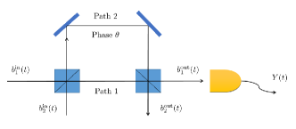
Figure 1: The model is fully quantum: we have a Mach-Zehnder interferometer in which there is a quantum mechanical phase associated with one of the arms (this may be due to one or more of the mirrors being an opto-mechanical system); the input fields are modelled a quantum input processes on the appropriate Boson Fock space (see Section II).

Here the phase is treated as a quantum mechanical object, so the problem is genuinely one of estimating the quantum state of the interferometer phase variable. As the interaction of the photons with the interferometer is purely scattering (so no emission or absorption) we must take one of input fields to be in a coherent state with intensity function $\beta$. The model may be thought of as the continuous variable analogue of the discrete model examined recently by Harrell in Harrell : indeed, it is reasonable to expect that the continuous time limit of this model leads to the results presented here by the time of arguments presented in G_Sob_2004 .

The paper is organized as follows. In Section II we describe the model of a Mach-Zehnder interferometer with appropriate continuous-variable quantum inputs. A fully quantum stochastic model of the interferometer phase observable and the photon fields is presented in terms of quantum stochastic calculus HP -GC85 . In Section III we describe the basic estimation problem and state the main result which is the form of the filters in the language of stochastic estimation: these may then be rewritten in terms of stochastic master equations, and we give the equivalent form for homodyning. In Section IV we derive the filters using the characteristic function approach. Finally in Section V we solve the filter in a linearized regime - equivalent to a quantum Kalman-Bucy filter and discuss the physical properties of the system including the “collapse of the wave-function”.

II The Experimental Set Up

We consider an interferometer as shown in Figure 1 where two continuous wave optical inputs $b_{1}^{\text{in}}$ and $b_{2}^{\text{in}}$ are mixed in a 50-50 beam splitter and then recombined in a second 50-50 beam splitter. The second path in the interferometer has a phase $\theta$ relative to the first path. We treat $\theta$ as a quantum mechanical observable and we aim to estimate the corresponding state by measuring one of the output fields. In this paper we will consider a homodyne scheme where we measure the quadrature associated with the output $b_{1}^{\text{out}}$. The problem would of course be trivial if both inputs where in the vacuum state, so we assume that one on the inputs, $b_{1}^{\text{in}}$ is in a coherent state while the other is in the vacuum.

The scattering matrix $S$ relating the inputs processes to outputs is given by the product $S=TPT$ where $T=\frac{1}{\sqrt{2}}\left[\begin{array}[]{cc}1&i\\ i&1\end{array}\right]$ and $P=\left[\begin{array}[]{cc}1&0\\ 0&-e^{i\theta}\end{array}\right]$ are the beam splitter matrix and interferometer path transfer matrix respectively. That is

$$S = \left[\begin{array}[]{cc}S_{11}&S_{12}\\ S_{21}&S_{22}\end{array}\right]$$ (3)

$$\equiv \frac{1}{2}\left[\begin{array}[]{cc}1+e^{i\theta}&i\left(1-e^{i\theta}\right)\\ i\left(1-e^{i\theta}\right)&-\left(1+e^{i\theta}\right)\end{array}\right].$$ (6)

Note that the entries $S_{jk}$ depend on the observable $\theta$ and are therefore operators on the associated Hilbert space $\mathfrak{h}$. We may additionally have a Hamiltonian $H$ leading to a non-trivial evolution of the observable $\theta$.

II.1 Fully Quantum Model

The inputs satisfy the singular commutation relations

$$\left[b_{j}^{\text{in}}\left(t\right),b_{k}^{\text{in*}}\left(s\right)\right]=\delta_{jk}\delta\left(t-s\right),$$

and in the following we shall work with the processes

$$B_{k}\left(t\right) = \int_{0}^{t}b_{k}^{\text{in}}\left(s\right)ds,$$

$$B_{k}\left(t\right)^{\ast} = \int_{0}^{t}b_{k}^{\text{in*}}\left(s\right)ds,$$

$$\Lambda_{jk}\left(t\right) = \int_{0}^{t}b_{j}^{\text{in*}}\left(s\right)b_{k}^{\text{in}}\left(s\right)ds,$$

which correspond to well defined operators on a Fock space $\mathfrak{F}$. The Hudson-Parthasarathy theory of quantum stochastic calculus HP gives an analogue of the Itō calculus for integrals with respect to these processes. We note the Itō table

$$dB_{j}dB_{k}^{\ast} = \delta_{jk}dt,$$

$$dB_{j}d\Lambda_{kl} = \delta_{jk}dB_{l},$$

$$d\Lambda_{jk}dB_{l}^{\ast} = \delta_{kl}dB_{j}^{\ast},$$

$$d\Lambda_{jk}d\Lambda_{lm} = \delta_{kl}d\Lambda_{jm},$$ (7)

with other products of differentials vanishing.

The general class of unitaries processes on $\mathfrak{h}\otimes\mathfrak{F}$ driven by these fundamental processes is given in HP involves coefficients $\left(S,L,H\right)$ corresponding to the scattering $S$, the coupling $L$ and the Hamiltonian $H$ for the non-field component. In our case their is no photo-emissive coupling of input fields with the interferometer, so we set $L=0$. The most general form then reduces to

$$dU_{t}=\left\{\sum_{j,k}\left(S_{jk}-\delta_{jk}\right)\otimes d\Lambda_{jk}\left(t\right)-iH\otimes dt\right\}U_{t},$$

with $S=\left[S_{jk}\right]$ unitary, that is

$$\sum_{k}S_{ki}^{\ast}S_{kj}=\delta_{ij}I_{\mathfrak{h}}=\sum_{k}S_{ik}S_{jk}^{\ast}.$$ (8)

II.2 Internal Dynamics of the Interferometer

For $X$ an arbitrary operator on the Hilbert space $\mathfrak{h}$ of the interferometer, its Heisenberg evolution is given by

$$j_{t}\left(X\right)=U_{t}^{\ast}\left(X\otimes I_{\mathfrak{F}}\right)U_{t}$$

and from the quantum Itō calculus we find Langevin equation

$$dj_{t}\left(X\right) = \sum_{i,j,k}j_{t}\left(S_{ki}^{\ast}XS_{kj}-\delta_{ij}X\right)\otimes d\Lambda_{ij}\left(t\right)$$

$$-ij_{t}\left(\left[X,H\right]\right)\otimes dt.$$

For the specific case of the scattering matrix (6) we find

$$dj_{t}\left(X\right)=-ij_{t}\left(\left[X,H\right]\right)\otimes dt$$

$$+\frac{1}{2}j_{t}\left(e^{-i\theta}Xe^{i\theta}-X\right)\otimes\left(d\Lambda_{11}-id\Lambda_{12}+id\Lambda_{21}+d\Lambda_{22}\right).$$

(9)

II.3 Input-Output Relations

The output fields $B_{j}^{\text{out}}\left(t\right)$ are defined by

$$B_{j}^{\text{out}}\left(t\right)\triangleq U_{t}^{\ast}\left(I_{\mathfrak{h}}\otimes B_{j}^{\text{in}}\left(t\right)\right)U_{t}$$

and again using the quantum Itō calculus we find

$$dB_{j}^{\text{out}}\left(t\right)=\sum_{k}j_{t}\left(S_{jk}\right)\otimes dB_{k}^{\text{in}}\left(t\right).$$

II.4 Homodyne Detection

Our objective is to estimate the state of the interferometer at time $t$ based on the observations of the output quadrature $Y$ of the first output up to time $t$. Here we have

$$Y\left(t\right) = B_{1}^{\text{out}}\left(t\right)+B_{1}^{\text{out}}\left(t\right)^{\ast}$$

$$= U_{t}^{\ast}\left(I_{\mathfrak{h}}\otimes\left(B_{1}^{\text{in}}\left(t\right)+B_{1}^{\text{in}}\left(t\right)^{\ast}\right)\right)U_{t}.$$

We note that

$$dY\left(t\right)=\sum_{k}j_{t}\left(S_{1k}\right)\otimes dB_{k}^{\text{in}}\left(t\right)+H.c.$$ (10)

The process $Y=Y^{\ast}$ is self-nondemolition by which we mean that $\left[Y\left(t\right),Y\left(s\right)\right]=0$ for all times $t,s$. It furthermore satisfies the nondemolition property that $\left[j_{t}\left(X\right),Y\left(s\right)\right]=0$ for all $t\geq s$, so that we may estimate present or future values of the observable $X$ in the Heisenberg picture based on the observations up to and including present time. We note that

$$\left(dY\right)^{2}=dt,$$

which follows from the quantum Itō table (7) and the unitarity condition (8).

Clearly the process $Y$ contains information about the scattering coefficients, however, it would possess the statistics of a standard Wiener process if we took the input fields to be in the vacuum state. It is for this reason we take the first input field to be in a coherent state corresponding to an intensity $\beta=\beta\left(t\right)$. The joint state is denoted as $\mathbb{E}_{\beta}$ and is the product state of the initial state of the interferometer (which may be a guess!) and the Gaussian state of the fields corresponding to input 1 in the coherent state with intensity $\beta$ and input 2 in the vacuum. Specifically, the Weyl operators have expectation

$$\mathbb{E}_{\beta}\left[e^{\sum_{k}\int f_{k}\left(t\right)dB_{k}^{\text{in}}\left(t\right)^{\ast}-H.c.}\right]=e^{-\frac{1}{2}\sum_{k}\int|f_{k}\left(t\right)|^{2}dt}\\ \times e^{\int f_{1}\left(t\right)\beta\left(t\right)^{\ast}dt-\int f_{1}\left(t\right)^{\ast}\beta\left(t\right)dt},$$

and so

$$\mathbb{E}_{\beta}\left[dY\left(t\right)\right]=\mathbb{E}_{\beta}\left[j_{t}\left(S_{11}\right)\right]\beta\left(t\right)dt+\mathbb{E}_{\beta}\left[j_{t}\left(S_{11}^{\ast}\right)\right]\beta\left(t\right)^{\ast}dt$$

(11)

which is non-zero for $\beta\left(t\right)\neq 0$.

II.5 Photon Counting Detection

Alternatively we could count the number of photons at the first output channel. This time the measured process $Y$ is

$$Y\left(t\right)=U_{t}^{\ast}\left(I_{\mathfrak{h}}\otimes\Lambda_{11}^{\text{out}}\left(t\right)\right)U_{t}$$

and from the Itō calculus we obtain

$$dY\left(t\right) = \sum_{j,k}j_{t}\left(S_{1j}^{\ast}S_{1k}\right)\otimes d\Lambda_{jk}^{\text{in}}\left(t\right)$$ (12)

$$= j_{t}\left(\frac{1+\cos\theta}{2}\right)\otimes d\Lambda_{11}^{\text{in}}\left(t\right)$$

$$+j_{t}\left(\frac{\sin\theta}{2}\right)\otimes\left[d\Lambda_{12}^{\text{in}}\left(t\right)+d\Lambda_{21}^{\text{in}}\left(t\right)\right]$$

$$+j_{t}\left(\frac{1-\cos\theta}{2}\right)\otimes d\Lambda_{22}^{\text{in}}\left(t\right).$$

Here we note that

$$\left(dY\right)^{2}=j_{t}\left(\frac{1+\cos^{2}\theta}{2}\right)\otimes d\Lambda_{11}^{\text{in}}\left(t\right)+\cdots$$ (13)

where the omitted terms are proportional to the increments $d\Lambda_{12}^{\text{in}}\left(t\right),d\Lambda_{21}^{\text{in}}\left(t\right)$ and $d\Lambda_{22}^{\text{in}}\left(t\right)$ which average to zero of the state $\mathbb{E}_{\beta}$.

III Quantum Filtering

Our goal is to derive the optimal estimate $\pi_{t}\left(X\right)$ for an observable $j_{t}\left(X\right)$ for the state $\mathbb{E}_{\beta}$ given the observations of $Y$ up to time $t$. To this end we set $\mathfrak{Y}_{t]}$ to be the (von Neumann) algebra generated by the family $\left\{Y\left(s\right):0\geq s\leq t\right\}$. As $Y$ is self-non-demolition, we have that $\mathfrak{Y}_{t]}$ is a commutative algebra - so the recorded measurement can be treated as an essentially classical stochastic process as it should be. Every observable that commutes with $\mathfrak{Y}_{t]}$ will possess a well-defined joint (classical) statistical distribution with the measurements up to time $t$ and by the non-demolition property this includes $j_{t}\left(X\right)$. We therefore set

$$\pi_{t}\left(X\right)=\mathbb{E}_{\beta}\left[j_{t}\left(X\right)|\mathfrak{Y}_{t]}\right]$$

which is the conditional expectation of $j_{t}\left(X\right)$ onto $\mathfrak{Y}_{t]}$. The right hand side always exists since the algebra generated by $\mathfrak{Y}_{t]}$ and the additional element $j_{t}\left(X\right)$ is commutative and so we exploit the fact that in classical probability theory conditional expectations always exist. This classical expectation is then understood as being a function of the commuting set $\left\{Y\left(s\right):0\geq s\leq t\right\}$. It should be remembered that $\pi_{t}\left(X\right)$ can be defined in this way for arbitrary observable $X$ of the interferometer system, and these $X$’s generally do not commute, so the construction is genuinely quantum in that regard. Note that while $\pi_{t}\left(X_{1}X_{2}\right)$ is generally different from $\pi_{t}\left(X_{2}X_{1}\right)$, we will however have $\left[\pi_{t}\left(X_{1}\right),\pi_{t}\left(X_{2}\right)\right]=0$ as we have conditioned onto the commutative algebra of operators $\mathfrak{Y}_{t]}$. Finally we mention that this estimate is optimal in the least squares sense. That is,for $X$ self-adjoint, we have

$$\mathbb{E}_{\beta}\bigg{[}\left(j_{t}\left(X\right)-\pi_{t}\left(X\right)\right)^{2}\bigg{]}\leq\mathbb{E}_{\beta}\bigg{[}\left(j_{t}\left(X\right)-\hat{X}_{t}\right)^{2}\bigg{]}$$

for all $\hat{X}_{t}\in\mathfrak{Y}_{t]}$. In particular we have the “orthogonality” property

$$\mathbb{E}_{\beta}\bigg{[}\left(j_{t}\left(X\right)-\pi_{t}\left(X\right)\right)C\left(t\right)\bigg{]}=0$$

for every $C\left(t\right)\in\mathfrak{Y}_{t]}$.

III.1 The Filtering Equation

We will now state the main result. In both cases the filtering equation takes the form

$$d\pi_{t}\left(X\right) = \frac{1}{2}\pi_{t}\left(e^{-i\theta}Xe^{i\theta}-X\right)|\beta\left(t\right)|^{2}-i\pi_{t}(\left[X,H\right])dt$$ (14)

$$+\mathcal{H}_{t}\left(X\right)\,dI\left(t\right),$$

The terms $\mathcal{H}_{t}(X)$ and the process $I(t)$ are specific to the physical mode of detection and we give these explicitly for the scheme of homodyne (quadrature) measurement and the photon counting scheme below.

III.1.1 Quadrature Measurement

In this case we measure the quadrature of output field 1. here we find that

$$\mathcal{H}_{t}\left(X\right) = \frac{1}{2}\left[\pi_{t}\left(Xe^{i\theta}\right)-\pi_{t}\left(X\right)\pi_{t}\left(e^{i\theta}\right)\right]\beta\left(t\right)$$

$$+ \frac{1}{2}\left[\pi_{t}\left(e^{-i\theta}X\right)-\pi_{t}\left(e^{-i\theta}\right)\pi_{t}\left(X\right)\right]\beta\left(t\right)^{\ast}.$$

The innovations process $I$ is defined by

$$dI\left(t\right)=dY\left(t\right)-\left[\pi_{t}\left(S_{11}\right)\beta\left(t\right)+\pi_{t}\left(S_{11}^{\ast}\right)\beta\left(t\right)^{\ast}\right]dt,$$

(16)

and $I\left(0\right)=0$. Statistically it has the distribution of a standard Wiener process.

We see that $dI\left(t\right)$ is the difference between the actual observed increment $dY\left(t\right)$ and the expected increment $\left[\pi_{t}\left(S_{11}\right)\beta\left(t\right)+\pi_{t}\left(S_{11}^{\ast}\right)\beta\left(t\right)^{\ast}\right]dt$ based on the filter. In stochastic estimation problems $I(t)$ is referred to as the innovations process.

III.1.2 Photon Counting Measurement

If instead we count the photons coming out of output 1, we obtain

$$\mathcal{H}_{t}(X) = \frac{1}{1+\pi_{t}\left(\cos^{2}\theta\right)}$$ (17)

$$\times\Big{\{}\frac{1}{2}\pi_{t}\left(e^{-i\theta}Xe^{i\theta}+e^{-i\theta}X+Xe^{i\theta}-X\right)$$

$$\quad\quad\qquad-\pi_{t}\left(X\right)\pi_{t}\left(\cos\theta\right)\Big{\}}.$$

The innovations process is this time given by

$$dI\left(t\right)=dY\left(t\right)-\pi_{t}\left(\frac{1+\cos\theta}{2}\right)|\beta\left(t\right)|^{2}dt,$$ (18)

and $I\left(0\right)=0$. This time the innovations have the statistical distribution of a compensated Poisson process. Once again, $dI(t)$ is the difference between the observed measurement increment $dY(t)$ and the expected increment $\mathbb{E}_{\beta}[dY(t)]$.

III.1.3 Equivalent Stochastic Master Equation

We may alternatively use the dual form for the filter where we express everything in terms of the conditional state $\varrho_{t}$ of the interferometer system based on the measurements so that

$$\pi_{t}\left(X\right)=\text{tr}\left\{\varrho_{t}X\right\}.$$

In the quadrature case, the filter equation thereby translates into the equivalent stochastic master equation (SME) for $\varrho_{t}$

$$d\varrho_{t} = \frac{1}{2}\left(e^{i\theta}\varrho_{t}e^{-i\theta}-\varrho_{t}\right)|\beta\left(t\right)|^{2}dt+i\left[\varrho_{t},H\right]dt$$ (19)

$$+\frac{1}{2}\left(e^{i\theta}\varrho_{t}-\zeta_{t}\varrho_{t}\right)\beta\left(t\right)dI\left(t\right)$$

$$+\frac{1}{2}\left(\varrho_{t}e^{-i\theta}-\zeta_{t}^{\ast}\varrho_{t}\right)\beta\left(t\right)^{\ast}dI\left(t\right)$$

where

$$\zeta_{t}=\text{tr}\left\{\varrho_{t}e^{i\theta}\right\}.$$ (20)

The presence of the term (20) in the SME (19) means that the equation is nonlinear. This filter is diffusive since the innovations are a standard Wiener process. An SME formulation may likewise be given for the photon counting: this again will be nonlinear, but this time will be driven by a jump process corresponding to the observation of a photon arrival at the detector.

If we choose to ignore the measurement record - a nonselective measurement - then we obtain the following master equation for $\bar{\rho}_{t}=\mathbb{E}_{\beta}\left[\varrho_{t}\right]$:

$$\frac{d\bar{\rho}_{t}}{dt}=\frac{1}{2}\left(e^{i\theta}\bar{\rho}_{t}e^{-i\theta}-\bar{\rho}_{t}\right)|\beta\left(t\right)|^{2}+i\left[\bar{\rho}_{t},H\right].$$ (21)

In the language of quantum trajectories, the SME (19) is an “unravelling” of the master equation (21). The same master equation is unravelled by the photon counting SME.

IV Derivation of the filters

In this section we derive the form of the filters given in Section III. We will use a technique known as the characteristic function approach. This is a direct method for calculating the filtered estimate $\pi_{t}\left(X\right)$ is based on introducing a process $C\left(t\right)$ satisfying the QSDE

$$dC\left(t\right)=f\left(t\right)C\left(t\right)dY\left(t\right),$$ (22)

with initial condition $C\left(0\right)=I$. Here we assume that $f$ is integrable, but otherwise arbitrary. The technique is to make an ansatz of the form

$$d\pi_{t}\left(X\right)=\mathcal{F}_{t}\left(X\right)dt+\mathcal{H}_{t}\left(X\right)dY\left(t\right)$$ (23)

where we assume that the processes $\mathcal{F}_{t}\left(X\right)$ and $\mathcal{H}_{t}\left(X\right)$ are adapted and lie in $\mathfrak{Y}_{t]}$. These coefficients may be deduced from the identity

$$\mathbb{E}\left[\left(\pi_{t}\left(X\right)-j_{t}\left(X\right)\right)C\left(t\right)\right]=0$$

which is valid since $C\left(t\right)\in\mathfrak{Y}_{t]}$. We note that the Itō product rule implies $I+II+III=0$ where

$$I = \mathbb{E}\left[\left(d\pi_{t}\left(X\right)-dj_{t}\left(X\right)\right)C\left(t\right)\right],$$

$$II = \mathbb{E}\left[\left(\pi_{t}\left(X\right)-j_{t}\left(X\right)\right)dC\left(t\right)\right],$$

$$III = \mathbb{E}\left[\left(d\pi_{t}\left(X\right)-dj_{t}\left(X\right)\right)dC\left(t\right)\right].$$

IV.1 The Quadrature Filter

We now compute the filter when $Y$ is the measured quadrature of the first output channel.

IV.1.1 Term I

Here we have (omitting $t$-dependence for ease of notation)

$$I=\mathbb{E}_{\beta}\left[\mathcal{F}\left(X\right)C+\mathcal{H}\left(X\right)(j(S_{11})\beta+j(S_{11}^{\ast})\beta^{\ast})C\right]dt\\ -\frac{1}{2}\mathbb{E}_{\beta}\left[j\left(e^{-i\theta}Xe^{i\theta}-X\right)C\right]|\beta|^{2}dt+i\mathbb{E}_{\beta}\left[\left[X,H\right]C\right]dt$$

where we use the fact that

$$\mathbb{E}_{\beta}\left[d\Lambda_{11}\left(t\right)\right]=|\beta\left(t\right)|^{2}dt$$

while $\mathbb{E}_{\beta}\left[d\Lambda_{jk}\left(t\right)\right]=0$ otherwise.

IV.1.2 Term II

From (11) we obtain

$$II=f\,\mathbb{E}_{\beta}\left[\left(\pi\left(X\right)-j(X)\right)C\left(t\right)j(S_{11})\beta+j(S_{11}^{\ast})\beta^{\ast}\right]dt.$$

IV.1.3 Term III

We have

$$III=f\,\mathbb{E}_{\beta}\left[\mathcal{H}\left(X\right)C\right]dt\\ -f\,\frac{1}{2}\mathbb{E}_{\beta}\left[j\left(e^{-i\theta}Xe^{i\theta}-X\right)\left(j\left(S_{11}^{\ast}\right)-ij\left(S_{12}^{\ast}\right)\right)\beta^{\ast}C\right]dt$$

where we use the fact that $\left(dY\right)^{2}=dt$ and from (9) and (10)

$$dj\left(X\right)dY = \frac{1}{2}j_{t}\left(e^{-i\theta}Xe^{i\theta}-X\right)$$

$$\times\left(j\left(S_{11}^{\ast}\right)-ij\left(S_{12}^{\ast}\right)\right)dB_{1}^{\ast}+\cdots$$

where the omitted terms average to zero. Note that we used the identities $d\Lambda_{11}dB_{1}^{\ast}=d\Lambda_{12}dB_{2}^{\ast}=dB_{1}^{\ast}$.

IV.1.4 Computing the Filter

Now from the identity $I+II+III=0$ we may extract separately the coefficients of $f\left(t\right)C\left(t\right)$ and $C\left(t\right)$ as $f\left(t\right)$ was arbitrary to deduce

$$\pi\left(\left(\pi\left(X\right)-j(X)\right)\left(j(S_{11})\beta+j(S_{11}^{\ast})\beta^{\ast}\right)\right)+\pi(\mathcal{H}\left(X\right))\\ -\pi\left(\frac{1}{2}j\left(e^{-i\theta}Xe^{i\theta}-X\right)\left(j\left(S_{11}^{\ast}\right)-ij\left(S_{12}^{\ast}\right)\right)\beta^{\ast}\right)=0,$$

and

$$0=\pi\left(\mathcal{F}\left(X\right)+\mathcal{H}\left(X\right)(j(S_{11})\beta+j(S_{11}^{\ast})\beta^{\ast}\right)\\ -\frac{1}{2}\pi\left(e^{-i\theta}Xe^{i\theta}-X\right)|\beta|^{2}+i\pi(\left[X,H\right]).$$

Using the projective property of the conditional expectation $\left(\pi_{t}\circ\pi_{t}=\pi_{t}\right)$ and the assumption that $\mathcal{F}_{t}\left(X\right)$ and $\mathcal{H}_{t}\left(X\right)$ already lie in $\mathfrak{Y}_{t]}$, we find after a little algebra that

$$\mathcal{H}_{t} = \left[\pi_{t}\left(XS_{11}\right)-\pi_{t}\left(X\right)\pi_{t}\left(S_{11}\right)\right]\beta\left(t\right)$$ (24)

$$+[\frac{1}{2}\pi_{t}\left(\left(e^{-i\theta}Xe^{i\theta}+X\right)S_{11}^{\ast}\right)-\pi_{t}\left(X\right)\pi_{t}\left(S_{11}^{\ast}\right)$$

$$-\frac{i}{2}\pi_{t}\left(\left(e^{-i\theta}Xe^{i\theta}-X\right)S_{12}^{\ast}\right)]\beta\left(t\right)^{\ast},$$

$$\mathcal{F}_{t} = \frac{1}{2}\pi_{t}\left(e^{-i\theta}Xe^{i\theta}-X\right)|\beta|^{2}-i\pi_{t}(\left[X,H\right])$$ (25)

$$-\mathcal{H}_{t}\left(X\right)\left[\pi_{t}\left(S_{11}\right)\beta\left(t\right)+\pi_{t}\left(S_{11}^{\ast}\right)\beta\left(t\right)^{\ast}\right].$$

Inserting the expressions $S_{11}\equiv\frac{1}{2}\left(1+e^{i\theta}\right)$ and $S_{12}=\frac{i}{2}\left(1-e^{i\theta}\right)$ into (24) leads to the more symmetric form (LABEL:eq:H_final_quad).

Substituting the identity (25) into the equation (23), $d\pi_{t}\left(X\right)=\mathcal{F}_{t}\left(X\right)dt+\mathcal{H}_{t}\left(X\right)dY\left(t\right)$, we arrive explicitly at (14) where $\mathcal{H}_{t}\left(X\right)$ is given by (24) and the process $I(t)$ is defined as in (16).

Comparing with (11), we see that the process $I$ is mean-zero for the state $\mathbb{E}_{\beta}$ and satisfies the property $\left(dI\right)^{2}=dt$. By Lévy’s characterization theorem, it is a Wiener process: see for instance Rogers_Williams Theorem 33.1.

IV.2 The Photon Count Filter

We now compute the filter when $Y$ is the measured photon count of the first output channel. Again we omit $t$-dependence for ease of notation.

IV.2.1 Term I

This time we have using (12) and (11)

$$I=\mathbb{E}_{\beta}\left[\mathcal{F}\left(X\right)C+\mathcal{H}\left(X\right)j(\frac{1+\cos\theta}{2})|\beta|^{2}C\right]dt\\ -\frac{1}{2}\mathbb{E}_{\beta}\left[j\left(e^{-i\theta}Xe^{i\theta}-X\right)C\right]|\beta|^{2}dt+i\mathbb{E}_{\beta}\left[\left[X,H\right]C\right]dt.$$

.

IV.2.2 Term II

From (12) and (11) we obtain

$$II=f\,\mathbb{E}_{\beta}\left[\left(\pi\left(X\right)-j(X)\right)C\left(t\right)j(\frac{1+\cos\theta}{2})\right]|\beta|^{2}dt.$$

IV.2.3 Term III

We have

$$III=f\,\mathbb{E}_{\beta}\left[\mathcal{H}\left(X\right)j\left(\frac{1+\cos\theta}{2}\right)C\right]\left|\beta\right|^{2}dt\\ -f\,\frac{1}{4}\mathbb{E}_{\beta}\left[j\left(e^{-i\theta}Xe^{i\theta}+e^{-i\theta}X-Xe^{i\theta}-X\right)C\right]\left|\beta\right|^{2}dt$$

where we now use (13), and the fact that from (9) and (12)

$$dj\left(X\right)dY = \frac{1}{2}j_{t}\left(e^{-i\theta}Xe^{i\theta}-X\right)$$

$$\times\left(j\left(S_{11}^{\ast}\right)-ij\left(S_{12}^{\ast}\right)\right)dB_{1}^{\ast}+\cdots$$

where the omitted terms average to zero.

IV.2.4 Computing the Filter

Collecting the coefficients of $f\left(t\right)C\left(t\right)$ and $C\left(t\right)$ as $f\left(t\right)$ from the identity $I+II+III=0$, we now obtain the expression $\mathcal{H}_{t}\left(X\right)$ (17) and

$$\mathcal{F}_{t}(X) = \frac{1}{2}\pi_{t}\left(e^{-i\theta}Xe^{i\theta}-X\right)|\beta|^{2}-i\pi_{t}(\left[X,H\right])$$ (26)

$$-\mathcal{H}_{t}\left(X\right)\pi_{t}\left(\frac{1+\cos\theta}{2}\right)|\beta\left(t\right)|^{2}.$$

Substituting this into the equation (23) gives the stated result.

V Collapse of the Wavefunction

We shall follow Harrell and set

$$\theta=2kq+\pi\left(2n+\frac{1}{2}\right)$$

and for $k$ small we make the linearization

$$e^{i\theta}\approx i-2kq.$$

Under this approximation the stochastic master equation becomes linear and we have

$$\mathcal{H}_{t}\left(X\right) = -k\left[\pi_{t}\left(Xq\right)-\pi_{t}\left(X\right)\pi_{t}\left(q\right)\right]\beta\left(t\right)$$

$$-k\left[\pi_{t}\left(qX\right)-\pi_{t}\left(X\right)\pi_{t}\left(q\right)\right]\beta\left(t\right)^{\ast}.$$

If we assume that interferometer is internally static (that is, we take the Hamiltonian $H=0$) then for functions of the observable $q$ we get

$$d\pi_{t}\left(f\left(q\right)\right) = -k\left[\pi_{t}\left(f\left(q\right)q\right)-\pi_{t}\left(f\left(q\right)\right)\pi_{t}\left(q\right)\right]$$

$$\times\left(\beta\left(t\right)+\beta\left(t\right)^{\ast}\right)dI\left(t\right).$$

So we find $d\pi_{t}\left(q\right)=-k\mathscr{V}_{t}\left(\beta\left(t\right)+\beta\left(t\right)^{\ast}\right)dI\left(t\right)$, where

$$\mathscr{V}_{t}\triangleq\pi_{t}\left(q^{2}\right)-\pi_{t}\left(q\right)^{2}.$$ (27)

We note that $\mathscr{V}_{t}$ is the conditional variance of the observable $q$.

The filter equation for the observable $q$ is of Kalman-Bucy form. In such cases, if the initial state implies a Gaussian distribution for $q$, then classically one expects the Gaussianity to be maintained and that the variance $\mathscr{V}_{t}$ is deterministic. One will then have the property that all moments may be expressed in terms of first and second moments, and in particular third order moments of jointly Gaussian observables $X,Y,Z$ may be rewritten as

$$\pi_{t}(XYZ)\equiv\\ \pi_{t}(X)\pi_{t}(YZ)+\pi_{t}(Y)\pi_{t}(XZ)+\pi_{t}(Z)\pi_{t}(XY)\\ -2\pi_{t}(X)\pi_{t}(Y)\pi_{t}(Z).$$ (28)

We will now show that this applies in the present situation.

We see that

$$d\pi_{t}\left(q^{2}\right) = -k\left[\pi_{t}\left(q^{3}\right)-\pi_{t}\left(q^{2}\right)\pi_{t}\left(q\right)\right]$$

$$\left(\beta\left(t\right)+\beta\left(t\right)^{\ast}\right)dI\left(t\right)$$

however if the conditional distribution is Gaussian then we may use (LABEL:eq:3rd_moments) to write the third moment $\pi_{t}\left(q^{3}\right)$ as

$$\pi_{t}\left(q^{3}\right)\equiv 3\pi_{t}\left(q\right)\pi_{t}\left(q^{2}\right)-2\pi_{t}\left(q\right)^{3}$$

so that $d\pi_{t}\left(q^{2}\right)\equiv-2k\mathscr{V}_{t}\pi_{t}\left(q\right)\left(\beta\left(t\right)+\beta\left(t\right)^{\ast}\right)dI\left(t\right)$. Applying the Itō calculus, recall $\left(dY\right)^{2}=dt$, we have

$$d\mathscr{V}_{t} = d\pi_{t}\left(q^{2}\right)+2\pi_{t}\left(q\right)d\pi_{t}\left(q\right)+\left(d\pi_{t}\left(q\right)\right)^{2}$$

$$\equiv \left(d\pi_{t}\left(q\right)\right)^{2}$$

$$= -k^{2}\mathscr{V}_{t}^{2}\left(\beta\left(t\right)+\beta\left(t\right)^{\ast}\right)^{2}dt.$$

The first two terms $d\pi_{t}\left(q^{2}\right)+2\pi_{t}\left(q\right)d\pi_{t}\left(q\right)$ cancel exactly, leaving an ODE for $\mathscr{V}_{t}$.

We therefore obtain the following equation for the estimated position observable:

$$d\pi_{t}\left(q\right)=-k\mathscr{V}_{t}\left(\beta\left(t\right)+\beta\left(t\right)^{\ast}\right)\,dI\left(t\right),$$ (30)

where the conditional variance $\mathscr{V}_{t}$ satisfies the deterministic ODE

$$\frac{d\mathscr{V}_{t}}{dt}=-k^{2}\mathscr{V}_{t}^{2}\left(\beta\left(t\right)+\beta\left(t\right)^{\ast}\right)^{2}.$$ (31)

Note that $\mathscr{V}_{t}$ is decreasing so long as Re$\beta\left(t\right)\neq 0$, and constant in any interval where Re$\beta\left(t\right)$ vanishes.

We may further specify that the initial state is one where both canonical coordinates $q$ and $p$ are jointly Gaussian. We may determine the filtered estimate $\pi_{t}\left(p\right)$: first note that $e^{-i\theta}pe^{i\theta}-p=2\hbar k$ and that

$$\mathcal{H}_{t}\left(p\right)=-k\left(\mathscr{C}_{t}-\frac{i}{2}\hbar\right)\beta\left(t\right)-k\left(\mathscr{C}_{t}+\frac{i}{2}\hbar\right)\beta\left(t\right)^{\ast}$$

where we introduce the symmetrized conditional covariance of $q$ and $p$ as

$$\mathscr{C}_{t}\triangleq\frac{1}{2}\pi_{t}\left(qp+pq\right)-\pi_{t}\left(q\right)\pi_{t}\left(p\right).$$ (32)

Therefore

$$d\pi_{t}\left(p\right) = \hbar k|\beta\left(t\right)|^{2}dt$$ (33)

$$- 2k\mathscr{C}_{t}\text{Re}\beta\left(t\right)\,dI(t)-k\hbar\text{Im}\beta\left(t\right)\,dI\left(t\right).$$

Unlike the case of $\pi_{t}\left(q\right)$, we find a drift term associated with $\pi_{t}\left(p\right)$ given by $\hbar k|\beta\left(t\right)|^{2}dt$ which is interpreted as the momentum imparted by the coherent source over the time interval $t$ to $t+dt$. To compute $\pi_{t}\left(qp\right)$ we start with the filter equation for $X=qp$ which reads as

$$d\pi_{t}\left(qp\right)=\hbar k\pi_{t}\left(q\right)|\beta(t)|^{2}dt+\mathcal{H}_{t}\left(qp\right)dI\left(t\right)$$

with

$$\mathcal{H}_{t}\left(qp\right) = -k\left[\pi_{t}\left(qpq\right)-\pi_{t}\left(qp\right)\pi_{t}\left(q\right)\right]\beta\left(t\right)$$

$$-k\left[\pi_{t}\left(q^{2}p\right)-\pi_{t}\left(qp\right)\pi_{t}\left(q\right)\right]\beta\left(t\right)^{\ast}$$

and once again we may use (LABEL:eq:3rd_moments) to break down the third order moments. In fact, we obtain

$$\mathcal{H}_{t}\left(qp\right) = -k\left[\pi_{t}\left(q\right)\left(\mathscr{C}_{t}-\frac{i}{2}\hbar\right)-\pi_{t}\left(p\right)\mathscr{V}_{t}\right]\beta\left(t\right)$$

$$-k\left[\pi_{t}\left(q\right)\left(\mathscr{C}_{t}+\frac{i}{2}\hbar\right)-\pi_{t}\left(p\right)\mathscr{V}_{t}\right]\beta\left(t\right)^{\ast}.$$

From this we see that

$$d\left[\pi_{t}\left(qp\right)-\pi_{t}\left(q\right)\pi_{t}\left(p\right)\right]$$

$$= d\pi_{t}\left(qp\right)-d\pi_{t}\left(q\right)\pi_{t}\left(p\right)$$

$$-\pi_{t}\left(q\right)d\pi_{t}\left(p\right)-d\pi_{t}\left(q\right)d\pi_{t}\left(p\right)$$

$$\equiv -k^{2}\mathscr{V}_{t}\left(\beta\left(t\right)+\beta\left(t\right)^{\ast}\right)$$

$$\times \left(\left[\pi_{t}\left(qp\right)-\pi_{t}\left(q\right)\pi_{t}\left(p\right)\right]\left(\beta\left(t\right)+\beta\left(t\right)^{\ast}\right)-i\hbar\beta\left(t\right)\right)dt.$$

Once again, the $dI\left(t\right)$ terms cancel and we are left with a deterministic ODE. Symmetrizing yields the deterministic equation

$$\frac{d\mathscr{C}_{t}}{dt}=-k\mathscr{V}_{t}\mathscr{C}_{t}\left(\beta\left(t\right)+\beta\left(t\right)^{\ast}\right)^{2}+\hbar\text{Im}\beta\left(t\right).$$ (34)

A similar computation works for the conditional uncertainty in the momentum

$$\mathscr{W}_{t}\triangleq\pi_{t}(p^{2})-\pi_{t}(p)^{2},$$ (35)

and we obtain the ODE

$$\frac{d\mathscr{W}_{t}}{dt} = (2\hbar k)^{2}(\mathrm{Re}\beta(t))^{2}$$ (36)

$$-(4k\mathscr{C}_{t})^{2}-16\hbar k^{2}\mathscr{C}_{t}\mathrm{Im}\beta(t).$$

Note that the covariances come from a quantum Gaussian state, and so we must have the inequality

$$\left[\begin{array}[]{cc}\mathscr{V}_{t}&\mathscr{C}_{t}+\frac{i\hbar}{2}\\ \mathscr{C}_{t}-\frac{i\hbar}{2}&\mathscr{W}_{t}\end{array}\right]\geq 0$$

to be consistent with the Heisenberg uncertainty relations, see for instance Section 3.3.3 in Eisert .

VI Conclusions

We have derived the form of the filter (14) for the problem of estimating the quantum state of the a phase observable in an interferometer based on detection of the output fields. As the photon fields do not interact directly with the interferometer other than by scattering in the arms and being split and recombined by the beam-splitters, we needed to place one of the inputs at least in a non-trivial coherent state. This however lead to a practical estimation problem.

For the homodyne situation, we were able to work out the quantum Kalman-Bucy filter. Here the conditional variance $\mathscr{V}_{t}$ evolves deterministically (31). If we make the modelling assumption that $\beta\left(t\right)=\beta$ (constant) over the time interval of interest, then we obtain the explicit solution for $\mathscr{V}_{t}$ as

$$\mathscr{V}_{t}=\frac{1}{V_{0}^{-1}+k^{2}\left(\beta+\beta^{\ast}\right)^{2}t}$$

where $V_{0}$ is the variance of $q$ in the initial state $\rho_{0}$ assigned to the interferometer, i.e., $V_{0}=\mathrm{tr}\left\{\rho_{0}q^{2}\right\}-\left(\text{tr}\left\{\rho_{0}q\right\}\right)^{2}$.

The principal qualitative observation from this is, of course, that clearly $\lim_{t\rightarrow\infty}\mathscr{V}_{t}=0$. In other words, the conditional variance is converging to zero as we acquire more information through the quadrature measurement. What should happen in the long time asymptotic limit is that, for any interval $A$, the probability of the observed position $q$ settling down to a value in $A$ will be given by tr$\left\{\rho_{0}P_{A}\right\}$ where $P_{A}$ is the projection operator

$$\left(P_{A}\xi\right)\left(x\right)=\left\{\begin{array}[]{cc}\xi\left(x\right),&x\in A;\\ 0,&x\notin A.\end{array}\right.$$

If the initial state $\rho_{0}$ was pure, corresponding to a wavefunction $\psi_{0}$, then the limit probability should be $\int_{A}|\psi_{0}\left(x\right)|^{2}dx$. As far as we are aware, a rigorous proof of this assertion is lacking, however it is well indicated for finite-dimensional systems with discrete eigenvalues, see for instance SvHM04 and vHSM05 .

References

- (1) M. H. A. Davis and S.I. Marcus, In M. Hazewinkel and J. C. Willems, editors, Stochastic Systems: The Mathematics of Filtering and Identification and Applications, pages 53-75. D. Reidel, (1981).
- (2) H.J. Kushner, SIAM J. Control Optim. 17, 729-744 (1979).
- (3) H.J. Kushner, IEEE Trans. Inf. Th. 26, 715-725 (1980).
- (4) M. Zakai, Z. Wahrsch. th. verw. Geb., 11, 230-243 (1969).
- (5) V.P. Belavkin, Radiotechnika i Electronika, 25, 1445-1453 (1980).
- (6) V.P. Belavkin, Journal of Multivariate Analysis, 42, 171-201 (1992).
- (7) L.M. Bouten, M.I. Guţă, and H. Maassen, J. Phys. A, 37, 3189-3209 (2004).
- (8) L. Bouten, R. van Handel, M.R. James, SIAM J. Control Optim. 46, 2199-2241 (2007).
- (9) J.E. Gough, M.R. James, and H.I. Nurdin, J. Combes, Phys Rev A 86, 043819 (2012).
- (10) H. J. Carmichael, An Open Systems Approach to Quantum Op- tics, Lecture Notes in Physics Vol. 18 (Springer-Verlag, Berlin, 1993).
- (11) M.A. Armen, J.K. Au, J.K. Stockton, A.C. Doherty, and H. Mabuchi, Phys. Rev. Lett., 89:133602, (2002).
- (12) A. Barchielli, Quantum Opt., 2, 423-441 (1990).
- (13) A.C. Doherty, S. Habib, K. Jacobs, H. Mabuchi, and S.M. Tan, Phys. Rev. A, 62:012105 (2000).
- (14) J. M. Geremia, J. K. Stockton, A. C. Doherty, and H. Mabuchi, Phys. Rev. Lett., 91:250801, (2003).
- (15) J. Gough, V. P. Belavkin, and O. G. Smolyanov, J. Opt. B: Quantum Semiclass. Opt. 7, S237-S244 (2005).
- (16) H.M. Wiseman and G.J. Milburn, Phys. Rev. A, 47, 642-662 (1993).
- (17) J.E. Gough, Phys Rev A 91, 013802, January (2015).
- (18) J.E. Gough, C. Koestler, Commun Stoch Anal, 4, No 4, 505-521 (2010).
- (19) L.E. Harrell, ArXiv:1601.01880
- (20) J. Gough and A. Sobolev, Open Sys. and Inf. Dyn., 11, (2004).
- (21) R.L. Hudson and K.R. Parthasarathy, Commun. Math. Phys., 93 , 301-323 (1984).
- (22) A.S. Holevo, Quantum stochastic calculus. J. Soviet Math., 56 (1991) 2609-2624. Translation of Itogi Nauki i Tekhniki, ser. sovr. prob. mat. 36, 328 (1990).
- (23) C. W. Gardiner and M. J. Collett, Phys. Rev. A 31, 3761 (1985).
- (24) J. Eisert, Discrete Quantum States versus Continuous Variables, in Lectures on Quantum Information, eds. D. Bruß and G. Leuchs, Wiley-VCH, Berlin (2007).
- (25) L.C.G. Rogers and D. Williams, Diffusions, Markov Processes and Martingales, vol. 2: Itô Calculus, Cambridge University Press, (2000).
- (26) J.K. Stockton, R. van Handel, and H. Mabuchi, Phys. Rev. A 70, 022106 (2004).
- (27) R. Van Handel, J.K. Stockton, and H. Mabuchi, IEEE Transactions on Automatic Control, 50, 768-780 (2005).