Parallel and Distributed Methods for Nonconvex Optimization$-$Part II: Applications

Abstract

In Part I of this paper, we proposed and analyzed a novel algorithmic framework for the minimization of a nonconvex (smooth) objective function, subject to nonconvex constraints, based on inner convex approximations. This Part II is devoted to the application of the framework to some resource allocation problems in communication networks. In particular, we consider two non-trivial case-study applications, namely: (generalizations of) i) the rate profile maximization in MIMO interference broadcast networks; and the ii) the max-min fair multicast multigroup beamforming problem in a multi-cell environment. We develop a new class of algorithms enjoying the following distinctive features: i) they are distributed across the base stations (with limited signaling) and lead to subproblems whose solutions are computable in closed form; and ii) differently from current relaxation-based schemes (e.g., semidefinite relaxation), they are proved to always converge to d-stationary solutions of the aforementioned class of nonconvex problems. Numerical results show that the proposed (distributed) schemes achieve larger worst-case rates (resp. signal-to-noise interference ratios) than state-of-the-art centralized ones while having comparable computational complexity.

I Introduction

In Part I of this paper [3], we proposed a novel general algorithmic framework for the minimization of a nonconvex (smooth) objective function $U:\,\mathcal{K}\to\mathbb{R}$ subject to convex constraints $\mathcal{K}$ and nonconvex smooth ones $g_{j}(\mathbf{x})\leq 0$, with $g_{j}:\,\mathcal{K}\to\mathbb{R}$,

$$\begin{array}[]{cl}\underset{\mathbf{x}}{\textnormal{min}}&\,\,U(\mathbf{x})\vskip 3.0pt plus 1.0pt minus 1.0pt\\ \mbox{s.t.}&\vspace{-0.4cm}\\ &\left.\begin{array}[]{l}g_{j}(\mathbf{x})\leq 0,\;j=\,1,\ldots,m\\[5.0pt] \mathbf{x}\in\mathcal{K}\end{array}\right\}\triangleq\mathcal{X}.\end{array}$$ (1)

Building on the idea of inner convex approximation, our approach consists in solving a sequence of strongly convex inner approximations of (1) in the form: given $\mathbf{x}^{\nu}\in\mathcal{X}$,

$$\begin{array}[]{cl}\hat{{\mathbf{x}}}(\mathbf{x}^{\nu})=\underset{\mathbf{x}}{\textnormal{argmin}}&\,\,\tilde{U}(\mathbf{x};\mathbf{x}^{\nu})\vskip 6.0pt plus 2.0pt minus 2.0pt\\ \qquad\qquad\mbox{s.t.}&\vspace{-0.4cm}\\ &\left.\begin{array}[]{l}\tilde{g}_{j}(\mathbf{x};\mathbf{x}^{\nu})\leq 0,\;j=\,1,\ldots,m\\[5.0pt] \mathbf{x}\in\mathcal{K}\end{array}\right\}\triangleq\mathcal{X}(\mathbf{x}^{\nu}),\end{array}$$ (2)

where $\tilde{U}(\mathbf{x};\mathbf{x}^{\nu})$ is a strongly convex surrogate function of $U(\mathbf{x})$ and $\tilde{g}_{j}(\mathbf{x};\mathbf{x}^{\nu})$ is an upper convex approximant of $g_{j}(\mathbf{x})$, both depending on the current iterate $\mathbf{x}^{\nu}$; and $\mathcal{X}(\mathbf{x}^{\nu})$ is the feasible set of (2). Denoting by $\hat{{\mathbf{x}}}(\mathbf{x}^{\nu})$ the unique solution of (2), the main iterate of the algorithm reads [3]: given $\mathbf{x}^{\nu}\in\mathcal{X}$,

$$\mathbf{x}^{\nu+1}=\mathbf{x}^{\nu}+\gamma^{\nu}\,\left(\hat{{\mathbf{x}}}(\mathbf{x}^{\nu})-\mathbf{x}^{\nu}\right),\qquad\nu\geq 0,\vspace{-.1cm}$$ (3)

were $\{\gamma^{\nu}\}$ is a step-size sequence. The proposed scheme represents a gamut of new algorithms, each of them corresponding to a specific choice of the surrogate functions $\tilde{{U}}$ and $\tilde{{g}_{j}}$, and the step-size sequence $\{\gamma^{\nu}\}$. Several choices offering great flexibility to control iteration complexity, communication overhead and convergence speed, while all guaranteeing convergence are discussed in Part I of the paper, see [3, Th. 1]. Quite interestingly, the scheme leads to new efficient distributed algorithms even when customized to solve well-researched problems. Some examples include power control problems in cellular systems [4, 5, 6, 7], MIMO relay optimization [8], dynamic spectrum management in DSL systems [9, 10], sum-rate maximization, proportional-fairness and max-min optimization of SISO/MISO/MIMO ad-hoc networks [11, 12, 13, 14, 15, 16, 17, 18], robust optimization of CR networks [12, 19, 20, 21], transmit beamforming design for multiple co-channel multicast groups [22, 23, 24, 25], and cross-layer design of wireless networks [26, 27, 28].
Among the problems mentioned above, in this Part II, we focus as case-study on two important resource allocation designs (and their generalizations) that are representative of some key challenges posed by the next-generation communication networks, namely: 1) the rate profile maximization in MIMO interference broadcast networks; and 2) the max-min fair multicast multigroup beamforming problem in multi-cell systems. The interference management problem as in 1) has become a compelling task in 5G densely deployed multi-cell networks, where interference seriously limits the achievable rate performance if not properly managed. Multicast beamforming as in 2) is a part of the Evolved Multimedia Broadcast Multicast Service in the Long-Term Evolution standard for efficient audio and video streaming and has received increasing attention by the research community, due to the proliferation of multimedia services in next-generation wireless networks. Building on the framework developed in Part I, we propose a new class of convex approximation-based algorithms for the aforementioned two problems enjoying several desirable features. First, they provide better performance guarantees than ad-hoc state-of-the art schemes (e.g., [18, 22, 29]), both theoretically and numerically. Specifically, our algorithms achieve (d-)stationary solutions of the problems under considerations, whereas current relaxation-based algorithms (e.g., semidefinite relaxation) either converge just to feasible points or to stationary points of a related problem, which are not proved to be stationary for the original problems. Second, our schemes represent the first class of distributed algorithms in the literature for such problems: at each iteration, a convex problem is solved, which naturally decomposes across the Base-Stations (BSs), and thus is solvable in a distribute way (with limited signaling among the cells). Moreover, the solution of the subproblems is computable in closed form by each BS. We remark that the proposed parallel and distributed decomposition across the cells naturally matches modern multi-tiers network architectures wherein high-speeds wired links are dedicated to coordination and data exchange among BSs. Third, our algorithms are quite flexible and applicable also to generalizations of the original formulations 1) and 2). For instance, i) one can readily add additional constraints, including interference constraints, null constraints, per-antenna peak and average power constraints, and quality of service constraints; and/or ii) one can consider several other objective functions (rather than the max-min fairness), such as weighted users’ sum-rate or rates’ weighted geometric mean; all of this without affecting the convergence of the resulting algorithms. This is a major improvement on current solution methods, which are instead rigid ad-hoc schemes that are not applicable to other (even slightly different) formulations.

The rest of the paper is organized as follows. Sec. II focuses on the rate profile maximization in MIMO interference broadcast networks and its generalizations: after reviewing the state of the art (cf. Sec. II-B), we propose centralized and distributed schemes along with their convergence properties in Sec. II-C and Sec. II-D, respectively, while some experiments are reported in Sec. II-E. Sec. III studies the max-min fair multicast multigroup beamforming problem in multi-cell systems: the state of the art is summarized in Sec. III-B; centralized algorithms based on alternative convexifications are introduced in Sec. III-C; whereas distributed schemes are presented in Sec. III-D; finally, Sec. III-E presents some numerical results. Conclusions are drawn in Sec. IV.

II Interference Broadcast Networks

II-A System model

Consider the Interference Broadcast Channel (IBC), modeling a cellular system composed of $K$ cells; each cell $k\in\mathcal{K}_{\texttt{BS}}\triangleq\{1,\ldots,K\}$, contains one Base Station (BS) equipped with $T_{k}$ transmit antennas and serving $I_{k}$ Mobile Terminals (MTs); see Fig. 1. We denote by $i_{k}$ the $i$-th user in cell $k$, equipped with $M_{i_{k}}$ antennas; the set of users in cell $k$ and the set of all the users are denoted by $\mathcal{I}_{k}\triangleq\left\{i_{k}:\,1\leq i\leq I_{k}\right\}$ and $\mathcal{I}\triangleq\{i_{k}\,:\,i_{k}\in\mathcal{I}_{k}\mbox{ and }k\in\mathcal{K}_{\texttt{BS}}\}$, respectively. We denote by $\mathbf{Q}_{k}\triangleq(\mathbf{Q}_{i_{k}})_{i=1}^{I_{k}}$ the tuple of covariance matrices of the signals transmitted by each BS $k$ to the $I_{k}$ users in the cell, with each $\mathbf{Q}_{i_{k}}\in\mathbb{C}^{T_{k}\times T_{k}}$ being the covariance matrix of the information symbols of user $i_{k}$.

Each BS $k$ is subject to power constraints in the form

$$\!\!\!\!\mathcal{Q}_{k}\triangleq\left\{\begin{array}[]{ll}\mathbf{Q}_{k}\in\mathcal{W}_{k}:&\!\!\!\!\mathbf{Q}_{i_{k}}\succeq\mathbf{0},\,\forall i_{k}\in\mathcal{I}_{k},\\ &\!\!\!\!\sum_{i=1}^{I_{k}}\textrm{tr}(\mathbf{Q}_{i_{k}})\leq P_{k}\end{array}\right\},$$ (4)

where the set $\mathcal{W}_{k}$, assumed to be closed and convex (with nonempty relative interior) captures possibly additional constraints, such as: i) per-antenna limits $\sum_{i=1}^{I_{k}}[\mathbf{Q}_{i_{k}}]_{tt}\leq\alpha_{t},$ with $t=1,\ldots,T_{k}$; ii) null constraints $\mathbf{U}_{k}^{H}\sum_{i=1}^{I_{k}}\mathbf{Q}_{i_{k}}=\mathbf{0}$, where $\mathbf{U}_{k}$ is a given matrix whose columns contain the directions (angle, time-slot, or frequency bands) along with BS $k$ is not allowed to transmit; and iii) soft-shaping $\sum_{i=1}^{I_{k}}\text{{tr}}(\mathbf{G}_{k}^{H}\mathbf{Q}_{i_{k}}\mathbf{G}_{k})\leq\beta_{k}$ and peak-power constraints $\sum_{i=1}^{I_{k}}\lambda_{\max}(\mathbf{G}_{k}^{H}\mathbf{Q}_{i_{k}}\mathbf{G}_{k})\leq\bar{{\beta}}_{k}$, which limit respectively the total average and peak average power radiated along the range space of matrix $\mathbf{G}_{k}$, where $\lambda_{\max}(\mathbf{A})$ denotes the maximum eigenvalue of the Hermitian matrix $\mathbf{A}$.

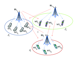
Figure 1: Interference Broadcast network.

Treating the intra-cell and inter-cell interference at each MT as noise, the maximum achievable rate of each user $i_{k}$ is

$$R_{i_{k}}(\mathbf{Q})\triangleq\log\det\left(\mathbf{I}+\mathbf{H}_{i_{k}k}\mathbf{Q}_{i_{k}}\mathbf{H}_{i_{k}k}^{H}\bar{\mathbf{R}}_{i_{k}}(\mathbf{Q}_{-i_{k}})^{-1}\right)$$ (5)

where $\mathbf{H}_{i_{k}l}\in\mathbb{C}^{M_{i_{k}}\times T_{l}}$ represents the channel matrix between BS $l$ and MT $i_{k}$; $\bar{\mathbf{R}}_{i_{k}}(\mathbf{Q}_{-i_{k}})\triangleq\sigma_{i_{k}}^{2}\mathbf{I}+\sum_{j\neq i}\mathbf{H}_{i_{k}k}\mathbf{Q}_{j_{k}}\mathbf{H}_{i_{k}k}^{H}+\sum_{l\neq k}\sum_{j=1}^{I_{l}}\mathbf{H}_{i_{k}l}\mathbf{Q}_{j_{l}}\mathbf{H}_{i_{k}l}^{H}$ is the covariance matrix of the Gaussian thermal noise (assumed to be white w.l.o.g., otherwise one can always pre-whiten the channel matrices) plus the intra-cell (second term) and inter-cell (last term) interference; and we denoted $\mathbf{Q}_{-i_{k}}\triangleq(\mathbf{Q}_{j_{l}})_{(j,l)\neq(i,k)}$ and $\mathbf{Q}\triangleq(\mathbf{Q}_{k})_{k=1}^{K}.$ Accordingly, with slight abuse of notation, we will write $\mathbf{Q}\in\mathcal{Q}$ to mean $\mathbf{Q}_{k}\in\mathcal{Q}_{k}$ for all $k\in\mathcal{K}_{\text{{BS}}}$.
Rate profile maximization. Max-min fairness has long been considered an important design criterion for wireless networks. Here we introduce the following more general rate-profile maximization: given the profile ${\boldsymbol{\alpha}}\triangleq(\alpha_{i_{k}})_{i_{k}\in\mathcal{I}}$, with each $\alpha_{i_{k}}>0$ and $\sum_{i_{k}\in\mathcal{I}}\alpha_{i_{k}}=1$, let

$$\begin{array}[]{cl}\underset{\mathbf{Q}}{\textrm{max}}&U(\mathbf{Q})\triangleq{\displaystyle\min_{i_{k}\in\mathcal{I}}}\,{\displaystyle\frac{R_{i_{k}}\left(\mathbf{Q}\right)}{\alpha_{i_{k}}}}\\ \textrm{s.t.}&\mathbf{Q}\in\mathcal{Q}.\end{array}\vspace{-.1cm} \mathcal{P}$$ ()

Special instances of this formulation have been proved to be NP-hard (see, e.g., [18]); therefore in the following our focus is on computing efficiently (d-)stationary solutions of $\mathcal{P}$.

Definition 1 (d-stationarity).

Given $\mathbf{Q}$ and $\mathbf{D}\triangleq(\mathbf{D}_{k}\mathbf{)}_{k=1}^{K}$, with $\mathbf{D}_{k}\triangleq(\mathbf{D}_{i_{k}})_{i=1}^{I_{k}}$ and $\mathbf{D}_{i_{k}}\in\mathbb{{C}}^{T_{k}\times T_{k}}$, let $U^{\prime}\!\left(\mathbf{Q};\mathbf{D}\right)$ denote the directional derivative of $U$ at $\mathbf{Q}\in\mathcal{Q}$ in the direction $\mathbf{D}$, defined as

$$U^{\prime}\!\left(\mathbf{Q};\mathbf{D}\right)\triangleq{\displaystyle\lim_{t\downarrow 0}\dfrac{{U(\mathbf{Q}+t\mathbf{D})}-U(\mathbf{Q})}{t}.}$$

A tuple $\mathbf{Q^{\star}}$ is a d-stationary solution of $\mathcal{P}$ if

$$U^{\prime}\!(\mathbf{Q}^{\star};\mathbf{Q}-\mathbf{Q}^{\star})\leq 0,\quad\forall\mathbf{Q}\in\mathcal{Q}.\vspace{-.3cm}$$ (6)

Of course, (local/global) optimal solutions of $\mathcal{P}$ satisfy (6).

Equivalent smooth reformulation: To compute d-stationary solutions of the nonconvex and nonsmooth problem $\mathcal{P}$, we preliminarily rewrite $\mathcal{P}$ in an equivalent smooth (still nonconvex) form: introducing the slack variables $R\geq 0,$ we have

$$\begin{array}[]{cl}\underset{\mathbf{Q},R\geq 0}{\textrm{max}}&R\\ \textrm{\ s.t.}&\mathbf{Q}\in\mathcal{Q}\vskip 3.0pt plus 1.0pt minus 1.0pt\\ &\hskip 1.9919ptR_{i_{k}}(\mathbf{Q})\geq\alpha_{i_{k}}R,\;\,\forall i_{k}\in\mathcal{I}.\vspace{-0.1cm}\end{array} \mathcal{P}_{s}$$ ()

We denote by $\mathcal{Z}$ the feasible set of $\mathcal{P}_{s}$. Problems $\mathcal{P}$ and $\mathcal{P}_{s}$ are equivalent in the following sense.

Proposition 2.

Given $\mathcal{P}$ and $\mathcal{P}_{s}$, the following hold:

(i)

Every feasible point of $\mathcal{P}_{s}$ is regular [i.e., it satisfies the Mangasarian-Fromovitz Constraint Qualification (MFCQ)];

(ii)

$\mathbf{Q}^{\star}$ is a d-stationary solution of $\mathcal{P}$ if and only if there exists $R^{\star}$ such that $\left(\mathbf{Q}^{\star},R^{\star}\right)$ is a stationary solution of $\mathcal{P}_{s}$.

Proof:

See supporting material. ∎

Proposition 2 opens the way to the computation of d-stationary solutions of $\mathcal{P}$ while designing algorithms for the smooth (nonconvex) formulation $\mathcal{P}_{s}$. We are not aware of any algorithm with provable convergence to d-stationary solutions of $\mathcal{P}$, as documented next.

II-B Related works

Several resource allocation problems have been studied in the literature for the vector Gaussian Interference Channel (IC), modeling multiuser interference networks. Some representative examples corresponding to different design criteria are: i) the sum-rate maximization problem [11, 12, 13, 21]; ii) the minimization of the transmit power subject to QoS constraints [7, 27]; iii) the weighted Mean-Square-Error (MSE) minimization and the min-max MSE fairness design [30, 31]; and iv) the rate profile optimization over MISO/SIMO [14, 16, 17, 32] and MIMO (single-stream) [15, 33] ICs. Since the IC is a special case of the IBC model, algorithms in [14, 15, 17] along with their convergence analysis cannot be applied to Problem $\mathcal{P}_{s}$ (and thus $\mathcal{P}$). Moreover, they are all centralized.
Related to Problem $\mathcal{P}$ is the max-min fairness formulation recently considered in [18]. There are however several differences between [18] and our approach. First, the formulation in [18] is a special case of Problem $\mathcal{P}$, corresponding to equal $\alpha_{i_{k}}$ and standard power constrains (i.e., without the additional constraints $\mathcal{W}_{k}$). Hence, the algorithm in [18] and its convergence analysis do not apply to $\mathcal{P}$. Second, even in the simplified setting considered in [18], the algorithm therein is not proved to converge to a (d-)stationary solution of the max-min fairness formulation, but to critical points of an auxiliary smooth problem that however might not be stationary for the original problem. Our algorithmic framework instead is guaranteed to converge to stationary solutions of $\mathcal{P}_{s}$ and thus, by Proposition 2, to d-stationary solutions of $\mathcal{P}$. Third, the algorithm in [18] is centralized.

The analysis of the literature shows that Problem $\mathcal{P}$ (and $\mathcal{P}_{s}$) remains unexplored in its generality. The main contribution of this section is to propose the first (distributed) algorithmic framework with provable convergence to d-stationary solutions of $\mathcal{P}$. More specifically, building on the iNner cOnVex Approximation (NOVA) framework developed in Part I [3], we propose next three alternative convexifications of the nonconvex constraints in $\mathcal{P}_{s}$, which lead to different convex subproblems [cf. (2)] and algorithms [cf. (3)]. We start in Sec. II-C with a centralized instance, while two alternative distributed implementations are derived in Sec. II-D. We remark from the outset that all the convexifications we are going to introduce satisfy Assumptions 2 and 3 (or 3 and 4) in [3], implying [together with Proposition 2(b)] convergence of the our algorithms.

II-C Centralized solution method

The nonconvexity of Problem $\mathcal{P}_{s}$ is due to the nonconvex rate constraints $R_{i_{k}}(\mathbf{Q})\geq\alpha_{i_{k}}R.$ Exploiting the concave-convex structure of the rate function

$$R_{i_{k}}(\mathbf{Q})=f_{i_{k}}^{+}(\mathbf{Q})-f_{i_{k}}^{-}(\mathbf{Q}_{-i_{k}}),\vspace{-0.1cm}$$ (7)

where $f_{i_{k}}^{+}(\mathbf{Q})=\log\det\left(\bar{\mathbf{R}}_{i_{k}}(\mathbf{Q}_{-i_{k}})+\mathbf{H}_{i_{k}k}\mathbf{Q}_{i_{k}}\mathbf{H}_{i_{k}k}^{H}\right)$ and
$f_{i_{k}}^{-}(\mathbf{Q}_{-i_{k}})=\log\det(\bar{\mathbf{R}}_{i_{k}}(\mathbf{Q}_{-i_{k}}))$ are concave functions, a tight concave lower bound of $R_{i_{k}}(\mathbf{Q})$ (satisfying Assumptions 2-4 in [3]) is naturally obtained by retaining in (7) the concave part $f_{i_{k}}^{+}$ and linearizing the convex function $-f_{i_{k}}^{-}$, which leads to the following rate approximation functions: given $\mathbf{Q}^{\nu}\triangleq(\mathbf{Q}_{i_{k}}^{\nu})_{i_{k}\in\mathcal{I}}$, with each $\mathbf{Q}_{i_{k}}^{\nu}\succeq\mathbf{0}$,

$${R}_{i_{k}}(\mathbf{Q})\geq\widetilde{R}_{i_{k}}(\mathbf{Q};\mathbf{Q}^{\nu})\triangleq{f_{i_{k}}^{+}}(\mathbf{Q})-\tilde{f}_{i_{k}}^{-}(\mathbf{Q}_{-i_{k}};\mathbf{Q}^{\nu})\vspace{-0.1cm}$$ (8)

with

$$\begin{array}[]{l}\tilde{f}_{i_{k}}^{-}(\mathbf{Q}_{-i_{k}};\mathbf{Q}^{\nu})\vskip 3.0pt plus 1.0pt minus 1.0pt\\ {\displaystyle\triangleq{f_{i_{k}}^{-}}(\mathbf{Q}_{-i_{k}}^{\nu})+\sum_{(j,l)\neq(i,k)}\!}\!\!\!\!\left<\boldsymbol{\Pi}_{i_{k}\,j_{l}}^{\,-}(\mathbf{Q}_{-i_{k}}^{\nu}),\mathbf{Q}_{j_{l}}-\mathbf{Q}_{j_{l}}^{\nu}\right>\end{array},$$ (9)

where $\left<\mathbf{A},\mathbf{B}\right>\!\triangleq\!\text{Re}\{\text{tr}(\mathbf{A}^{H}\!\mathbf{B})\}$, and we denoted by $\boldsymbol{\Pi}_{i_{k}\,j_{l}}^{\,-}(\mathbf{Q}_{-i_{k}}^{\nu})\triangleq\nabla_{\mathbf{Q}_{j_{l}}^{*}}f_{i_{k}}^{-}(\mathbf{Q}_{-i_{k}}^{\nu})=\mathbf{H}_{i_{k}l}^{H}\bar{\mathbf{R}}_{i_{k}}^{-1}(\mathbf{Q}_{-i_{k}}^{\nu})\mathbf{H}_{i_{k}l}$ the conjugate gradient of $f_{i_{k}}^{-}$ w.r.t. $\mathbf{Q}_{jl}$ [34].
Given $\mathbf{Z}^{\nu}\triangleq(\mathbf{Q}^{\nu},R^{\nu})\in\mathcal{Z}$ and $\tau_{R},\,\tau_{\mathbf{Q}}>0$, the convex approximation of problem $\mathcal{P}_{s}$ [cf. (2)] reads

$$\begin{array}[]{ccc}\hat{\mathbf{Z}}(\mathbf{Z}^{\nu})\triangleq&\!\!\underset{\mathbf{Q},\,R\geq 0}{\textrm{argmax}}&\!\!\!\!\!\left\{R-{\displaystyle{\frac{\tau_{R}}{2}}(R-R^{\nu})^{2}}-\tau_{\mathbf{Q}}\left\|\mathbf{Q}-\mathbf{Q}^{\nu}\right\|_{F}^{2}\right\}\\ &\textrm{\,\,s.t.}&\!\!\!\!\mathbf{Q}\in\mathcal{Q}\vskip 3.0pt plus 1.0pt minus 1.0pt\hfill\\ &&\!\!\!\!\widetilde{R}_{i_{k}}(\mathbf{Q};\mathbf{Q}^{\nu})\geq\alpha_{i_{k}}R,\;\forall i_{k}\in\mathcal{I},\vspace{-0.1cm}\hfill\end{array}$$ (10)

where the the quadratic terms in the objective function are added to make it strongly convex (see [3, Assumption B1]); and we denoted by $\hat{\mathbf{Z}}(\mathbf{Z}^{\nu})$ the unique solution of (10). Stationary solutions of Problem $\mathcal{P}_{s}$ can be then computed solving the sequence of convexified problems (10) via (3); the formal description of the scheme is given in Algorithm 1, whose convergence is stated in Theorem 3; the proof of the theorem follows readily from Proposition 2 and [3, Th.2].

Data: $\tau_{R},\tau_{\mathbf{Q}}>0$, $\mathbf{Z}^{0}\triangleq(\mathbf{Q}^{0},R^{0})\,\in\,\mathcal{Z}$; set $\nu=0$.

(S.1) If $\mathbf{Z}^{\nu}$ is a stationary solution of ($\mathcal{P}_{s}$): STOP.

(S.2) Compute $\hat{\mathbf{Z}}(\mathbf{Z}^{\nu})$ by (10).

(S.3) Set $\mathbf{Z}^{\nu+1}=\mathbf{Z}^{\nu}+\gamma^{\nu}(\hat{\mathbf{Z}}(\mathbf{Z}^{\nu})-\mathbf{Z}^{\nu})$ for some $\gamma^{\nu}\in(0,1]$.

(S.4) $\nu\leftarrow\nu+1$ and go to step (S.1).

Algorithm 1 : NOVA Algorithm for Problem $\mathcal{P}_{s}$ (and $\mathcal{P}$).

Theorem 3.

Let $\{\mathbf{Z}^{\nu}\triangleq(\mathbf{Q}^{\nu},R^{\nu})\}$ be the sequence generated by Algorithm 1. Choose any $\tau_{R},\tau_{\mathbf{Q}}>0$, and the step-size sequence $\{\gamma^{\nu}\}$ such that $\gamma^{\nu}\in(0,1]$, $\gamma^{\nu}\to 0,$ and $\sum_{\nu}\gamma^{\nu}=+\infty.$ Then $\{\mathbf{Z}^{\nu}\}$ is bounded and every of its limit points $\mathbf{Z}^{\infty}\triangleq(\mathbf{Q}^{\infty},R^{\infty})$ is a stationary solution of Problem $\mathcal{P}_{s}$. Therefore, $\mathbf{Q}^{\infty}$ is d-stationary for Problem $\mathcal{P}$. Furthermore, if the algorithm does not stop after a finite number of steps, none of the $\mathbf{Q}^{\infty}$ above is a local minimum of U, and thus $R^{\infty}>0$.

Theorem 3 offers some flexibility in the choice of free parameters $(\tau_{R},\tau_{Q})$ and $\{\gamma^{\nu}\}$, while guaranteeing convergence of Algorithm 1. Some effective choices for $\{\gamma^{\nu}\}$ are discussed in Part I [3]. Note also that the theorem guarantees that Algorithm 1 does not remain trapped in $R^{\infty}=0$, a “degenerate” stationary solution of $\mathcal{P}_{s}$ (the global minimizer of $\mathcal{P}_{s}$ and $\mathcal{P}$), at which some users do not receive any service.

Algorithm 1 is centralized because (10) cannot be decomposed across the base stations. This is due to the lack of separability of the rate constraints in (10): $f_{i_{k}}^{+}(\mathbf{Q})$ depends on the covariance matrices of all the users. We introduce next an alternative valid convex approximation of the nonconvex rate constraints leading to distributed schemes.

II-D Distributed implementation

A centralized implementation might not be appealing in heterogeneous multi-cell systems, where global information is not available at each BS. Distributing the computation over the cells as well as alleviating the communication overhead among the BSs is thus mandatory. This subsection addresses this issue, and it is devoted to the design of a distributed algorithm converging to d-stationary solutions of Problem $\mathcal{P}$.

By keeping the concave part $f_{i_{k}}^{+}(\mathbf{Q})$ unaltered, the approximation $\widetilde{R}_{i_{k}}$ in (8) has the desired property of preserving the structure of the original constraint function ${R}_{i_{k}}$ as much as possible. However, the structure of ${R}_{i_{k}}$ is not suited to be decomposed across the users due to the nonadditive coupling among the variables $\mathbf{Q}_{i_{k}}$ in $f_{i_{k}}^{+}(\mathbf{Q})$. To cope with this issue, the proposed idea is to introduce in $\mathcal{P}$ slack variables whose purpose is to decouple in each $f_{i_{k}}^{+}$ the covariance matrix $\mathbf{Q}_{i_{k}}$ of user $i_{k}$ from those of the other users$-$the interference term $\bar{\mathbf{R}}_{i_{k}}(\mathbf{Q}_{-i_{k}})$. More specifically, introducing the slack variables $\mathbf{Y}\triangleq(\mathbf{Y}_{k})_{k\in\mathcal{K}_{\mathtt{BS}}}$, with $\mathbf{Y}_{k}=(\mathbf{Y}_{i_{k}})_{i_{k}\in\mathcal{I}_{k}}$, and setting $\mathbf{I}_{i_{k}}(\mathbf{Q})\triangleq\sum_{l=1}^{K}\sum_{j=1}^{I_{l}}\mathbf{H}_{i_{k}l}\mathbf{Q}_{j_{l}}\mathbf{H}_{i_{k}l}^{H},$ we can write $f_{i_{k}}^{+}(\mathbf{Q})=\overline{f}_{i_{k}}^{\,+}(\mathbf{Y}_{i_{k}}),$ with $\overline{f}_{i_{k}}^{\,+}(\mathbf{Y}_{i_{k}})\triangleq\log\det(\sigma_{i_{k}}^{2}\mathbf{I}+\mathbf{Y}_{i_{k}})$ and $\mathbf{Y}_{i_{k}}=\mathbf{I}_{i_{k}}(\mathbf{Q})$. Then, in view of (7), Problem $\mathcal{P}_{s}$ can be rewritten in the following equivalent form:

$$\begin{array}[]{cl}\underset{\mathbf{Q},R\geq 0,\mathbf{Y}}{\textrm{max}}&R\\ \textrm{\vspace{-1.5cm} s.t.}&\mathbf{Q}\in\mathcal{Q},\vskip 3.0pt plus 1.0pt minus 1.0pt\\ &\overline{f}_{i_{k}}^{\,+}(\mathbf{Y}_{i_{k}})-\!f_{i_{k}}^{-}(\mathbf{Q}_{-i_{k}})\!\geq\!\alpha_{i_{k}}R,\ \forall i_{k}\in\mathcal{I},\vskip 3.0pt plus 1.0pt minus 1.0pt\\ &\mathbf{0}\preceq\mathbf{Y}_{i_{k}}\preceq\mathbf{I}_{i_{k}}(\mathbf{Q}),\ \forall i_{k}\in\mathcal{I}.\vspace{-0.1cm}\end{array} \mathcal{P}_{s}^{{}^{\prime}}$$ ()

The next proposition states the formal connection between $\mathcal{P}_{s}^{{}^{\prime}}$ and $\mathcal{P}_{s}$, whose proof is omitted because of space limitations.

Proposition 4.

Given $\mathcal{P}_{s}$ and $\mathcal{P}_{s}^{{}^{\prime}}$, the following hold:

(i)

Every feasible point $\left(\mathbf{Q},R,\mathbf{Y}\right)$ of $\mathcal{P}_{s}^{{}^{\prime}}$ satisfies the MFCQ;

(ii)

$\left(\mathbf{Q}^{\star},R^{\star}\right)$ is a stationary solution of $\mathcal{P}_{s}$ if and only if there exists $\mathbf{Y}^{\star}$ such that $\left(\mathbf{Q}^{\star},R^{\star},\mathbf{Y}^{\star}\right)$ is a stationary solution of $\mathcal{P}_{s}^{{}^{\prime}}$.

It follows from Propositions 2 and 4 that, to compute d-stationary solutions of $\mathcal{P}$, we can focus w.l.o.g on $\mathcal{P}_{s}^{{}^{\prime}}$. Using (9), we can minorize the left-hand side of the rate constraints in $\mathcal{P}_{s}^{{}^{\prime}}$ as

$$\begin{array}[]{cc}\overline{f}_{i_{k}}^{\,+}(\mathbf{Y}_{i_{k}})-\!f_{i_{k}}^{-}(\mathbf{Q}_{-i_{k}})\geq&\widehat{R}_{i_{k}}\left(\mathbf{Q}_{-i_{k}},\mathbf{Y}_{i_{k}};\mathbf{Q}^{\nu}\right)\hfill\\ \hfill\triangleq&\overline{f}_{i_{k}}^{\,+}(\mathbf{Y}_{i_{k}})-\widetilde{f}_{i_{k}}^{-}\left(\mathbf{Q}_{-i_{k}};\mathbf{Q}^{\nu}\right).\end{array}$$

The approximation of Problem $\mathcal{P}_{s}^{{}^{\prime}}$ becomes [cf. (2)]: given a feasible $\mathbf{W}^{\nu}\triangleq\left(\mathbf{Q}^{\nu},R^{\nu},\mathbf{Y}^{\nu}\right)$, and any $\tau_{\mathbf{Q}},\tau_{R},\tau_{\mathbf{Y}}>0$,

$$\!\!\!\!\!\!\begin{array}[]{ccl}\begin{array}[]{c}\hat{\mathbf{W}}(\mathbf{W}^{\nu})\triangleq\\ \\ \end{array}\!\!\!\!\!\!\!&\!\!\!\begin{array}[]{c}\underset{\mathbf{Q},\,R\geq 0,\,\mathbf{Y}}{\textrm{argmax}}\\ \\ \end{array}\!\!\!\!\!\!\!&\!\!\!\begin{array}[]{c}\left\{R-{\displaystyle\frac{\tau_{R}}{2}}\left(R-R^{\nu}\right)^{2}\right.\hfill\\ \left.-\tau_{\mathbf{Q}}\left\|\mathbf{Q}-\mathbf{Q}^{\nu}\right\|_{F}^{2}-\tau_{\mathbf{Y}}\left\|\mathbf{Y}-\mathbf{Y}^{\nu}\right\|_{F}^{2}\right\}\end{array}\\ \!\!\!\!\!\!\!&\!\textrm{ \vspace{-1.6cm} s.t.}\!\!\!\!\!\!\!&\mathbf{Q}\in\mathcal{Q},\vskip 3.0pt plus 1.0pt minus 1.0pt\\ \!\!\!\!\!\!\!&\!\!\!\!\!\!\!\!&\widehat{R}_{i_{k}}\left(\mathbf{Q}_{-i_{k}},\,\mathbf{Y}_{i_{k}};\mathbf{Q}^{\nu}\right)\geq\alpha_{i_{k}}R,\ \forall i_{k}\in\mathcal{I},\vskip 3.0pt plus 1.0pt minus 1.0pt\\ \!\!\!\!\!\!\!&\!\!\!\!\!\!\!\!&\mathbf{0}\preceq\mathbf{Y}_{i_{k}}\preceq\mathbf{I}_{i_{k}}(\mathbf{Q}),\ \forall i_{k}\in\mathcal{I}.\end{array}$$ (11)

To compute d-stationary solutions of Problem $\mathcal{P}$ via (11), we can invoke Algorithm 1 wherein the $\mathbf{Z}$ variables [resp. $\hat{\mathbf{Z}}(\mathbf{Z}^{\nu})$ in Step 2] are replaced by the $\mathbf{W}$ ones [resp. $\hat{\mathbf{W}}(\mathbf{W}^{\nu})$, defined in (11)]. Convergence of this new algorithm is still given by Theorem 3. The difference with the centralized approach in Sec. II-C is that now, thanks to the additively separable structure of the objective and constraint functions in (11), one can compute $\hat{\mathbf{W}}$ in a distributed way, by leveraging standard dual decomposition techniques; which is shown next.

With $\mathbf{W}\triangleq\left(\mathbf{Q},R,\mathbf{Y}\right)$, denoting $\boldsymbol{\lambda}\triangleq\left(\lambda_{i_{k}}\right)_{i_{k}\in\mathcal{I}}$ and $\boldsymbol{\Omega}\triangleq(\boldsymbol{\Omega}_{i_{k}})_{i_{k}\in\mathcal{I}}$ the multipliers associated to the rate constraints $\widehat{R}_{i_{k}}(\mathbf{Q}_{-i_{k}},\,\mathbf{Y}_{i_{k}};\mathbf{Q}^{\nu})\geq\alpha_{i_{k}}R$ and slack variable constraints $\mathbf{Y}_{i_{k}}\preceq\mathbf{I}_{i_{k}}(\mathbf{Q})$ respectively, let us define the (partial) Lagrangian of (11) as

$$\!\!\!\!\!\!\!\!\begin{array}[]{l}\mathcal{L}(\mathbf{W},\boldsymbol{\lambda},\boldsymbol{\Omega};\mathbf{W}^{\nu})\triangleq\mathcal{L}_{R}(R,\boldsymbol{\lambda};R^{\nu})+\sum_{k=1}^{K}\mathcal{L}_{\mathbf{Q}_{k}}(\mathbf{Q}_{k},\boldsymbol{\lambda},\boldsymbol{\Omega};\mathbf{Q}^{\nu})\\ \hskip 85.35826pt+\sum_{k=1}^{K}\mathcal{L}_{\mathbf{Y}_{k}}(\mathbf{Y}_{k},\boldsymbol{\lambda},\boldsymbol{\Omega};\mathbf{Y}^{\nu})\end{array}\vskip 3.0pt plus 1.0pt minus 1.0pt$$

where

$$\!\!\!\!\!\!\!\!\mathcal{L}_{R}(R,\boldsymbol{\lambda};R^{\nu})\triangleq-R+{\displaystyle\frac{\tau_{R}}{2}}(R-R^{\nu})^{2}+\boldsymbol{\boldsymbol{\lambda}}^{T}\boldsymbol{\alpha}R;$$

$$\begin{array}[]{l}\!\!\!\!\!\!\mathcal{L}_{\mathbf{Q}_{k}}(\mathbf{Q}_{k},\boldsymbol{\boldsymbol{\lambda}},\boldsymbol{\Omega};\mathbf{Q}^{\nu})\triangleq\tau_{\mathbf{Q}}\left\|\mathbf{Q}_{k}-\mathbf{Q}_{k}^{\nu}\right\|_{F}^{2}+\sum_{i_{k}\in\mathcal{I}_{k}}\lambda_{i_{k}}f_{i_{k}}^{-}(\mathbf{Q}_{-i_{k}}^{\nu})\vskip 6.0pt plus 2.0pt minus 2.0pt\\ \qquad\qquad+\sum_{i_{k}\in\mathcal{I}_{k}}\sum_{(j,l)\neq(i,k)}\!\left\langle\lambda_{j_{l}}\boldsymbol{\Pi}_{j_{l}\,i_{k}}^{-}(\mathbf{Q}_{-j_{l}}^{\nu}),\mathbf{Q}_{i_{k}}-\mathbf{Q}_{i_{k}}^{\nu}\right\rangle\vskip 3.0pt plus 1.0pt minus 1.0pt\\ \qquad\qquad-\sum_{i_{k}\in\mathcal{I}_{k}}\left\langle\sum_{j_{l}\in\mathcal{I}}\mathbf{H}_{j_{l}k}^{H}\boldsymbol{\Omega}_{j_{l}}\mathbf{H}_{j_{l}k},\mathbf{Q}_{i_{k}}\right\rangle;\end{array}$$

$$\!\!\!\!\!\begin{array}[]{l}\mathcal{L}_{\mathbf{Y}_{k}}(\mathbf{Y}_{k},\boldsymbol{\lambda},\boldsymbol{\Omega};\mathbf{Y}^{\nu})\triangleq\tau_{\mathbf{Y}}\left\|\mathbf{Y}_{k}-\mathbf{Y}_{k}^{\nu}\right\|_{F}^{2}+\sum_{i_{k}\in\mathcal{I}_{k}}\left\langle\boldsymbol{\Omega}_{i_{k}},\mathbf{Y}_{i_{k}}\right\rangle\vskip 6.0pt plus 2.0pt minus 2.0pt\\ \qquad\qquad\qquad-\sum_{i_{k}\in\mathcal{I}_{k}}\lambda_{i_{k}}\log\det(\sigma_{i_{k}}^{2}\mathbf{I}+\mathbf{Y}_{i_{k}}),\end{array}$$

with $\boldsymbol{\alpha}\triangleq(\alpha_{i_{k}})_{i_{k}\in\mathcal{I}}$. The additively separable structure of $\mathcal{L}(\mathbf{W},\boldsymbol{\lambda},\boldsymbol{\Omega};\mathbf{W}^{\nu})$ leads to the following decomposition of the dual function:

$$\begin{array}[]{lll}D(\boldsymbol{\lambda},\boldsymbol{\Omega};\mathbf{W}^{\nu})\triangleq&{\displaystyle\min_{R\geq 0}}\;\mathcal{L}_{R}(R,\boldsymbol{\lambda};R^{\nu})\\ &+\sum_{k=1}^{K}{\displaystyle\min_{\mathbf{Q}_{k}\in\mathcal{Q}_{k}}}\mathcal{L}_{\mathbf{Q}_{k}}(\mathbf{Q}_{k},\boldsymbol{\lambda},\boldsymbol{\Omega};\mathbf{Q}^{\nu})\\ &+\sum_{k=1}^{K}{\displaystyle\min_{(\mathbf{Y}_{i_{k}}\succeq\mathbf{0})_{i_{k}\in\mathcal{I}_{k}}}}\mathcal{L}_{\mathbf{Y}_{k}}(\mathbf{Y}_{k},\boldsymbol{\lambda},\boldsymbol{\Omega};\mathbf{Y}^{\nu}).\hfill\end{array}$$ (12)

The unique solutions of the above optimization problems are denoted by $R^{\star}(\boldsymbol{\lambda};R^{\nu})={\displaystyle\text{{argmin}}_{R\geq 0}}\mathcal{L}_{R}(R,\boldsymbol{\lambda};R^{\nu})$, $\mathbf{Q}_{k}^{\star}(\boldsymbol{\lambda},\boldsymbol{\Omega};\mathbf{Q}^{\nu})={\displaystyle\text{{argmin}}_{\mathbf{Q}_{k}\in\mathcal{Q}_{k}}}$$\mathcal{L}_{\mathbf{Q}_{k}}(\mathbf{Q}_{k},\boldsymbol{\lambda},\boldsymbol{\Omega};\mathbf{Q}^{\nu})$, and $\mathbf{Y}_{k}^{\star}(\boldsymbol{\lambda},\boldsymbol{\Omega};\mathbf{Y}^{\nu})={\displaystyle\text{{argmin}}_{(\mathbf{Y}_{i_{k}}\succeq\mathbf{0})_{i_{k}\in\mathcal{I}_{k}}}}$$\mathcal{L}_{\mathbf{Y}_{k}}(\mathbf{Y}_{k},\boldsymbol{\lambda},\boldsymbol{\Omega};\mathbf{Y}^{\nu})$. We show next that $R^{\star}$ and $\mathbf{Y}_{k}^{\star}$ have a closed form expression, and so does $\mathbf{Q}_{k}^{\star}$, when the feasible sets $\mathcal{Q}_{k}$ contain only power budget constraints [i.e., there is no set $\mathcal{W}_{k}$ in (4)], a fact that will be tacitly assumed hereafter (the quite standard proof of Lemma 5 is omitted because of space limitations).

Lemma 5 (Closed form of $R^{\star}(\boldsymbol{\lambda};R^{\nu})$).

The optimal solution $R^{\star}(\boldsymbol{\lambda};R^{\nu})$ has the following expression

$$R^{\star}(\boldsymbol{\lambda};R^{\nu})=\left[R^{\nu}-\frac{\boldsymbol{\lambda}^{T}\boldsymbol{\alpha}-1}{\tau_{R}}\right]_{+},\vspace{-0.1cm}$$ (13)

where $[\mathbf{x}]_{+}\triangleq\max(\mathbf{0},\mathbf{x})$ (applied component-wise).

Lemma 6 (Closed form of $\mathbf{Q}_{k}^{\star}(\boldsymbol{\lambda},\boldsymbol{\Omega};\mathbf{Q}^{\nu})$).

Let $\mathbf{U}_{i_{k}}^{\nu}\mathbf{D}_{i_{k}}^{\nu}\mathbf{U}_{i_{k}}^{{}^{\nu}\,H}$ be the eigenvalue/eigenvector decomposition of $2\tau_{\mathbf{Q}}\mathbf{Q}_{i_{k}}^{\nu}-\sum_{(j,l)\neq(i,k)}\lambda_{j_{l}}\boldsymbol{\Pi}_{j_{l}\,i_{k}}^{-}\left(\mathbf{Q}_{-j_{l}}^{\nu}\right)+\sum_{j_{l}\in\mathcal{I}}\mathbf{H}_{j_{l}k}^{H}\boldsymbol{\Omega}_{j_{l}}\mathbf{H}_{j_{l}k}$ with $\mathbf{D}_{i_{k}}^{\nu}\triangleq\textrm{\emph{\text{{Diag}}}}(\mathbf{d}_{i_{k}}^{\nu})$. Let us partition the optimal solution $\mathbf{Q}_{k}^{\star}(\boldsymbol{\lambda},\boldsymbol{\Omega};\mathbf{Q}^{\nu})\triangleq(\mathbf{Q}_{i_{k}}^{\star}(\boldsymbol{\lambda},\boldsymbol{\Omega};\mathbf{Q}^{\nu}))_{i_{k}\in\mathcal{I}_{k}}$. Then each $\mathbf{Q}_{i_{k}}^{\star}(\boldsymbol{\lambda},\boldsymbol{\Omega};\mathbf{Q}^{\nu})$ has the following waterfilling-like expression [we omit the dependence on $(\boldsymbol{\lambda},\boldsymbol{\Omega};\mathbf{Q}^{\nu})$]

$$\mathbf{Q}_{i_{k}}^{\star}=\mathbf{U}_{{i_{k}}}^{\nu}\textrm{\emph{\text{{Diag}}}}\!\left(\left[\frac{\mathbf{d}_{i_{k}}^{\nu}-\xi_{k}^{\star}}{2\tau_{\mathbf{Q}}}\right]_{+}\right)\mathbf{U}_{{i_{k}}}^{\nu\,H},\ \forall i_{k}\in\mathcal{I}_{k},$$ (14)

where $\xi_{k}^{\star}\geq 0$ is the water-level chosen to satisfy the power constraint $\sum_{i_{k}\in\mathcal{I}_{k}}^{I_{k}}\text{tr}(\mathbf{Q}_{i_{k}}^{\star})\leq P_{k}$, which can be found either exactly by the finite-step hypothesis method (see Algorithm 4, Appendix -A) or approximately via bisection on the interval $\left[0,\sum_{i_{k}\in\mathcal{I}_{k}}\textrm{tr}\left(\textrm{\emph{\text{{Diag}}}}(\mathbf{d}_{i_{k}}^{\nu})\right)/(T_{k}\,I_{k})\right]$.

Proof:

See Appendix -A.∎

Lemma 7 (Closed form of $\mathbf{Y}_{k}^{\star}(\boldsymbol{\lambda},\boldsymbol{\Omega};\mathbf{Y}^{\nu})$).

Let $\mathbf{V}_{i_{k}}^{\nu}\mathbf{D}_{i_{k}}^{\nu}\mathbf{V}_{i_{k}}^{\nu H}$ be the eigenvalue/eigenvector decomposition of $2\tau_{\mathbf{Y}}\mathbf{Y}_{i_{k}}^{\nu}-\boldsymbol{\Omega}_{i_{k}}^{\nu}$, with $\mathbf{D}_{i_{k}}^{\nu}=\textrm{{\emph{\text{{Diag}}}}}(\mathbf{d}_{i_{k}}^{\nu})$. Let us partition the optimal solution $\mathbf{Y}_{k}^{\star}(\boldsymbol{\lambda},\boldsymbol{\Omega};\mathbf{Y}^{\nu})\triangleq(\mathbf{Y}_{i_{k}}^{\star}(\boldsymbol{{\lambda}}_{i_{k}},\boldsymbol{\Omega}_{i_{k}};\mathbf{Y}^{\nu}))_{i_{k}\in\mathcal{I}_{k}}$. Then, each $\mathbf{Y}_{i_{k}}^{\star}(\boldsymbol{{\lambda}}_{i_{k}},\boldsymbol{\Omega}_{i_{k}};\mathbf{Y}^{\nu})$ has the following expression [we omit the dependence on $(\boldsymbol{\lambda}_{i_{k}},\boldsymbol{\Omega}_{i_{k}};\mathbf{Y}^{\nu})$]

$$\mathbf{Y}_{i_{k}}^{\star}=\mathbf{V}_{i_{k}}^{\nu}\textrm{\emph{\text{{Diag}}}}\left(\mathbf{y}_{i_{k}}^{\nu}\right)\mathbf{V}_{i_{k}}^{\nu H},\ \forall i_{k}\in\mathcal{I}_{k},$$ (15)

with

$$\begin{array}[]{cc}\mathbf{y}_{i_{k}}^{\nu}\triangleq&\left[-{\displaystyle\frac{1}{2}\left(\mathbf{\sigma}_{i_{k}}^{2}-\frac{1}{2\tau_{\mathbf{Y}}}\mathbf{d}_{i_{k}}^{\nu}\right)}\right.\hfill\vskip 3.0pt plus 1.0pt minus 1.0pt\\ &\left.+{\displaystyle\frac{1}{2}\sqrt{\left(\mathbf{\sigma}_{i_{k}}^{2}+\frac{1}{2\tau_{\mathbf{Y}}}\mathbf{d}_{i_{k}}^{\nu}\right)^{2}+\frac{2\lambda_{i_{k}}}{\tau_{\mathbf{Y}}}\,\mathbf{1}}}\,\right]_{+},\vspace{-0.1cm}\end{array}$$ (16)

where $\mathbf{1}$ denotes the vector of all ones.

Proof:

See Appendix -B. ∎

Finally, note that, since $\mathcal{L}\left(\mathbf{W},\boldsymbol{\lambda},\boldsymbol{\Omega};\mathbf{W}^{\nu}\right)$ is strongly convex for any given $\boldsymbol{\lambda}\geq\mathbf{0}$ and $\boldsymbol{\Omega}\triangleq\left(\boldsymbol{\Omega}_{i_{k}}\succeq\mathbf{0}\right)_{i_{k}\in\mathcal{I}}$, the dual function $D(\boldsymbol{\lambda},\boldsymbol{\Omega};\mathbf{W}^{\nu})$ in (12) is ($\mathbb{{R}}$-)differentiable on $\mathbb{{R}}_{+}^{I}\times\prod_{i_{k}\in\mathcal{I}}\mathbb{C}^{M_{i_{k}}\times M_{i_{k}}}$, with (conjugate) gradient given by

$$\begin{array}[]{c}\begin{array}[]{cc}\nabla_{\boldsymbol{\lambda}_{i_{k}}}D(\boldsymbol{\lambda},\boldsymbol{\Omega};\mathbf{W}^{\nu})=&\alpha_{i_{k}}R^{\star}-\widehat{R}_{i_{k}}\left(\mathbf{Q}_{-i_{k}}^{\star},\,\mathbf{Y}_{i_{k}}^{\star};\mathbf{Q}^{\nu}\right)\end{array}\\ \nabla_{\boldsymbol{\Omega}_{i_{k}}^{*}}D(\boldsymbol{\lambda},\boldsymbol{\Omega};\mathbf{W}^{\nu})=\mathbf{Y}_{i_{k}}^{\star}-\sum_{j_{l}\in\mathcal{I}}\mathbf{H}_{i_{k}l}\mathbf{Q}_{j_{l}}^{\star}\mathbf{H}_{i_{k}l}^{H},\end{array}$$ (17)

where $R^{\star}$, $\mathbf{Q}_{i_{k}}^{\star}$, and $\mathbf{Y}_{i_{k}}^{\star}$ are given by (13), (14), and (15), respectively. Also, it can be shown that the dual function is $\mathcal{C}^{2}$, with Lipschitz continuous (augmented) Hessian with respect to $\mathbf{W}^{\nu}$. Then, the dual problem

$$\max_{\underset{\boldsymbol{\Omega}=(\boldsymbol{\Omega}_{i_{k}}\succeq\mathbf{0})_{i_{k}\in\mathcal{I}}}{\boldsymbol{\lambda}\geq\mathbf{0}\vskip 3.0pt plus 1.0pt minus 1.0pt}}D(\boldsymbol{\lambda},\boldsymbol{\Omega};\mathbf{W}^{\nu})\vspace{-0.1cm}$$ (18)

can be solved using either first or second order methods. A gradient-based scheme with diminishing step-size is given in Algorithm 2, whose convergence is stated in Theorem 8 (the proof of the theorem follows from classical arguments and thus is omitted). In Algorithm 2, $P_{\mathbb{{H}}_{+}}(\mathbf{\bullet})$ denotes the orthogonal projection onto the set of complex positive semidefinite (and thus Hermitian) matrices.

Algorithm 2 Distributed dual algorithm solving (18)

Data: $\mathbf{\boldsymbol{\lambda}}^{0}\triangleq(\lambda_{i_{k}}^{0})_{i_{k}\in\mathcal{I}}\geq\mathbf{0}$, $\boldsymbol{\Omega}^{0}\triangleq(\boldsymbol{\Omega}_{i_{k}}^{0}\succeq\mathbf{0})_{i_{k}\in\mathcal{I}}$, $\mathbf{W}^{\nu}=(\mathbf{Q}^{\nu},R^{\nu},\mathbf{Y}^{\nu})$. Set $n=0$.

(S.1) If $\mathbf{\boldsymbol{{\lambda}}}^{n}$ and $\boldsymbol{\Omega}^{n}$ satisfy a suitable termination criterion: STOP.

(S.2) Compute each $R^{\star}(\boldsymbol{\lambda}^{n};R^{\nu})$, $\mathbf{Q}_{i_{k}}^{\star}(\boldsymbol{\lambda}^{n},\boldsymbol{\Omega}^{n};\mathbf{Q}^{\nu})$, and $\mathbf{Y}_{i_{k}}^{\star}(\boldsymbol{\lambda}^{n},\boldsymbol{\Omega}^{n};\mathbf{Y}^{\nu})$ [cf. (13)-(15)].

(S.3) Update $\boldsymbol{\lambda}$ and $\boldsymbol{\Omega}$ according to

$$\begin{array}[]{c}\lambda_{i_{k}}^{n+1}=\left[\lambda_{i_{k}}^{n}+\beta^{n}\nabla_{\lambda_{i_{k}}}D(\boldsymbol{\lambda},\boldsymbol{\Omega};\mathbf{W}^{\nu})\right]_{+}\\ \boldsymbol{\Omega}_{i_{k}}^{n+1}=P_{\mathbb{{H}}_{+}}\left(\boldsymbol{\Omega}_{i_{k}}^{n}+\beta^{n}\nabla_{\boldsymbol{\Omega}_{i_{k}}^{*}}D(\boldsymbol{\lambda},\boldsymbol{\Omega};\mathbf{W}^{\nu})\right)\end{array},\ \forall i_{k}\in\mathcal{I}$$

for some $\beta^{n}>0$.

(S.4) $n\leftarrow n+1$, go back to (S.1).

Theorem 8.

Let $\left\{\left(\boldsymbol{\lambda}^{n},\boldsymbol{\Omega}^{n}\right)\right\}$ be the sequence generated by Algorithm 2. Choose the step-size sequence $\left\{\beta^{n}\right\}$ such that $\beta^{n}>0$, $\beta^{n}\rightarrow 0$, $\sum_{n}\beta^{n}=+\infty$, and $\sum_{n}\left(\beta^{n}\right)^{2}<\infty$. Then, $\left\{\left(\boldsymbol{\lambda}^{n},\boldsymbol{\Omega}^{n}\right)\right\}$ converges to a solution of (18). Therefore, the sequence $\left\{\left(R^{\star}(\boldsymbol{\lambda}^{n};R^{\nu}),\,\mathbf{Q}^{\star}\left(\boldsymbol{{\lambda}}^{n},\boldsymbol{\Omega}^{n};\mathbf{Q}^{\nu}\right),\mathbf{Y}^{\star}\left(\boldsymbol{{\lambda}}^{n},\boldsymbol{\Omega}^{n};\mathbf{Y}^{\nu}\right)\right)\right\}$ converges to the unique solution of (11).

Algorithm 2 can be implemented in a fairly distributed way across the BSs, with limited communication overhead. More specifically, given the current value of $(\boldsymbol{\lambda},\boldsymbol{\Omega})$, each BS $k$ updates individually the covariance matrices $\mathbf{Q}_{k}=(\mathbf{Q}_{i_{k}})_{i_{k}\in\mathcal{I}_{k}}$ of the users in the cell $k$ as well as the slack variables $\mathbf{Y}_{k}=(\mathbf{Y}_{i_{k}})_{i_{k}\in\mathcal{I}_{k}}$, by computing the closed form solutions $\mathbf{Q}_{i_{k}}^{\star}(\boldsymbol{\lambda}^{n},\boldsymbol{\Omega}^{n};\mathbf{Q}^{\nu})$ [cf. (14)] and $\mathbf{Y}_{i_{k}}^{\star}(\boldsymbol{\lambda}^{n},\boldsymbol{\Omega}^{n};\mathbf{Y}^{\nu})$ [cf. (15)]. The update of the $R$-variable [using $R^{\star}(\boldsymbol{\lambda};R^{\nu})$] and the multipliers $(\boldsymbol{\lambda},\boldsymbol{\Omega})$ require some coordination among the BSs: it can be either carried out by a BS header or locally by all the BSs if a consensus-like scheme is employed in order to obtain locally the information required to compute $R^{\star}(\boldsymbol{\lambda};R^{\nu})$ and the gradients in (17).

The dual problem (18) can be also solved using a second order-based scheme, which is expected in practice to be faster than a gradient-based one. It is sufficient to replace Step 3 of Algorithm 2 with the following updating rules for the multipliers:

$$\begin{split}&\boldsymbol{\lambda}^{n+1}=\boldsymbol{\boldsymbol{\lambda}}^{n}+s^{n}\left([\hat{\boldsymbol{\lambda}}^{n+1}]_{+}-\boldsymbol{\boldsymbol{\lambda}}^{n}\right),\\ &\boldsymbol{\Omega}^{n+1}=\boldsymbol{\Omega}^{n}+s^{n}\left(P_{\mathbb{{H}}_{+}}(\hat{\boldsymbol{\Omega}}^{n+1})-\boldsymbol{\Omega}^{n}\right),\end{split}$$ (19)

where $\hat{\boldsymbol{\lambda}}^{n+1}$ and $\hat{\boldsymbol{\Omega}}^{n+1}$ can be computed by $\hat{\boldsymbol{\Lambda}}^{n+1}\triangleq[\hat{\boldsymbol{\boldsymbol{\lambda}}}^{n+1},\text{vec}\!(\hat{{\boldsymbol{\Omega}}}^{n+1})^{T}]^{T}$, with $\text{vec}\!(\hat{{\boldsymbol{\Omega}}})\triangleq(\text{vec}\!(\hat{{\boldsymbol{\Omega}}})_{i_{k}})_{i_{k}\in\mathcal{I}}$, which is updated according to

$$\begin{split}\hat{\boldsymbol{\Lambda}}^{n+1}\triangleq\hat{\boldsymbol{\Lambda}}^{n}+&(\nabla_{\boldsymbol{\boldsymbol{\lambda}},\text{vec}(\boldsymbol{\Omega}^{*})}^{2}D(\boldsymbol{\boldsymbol{\lambda}}^{n},\boldsymbol{\Omega}^{n};\mathbf{W}^{\nu}))^{-1}\\ &\cdot\nabla_{\boldsymbol{\boldsymbol{\lambda}},\text{vec}(\boldsymbol{\Omega}^{*})}D(\boldsymbol{\boldsymbol{\lambda}}^{n},\boldsymbol{\Omega}^{n};\mathbf{W}^{\nu}).\end{split}$$ (20)

In Appendix -C we provide the explicit expression of the (augmented) Hessian matrices and gradients in (20).

II-E Numerical results

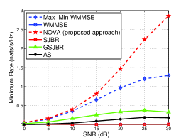
Figure 2: Minimum rate vs. SNR: The proposed algorithm reaches better solutions than the state of the art.

In this section we present some experiments assessing the effectiveness of the proposed formulation and algorithms.

Example $\#\,1:\,$Centralized algorithm. We start comparing Algorithm 1 with three other approaches presented in the literature for the resource allocation over IBCs, namely: 1) the Max-Min WMMSE [18], which aims at maximizing the minimum rate of the system (a special case of $\mathcal{P}_{s}$); 2) the WMMSE algorithm [35] and the partial linearization-based algorithm (termed SJBR) [13], which consider the maximization of the system sum-rate; and 3) the partial linearization-based algorithm [13], applied to maximize the geometric mean of the rates (the proportional fairness utility function), termed GSJBR. As benchmark, we also report the results achieved using the standard nonlinear programming solver in Matlab, specifically the active-set algorithm in ’fmincon’ (among the other options in fmincon, the active-set algorithm was the one that showed better performance); we refer to it as “AS” algorithm. To allow the comparison, we consider a special case of $\mathcal{P}_{s}$ as in [18]. We simulated a $K=4$ cell IBC with $\mathcal{I}_{k}=3$ randomly placed active MTs per cell; the BSs and MTs are equipped with 4 antennas. Channels are Rayleigh fading, whose path-loss are generated using the 3GPP(TR 36.814) methodology. We assume white zero-mean Gaussian noise at each receiver, with variance $\sigma^{2}$, and same power budget $P$ for all the BSs; the signal to noise ratio is then $\textrm{SNR}=P/\sigma^{2}$. Algorithm 1 is simulated using $\tau_{R}=1$e$-7$ and the step-size rule $\gamma^{\nu}=\gamma^{\nu-1}(1-10^{-3}\gamma^{\nu-1})$, with $\gamma^{0}=1$. The same step-size rule is used for SJBR and GSJBR. The same random feasible initialization is used for all the algorithms. All algorithms are terminated when the absolute value of the difference between two consecutive values of the objective function becomes smaller than $1e-3$. In Fig. 2 we plot the minimum rate versus SNR achieved by the aforementioned algorithms. All results are averaged over 300 independent channel/topology realizations. The figures show that our algorithm yields substantially more fair rate allocations (larger minimum rates) than all the others. As expected, we observed that SJBR and WMMSE achieve higher sum-rates (not reported in the figure) while sacrificing the fairness: SJBR and WMMSE can shut off some users (the associated minimum rate is zero). More specifically, for $\text{SNR}\sim 15$dB (resp. $\text{SNR}\sim 30$dB) we observed the following average losses on the sum-rate w.r.t. SJBR (and WMMSE): $\sim$ ​$70\%$ (resp. $\sim$ ​$45\%$) for our algorithm and Max-Min WMMSE; $\sim$ ​$50\%$ (resp. $\sim$ ​$60\%$) for GSJBR; and $\sim$ ​$80\%$ (resp. $\sim$ ​$80\%$) for AS. Between Algorithm 1 and the Max-Min WMMSE [18], the former provides better solutions, both in terms of minimum rate (cf. Fig. 2) and sum-rate (not reported). This might be due to the fact that the Max-Min WMMSE converges to stationary solutions of an auxiliary nonconvex problem (obtained lifting $\mathcal{P}_{s}$) that are not proved to be stationary also for the original formulation $\mathcal{P}$; our algorithm instead converges to d-stationary solutions of $\mathcal{P}$.

Example $\#$ 2: Distributed algorithms. We test now the distributed algorithms in Sec. II-D and compare them with the centralized implementation. Specifically, we simulate i) Algorithm 1 based on the solution $\hat{{\mathbf{W}}}(\mathbf{W}^{\nu})$ (termed Centralized algorithm); ii) the same algorithm as in i) but with $\hat{{\mathbf{W}}}(\mathbf{W}^{\nu})$ computed in a distributed way using Algorithm 2 (termed Distributed, first-order); and iii) the same algorithm as in i) but with $\hat{{\mathbf{W}}}(\mathbf{W}^{\nu})$ computed solving the dual problem (18) using a second-order method (termed Distributed, second-order). The simulated scenario as well as the tuning of the algorithms is as in Example$\,\#1$. In Algorithm 2, the step-size sequence $\{\beta^{n}\}$ has been chosen as $\beta^{n}=\beta^{n-1}(1-0.8\cdot\beta^{n-1})$; also the starting point $(\lambda^{0},\boldsymbol{{\Omega}}^{0})$ is set equal to the optimal solution $(\lambda^{\star},\boldsymbol{{\Omega}}^{\star})$ of the previous round. Fig. 3 shows the normalized rate evolution achieved by the aforementioned algorithms versus the iteration index $n$. For the distributed algorithms, the number of iterations counts both the inner and outer iterations. Note that all the algorithms converge to the same stationary point of Problem $\mathcal{P}$, and they are quite fast. As expected, exploiting second order information accelerates the practical convergence but at the cost of extra signaling among the BSs.

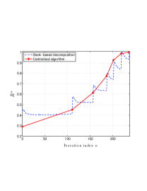
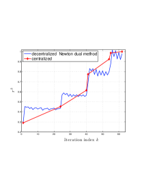
Figure 3: Minimum rate vs. iterations. Left plot: Centralized algorithm vs. Distributed, first order; Right plot: Centralized algorithm vs. Distributed, second order.

III Multigroup Multicast Beamforming

III-A System model

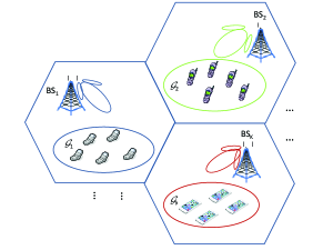
Figure 4: Multicell multi-group multicast network.

We study the general Max-Min Fair (MMF) beamforming problem for multi-group multicasting [22], where different groups of subscribers request different data streams from the transmitter; see Fig. 4.
We assume that there are $K$ BSs (one per cell), each of them equipped with $N_{t}$ transmit antennas and a total of $I$ active users, which have a single receive antenna; let $\mathcal{I}\triangleq\{1,\ldots,I\}$. For notational simplicity, we assume w.l.o.g. that each BS serves a single multicast group; let $\mathcal{G}_{k}$ denote the group of users served by the $k$-th BS, with $k\in\mathcal{K}_{\text{{BS}}}\triangleq\{1,\cdots,K\}$; $\mathcal{G}_{1},\ldots,\mathcal{G}_{K}$ is a partition of $\mathcal{I}$. We will denote by $i_{k}$ user $i$ belonging to group $\mathcal{G}_{k}$. The extension of the algorithm to the multi-group case (i.e., multiple groups in each cell) is straightforward. Letting $\mathbf{w}_{k}\in\mathbb{C}^{N_{t}}$ be the beamforming vector for transmission at BS $k$ (to group $\mathcal{G}_{k}$), the Max-Min Fair (MMF) beamforming problem reads

$$\begin{array}[]{cl}\underset{\mathbf{w}\triangleq(\mathbf{w}_{k})_{k\in\mathcal{K}_{\text{{BS}}}}}{\textrm{max}}&\!\!\!\!U(\mathbf{w})\triangleq\underset{i_{k}\in\mathcal{G}_{k},\,k\in\mathcal{K}_{\text{{BS}}}}{\textrm{min}}{\displaystyle{\frac{\mathbf{w}_{k}^{H}\mathbf{H}_{i_{k}k}\mathbf{w}_{k}}{\sum_{\ell\neq k}{\mathbf{w}_{\ell}^{H}\mathbf{H}_{i_{k}\ell}\mathbf{w}_{\ell}}+\sigma_{i_{k}}^{2}}}\vskip 12.0pt plus 4.0pt minus 4.0pt}\\ \textrm{s. t.}&\!\!\!\!\!\!\!\!\begin{array}[t]{l}\|\mathbf{w}_{k}\|_{2}^{2}\leq P_{k},\,\,\forall k\in\mathcal{K}_{\text{{BS}}},\end{array}\end{array}$$ (21)

where $\mathbf{H}_{i_{k}\ell}$ is a positive semidefinite (not all zero) matrix modeling the channel between the $\ell$-th BS and user $i_{k}\in\mathcal{G}_{k}$; specifically, $\mathbf{H}_{i_{k}\ell}=\mathbf{h}_{i_{k}\ell}\mathbf{h}_{i_{k}\ell}^{H}$ if instantaneous CSI is assumed, with $\mathbf{h}_{i_{k}\ell}\in\mathbb{C}^{N_{t}}$ being the frequency-flat quasi-static channel vector from BS $\ell$ to user $i_{k}$; and $\mathbf{H}_{i_{k}\ell}=\mathbb{{E}}(\mathbf{h}_{i_{k}\ell}\mathbf{h}_{i_{k}\ell}^{H})$ represents the spatial correlation matrix if only long-term CSI is available (in the latter case, no special structure for $\mathbf{H}_{i_{k}\ell}$ is assumed); $\sigma_{i_{k}}^{2}$ is the variance of the AWGN at receiver $i_{k}$; and $P_{k}$ is the power budget of cell $k$. Note that different qualities of service among users can be readily accommodated by multiplying each SINR in (21) by a predetermined positive factor, which we will tacitly assume to be absorbed in the channel matrices $\mathbf{H}_{i_{k}k}$. We denote by $\mathcal{W}$ the (convex) feasible set of (21). We remark that, differently from the literature, one can add further (convex) constraints in $\mathcal{W}$, such as per-antenna power, null or interference constraints; the algorithmic framework we are going to introduce is still applicable.

A simplified instance of problem (21), where there exists only one cell (and multiple groups), i.e., $K=1$, has been proved to be NP-hard [22]. Therefore, in the following, we aim at computing efficiently (d-)stationary solutions of (21), the definition of which is analogous to the previous case (cf. (6) for Problem $\mathcal{P}$).

Equivalent reformulation: We start rewriting the nonconvex and nonsmooth problem (21) in an equivalent smooth (still nonconvex) form: introducing the slack variables $t\geq 0,$ and $\boldsymbol{{\beta}}\triangleq((\beta_{i_{k}})_{i_{k}\in\mathcal{G}_{k}})_{k\in\mathcal{K}_{\text{{BS}}}}$, we have

$$\!\!\!\!\!\!\!\!\!\!\!\begin{array}[]{cl}\underset{\begin{array}[]{c}t\geq 0,\,\boldsymbol{{\beta}},\,\mathbf{w}\end{array}}{\textrm{max}}&\!\!\!\!\!\!t\\ \textrm{s. t.}&\!\!\!\!\!\!\mbox{(a)}:\underset{\triangleq g_{i_{k}}(t,\beta_{i_{k}},\mathbf{w}_{k})}{\underbrace{t\cdot\beta_{i_{k}}-\mathbf{w}_{k}^{H}\mathbf{H}_{i_{k}k}\mathbf{w}_{k}}}\leq 0,\\ &\!\!\!\hskip 85.35826pt\forall i_{k}\in\mathcal{G}_{k},\,\forall k\in\mathcal{K}_{\text{{BS}}},\vskip 6.0pt plus 2.0pt minus 2.0pt\\ &\!\!\!\!\!\!\mbox{(b)}:{\displaystyle\sum_{\ell\neq k}{\mathbf{w}_{\ell}^{H}\mathbf{H}_{i_{k}\ell}\mathbf{w}_{\ell}}+\sigma_{i_{k}}^{2}}\!\leq\beta_{i_{k}},\\ &\!\!\!\hskip 85.35826pt\,\forall i_{k}\in\mathcal{G}_{k},\,\forall k\in\mathcal{K}_{\text{{BS}}},\vskip 6.0pt plus 2.0pt minus 2.0pt\\ &\!\!\!\!\!\!\mbox{(c)}:\beta_{i_{k}}\leq\beta_{i_{k}}^{\max},\qquad\forall i_{k}\in\mathcal{G}_{k},\,\forall k\in\mathcal{K}_{\text{{BS}}},\vskip 6.0pt plus 2.0pt minus 2.0pt\\ &\!\!\!\!\!\!\mbox{(d)}:\|\mathbf{w}_{k}\|_{2}^{2}\leq P_{k},\quad\,\,\,\,\forall k\in\mathcal{K}_{\text{{BS}}},\vspace{-.1cm}\end{array}$$ (22)

where condition (c) is meant to bound each $\beta_{i_{k}}$ by $\beta_{i_{k}}^{\max}\triangleq\underset{\ell\in\mathcal{K}_{\text{{BS}}}}{\max}{\;\lambda_{\max}\left(\mathbf{H}_{i_{k}\ell}\right)}\cdot\sum_{k=1}^{K}{P_{k}}+\sigma_{i_{k}}^{2}$, so that the feasible set of (22), which we will denote by $\mathcal{Z}$, is compact (a condition that is desirable to strengthen the convergence properties of our algorithms, see [3, Th. 2]). Problems (21) and (22) are equivalent in the following sense.

Proposition 9.

Given (21) and (22), the following hold:

(i)

Every stationary solution $\left(t^{\star},\boldsymbol{{\beta}}^{\star},\mathbf{w}^{\star}\right)$ of (22) satisfies the MFCQ;

(ii)

$\mathbf{w}^{\star}$ is a d-stationary solution of (21) if and only if there exist $t^{\star}$ and $\boldsymbol{{\beta}}^{\star}$ such that $\left(t^{\star},\boldsymbol{{\beta}}^{\star},\mathbf{w}^{\star}\right)$ is a stationary solution of (22).

Proof:

See supporting material. ∎

Therefore, we can focus w.l.o.g. on (22). We remark that the equivalence stated in Proposition 9 is a new result in the literature.

III-B Related works

The multicast beamforming problem has been widely studied in the literature, under different channel models and settings (single-group vs. multi-group and single-cell vs. multi-cell). While the general formulation is nonconvex, special instances exhibit ad-hoc structures that allow them to be solved efficiently, leveraging equivalent (quasi-)convex reformulations; see, e.g., [36, 37, 38]. In the case of general channel vectors, however, the (single-cell) MMF beamforming problem [and thus also Problem (22)] was proved to be NP-hard [22]. This has motivated a lot of interest to pursuit approximate solutions that approach optimal performance at moderate complexity. SemiDefinite Relaxations (SDR) followed by Gaussian randomization (SDR-G) have been extensively studied in the literature to obtain good suboptimal solutions [22, 23, 24, 25], with theoretical bound guarantees [39, 40]. For a large number of antennas or users, however, the quality of the approximation obtained by SDR-G methods deteriorates considerably. In fact, SDR-based approaches return feasible points that in general may not be even stationary for the original nonconvex problem. Moreover, in a multi-cell scenario, SDR-G is not suitable for a distributed implementation across the cells.

Two schemes based on heuristic convex approximations have been recently proposed in [41] and [42] (the latter based on earlier work [43]) for the single-cell multiple-group MMF beamforming problem. While extensive experiments show that these schemes achieve better solutions than SDR-G approaches, their theoretical convergence and guarantees remain an open question. Finally, we are not aware of any distributed scheme with provable convergence for the multi-cell MMF beamforming problem.

Leveraging our NOVA framework, we propose next a novel centralized algorithm and the first distributed algorithm, both converging to d-stationary solutions of Problem (21). Numerical results (cf. Sec. III-E) show that our schemes reach better solutions than SDR-G approaches with high probability, while having comparable computational complexity.

III-C Centralized solution method

Problem (22) is nonconvex due to the nonconvex constraint functions $g_{i_{k}}(t,\beta_{i_{k}},\mathbf{w}_{k})$. Several valid convexifications of $g_{i_{k}}$ are possible; two examples are given next.

Example #1: Note that $g_{i_{k}}$ is the sum of a bilinear function and a concave one, namely: $g_{i_{k}}(t,\beta_{i_{k}},\mathbf{w}_{k})=g_{i_{k},1}(t,\beta_{i_{k}})+g_{i_{k},2}(\mathbf{w}_{k})$, with

$$g_{i_{k},1}(t,\beta_{i_{k}})\triangleq{\displaystyle t\cdot\beta_{i_{k}}},\text{ and }g_{i_{k},2}(\mathbf{w}_{k})\triangleq-\mathbf{w}_{k}^{H}\mathbf{H}_{i_{k}k}\mathbf{w}_{k}.$$ (23)

A valid surrogate $\tilde{g}_{i_{k}}$ can be then obtained as follows: i) linearize $g_{i_{k},2}(\mathbf{w}_{k})$ around $\mathbf{w}_{k}^{\nu}$, that is,

$$\!\!\!\!\begin{array}[]{l}\tilde{{g}}_{i_{k},2}\left(\mathbf{w}_{k};\mathbf{w}_{k}^{\nu}\right)\triangleq-\left(\mathbf{w}_{k}^{\nu}\right)^{H}\mathbf{H}_{i_{k}k}\mathbf{w}_{k}^{\nu}\\ \qquad\qquad\qquad\quad\,-\left\langle\nabla_{\mathbf{w}_{k}^{\ast}}g_{i_{k},2}\left(\mathbf{w}_{k}^{\nu}\right),\,\mathbf{w}_{k}-\mathbf{w}_{k}^{\nu}\right\rangle\geq g_{i_{k},2}(\mathbf{w}_{k}),\end{array}$$ (24)

with $\nabla_{\mathbf{w}_{k}^{\ast}}g_{i_{k},2}\left(\mathbf{w}_{k}^{\nu}\right)=\mathbf{H}_{i_{k}k}\mathbf{w}_{k}^{\nu}$ and $\left\langle\mathbf{a},\,\mathbf{b}\right\rangle\triangleq 2\,\text{{Re}}\{\mathbf{a}^{H}\mathbf{b}\}$; and ii) upper bound $g_{i_{k},1}(t,\beta_{i_{k}})$ around $(t^{\nu},\beta_{i_{k}}^{\nu})\neq(0,0)$ as

$$\tilde{{g}}_{i_{k},1}(t,\beta_{i_{k}};t^{\nu},\beta_{i_{k}}^{\nu})\triangleq\frac{1}{2}\left(\frac{\beta_{i_{k}}^{\nu}}{t^{\nu}}\,t^{2}+\frac{t^{\nu}}{\beta_{i_{k}}^{\nu}}\,\beta_{i_{k}}^{2}\right)\geq g_{i_{k},1}(t,\beta_{i_{k}}).$$ (25)

Overall, this results in the following surrogate function which satisfies [3, Assumptions 2-4]:

$$\begin{array}[]{l}\tilde{{g}}_{i_{k}}(t,\beta_{i_{k}},\mathbf{w}_{k};t^{\nu},\beta_{i_{k}}^{\nu},\mathbf{w}_{k}^{\nu})\vskip 3.0pt plus 1.0pt minus 1.0pt\\ \triangleq\tilde{{g}}_{i_{k},1}(t,\beta_{i_{k}};t^{\nu},\beta_{i_{k}}^{\nu})+\tilde{{g}}_{i_{k},2}\left(\mathbf{w}_{k};\mathbf{w}_{k}^{\nu}\right).\end{array}$$ (26)

Example #2: Another valid approximation can be readily obtained using a different bound for the bilinear term $g_{i_{k},1}(t,\beta_{i_{k}})$ in (23). Rewriting $g_{i_{k},1}(t,\beta_{i_{k}})$ as the difference of two convex functions, $g_{i_{k},1}(t,\beta_{i_{k}})=\frac{1}{2}((t+\beta_{i_{k}})^{2}-(t^{2}+\beta_{i_{k}}^{2})),$ the desired convex upper bound of $g_{i_{k},1}(t,\beta_{i_{k}})$ can be obtained by linearizing the concave part of $g_{i_{k},1}(t,\beta_{i_{k}})$ around $(t^{\nu},\beta_{i_{k}}^{\nu})$ while retaining the convex part, which leads to

$$\!\!\!\!\!\begin{array}[]{l}\widehat{{g}}_{i_{k},1}(t,\beta_{i_{k}};t^{\nu},\beta_{i_{k}}^{\nu})\triangleq{\displaystyle\frac{1}{2}}\left(\left(t+\beta_{i_{k}}\right)^{2}-\left(t^{\nu}\right)^{2}-\left(\beta_{i_{k}}^{\nu}\right)^{2}\right)\vskip 3.0pt plus 1.0pt minus 1.0pt\\ \qquad\qquad\qquad\qquad\,\,-\left(t^{\nu}\left(t-t^{\nu}\right)+\beta_{i_{k}}^{\nu}\left(\beta_{i_{k}}-\beta_{i_{k}}^{\nu}\right)\right).\end{array}$$ (27)

The resulting valid surrogate function is then

$$\begin{array}[]{l}\tilde{{g}}_{i_{k}}(t,\beta_{i_{k}},\mathbf{w}_{k};t^{\nu},\beta_{i_{k}}^{\nu},\mathbf{w}_{k}^{\nu})\\ \qquad\triangleq\widehat{{g}}_{i_{k},1}(t,\beta_{i_{k}};t^{\nu},\beta_{i_{k}}^{\nu})+\tilde{{g}}_{i_{k},2}\left(\mathbf{w}_{k};\mathbf{w}_{k}^{\nu}\right).\end{array}$$ (28)

The strongly convex inner approximation of (22) [cf. (2)] then reads: given a feasible $\mathbf{z}^{\nu}\triangleq\left(t^{\nu},\boldsymbol{{\beta}}^{\nu},\mathbf{w}^{\nu}\right)$,

$$\!\!\!\!\!\!\!\!\!\begin{array}[]{cl}\underset{\begin{array}[]{c}t\geq 0,\,\boldsymbol{{\beta}},\,\mathbf{w}\end{array}}{\textnormal{max}}&\!\!\!\!\!t-{\displaystyle\frac{\tau_{t}}{2}}\left(t-t^{\nu}\right)^{2}-\tau_{\mathbf{w}}\left\|\mathbf{w}-\mathbf{w}^{\nu}\right\|_{2}^{2}-\frac{\tau_{\boldsymbol{\beta}}}{2}\left\|\boldsymbol{\beta}-\boldsymbol{\beta}^{\nu}\right\|_{2}^{2}\\ \mbox{s. t.}&\!\!\!\!\!\!\tilde{{g}}_{i_{k}}(t,\beta_{i_{k}},\mathbf{w}_{k};t^{\nu},\beta_{i_{k}}^{\nu},\mathbf{w}_{k}^{\nu})\leq 0,\,\forall i_{k}\in\mathcal{G}_{k},\,\forall k\in\mathcal{K}_{\text{{BS}}},\vskip 6.0pt plus 2.0pt minus 2.0pt\\ &\!\!\!\!\!\!\mbox{(b), (c), and (d) of }(\ref{eq:MMF_2});\end{array}$$ (29)

where $\tilde{{g}}_{i_{k}}$ is the surrogate defined either in (26) or in (28). In the objective function of (29) we added a proximal regularization to make it strongly convex; therefore, problem (29) has a unique solution, which we denote by $\hat{\mathbf{z}}({\mathbf{z}}^{\nu})$.

Using (29), the NOVA algorithm based on (3) is described in Algorithm 3, whose convergence is established in Theorem 10. Note that $t^{\nu}>0$, for all $\nu\geq 1$ (provided that $t^{0}>0$), which guarantees that, if (26) is used in (29), then $\tilde{{g}}_{i}$ is always well defined. Also, the algorithm will never converge to a degenerate stationary solution of (21) ($U=0$, i.e., $t^{\infty}=0$), at which some users will not receive any signal.

Data: $\mathbf{z}^{0}\triangleq(t^{0},\boldsymbol{{\beta}}^{0},\mathbf{w}^{0})\,\in\,\mathcal{Z}$, with $t^{0}>0$, and $(\tau_{t},\tau_{\mathbf{w}},\tau_{\boldsymbol{\beta}})>\mathbf{0}$. Set $\nu=0$.

$(\texttt{S.1})$ If $\mathbf{z}^{\nu}$ is a stationary solution of (21): STOP.

$(\texttt{S.2})$ Compute $\hat{\mathbf{z}}({\mathbf{z}}^{\nu})$.

$(\texttt{S.3})$ Set $\mathbf{z}^{\nu+1}=\mathbf{z}^{\nu}+\gamma^{\nu}\left(\hat{\mathbf{z}}({\mathbf{z}}^{\nu})-\mathbf{z}^{\nu}\right)$ for some $\gamma^{\nu}\in(0,1]$.

$(\texttt{S.4})$ $\nu\leftarrow\nu+1$ and go to step (S.1).

Algorithm 3 : NOVA Algorithm for Problem (21)

Theorem 10.

Let $\{\mathbf{z}^{\nu}=(t^{\nu},\boldsymbol{{\beta}}^{\nu},\mathbf{w}^{\nu})\}$ be the sequence generated by Algorithm 3. Choose any $\tau_{t}$, $\tau_{\mathbf{w}}$, $\tau_{\boldsymbol{\beta}}>0$, and the step-size sequence $\{\gamma^{\nu}\}$ such that $\gamma^{\nu}\in(0,1]$, $\gamma^{\nu}\to 0$, and $\sum_{\nu}\gamma^{\nu}=+\infty$. Then, $\{\mathbf{z}^{\nu}\}$ is bounded (with $t^{\nu}>0$, for all $\nu\geq 1$), and every of its limit points $(t^{\infty},\boldsymbol{{\beta}}^{\infty},\mathbf{w}^{\infty})$ is a stationary solution of Problem (22), such that $t^{\infty}>0$. Therefore, $\mathbf{w}^{\infty}$ is d-stationary for Problem (21). Furthermore, if the algorithm does not stop after a finite number of steps, none of the $\mathbf{w}^{\infty}$ above is a local minimum of U.

Proof:

See Appendix -D.

∎

III-D Distributed implementation

Algorithm 3 is centralized, because subproblems (29) do not decouple across the BSs. In this section, we develop a distributed solution method for (29), using the surrogate in Example$\>\#1$ [cf. (26)]. We exploit the additive separability in the BSs’ variables of the objective function and constraints in (29), as outlined next.

Denoting by $\boldsymbol{\lambda}\triangleq(\boldsymbol{{\lambda}}_{k}\triangleq(\lambda_{i_{k}})_{i_{k}\in\mathcal{G}_{k}})_{k\in\mathcal{K}_{\text{{BS}}}}$ and $\boldsymbol{\eta}\triangleq(\boldsymbol{\eta}_{k}\triangleq(\eta_{i_{k}})_{i_{k}\in\mathcal{G}_{k}})_{k\in\mathcal{K}_{{BS}}}$ the multipliers associated to the constraints $\tilde{{g}}_{i_{k}}\leq 0$ and (b) in (29), respectively, and introducing $\boldsymbol{{\sigma}}^{2}\triangleq((\sigma_{i_{k}}^{2})_{i_{k}\in\mathcal{G}_{k}})_{k\in\mathcal{K}_{{BS}}}$, $\boldsymbol{{\beta}}_{k}\triangleq(\beta_{i_{k}})_{i_{k}\in\mathcal{G}_{k}}$, and $\boldsymbol{\beta}^{\max}\triangleq(\boldsymbol{\beta}_{k}^{\max}\triangleq(\beta_{i_{k}}^{\max})_{i_{k}\in\mathcal{G}_{k}})_{k\in\mathcal{K}_{\text{{BS}}}},$ the (partial) Lagrangian of (29) can be shown to have the following structure: $\mathcal{L}\left(t,\,\boldsymbol{\beta},\mathbf{w},\boldsymbol{\lambda},\boldsymbol{\eta};\mathbf{z}^{\nu}\right)=\mathcal{L}_{t}\left(t,\boldsymbol{\lambda},\boldsymbol{\eta};t^{\nu},\boldsymbol{{\beta}}^{\nu}\right)+\sum_{k=1}^{K}\mathcal{L}_{\mathbf{w}_{k}}\left(\mathbf{w}_{k},\boldsymbol{\lambda},\boldsymbol{\eta};\mathbf{w}^{\nu}\right)+\sum_{k=1}^{K}\mathcal{L}_{\boldsymbol{\beta}_{k}}\left(\boldsymbol{\beta}_{k},\boldsymbol{\lambda},\boldsymbol{\eta};t^{\nu},\boldsymbol{{\beta}}^{\nu}\right)$, where

$$\begin{array}[]{l}\!\!\!\!\mathcal{L}_{t}\left(t,\boldsymbol{\lambda},\boldsymbol{\eta};t^{\nu},\boldsymbol{{\beta}}^{\nu}\right)\triangleq-t+\frac{\tau_{t}}{2}\left(t-t^{\nu}\right)^{2}+\frac{\boldsymbol{\lambda}^{T}\boldsymbol{\beta}^{\nu}}{2t^{\nu}}\,t^{2}+\boldsymbol{{\eta}}^{T}\boldsymbol{{\sigma}}^{2};\vskip 6.0pt plus 2.0pt minus 2.0pt\\ \!\!\!\!\mathcal{L}_{\mathbf{w}_{k}}\left(\mathbf{w}_{k},\boldsymbol{\lambda},\boldsymbol{\eta};\mathbf{w}^{\nu}\right)\triangleq\tau_{\mathbf{w}}\|\mathbf{w}_{k}-\mathbf{w}_{k}^{\nu}\|_{2}^{2}\vskip 3.0pt plus 1.0pt minus 1.0pt\\ \qquad\qquad\qquad\qquad\quad-\sum_{i_{k}\in\mathcal{G}_{k}}\lambda_{i_{k}}\mathbf{w}_{k}^{\nu H}\mathbf{H}_{i_{k}k}\mathbf{w}_{k}^{\nu}\vskip 3.0pt plus 1.0pt minus 1.0pt\\ \qquad\qquad\qquad\qquad\quad-\sum_{i_{k}\in\mathcal{G}_{k}}\lambda_{i_{k}}\left\langle\mathbf{H}_{i_{k}k}\mathbf{w}_{k}^{\nu},\mathbf{w}_{k}-\mathbf{w}_{k}^{\nu}\right\rangle\vskip 3.0pt plus 1.0pt minus 1.0pt\\ \qquad\qquad\qquad\qquad\quad+\sum_{\ell\neq k}\sum_{i_{\ell}\in\mathcal{G}_{\ell}}\eta_{i_{\ell}}\mathbf{w}_{k}^{H}\mathbf{H}_{i_{\ell}k}\mathbf{w}_{k};\vskip 6.0pt plus 2.0pt minus 2.0pt\\ \!\!\!\!\mathcal{L}_{\boldsymbol{\beta}_{k}}\left(\boldsymbol{\beta}_{k},\boldsymbol{\lambda},\boldsymbol{\eta};t^{\nu},\boldsymbol{{\beta}}^{\nu}\right)\triangleq\frac{\tau_{\boldsymbol{\beta}}}{2}\|\boldsymbol{\beta}_{k}-\boldsymbol{\beta}_{k}^{\nu}\|_{2}^{2}-\boldsymbol{\eta}_{k}^{T}\boldsymbol{\beta}_{k}\vskip 3.0pt plus 1.0pt minus 1.0pt\\ \qquad\qquad\qquad\qquad\qquad+{\sum_{i_{k}\in\mathcal{G}_{k}}}\frac{\lambda_{i_{k}}\cdot\,t^{\nu}}{2\beta_{i_{k}}^{\nu}}\,\beta_{i_{k}}^{2}.\vspace{-0.1cm}\end{array}$$

The above structure of the Lagrangian leads naturally to the following decomposition of the dual function:

$$\!\!\!\!\!\begin{array}[]{l}D\left(\boldsymbol{\lambda},\boldsymbol{\eta};\mathbf{z}^{\nu}\right)=\underset{t\geq 0}{\textrm{min}}\,\mathcal{L}_{t}\left(t,\boldsymbol{\lambda},\boldsymbol{\eta};t^{\nu},\boldsymbol{{\beta}}^{\nu}\right)\\ \qquad\quad\qquad\quad+{\displaystyle{\sum_{k\in\mathcal{K}_{\text{{BS}}}}}}\,\underset{\|\mathbf{w}_{k}\|_{2}^{2}\leq P_{k}}{\textrm{min}}\mathcal{L}_{\mathbf{w}_{k}}\left(\mathbf{w}_{k},\boldsymbol{\lambda},\boldsymbol{\eta};\mathbf{w}^{\nu}\right)\\ \qquad\quad\qquad\quad+{\displaystyle{\sum_{k\in\mathcal{K}_{\text{{BS}}}}}}\underset{\mathbf{0}\leq\boldsymbol{\beta}_{k}\leq\boldsymbol{\beta}_{k}^{\max}}{\textrm{min}}\mathcal{L}_{\boldsymbol{\beta}_{k}}\left(\boldsymbol{\beta}_{k},\boldsymbol{\lambda},\boldsymbol{\eta};t^{\nu},\boldsymbol{{\beta}}^{\nu}\right).\end{array}\vspace{-.1cm}$$ (30)

The unique solutions of the above optimization problems can be computed in closed form (the proof is omitted because of space limitations):

$$\!\!\!\!\!\begin{array}[]{l}\hat{t}\left(\boldsymbol{\lambda};t^{\nu},\boldsymbol{{\beta}}^{\nu}\right)\triangleq\underset{t\geq 0}{\textrm{argmin}}\,\mathcal{L}_{t}\left(t,\boldsymbol{\lambda},\boldsymbol{\eta};t^{\nu},\boldsymbol{{\beta}}^{\nu}\right)=\left[\dfrac{{1+\tau_{t}\cdot t^{\nu}}}{\tau_{t}+\boldsymbol{\lambda}^{T}\boldsymbol{\beta}^{\nu}/t^{\nu}}\right]_{+}\vskip 3.0pt plus 1.0pt minus 1.0pt\\ \hat{\boldsymbol{\beta}}_{k}\left(\boldsymbol{\lambda},\boldsymbol{\eta};t^{\nu},\boldsymbol{{\beta}}^{\nu}\right)\triangleq\underset{\mathbf{0}\leq\boldsymbol{\beta}_{k}\leq\boldsymbol{\beta}_{k}^{\max}}{\textrm{argmin}}\,\mathcal{L}_{\boldsymbol{\beta}_{k}}\left(\boldsymbol{\beta}_{k},\boldsymbol{\lambda},\boldsymbol{\eta};t^{\nu},\boldsymbol{{\beta}}^{\nu}\right)\vskip 3.0pt plus 1.0pt minus 1.0pt\\ \qquad\quad\qquad\qquad=\left(\left[\dfrac{{\tau_{\boldsymbol{\beta}}\cdot\beta_{i_{k}}^{\nu}+\eta_{i_{k}}}}{\tau_{\boldsymbol{\beta}}+\lambda_{i_{k}}\cdot t^{\nu}/\beta_{i_{k}}^{\nu}}\right]_{0}^{\beta_{i_{k}}^{\max}}\right)_{i_{k}\in\mathcal{G}_{k}}\vskip 3.0pt plus 1.0pt minus 1.0pt\\ \hat{{\mathbf{w}}}_{k}\left(\boldsymbol{\lambda},\boldsymbol{\eta};\mathbf{w}^{\nu}\right)\triangleq\underset{\|\mathbf{w}_{k}\|_{2}^{2}\leq P_{k}}{\textrm{argmin}}\,\mathcal{L}_{\mathbf{w}_{k}}\left(\mathbf{w}_{k},\boldsymbol{\lambda},\boldsymbol{\eta};\mathbf{w}^{\nu}\right)\vskip 3.0pt plus 1.0pt minus 1.0pt\\ \qquad\qquad\qquad=(\mathbf{\xi}_{k}^{\star}\mathbf{I}+\mathbf{A}_{k})^{-1}\mathbf{b}_{k}^{\nu},\end{array}$$ (31)

where $[x]_{a}^{b}\triangleq\min(b,\max(a,x))$, $\mathbf{A}_{k}$ and $\mathbf{b}_{k}^{\nu}$ are defined as

$$\begin{array}[]{l}\mathbf{A}_{k}\triangleq\tau_{\mathbf{w}}\mathbf{I}+\sum_{\ell\neq k}\sum_{i_{\ell}\in\mathcal{G}_{\ell}}\eta_{i_{\ell}}\mathbf{H}_{i_{\ell}k}\vskip 3.0pt plus 1.0pt minus 1.0pt\\ \mathbf{b}_{k}^{\nu}\triangleq\left(\tau_{\mathbf{w}}\mathbf{I}+\sum_{i\in\mathcal{G}_{k}}\lambda_{i_{k}}\mathbf{H}_{i_{k}k}\right)\mathbf{w}_{k}^{\nu},\end{array}$$

and $\mathbf{\xi}_{k}^{\star}$, which is such that $0\leq\mathbf{\xi}_{k}^{\star}\perp\|\hat{{\mathbf{w}}}_{k}\left(\boldsymbol{\lambda},\boldsymbol{\eta},\mathbf{\xi}_{k}^{\star}\right)\|_{2}^{2}-P_{k}\leq 0$, can be efficiently computed as follows. Denoting by $\mathbf{U}_{k}\mathbf{D}_{k}\mathbf{U}_{k}^{H}$ the eigendecomposition of $\mathbf{A}_{k}$, we have $f_{k}(\xi_{k})\triangleq\|\hat{{\mathbf{w}}}_{k}^{\nu}\left(\boldsymbol{\lambda},\boldsymbol{\eta};\mathbf{w}^{\nu}\right)\|_{2}^{2}-P_{k}=\sum_{j=1}^{N_{t}}\frac{[\mathbf{U}_{k}^{H}\mathbf{b}_{k}^{\nu}\mathbf{b}_{k}^{\nu H}\mathbf{U}_{k}]_{jj}}{(\xi_{k}+\left[\mathbf{D}_{k}\right]_{jj})^{2}}-P_{k}$. Therefore, $\mathbf{\xi}_{k}^{\star}=0$ if $f_{k}(0)<0$; otherwise $\mathbf{\xi}_{k}^{\star}$ is such that $f_{k}(\xi_{k}^{\star})=0$, which can be computed using bisection on $[0,\sqrt{\textrm{tr}(\mathbf{U}_{k}^{H}\mathbf{b}_{k}^{\nu}\mathbf{b}_{k}^{\nu H}\mathbf{U}_{k})/P_{k}}-\underset{j}{\textrm{min}}[\mathbf{D}_{k}]_{jj}]$.

Finally, note that the dual function $D\left(\boldsymbol{\lambda},\boldsymbol{\eta};\mathbf{z}^{\nu}\right)$ is differentiable on $\mathbb{R}^{I}_{+}\times\mathbb{R}^{I}_{+}$ ,with gradient given by

$$\!\!\!\!\begin{array}[]{l}\nabla_{\lambda_{i_{k}}}D^{\nu}\left(\boldsymbol{\lambda},\boldsymbol{\eta};\mathbf{z}^{\nu}\right)=\tilde{g}_{i_{k}}\big{(}\hat{t}(\boldsymbol{\lambda};t^{\nu},\boldsymbol{{\beta}}^{\nu}),\hat{\boldsymbol{\beta}}(\boldsymbol{\lambda},\boldsymbol{\eta};t^{\nu},\boldsymbol{{\beta}}^{\nu}),\\ \qquad\qquad\qquad\qquad\qquad\hat{\mathbf{w}}(\boldsymbol{\lambda},\boldsymbol{\eta};\mathbf{{w}}^{\nu});\mathbf{z}^{\nu}\big{)},\\ \nabla_{\eta_{i_{k}}}D^{\nu}\left(\boldsymbol{\lambda},\boldsymbol{\eta};\mathbf{z}^{\nu}\right)=\sum_{\ell\neq k}\hat{\mathbf{w}}_{\ell}(\boldsymbol{\lambda},\boldsymbol{\eta};\mathbf{{w}}^{\nu})^{H}\mathbf{H}_{i_{k}\ell}\hat{\mathbf{w}}_{\ell}(\boldsymbol{\lambda},\boldsymbol{\eta};\mathbf{{w}}^{\nu})\\ \qquad\qquad\qquad\qquad+\sigma_{i_{k}}^{2}-\hat{\beta}_{i_{k}}\left(\boldsymbol{\lambda},\boldsymbol{\eta};t^{\nu},\boldsymbol{{\beta}}^{\nu}\right).\vspace{-0.2cm}\end{array}$$ (32)

Using (32), the dual problem $\max_{\boldsymbol{{\lambda},{\eta}}\geq\mathbf{0}}D\left(\boldsymbol{\lambda},\boldsymbol{\eta};\mathbf{z}^{\nu}\right)$ can be solved in a distributed way with convergence guarantees using, e.g., a gradient-based scheme with diminishing step-size; we omit further details. Overall, the proposed algorithm consists in updating $\mathbf{z}^{\nu}$ via $\mathbf{z}^{\nu+1}=\mathbf{z}^{\nu}+\gamma^{\nu}\left(\hat{\mathbf{z}}({\mathbf{z}}^{\nu})-\mathbf{z}^{\nu}\right)$ [cf. (3)] wherein $\hat{\mathbf{z}}({\mathbf{z}}^{\nu})$ is computed in a distributed way solving the dual problem (30), e.g., using a first or second order method. The algorithm is thus a double-loop scheme. The inner loop deals with the update of the multipliers $\left(\boldsymbol{\lambda},\boldsymbol{\eta}\right)$, given $\mathbf{z}^{\nu}$; let $(\boldsymbol{\lambda}^{\infty},\boldsymbol{\eta}^{\infty})$ be the limit point (within the desired accuracy) of the sequence $\left\{(\boldsymbol{\lambda}^{n},\boldsymbol{\eta}^{n})\right\}$ generated by the algorithm solving the dual problem (30). In the outer loop the BSs update locally their $t$, $\boldsymbol{\beta}_{k}$s and $\mathbf{w}_{k}$s using the closed form solutions $\hat{\mathbf{z}}({\mathbf{z}}^{\nu})=(\hat{t}(\boldsymbol{\lambda}^{\infty};t^{\nu},\boldsymbol{{\beta}}^{\nu}),\hat{\boldsymbol{\beta}}(\boldsymbol{\lambda}^{\infty},\boldsymbol{\eta}^{\infty};t^{\nu},\boldsymbol{{\beta}}^{\nu}),\hat{\mathbf{w}}(\boldsymbol{\lambda}^{\infty},\boldsymbol{\eta}^{\infty};\mathbf{{w}}^{\nu}))$ [cf. (31)]. The inner and outer updates can be performed in a fairly distributed way among the cells. Indeed, to compute the closed form solutions $\hat{\mathbf{w}}_{k}(\boldsymbol{\lambda}^{n},\boldsymbol{\eta}^{n};\mathbf{{w}}^{\nu})$ and $\hat{\boldsymbol{\beta}_{k}}(\boldsymbol{\lambda}^{n},\boldsymbol{\eta}^{n};t^{\nu},\boldsymbol{{\beta}}^{\nu})$, the BSs need only information within their cell. The update of the $t-$variable [using $\hat{t}(\boldsymbol{\lambda}^{n};t^{\nu},\boldsymbol{{\beta}}^{\nu})$] and multipliers $\left(\boldsymbol{\lambda}^{n+1},\boldsymbol{\eta}^{n+1}\right)$ require some coordination among the BSs: it can be either carried out by a BS header or locally by all the BSs if a consensus-like scheme is employed to obtain locally the information required to compute $\hat{t}(\boldsymbol{\lambda}^{n};t^{\nu},\boldsymbol{{\beta}}^{\nu})$ and the gradients in (32).

III-E Numerical Results

In this section, we present some numerical results validating the proposed approach and algorithmic framework.
Example $\#\,1:$ Centralized algorithm. We compare our NOVA algorithm with the renowned SDR-G scheme in [22]. For the NOVA algorithm, we considered two instances, corresponding to the two approximation strategies introduced in Sec. III-C (see Examples 1 and 2); we will term them “NOVA1” and “NOVA2”, respectively. The setup of our experiment is the following. We simulated a single BS system; the transmitter is equipped with $N_{t}=8$ transmit antennas and serves $K=2$ multicast groups, each with $I$ single-antenna users. Different numbers of users per group are considered, namely: $I=12,\ 24,\ 30,\ 50,\ 100$. NOVA algorithms are simulated using the step-size rule $\gamma^{\nu}=\gamma^{\nu-1}\left(1-10^{-2}\gamma^{\nu-1}\right)$, with $\gamma^{0}=1$; the proximal gain is set to $\tau=1$e$-5$. The iterate is terminated when the absolute value of the difference of the objective function in two consecutive iterations is less than $1$e$-3$. For the SDR-G in [22], 300 Gaussian samples are taken during the randomization phase, where the principal component of the relaxed SDP solution is also included as a candidate; the best value of the resulting objective function is denoted by $t^{\text{SDR}}$. To be fair, for our schemes, we considered 300 random feasible starting points and kept the best value of the objective function at convergence, denoted by $t^{\text{NOVA}}$. We then compared the performance of the two algorithms in terms of the ratio $t^{\text{NOVA}}/t^{\text{SDR}}$. As benchmark, we also report the results achieved using the standard nonlinear programming solver in Matlab, specifically the active-set algorithm in ’fmincon’; we refer to it as “AS” algorithm and denote by $t^{\text{AS}}$ the best value of the objective function at convergence (obtained over the same random initializations of the NOVA schemes). In Fig. 5 a) we plot the probability that $t^{\text{NOVA/AS}}/t^{\text{SDR}}\geq\alpha$ versus $\alpha$, for different values of $I$ (number of users per group), and $\text{SNR}\triangleq P/\sigma^{2}=3\text{dB}$; this probability is estimated taking 300 independent channel realizations. The figures show a significant gain of the proposed NOVA methods. For instance, when $I=30$, the minimum achieved SINR of all NOVA methods is about at least three times and at most 5 times the one achieved by SDR-G, with probability one. It seems that the gap tends to grow in favor of the NOVA methods, as the number of users increases. In Fig. 5 b) we plot the distribution of $t^{\text{NOVA}/\text{AS}}/t^{\text{SDR}}$. For instance, when $I=30$, the minimum achieved SINR of all NOVA methods is on average about four times the one achieved by SDR-G; the variance is about 1.

In Fig. 6 we plot the average (normalized) distance of the objective value achieved at convergence of the aforementioned algorithms from the upper bound obtained solving the SDP relaxation (denoted by $t^{\text{SDP}}$). More specifically, we plot the average of $1-t^{\text{approx}}/t^{\text{SDP}}$ versus $I$ (the average is taken over 300 independent channel realizations), where $t^{\text{approx}}=t^{\text{SDR}}$ for the SDR-G algorithm, $t^{\text{approx}}=t^{\text{NOVA}}$ for our methods, and $t^{\text{approx}}=t^{\text{AS}}$ for the AS algorithm in Matlab, with $t^{\text{SDR}}$, $t^{\text{NOVA}}$ and $t^{\text{AS}}$ defined as in Fig. 5. The figure shows that the objective value reached by our methods is much closer to the SDP bound than the one obtained by SDR-G. For instance, when $I=30$, the solution of our NOVA methods are within 25% the upper bound.
Example$\,\#\,2:\,$ Distributed algorithms. The previous example shows that the proposed schemes compare favorably with the commercial off-the-shelf software and outperform SDR-based scheme (in terms of quality of the solution and convergence speed). However, differently from off-the-shelf softwares, our schemes allow for a distributed implementation in a multi-cell scenario with convergence guarantees. We test the distributed implementation of the algorithms, as described in Sec. III-D, and compare it with the centralized one. More specifically, we simulate i) Algorithm 3 based on the solution $\hat{{\mathbf{z}}}(\mathbf{z}^{\nu})$ (termed Centralized algorithm); ii) the same algorithm as in i) but with $\hat{{\mathbf{z}}}(\mathbf{z}^{\nu})$ computed in a distributed way using the heavy ball method (termed Distributed, first-order); and iii) the same algorithm as in i) but with $\hat{{\mathbf{z}}}(\mathbf{z}^{\nu})$ computed by solving the dual problem $\max_{\boldsymbol{{\lambda},{\eta}}\geq\mathbf{0}}D^{\nu}\left(\boldsymbol{\lambda},\boldsymbol{\eta};\mathbf{z}^{\nu}\right)$ using the damped Netwon method (termed Distributed, second-order). The simulated scenario of our experiment is the following. We simulated a system comprising $K=4$ BSs, each equipped with $N_{t}=4$ transmit antennas and serving $G=1$ multicast group. Each group has $I=3$ single-antenna users. In both loops (inner and outer), the iterate is terminated when the absolute value of the difference of the objective function in two consecutive iterations is less than $1$e$-2$. Fig. 7 shows the evolution of the objective function $t$ of (22) versus the iterations. For the distributed algorithms, the number of iterations counts both the inner and outer iterations. Note that all the algorithms converge to the same stationary point of Problem (21), and they are quite fast. As expected, exploiting second order information accelerates the practical convergence but with the cost of extra signaling among the BSs.

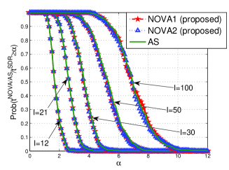
(a)

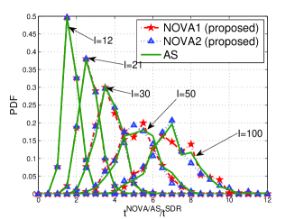
(b)

Figure 5: (a): $\text{{Prob}}(t^{\text{NOVA}/\text{AS}}/t^{\text{SDR}}\geq\alpha)$ versus $\alpha$, for $I=12,\,21,\,30,\,50,\,100$; (b): Estimated p.d.f. of $t^{\text{NOVA}}/t^{\text{SDR}}$ and $t^{\text{AS}}/t^{\text{SDR}}$.

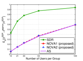
Figure 6: Average normalized distance of the achieved minimum SINR from the SDP upper bound versus $I$.

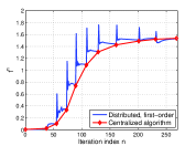
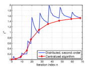
Figure 7: Minimum rate vs. iterations. Left plot: Centralized algorithm vs. Distributed, first order; Right plot: Centralized algorithm vs. Distributed, second order.

IV Concluding Remarks

In this two-part paper we introduced and analyzed a new algorithmic framework for the distributed minimization of nonconvex functions, subject to nonconvex constraints. Part I [44] developed the general framework and studied its convergence properties. In this Part II, we customized our general results to two challenging and timely problems in communications, namely: 1) the rate profile maximization in MIMO IBCs; and 2) the max-min fair multicast multigroup beamforming problem in multi-cell systems. Our algorithms i) were proved to converge to d-stationary solutions of the aforementioned problems; ii) represent the first attempt to design distributed solution methods for 1) and 2); and iii) were shown numerically to reach better local optimal solutions than ad-hoc schemes proposed in the literature for special cases of the considered formulations.

We remark that, although we considered in details only problems 1) and 2) above, the applicability of our framework goes much beyond these two specific formulations and, more generally, applications in communications. Moreover, even within the network systems considered in 1) and 2), one can consider alternative objective functions and constraints. Two examples of unsolved problems to which our framework readily applies (with convergence guarantees) are: 1) the distributed minimization of the BS’s (weighted) transmit power over MIMO IBCs, subject to rate constraints; and 2) the maximization of the (weighted) sum of the multi-cast multigroup capacity in multi-cell systems.

Our framework finds applications also in other areas, such as signal processing, smart grids, and machine learning.

-A Proof of Lemma 6

Let $\bar{\mathbf{Q}}_{i_{k}}\triangleq\mathbf{U}_{{i_{k}}}^{\nu H}\mathbf{Q}_{i_{k}}\mathbf{U}_{{i_{k}}}^{\nu}$, and $\bar{\mathbf{Q}}_{k}\triangleq(\bar{\mathbf{Q}}_{i_{k}})_{i_{k}\in\mathcal{I}_{k}}$. Then, each problem $\min_{\mathbf{Q}_{k}\in\mathcal{Q}_{k}}\mathcal{L}_{\mathbf{Q}_{k}}(\mathbf{Q}_{k},\boldsymbol{\lambda},\boldsymbol{\Omega};\mathbf{Q}^{\nu})$ in (12) can be rewritten as

$$\begin{array}[]{cl}{\displaystyle\min_{\bar{\mathbf{Q}}_{k}=(\bar{\mathbf{Q}}_{i_{k}}\succeq\mathbf{0})_{i_{k}\in\mathcal{I}_{k}}}}&{\displaystyle\sum_{i_{k}\in\mathcal{I}_{k}}}\text{tr}\left(\left(\tau_{\mathbf{Q}}\bar{\mathbf{Q}}_{i_{k}}^{H}-\mathbf{D}_{i_{k}}^{\nu}\right)\,\bar{\mathbf{Q}}_{i_{k}}\right)\\ \text{s.t.}&{\displaystyle\sum_{i_{k}\in\mathcal{I}_{k}}}\text{tr}(\bar{\mathbf{Q}}_{i_{k}})\leq P_{k}.\end{array}$$ (33)

We claim that the optimal solution of (33) must be diagonal. Indeed, denoting by $\texttt{{diag}}(\bar{\mathbf{Q}}_{i_{k}})$ the diagonal matrix having the same diagonal entries of $\bar{\mathbf{Q}}_{i_{k}}$, and $\texttt{{off}}(\bar{\mathbf{Q}}_{i_{k}})\triangleq\bar{\mathbf{Q}}_{i_{k}}-\texttt{{diag}}(\bar{\mathbf{Q}}_{i_{k}})$, (each term in the sum of) the objective function of (33) can be lower bounded as

$$\begin{array}[]{l}\text{tr}\left(\left(\tau_{\mathbf{Q}}\bar{\mathbf{Q}}_{i_{k}}^{H}-\mathbf{D}_{i_{k}}^{\nu}\right)\bar{\mathbf{Q}}_{i_{k}}\right)\vskip 6.0pt plus 2.0pt minus 2.0pt\\ \qquad=\text{tr}\left(\left(\tau_{\mathbf{Q}}\texttt{{diag}}(\bar{\mathbf{Q}}_{i_{k}})-\mathbf{D}_{i_{k}}^{\nu}\right)\texttt{{diag}}(\bar{\mathbf{Q}}_{i_{k}})\right)\vskip 3.0pt plus 1.0pt minus 1.0pt\\ \qquad\,\,\,\,\,+\text{tr}\left(\tau_{\mathbf{Q}}\texttt{{off}}(\bar{\mathbf{Q}}_{i_{k}})^{H}\texttt{{off}}(\bar{\mathbf{Q}}_{i_{k}})\right)\vskip 6.0pt plus 2.0pt minus 2.0pt\\ \qquad\geq\text{tr}\left(\left(\tau_{\mathbf{Q}}\texttt{{diag}}(\bar{\mathbf{Q}}_{i_{k}})-\mathbf{D}_{i_{k}}^{\nu}\right)\,\texttt{{diag}}(\bar{\mathbf{Q}}_{i_{k}})\right).\end{array}$$ (34)

The claim follows from the fact that the lower bound in (34) is achieved if and only if $\texttt{{off}}(\bar{\mathbf{Q}}_{i_{k}})=\mathbf{0}$ and that constraints in (33) depend only on $\texttt{{diag}}(\bar{\mathbf{Q}}_{i_{k}})$.

Setting $\bar{\mathbf{Q}}_{i_{k}}=\texttt{{Diag}}(\bar{{\mathbf{q}}}_{i_{k}})$ to be diagonal with entries the elements of $\bar{{\mathbf{q}}}_{i_{k}}\triangleq(\bar{{q}}_{i_{k},t})_{t=1}^{T_{k}}$, (33) becomes

$$\begin{array}[]{cl}{\displaystyle{\min_{\bar{{\mathbf{q}}}_{i_{k}}\geq\mathbf{0}}}}&{\displaystyle\sum_{i_{k}\in\mathcal{I}_{k}}\sum_{t=1}^{T_{k}}}\left(\tau_{\mathbf{Q}}\bar{q}_{i_{k},t}^{2}-d_{i_{k},t}^{\nu}\cdot\bar{q}_{i_{k},t}\right)\\ \mbox{s.t.}&{\displaystyle\sum_{i_{k}\in\mathcal{I}_{k}}\sum_{t=1}^{T_{k}}}\bar{q}_{i_{k},t}\leq P_{k}.\end{array}$$ (35)

Problem (35) has a closed form solution $\bar{\mathbf{q}}_{i_{k}}^{\star}$ (up to the multiplier $\xi_{k}^{\star}$), given by

$$\bar{\mathbf{q}}_{i_{k}}^{\star}=\left[\frac{\mathbf{d}_{i_{k}}^{\nu}-\xi_{k}^{\star}}{2\tau_{\mathbf{Q}}}\right]_{+},$$ (36)

where $\xi_{k}^{\star}$ needs to be chosen so that $\sum_{i_{k}\in\mathcal{I}_{k}}\mathbf{1}^{T}\bar{\mathbf{q}}_{i_{k}}^{\star}\leq P_{k}$. This can be done, e.g., using Algorithm 4, which converges in a finite number of steps.

Data: $\mathbf{d}_{k}^{\nu}\triangleq(d_{k,j}^{\nu})_{j=1}^{T_{k}\cdot I_{k}}=(\mathbf{d}_{i_{k}}^{\nu})_{i_{k}\in\mathcal{I}_{k}}$ (arranged in decreasing order).

(S.0) Set $\mathcal{J}\triangleq\{j:\,d_{k,j}^{\nu}>0\}$.

(S.1) If $\sum_{i\in\mathcal{J}}\,\frac{d_{k,j}^{\nu}}{2\tau_{\mathbf{Q}}}\leq P_{k}$: set $\xi_{k}^{\star}=0$ and STOP.

(S.2) Repeat

(a) Set $\xi_{k}^{\star}=\left[\frac{\sum_{j\in\mathcal{J}}d_{k,j}^{\nu}-2\tau_{\mathbf{Q}}P_{k}}{\left|\mathcal{J}\right|}\right]_{+};$

(b) If $\frac{d_{k,j}^{\nu}-\xi_{k}^{\star}}{2\tau_{\mathbf{Q}}}>0$, $\forall j\in\mathcal{J}$: STOP;

else  $\mathcal{J}\triangleq\mathcal{J}/\left\{j=\left|\mathcal{J}\right|\right\}$;

until $\left|\mathcal{J}\right|=1$.

Algorithm 4 Efficient computation of $\xi_{k}^{\star}$ in (36)

The optimal solution $\mathbf{Q}_{i_{k}}^{\star}$ is thus given by $\mathbf{Q}_{i_{k}}^{\star}\triangleq\mathbf{U}_{{i_{k}}}^{\nu}\texttt{{Diag}}(\bar{{\mathbf{q}}}_{i_{k}}^{\star})\mathbf{U}_{{i_{k}}}^{\nu H}$, with $\bar{{\mathbf{q}}}_{i_{k}}^{\star}$ defined in (36), which completes the proof.

-B Proof of Lemma 7

Let $\mathbf{V}_{i_{k}}^{\nu}\mathbf{D}_{i_{k}}^{\nu}\mathbf{V}_{i_{k}}^{\nu H}$ be the eigenvalue/eigenvector decomposition of $2\tau_{\mathbf{Y}}\mathbf{Y}_{i_{k}}^{\nu}-\boldsymbol{\Omega}_{i_{k}}^{\nu}$, with $\mathbf{D}_{i_{k}}^{\nu}=\texttt{{Diag}}(\mathbf{d}_{i_{k}}^{\nu})$; define $\bar{\mathbf{Y}}_{i_{k}}\triangleq\mathbf{V}_{i_{k}}^{\nu H}\mathbf{Y}_{i_{k}}\mathbf{V}_{i_{k}}^{\nu}$. Each $\min_{(\mathbf{Y}_{i_{k}}\succeq\mathbf{0})_{i_{k}\in\mathcal{I}_{k}}}\mathcal{L}_{\mathbf{Y}_{k}}(\mathbf{Y}_{k},\boldsymbol{\lambda},\boldsymbol{\Omega};\mathbf{Y}^{\nu})$ in (12) can be decomposed in $I_{k}$ separate subproblems, the $i_{k}$-th of which is

$$\begin{split}{\displaystyle\min_{\bar{\mathbf{Y}}_{i_{k}}\succeq\mathbf{0}}}\text{tr}\left(\left(\tau_{\mathbf{Y}}\bar{\mathbf{Y}}_{i_{k}}^{H}-\mathbf{D}_{i_{k}}^{\nu}\right)\,\bar{\mathbf{Y}}_{i_{k}}\right)-&\lambda_{i_{k}}^{\nu}\log\det\left(\sigma_{i_{k}}^{2}\mathbf{I}+\bar{\mathbf{Y}}_{i_{k}}\right)\end{split}.$$ (37)

We claim that the optimal solution of (37) must be diagonal. This is a consequence of the following two inequalities: Denoting by $\texttt{{diag}}(\bar{\mathbf{Y}}_{i_{k}})$ the diagonal matrix having the same diagonal entries of $\bar{\mathbf{Y}}_{i_{k}}$, and $\texttt{{off}}(\bar{\mathbf{Y}}_{i_{k}})\triangleq\bar{\mathbf{Y}}_{i_{k}}-\texttt{{diag}}(\bar{\mathbf{Y}}_{i_{k}})$, we have [note that $\texttt{{diag}}(\bar{\mathbf{Y}}_{i_{k}})\succeq\mathbf{0}$]

$$\begin{array}[]{l}\text{tr}\left(\left(\tau_{\mathbf{Y}}\bar{\mathbf{Y}}_{i_{k}}^{H}-\mathbf{D}_{i_{k}}^{\nu}\right)\bar{\mathbf{Y}}_{i_{k}}\right)\vskip 3.0pt plus 1.0pt minus 1.0pt\\ \quad\geq\text{tr}\left(\left(\tau_{\mathbf{Y}}\texttt{{diag}}(\bar{\mathbf{Y}}_{i_{k}})-\mathbf{D}_{i_{k}}^{\nu}\right)\texttt{{diag}}(\bar{\mathbf{Y}}_{i_{k}})\right),\vskip 6.0pt plus 2.0pt minus 2.0pt\\ \log\det\left(\sigma_{i_{k}}^{2}\mathbf{I}+\bar{\mathbf{Y}}_{i_{k}}\right)\leq\log\det\left(\sigma_{i_{k}}^{2}\mathbf{I}+\texttt{{diag}}(\bar{\mathbf{Y}}_{i_{k}})\right),\end{array}$$

where the first inequality has been proved in (34), while the second one is the Hadamard’s inequality. Both inequalities are satisfied with equality if and only if $\bar{\mathbf{Y}}_{i_{k}}=\texttt{{diag}}(\bar{\mathbf{Y}}_{i_{k}})$.

Replacing in (37) $\bar{\mathbf{Y}}_{i_{k}}=\texttt{{diag}}(\bar{\mathbf{Y}}_{i_{k}})\triangleq\texttt{{Diag}}(\mathbf{y}_{i_{k}})$ and checking that $\mathbf{y}_{i_{k}}$ given by (16) satisfies the KKT system of the resulting convex optimization problem, one get the closed form expression (16).

-C Augmented Hessian and Gradient Expressions in (19)

In this section, we provide the closed form expressions for the augmented Hessian matrices and gradients of the updating rules given in (19). More specifically, we have

$$\begin{split}\nabla_{\boldsymbol{\lambda},\text{vec}(\boldsymbol{\Omega}^{*})}D(\boldsymbol{\lambda},\boldsymbol{\Omega};&\mathbf{W}^{\nu})\triangleq[\nabla_{\boldsymbol{\lambda}}D(\boldsymbol{\lambda},\boldsymbol{\Omega};\mathbf{W}^{\nu});\\ &\text{vec}(\nabla_{\boldsymbol{\Omega}^{*}}D(\boldsymbol{\lambda},\boldsymbol{\Omega};\mathbf{W}^{\nu}))].\end{split}$$ (38)

Define

$$\mathbf{\bar{W}}^{n}\triangleq(R^{\star}(\boldsymbol{\lambda}^{n};R^{\nu}),\mathbf{Q}^{\star}(\boldsymbol{\lambda}^{n},\boldsymbol{\Omega}^{n};\mathbf{Q}^{\nu}),\mathbf{Y}^{\star}(\boldsymbol{\lambda}^{n},\boldsymbol{\Omega}^{n};\mathbf{Y}^{\nu}))$$

and

$$\begin{array}[]{lll}\nabla_{\lambda_{i_{k}}}D(\boldsymbol{\lambda}^{n},\boldsymbol{\Omega}^{n};\mathbf{W}^{\nu})&=&\hat{h}_{i_{k}}(\mathbf{W};\mathbf{Q}^{\nu})\mid_{\mathbf{W}=\mathbf{\bar{W}}^{n}}\vskip 6.0pt plus 2.0pt minus 2.0pt\\ \nabla_{\boldsymbol{\Omega}_{i_{k}}^{*}}D(\boldsymbol{\lambda}^{n},\boldsymbol{\Omega}^{n};\mathbf{W}^{\nu})&=&{h}_{i_{k}}(\mathbf{W})|_{\mathbf{W}=\mathbf{\bar{W}}^{n}}\end{array}$$

where

$$\begin{array}[]{lll}\hat{h}_{i_{k}}(\mathbf{W};\mathbf{Q}^{\nu})&\triangleq&\alpha_{i_{k}}{R}-\widehat{R}_{i_{k}}\left(\mathbf{Q}_{-i_{k}},\mathbf{Y}_{i_{k}};\mathbf{Q}^{\nu}\right)\vskip 6.0pt plus 2.0pt minus 2.0pt\\ {h}_{i_{k}}(\mathbf{W})&\triangleq&\mathbf{Y}_{i_{k}}-\mathbf{I}_{i_{k}}(\mathbf{Q}).\end{array}$$

Then, we have

$$\mathbf{G}\triangleq [(\text{vec}(\nabla_{\mathbf{W}^{*}}\hat{h}_{i_{k}}(\bar{\mathbf{W}}^{n};\mathbf{Q}^{\nu}))^{H})_{\forall i_{k}\in\mathcal{I}};$$ (39)

$$\,(\nabla_{\mathbf{W}^{*}}{h}_{i_{k}}(\bar{\mathbf{W}}^{n};\mathbf{Q}^{\nu}))_{\forall i_{k}\in\mathcal{I}}],$$

with

$$\begin{split}&\nabla_{\boldsymbol{\lambda},\text{vec}(\boldsymbol{\Omega}^{*})}^{2}D(\boldsymbol{\lambda}^{n},\boldsymbol{\Omega}^{n};\mathbf{W}^{\nu})=\mathbf{G}\cdot\boldsymbol{\mathcal{H}}(\bar{\mathbf{W}}^{n};\mathbf{W}^{\nu})^{-1}\cdot\mathbf{G}^{H}\end{split},$$

and

$$\boldsymbol{\mathcal{H}}(\bar{\mathbf{W}}^{n};\mathbf{W}^{\nu})=\text{bdiag}(\nabla_{\mathbf{Q}^{*}}^{2}\mathcal{L},{\displaystyle{\frac{d^{2}\mathcal{L}}{d{R}^{2}}},\nabla_{\mathbf{Y}^{*}}^{2}\mathcal{L}),}$$

where, for notation simplicity, we assume $\mathcal{L}=\mathcal{L}(\bar{\mathbf{W}}^{n},\boldsymbol{\lambda}^{n},\boldsymbol{\Omega}^{n};\mathbf{W}^{\nu})$.

It follows that

$$\begin{split}&\nabla_{\mathbf{Q}^{*}}^{2}\mathcal{L}=\text{bdiag}\left((\boldsymbol{\mathcal{H}}_{\mathbf{Q}_{j_{m}}}(\bar{\mathbf{W}}^{n},\boldsymbol{\lambda}^{n},\boldsymbol{\Omega}^{n};\mathbf{W}^{\nu}))_{j_{m}\in\mathcal{I}}\right),\\ &\nabla_{\mathbf{Y}^{*}}^{2}\mathcal{L}=\text{bdiag}\left((\boldsymbol{\mathcal{H}}_{\mathbf{Y}_{j_{m}}}(\bar{\mathbf{W}}^{n},\boldsymbol{\lambda}^{n},\boldsymbol{\Omega}^{n};\mathbf{W}^{\nu}))_{j_{m}\in\mathcal{I}}\right),\\ &{\displaystyle{\frac{d^{2}\mathcal{L}}{d{R}^{2}}}=\tau_{R},}\end{split}$$ (40)

with

$$\begin{split}&\begin{split}\boldsymbol{\mathcal{H}}_{\mathbf{Q}_{j_{m}}}(\bar{\mathbf{W}}^{n},\boldsymbol{\lambda}^{n},\boldsymbol{\Omega}^{n};\mathbf{W}^{\nu})=&2\,\tau_{\mathbf{Q}}(\mathbf{I}_{T_{k}}\otimes\mathbf{I}_{T_{k}}),\end{split}\\ &\begin{split}\boldsymbol{\mathcal{H}}_{\mathbf{Y}_{j_{m}}}(\bar{\mathbf{W}}^{n},&\boldsymbol{\lambda}^{n},\boldsymbol{\Omega}^{n};\mathbf{W}^{\nu})=2\,\tau_{\mathbf{Y}}(\mathbf{I}_{M_{i_{k}}}\otimes\mathbf{I}_{M_{i_{k}}})+\lambda_{i_{k}}^{n}\cdot\\ &\left[{(\sigma_{i_{k}}^{2}\mathbf{I}+\mathbf{Y}_{i_{k}}^{n})^{-1}}^{H}\otimes(\sigma_{i_{k}}^{2}\mathbf{I}+\mathbf{Y}_{i_{k}}^{n})^{-1}\right].\end{split}\end{split}$$ (41)

Finally, we obtain

$$\begin{array}[]{l}\text{vec}(\nabla_{\mathbf{W}^{*}}\hat{h}_{i_{k}}(\bar{\mathbf{W}}^{n};\mathbf{Q}^{\nu}))=[(\mathbf{M}_{j_{l}}^{i_{k}})_{j_{l}\in\mathcal{I}}^{H},\alpha_{i_{k}},(\mathbf{N}_{j_{l}}^{i_{k}})_{j_{l}\in\mathcal{I}}^{H}]^{H},\vskip 6.0pt plus 2.0pt minus 2.0pt\\ \nabla_{\mathbf{W}^{*}}{h}_{i_{k}}(\bar{\mathbf{W}}^{n})=[{(\mathbf{F}_{j_{l}}^{i_{k}})}_{j_{l}\in\mathcal{I}},\mathbf{0}_{M_{i_{k}}^{2}\times 1},{(\mathbf{G}_{j_{l}}^{i_{k}})}_{j_{l}\in\mathcal{I}}],\end{array}$$

where

$$\begin{split}&\mathbf{M}_{j_{l}}^{i_{k}}=\left\{\begin{array}[]{lll}(\mathbf{I}_{T_{k}}\otimes\mathbf{\Pi}_{i_{k},j_{l}}^{-})\text{vec}(\mathbf{I}_{T_{k}}),\quad\;\text{if}\;j_{l}\neq i_{k}\\ (\mathbf{0}_{T_{k}}\otimes\mathbf{0}_{T_{k}})\text{vec}(\mathbf{0}_{T_{k}}),\hskip 19.91684pt\text{otherwise;}\end{array}\right.\\ &\mathbf{N}_{j_{l}}^{i_{k}}=\left\{\begin{array}[]{lll}(\mathbf{I}_{M_{i_{k}}}\otimes(\sigma_{i_{k}}^{2}\mathbf{I}+\mathbf{Y}_{i_{k}})^{-1})\text{vec}(\mathbf{I}_{M_{i_{k}}}),\quad\;\text{if}\;j_{l}=i_{k};\\ (\mathbf{0}_{M_{i_{k}}}\otimes\mathbf{0}_{M_{i_{k}}})\text{vec}(\mathbf{0}_{M_{i_{k}}}),\hskip 58.32823pt\mbox{otherwise;}\end{array}\right.\\ &\mathbf{F}_{j_{l}}^{i_{k}}=-(\mathbf{H}_{i_{k}l}^{*}\otimes\mathbf{H}_{i_{k}l})\hskip 23.04666pt\forall j_{l}\in\mathcal{I};\\ &\mathbf{G}_{j_{l}}^{i_{k}}=\left\{\begin{array}[]{lll}(\mathbf{I}_{M_{i_{k}}}\otimes\mathbf{I}_{M_{i_{k}}}),\quad\;\text{if}\;j_{l}=i_{k};\\ (\mathbf{0}_{M_{i_{k}}}\otimes\mathbf{0}_{M_{i_{k}}}),\hskip 9.95863pt\text{otherwise}.\end{array}\right.\end{split}$$

-D Proof of Theorem 10

The proof of convergence follows readily from Proposition 9 and [3, Th.2], and thus is omitted. So does $t^{\infty}>0$, when the algorithm does not converge in a finite number of steps. Then, we only need to prove that, if $t^{0}>0$, then $\hat{t}(\boldsymbol{\lambda};t^{\nu},\boldsymbol{\beta}^{\nu})>0$, for all $\nu\geq 1$ and $\boldsymbol{\lambda}\geq 0$. Because of space limitations, we consider (29) with surrogate $\tilde{g}_{i}$ given by (26) only.

It is not difficult to see that, given the current iterate $(t^{\nu},\boldsymbol{\beta}^{\nu},\mathbf{w}^{\nu})$, $\hat{t}(\boldsymbol{\lambda};t^{\nu},\boldsymbol{\beta}^{\nu})$ has the following expression:

$$\hat{t}(\boldsymbol{\lambda};t^{\nu},\boldsymbol{\beta}^{\nu})=\frac{t^{\nu}+\tau_{t}\cdot(t^{\nu})^{2}}{\tau_{t}\cdot t^{\nu}+\boldsymbol{\lambda}^{T}\boldsymbol{\beta}^{\nu}},$$ (42)

where $\boldsymbol{\lambda}$ and $\boldsymbol{\eta}$ are the (nonnegative) multipliers associated with the constraints $\tilde{g}_{i_{k}}(t,\beta_{i_{k}},\mathbf{w}_{k};t^{\nu},\beta_{i_{k}}^{\nu},\mathbf{w}_{k}^{\nu})\leq 0$ and (b), respectively. It follows from (42), that if $t^{0}\neq 0$, then ${t}^{1}=t^{0}+\gamma^{0}(\hat{t}(\boldsymbol{\lambda};t^{0},\boldsymbol{\beta}^{0})-t^{0})>0$. Therefore, so is $t^{\nu}$, for $\nu\geq 2$.

Appendix A Supporting Material

A-A Proof of Proposition 2

(i): The proof follows readily by inspection of the MFCQ, written for Problem $\mathcal{P}_{s}$, and thus is omitted.
(ii): We prove the statement in a more general setting. Consider the following two optimization problems

$$\begin{array}[]{cl}\underset{\mathbf{x}\in\mathcal{K}}{\min}&F\left(\mathbf{x}\right)\triangleq\max\left\{f_{1}(\mathbf{x}),\cdots,f_{I}(\mathbf{x})\right\}\end{array}$$ (43)

and

$$\begin{array}[]{cl}\underset{\mathbf{x},\,t\leq 0}{\textrm{min}}&t\\ \textrm{\,\,s. t.}&f_{i}(\mathbf{x})\leq t,\ \forall i\in\mathcal{I},\\ &\mathbf{x}\in\mathcal{K},\vspace{-0.1cm}\end{array}$$ (44)

where each $f_{i}:\mathcal{K}\rightarrow\mathbb{{R}}_{-}$ is a nonpositive (possibly nonconvex) differentiable function with Lipschitz gradient on $\mathcal{K}$; $\mathcal{K}\subseteq\mathbb{{R}}^{n}$ is a (nonempty) closed and convex set (with nonempty relative interior); and $\mathcal{I}\triangleq\{1,\cdots,I\}$. We also assume that (43) has a solution.

In order to prove Proposition 2(a), it is sufficient to show the following equivalence between (43) and (44): $\mathbf{x}^{\star}$ is a d-stationary solution of (43) if and only if there exists a $t^{\star}$ such that $\left(\mathbf{x}^{\star},t^{\star}\right)$ is a regular stationary point of (44).

We first introduce some preliminary results. Denoting by $\partial F(\mathbf{x})$ the set of subgradients of $F$ at $\mathbf{x}$ (see [45, Definition 1.77]), we recall that, since each $f_{i}$ is continuously differentiable, we can write [46, Corollary 10.51]

$$\partial F(\mathbf{x})=\mathtt{con}\left(\left\{\nabla f_{i}(\mathbf{x}):\,i\in\mathcal{I}(\mathbf{x})\right\}\right),$$

where $\mathcal{I}\left(\mathbf{x}\right)\triangleq\{i\in\mathcal{I}:\,{\displaystyle F(\mathbf{x})}=f_{i}(\mathbf{x})\}$ and $\mathtt{con}(\mathcal{A})$ denotes the convex hull of the set $\mathcal{A}$. Moreover, invoking again [46, Corollary 10.51] and thanks to [46, Theorem 9.16], the directional derivative of $F^{{}^{\prime}}$ at $\mathbf{x}$ in the direction $\mathbf{d}$, $F^{\prime}(\mathbf{x};\mathbf{d})$, exists for every $\mathbf{x}\in{\mathcal{K}}$ and $\mathbf{d}\in\mathbb{R}^{n}$, and it is given by

$$F^{\prime}(\mathbf{x};\mathbf{d})=\max\left\{\left\langle\boldsymbol{\xi},\mathbf{d}\right\rangle:\boldsymbol{\xi}\in\partial F\left(\mathbf{x}\right)\right\}.$$ (45)

Using the above definitions, if $\mathbf{x}^{\star}$ is a d-stationary solution of (43), there exists $\boldsymbol{\alpha^{\star}}\in\mathbb{R}_{+}^{I}$ such that the following holds:

$$\begin{array}[]{rcl}{\displaystyle{\sum_{i\in\mathcal{I}}}\alpha_{i}^{\star}\nabla f_{i}\left(\mathbf{x}^{\star}\right)^{T}\left(\mathbf{x}-\mathbf{x}^{\star}\right)}&\geq&0,\quad\forall\mathbf{x}\in{\mathcal{K}},\\[5.0pt] {\displaystyle{\sum_{i\in{\mathcal{I}}}}\alpha_{i}^{\star}}&=&1,\\[5.0pt] \alpha_{i}^{\star}&\geq&0,\,\forall i\in\mathcal{I}\left(\mathbf{x}^{\star}\right),\\[5.0pt] \alpha_{i}^{\star}&=&0,\,\forall i\in{\mathcal{I}}\setminus\mathcal{I}\left(\mathbf{x}^{\star}\right).\end{array}$$ (46)

On the other hand, if $\left(\bar{\mathbf{x}},\bar{t}\right)$ is regular stationary for (44), there exists $\bar{\boldsymbol{\lambda}}\in\mathbb{R}_{+}^{I}$ such that

$$\begin{array}[]{rcl}{\displaystyle{\sum_{i\in\mathcal{I}}}}\bar{\lambda}_{i}\nabla f_{i}(\bar{\mathbf{x}})^{T}(\mathbf{x}-\bar{\mathbf{x}})&\geq&0,\quad\forall\mathbf{x}\in{\mathcal{K}},\\[5.0pt] 0\leq\,{\displaystyle{\sum_{i\in\mathcal{I}}}\bar{\lambda}_{i}}-1&\,\perp&\bar{t}\leq 0,\\[5.0pt] 0\leq\,\bar{\lambda}_{i}&\perp&\,f_{i}(\bar{\mathbf{x}})-\bar{t}\,\leq 0,\quad\forall i\in\mathcal{I}.\end{array}$$ (47)

We are now ready to prove the desired result.

$\left(\boldsymbol{\Rightarrow}\right)$ Let $\mathbf{x}^{\star}$ be a d-stationary point of (43). By taking $\left(\bar{\mathbf{x}},\bar{t},\bar{\boldsymbol{\lambda}}\right)\triangleq\left(\mathbf{x}^{\star},F(\mathbf{x}^{\star}),\boldsymbol{{\alpha}}^{\star}\right)$ and using (46), it is not difficult to check that the tuple $\left(\bar{\mathbf{x}},\bar{t},\bar{\boldsymbol{\lambda}}\right)$ satisfies the KKT conditions (47). Therefore $\left(\bar{\mathbf{x}},\bar{t}\right)$ is stationary for (44).

$\left(\boldsymbol{\Leftarrow}\right)$ Let $\left(\bar{\mathbf{x}},\bar{t}\right)$ be a regular stationary point of (44). Then, there exists $\bar{\boldsymbol{\lambda}}\in\mathbb{R}_{+}^{I}$ such that $\left(\bar{\mathbf{x}},\bar{t},\bar{\boldsymbol{\lambda}}\right)$ satisfies KKT conditions (47). Since ${\sum_{i\in\mathcal{I}}}\bar{\lambda}_{i}>0$, it must be $\bar{t}=f_{i_{0}}(\bar{\mathbf{x}})$, for some $i_{0}\in\mathcal{I}$. Therefore, $\bar{t}=F(\bar{\mathbf{x}})$. Furthermore, since $\mathcal{I}\left(\bar{\mathbf{x}}\right)=\left\{i\in\mathcal{I}:\,\bar{t}=f_{i}\left(\bar{\mathbf{x}}\right)\right\}$, we have $\bar{\lambda}_{j}=0$ for every $j\in{\mathcal{I}}\setminus\mathcal{I}\left(\bar{\mathbf{x}}\right)$. Define $\tilde{{\lambda}}_{i}\triangleq\bar{\lambda}_{i}/\bar{\lambda}^{\text{{ave}}}$, for all $i\in\mathcal{I}$, where $\bar{\lambda}^{\text{{ave}}}\triangleq\sum_{i\in\mathcal{I}\left(\bar{\mathbf{x}}\right)}\bar{\lambda}_{i}>0$. It follows that $\sum_{i\in\mathcal{I}\left(\bar{\mathbf{x}}\right)}\tilde{{\lambda}}_{i}=1$, and

$$\sum_{i\in\mathcal{I}}\tilde{{\lambda}}_{i}\nabla f_{i}(\bar{\mathbf{x}})=\sum_{i\in\mathcal{I}\left(\bar{\mathbf{x}}\right)}\tilde{{\lambda}}_{i}\nabla f_{i}(\bar{\mathbf{x}})\in\partial F\left(\bar{\mathbf{x}}\right).$$

Therefore, for every $\mathbf{x}\in\mathcal{K}$,

$$\begin{array}[]{rcl}F^{\prime}\left(\bar{\mathbf{x}};\mathbf{x}-\bar{\mathbf{x}}\right)&=&\max\left\{\left\langle\boldsymbol{\xi},\mathbf{x}-\bar{\mathbf{x}}\right\rangle:\boldsymbol{\xi}\in\partial F\left(\bar{\mathbf{x}}\right)\right\}\vskip 3.0pt plus 1.0pt minus 1.0pt\\ &\geq&{\displaystyle{\sum_{i\in\mathcal{I}\left(\bar{\mathbf{x}}\right)}}\tilde{{\lambda}}_{i}\nabla f_{i}(\bar{\mathbf{x}})^{T}(\mathbf{x}-\bar{\mathbf{x}})\vskip 3.0pt plus 1.0pt minus 1.0pt}\\ &=&\left(1/\bar{\lambda}^{\text{{ave}}}\right)\cdot{\displaystyle{\sum_{i\in\mathcal{I}}}\bar{\lambda}_{i}\nabla f_{i}(\bar{\mathbf{x}})^{T}(\mathbf{x}-\bar{\mathbf{x}})\geq 0,}\end{array}$$

where the last inequality follows from (47) and $\bar{\lambda}^{\text{{ave}}}>0$. Thus, $\bar{\mathbf{x}}$ is d-stationary for (43). This completes the proof of statement (ii).

A-B Proof of Proposition 9

A-B1 Preliminaries

Let us start by introducing some intermediate results needed to prove the proposition. For notation simplicity, let define $y_{i_{k}}(\mathbf{w})\triangleq\sum_{\ell\neq k}{\mathbf{w}_{\ell}^{H}\mathbf{H}_{i_{k}\ell}\mathbf{w}_{\ell}}+\sigma_{i_{k}}^{2}$, for all $i_{k}\in\mathcal{G}_{k}$ and $k\in\mathcal{K}_{\text{{BS}}}$.
Following the same arguments as in Appendix A-A [cf. (46)], if $\mathbf{w}^{\star}$ is a d-stationary solution of (21), then there exists $\boldsymbol{\alpha}^{\star}\in\mathbb{R}_{+}^{I}$ such that $(\mathbf{w}^{\star},\boldsymbol{\alpha}^{\star})$ satisfies

$$\begin{array}[]{l}(a):\,\,{\displaystyle\sum_{k\in\mathcal{K}_{\text{{BS}}}}\sum_{i_{k}\in\mathcal{G}_{k}}\alpha_{i_{k}}^{\star}\left\langle\nabla_{\mathbf{w}^{*}}u_{i_{k}}(\mathbf{w}^{\star}),\mathbf{w}-\mathbf{w}^{\star}\right\rangle}\leq 0,\,\,\,\forall\mathbf{w}\in{\mathcal{W}},\vskip 3.0pt plus 1.0pt minus 1.0pt\\ ({b)}:\,\,{\displaystyle\sum_{k\in\mathcal{K}_{\text{{BS}}}}\sum_{i_{k}\in\mathcal{G}_{k}}\alpha_{i_{k}}^{\star}}=1,\vskip 3.0pt plus 1.0pt minus 1.0pt\\ ({c)}:\,\,\alpha_{i_{k}}^{\star}\geq 0,\qquad\forall i_{k}\in\mathcal{I}\left(\mathbf{w}^{\star}\right),\vskip 3.0pt plus 1.0pt minus 1.0pt\\ ({d)}:\,\,\alpha_{i_{k}}^{\star}=0,\qquad\forall i_{k}\notin\mathcal{I}\left(\mathbf{w}^{\star}\right),\end{array}$$ (48)

where $u_{i_{k}}(\mathbf{w})\triangleq\mathbf{w}_{k}^{H}\mathbf{H}_{i_{k}k}\mathbf{w}_{k}/y_{i_{k}}(\mathbf{w})$, $\nabla_{\mathbf{w}^{*}}u_{i_{k}}(\mathbf{w})=(\nabla_{\mathbf{w}_{\ell}^{*}}u_{i_{k}}(\mathbf{w}))_{\ell\in\mathcal{K}_{\text{{BS}}}}$, with

$$\nabla_{\mathbf{w}_{\ell}^{*}}u_{i_{k}}(\mathbf{w})\triangleq\left\{\begin{array}[]{ll}\frac{1}{y_{i_{k}}(\mathbf{w})}\,\mathbf{H}_{i_{k}k}\mathbf{w}_{k},&\ \ell=k\vskip 3.0pt plus 1.0pt minus 1.0pt\\ -\frac{\mathbf{w}_{k}^{H}\mathbf{H}_{i_{k}k}\mathbf{w}_{k}}{\left(y_{i_{k}}(\mathbf{w})\right)^{2}}\,\nabla_{\mathbf{w}_{\ell}^{*}}y_{i_{k}}(\mathbf{w}),&\ \ell\neq k;\end{array}\right.$$

and $\mathcal{I}(\mathbf{w}^{\star})\!\triangleq\!\left\{i_{k}:U(\mathbf{w}^{\star})=u_{i_{k}}(\mathbf{w}^{\star})\right\}$, with $U$ defined in (21).

On the other hand, if $(\bar{{t}},\bar{{\boldsymbol{\beta}}},\bar{{\mathbf{w}}})$ is a regular stationary solution of (22), there exist multipliers $(\bar{{\boldsymbol{{\lambda}}}},\bar{{\boldsymbol{{\eta}}}},\bar{{\boldsymbol{{\rho}}}})=((\bar{{\lambda}}_{i_{k}}$, $\bar{{\eta}}_{i_{k}}$, $\bar{{\rho}}_{i_{k}})_{i_{k}\in\mathcal{G}_{k}})_{k\in\mathcal{K}_{\text{{BS}}}}$ and $\bar{{\zeta}}$ such that the following KKT conditions (referred, to be precise, to problem (22) where both sides of constraints (a) are divided by ${\beta}_{i_{k}}>0$) are satisfied

$$\!\!\!\!\!\!\!\begin{array}[]{l}(a^{{}^{\prime}}):\!\!{\displaystyle\sum_{k\in\mathcal{K}_{\text{{BS}}}}\!\sum_{i_{k}\in\mathcal{G}_{k}}}\!\!\left\langle\nabla_{\mathbf{w}^{*}}\!\!\left(\frac{\bar{{\lambda}}_{i_{k}}}{\bar{{\beta}}_{i_{k}}}\bar{{\mathbf{w}}}_{k}^{H}\mathbf{H}_{i_{k}k}\bar{{\mathbf{w}}}_{k}\!-\bar{{\eta}}_{i_{k}}\,y_{i_{k}}(\bar{{\mathbf{w}}})\right)\!,\mathbf{w}-\bar{{\mathbf{w}}}\right\rangle\vskip 3.0pt plus 1.0pt minus 1.0pt\\ \hfill\leq 0,\,\,\forall\mathbf{w}\in\mathcal{W},\\ ({b^{{}^{\prime}})}:\!\!{\displaystyle\sum_{k\in\mathcal{K}_{\text{{BS}}}}\sum_{i_{k}\in\mathcal{G}_{k}}}\bar{{\lambda}}_{i_{k}}=1+\bar{{\zeta}},\vskip 3.0pt plus 1.0pt minus 1.0pt\\ ({c^{{}^{\prime}})}:\,\,\bar{\eta}_{i_{k}}={\displaystyle{\frac{\bar{{\lambda}}_{i_{k}}\bar{{\mathbf{w}}}_{k}^{H}\mathbf{H}_{i_{k}k}\bar{{\mathbf{w}}}_{k}}{\bar{{\beta}}_{i_{k}}^{2}}}+\bar{{\rho}}_{i_{k}},\qquad\quad\;\forall i_{k}\in\mathcal{G}_{k},k\in\mathcal{K}_{\text{{BS}}},\vskip 3.0pt plus 1.0pt minus 1.0pt}\\ ({d^{{}^{\prime}})}:\,\,0\leq\bar{{\lambda}}_{i_{k}}\perp\Big{(}\bar{{t}}-{\displaystyle{\frac{\bar{{\mathbf{w}}}_{k}^{H}\mathbf{H}_{i_{k}k}\bar{{\mathbf{w}}}_{k}}{\bar{{\beta}}_{i_{k}}}}\Big{)}\leq 0,\;\,\,\forall i_{k}\in\mathcal{G}_{k},k\in\mathcal{K}_{\text{{BS}}},\vskip 3.0pt plus 1.0pt minus 1.0pt}\\ ({e^{{}^{\prime}})}:\,\,0\leq\bar{{\eta}}_{i_{k}}\perp{(y_{i_{k}}(\bar{{\mathbf{w}}})-\bar{{\beta}}_{i_{k}})}\leq 0,\hskip 25.6073pt\forall i_{k}\in\mathcal{G}_{k},k\in\mathcal{K}_{\text{{BS}}},\vskip 3.0pt plus 1.0pt minus 1.0pt\\ ({f^{{}^{\prime}})}:\,\,0\leq\bar{{\rho}}_{i_{k}}\perp(\bar{{\beta}}_{i_{k}}-\beta_{i_{k}}^{\max})\leq 0,\hskip 31.2982pt\forall i_{k}\in\mathcal{G}_{k},k\in\mathcal{K}_{\text{{BS}}},\vskip 3.0pt plus 1.0pt minus 1.0pt\\ ({g^{{}^{\prime}})}:\,\,0\leq\bar{{\zeta}}\perp\bar{{t}}\geq 0,\end{array}$$ (49)

where, with a slight abuse of notation, we denoted by $\nabla_{\mathbf{w}^{*}}(\bar{{\mathbf{w}}}_{k}^{H}\mathbf{H}_{i_{k}k}\bar{{\mathbf{w}}}_{k})$ and $\nabla_{\mathbf{w}^{*}}(y_{i_{k}}(\bar{{\mathbf{w}}}))$ the conjugate gradient of ${\mathbf{w}}_{k}^{H}\mathbf{H}_{i_{k}k}\mathbf{w}_{k}$ and $y_{i_{k}}(\mathbf{w})$, respectively, evaluated at $\mathbf{w}=\bar{{\mathbf{w}}}$.

Note that it must always be $\bar{{\boldsymbol{{\rho}}}}=\mathbf{0}$, as shown next. Suppose that there exists a $i_{k}$ such that $\bar{{\rho}}_{i_{k}}>0$. Then, invoking the complementarity condition in $(f^{{}^{\prime}})$, we have $\bar{{\beta}}_{i_{k}}=\beta_{i_{k}}^{\max}$. Also, by the definition of $\beta_{i_{k}}^{\max}$, it must be $\bar{{\beta}}_{i_{k}}>{y_{i_{k}}(\bar{\mathbf{w}})}>0$, and thus $\bar{{\eta}}_{i_{k}}=0$ [by complementarity in $(e^{{}^{\prime}})$]. It follows from $(c^{{}^{\prime}})$ that $-\bar{{\rho}}_{i_{k}}=\bar{{\lambda}}_{i_{k}}\bar{{\mathbf{w}}}_{k}^{H}\mathbf{H}_{i_{k}k}\bar{{\mathbf{w}}}_{k}/\bar{{\beta}}_{i_{k}}^{2}<0$, which contradicts the fact that $\bar{{\lambda}}_{i_{k}}\bar{{\mathbf{w}}}_{k}^{H}\mathbf{H}_{i_{k}k}\bar{{\mathbf{w}}}_{k}/\bar{{\beta}}_{i_{k}}^{2}\geq 0$ (recall that $\mathbf{H}_{i_{k}k}$ is a positive semidefinite matrix).

A-B2 Proof of Proposition 9

We prove only statement (ii).

$(\Rightarrow)$: Let ${\mathbf{w}}^{\star}$ be a d-stationary solution of (21). Partition the set of users $\mathcal{I}$ according to $\mathcal{I}=\mathcal{I}_{\text{{a}}}(\mathbf{w}^{\star})\cup\overline{{\mathcal{I}}}_{\text{{a}}}(\mathbf{w}^{\star})$, where $\mathcal{I}_{\text{{a}}}(\mathbf{w}^{\star})$ is the set of active users at $\mathbf{w}^{\star}$ (i.e., the users served by a BS), defined as

$$\mathcal{I}_{\text{{a}}}(\mathbf{w}^{\star})\triangleq\left\{i_{k}\,:\,\mathbf{H}_{i_{k}k}\mathbf{w}_{k}^{\star}\neq\mathbf{0}\right\},$$ (50)

and $\overline{{\mathcal{I}}}_{\text{{a}}}(\mathbf{w}^{\star})$ is its complement. Note that, since all $\mathbf{H}_{i_{k}k}$ are nonzero and positive semidefinite, there must exists a feasible $\mathbf{w}=(\mathbf{w}_{k})_{k\in\mathcal{K}_{\text{{BS}}}}$ such that $\mathbf{H}_{i_{k}k}\mathbf{w}_{k}\neq\mathbf{0}$ for some $i_{k}\in\mathcal{G}_{k}$ and $k\in\mathcal{{K}}_{\text{{BS}}}$. We distinguish the following two complementary cases: either 1) $\overline{{\mathcal{I}}}_{\text{{a}}}(\mathbf{w}^{\star})\neq\emptyset$; or 2) $\overline{{\mathcal{I}}}_{\text{{a}}}(\mathbf{w}^{\star})=\emptyset$. The former is a degenerate (undesired) case: the d-stationary point $\mathbf{w}^{\star}$ is a global minimizer of $U$, since $U(\mathbf{w}^{\star})=0$. The latter case, implying $U(\mathbf{w}^{\star})>0$, is instead the interesting one, which the global optimal solution of (21) belongs to.

Case 1: $\overline{{\mathcal{I}}}_{\text{{a}}}(\mathbf{w}^{\star})\neq\emptyset$. Choose $(\bar{t},\bar{\boldsymbol{\beta}},\bar{\mathbf{w}},\bar{\boldsymbol{\lambda}},\bar{\boldsymbol{\eta}},\bar{\boldsymbol{\rho}},\bar{\zeta})$ as follows: $\bar{{t}}=0$; $\bar{\boldsymbol{\beta}}$ is any vector $\bar{\boldsymbol{\beta}}\triangleq((\bar{\beta}_{i_{k}})_{i_{k}\in\mathcal{G}_{k}})_{k\in\mathcal{K}_{\text{{BS}}}}$ satisfying the feasibility conditions in ($e^{{}^{\prime}}$) and ($f^{{}^{\prime}}$), that is, $y_{i_{k}}(\mathbf{w}^{\star})\leq\bar{\beta}_{i_{k}}\leq\beta_{i_{k}}^{\max}$, for all $i_{k}\in\mathcal{G}_{k}$ and $k\in\mathcal{K}_{\text{{BS}}}$; $\bar{\mathbf{w}}=\mathbf{w}^{\star}$; $\bar{\boldsymbol{\lambda}}=((\alpha_{i_{k}}^{\star})_{i_{k}\in\mathcal{G}_{k}})_{k\in\mathcal{K}_{\text{{BS}}}}$, $\bar{\boldsymbol{\eta}}=\bar{\boldsymbol{\rho}}=\mathbf{0}$; and $\bar{\zeta}=0$. We show next that such a tuple satisfies the KKT conditions (49).

Observe preliminary that $u_{i_{k}}(\mathbf{w}^{\star})=0$ if and only if $i_{k}\in\overline{{\mathcal{I}}}_{\text{{a}}}(\mathbf{w}^{\star})$, implying $U(\mathbf{w}^{\star})=u_{i_{k}}(\mathbf{w}^{\star})=0$, for all $i_{k}\in\overline{{\mathcal{I}}}_{\text{{a}}}(\mathbf{w}^{\star})$ [recall that all $u_{i_{k}}(\mathbf{w}^{\star})\geq 0$]; therefore, it must be

$${\mathcal{I}}(\mathbf{w}^{\star})\equiv\overline{{\mathcal{I}}}_{\text{{a}}}(\mathbf{w}^{\star}).$$ (51)

Invoking now ($d$) in (48) and using (51), we have $\bar{{\lambda}}_{i_{k}}=0$, for all $i_{k}\in{\mathcal{I}}_{\text{{a}}}(\mathbf{w}^{\star})$. It follows that

$$\bar{{\lambda}}_{i_{k}}\cdot\nabla_{\mathbf{w}^{*}}\left(\bar{{\mathbf{w}}}_{k}^{H}\mathbf{H}_{i_{k}k}\bar{{\mathbf{w}}}_{k}\right)=\mathbf{0},\quad\forall i_{k}\in\mathcal{G}_{i_{k}},\,\forall k\in\mathcal{K}_{\text{{BS}}},$$

which, together with $\bar{\boldsymbol{\eta}}=\mathbf{0}$, make ($a^{{}^{\prime}}$) in (49) satisfied, with the LHS equal to zero.

Condition ($b^{{}^{\prime}}$) follows readily from $\sum_{k\in\mathcal{K}_{\text{{BS}}}}\sum_{i_{k}\in\mathcal{G}_{k}}\bar{{\lambda}}_{i_{k}}=1$ [cf. ($b$) in (48)] and $\bar{\zeta}=0$.

Condition ($c^{{}^{\prime}}$) can be checked observing that $\bar{{\lambda}}_{i_{k}}\cdot\bar{{\mathbf{w}}}_{k}^{H}\mathbf{H}_{i_{k}k}\bar{{\mathbf{w}}}_{k}=\mathbf{0}$, for all $i_{k}\in\mathcal{G}_{i_{k}}$ and $k\in\mathcal{K}_{\text{{BS}}}$.

Conditions ($d^{{}^{\prime}}$)-($g^{{}^{\prime}}$) follow readily by inspection.

Case 2: $\overline{{\mathcal{I}}}_{\text{{a}}}(\mathbf{w}^{\star})=\emptyset$. Choose now $(\bar{t},\bar{\boldsymbol{\beta}},\bar{\mathbf{w}},\bar{\boldsymbol{\lambda}},\bar{\boldsymbol{\eta}},\bar{\boldsymbol{\rho}},\bar{\zeta})$ as follows: $\bar{{t}}=U(\mathbf{w}^{\star})$; $\bar{\boldsymbol{\beta}}=(y_{i_{k}}(\mathbf{w}^{\star}))_{i_{k}\in\mathcal{G}_{k},k\in\mathcal{K}_{\text{{BS}}}}$; $\bar{\mathbf{w}}=\mathbf{w}^{\star}$; $\bar{\boldsymbol{\lambda}}=((\alpha_{i_{k}}^{\star})_{i_{k}\in\mathcal{G}_{k}})_{k\in\mathcal{K}_{\text{{BS}}}}$; $\bar{\boldsymbol{\eta}}\triangleq(\bar{\eta}_{i_{k}})_{i_{k}\in\mathcal{G}_{k},k\in\mathcal{K}_{\text{{BS}}}}$, with each $\bar{\eta}_{i_{k}}=\bar{\lambda}_{i_{k}}\cdot u_{i_{k}}(\mathbf{w}^{\star})/y_{i_{k}}(\mathbf{w}^{\star})$; $\bar{\boldsymbol{\rho}}=\mathbf{0}$; and $\bar{\zeta}=0$.

By substitution, one can see that

$$\begin{array}[]{l}{\displaystyle\sum_{k\in\mathcal{K}_{\text{{BS}}}}\sum_{i_{k}\in\mathcal{G}_{k}}}\!\!\left\langle\nabla_{\mathbf{w}^{*}}\left(\frac{\bar{{\lambda}}_{i_{k}}}{\bar{{\beta}}_{i_{k}}}\bar{{\mathbf{w}}}_{k}^{H}\mathbf{H}_{i_{k}k}\bar{{\mathbf{w}}}_{k}\!-\bar{{\eta}}_{i_{k}}\,y_{i_{k}}(\bar{{\mathbf{w}}})\right),\mathbf{w}-\bar{{\mathbf{w}}}\right\rangle\\ ={\displaystyle\sum_{k\in\mathcal{K}_{\text{{BS}}}}\sum_{i_{k}\in\mathcal{G}_{k}}}\alpha_{i_{k}}^{\star}\left\langle\nabla_{\mathbf{w}^{*}}u_{i_{k}}(\mathbf{w}^{\star}),\mathbf{w}-\bar{{\mathbf{w}}}\right\rangle\leq 0,\,\,\forall\mathbf{w}\in\mathcal{W},\end{array}$$

where the last implication follows from ($a$) in (48); therefore, ($a^{{}^{\prime}}$) in (49) is satisfied.

Condition ($b^{{}^{\prime}}$) follows readily from $\sum_{k\in\mathcal{K}_{\text{{BS}}}}\sum_{i_{k}\in\mathcal{G}_{k}}\bar{{\lambda}}_{i_{k}}=1$ [cf. ($b$) in (48)] and $\bar{\zeta}=0$.

Condition ($c^{{}^{\prime}}$) follows by inspection.

Condition ($d^{{}^{\prime}}$) can be checked as follows. Since by ($b^{{}^{\prime}}$) there exists a $\bar{{\lambda}}_{i_{k}}>0$, it must be $\bar{{t}}={\displaystyle\bar{{\mathbf{w}}}_{k}^{H}\mathbf{H}_{i_{k}k}\bar{{\mathbf{w}}}_{k}/\bar{{\beta}}_{i_{k}},}$ which together with $\bar{{\beta}}_{i_{k}}=y_{i_{k}}(\mathbf{w}^{\star})$, can be rewritten as $\bar{{t}}=U(\mathbf{w}^{\star})$.

Finally, conditions ($e^{{}^{\prime}}$)-($g^{{}^{\prime}}$) follow by inspection.

(a) $(\Leftarrow)$: Let us prove now the converse. Let $(\bar{t},\bar{\boldsymbol{\beta}},\bar{\mathbf{w}})$ be a regular stationary point of (22). One can show that, if $\overline{{\mathcal{I}}}_{\text{{a}}}(\bar{\mathbf{w}})\neq\emptyset$, $\bar{\mathbf{w}}$ is a d-stationary solution of (21) with $U^{\prime}(\bar{\mathbf{w}};\mathbf{w}-\bar{\mathbf{w}})=0$, for all $\mathbf{w}\in\mathcal{W}$; we omit further details.

Let us consider now the nondegenerate case $\overline{{\mathcal{I}}}_{\text{{a}}}(\bar{\mathbf{w}})=\emptyset$. Let $(\bar{\boldsymbol{\lambda}},\bar{\boldsymbol{\eta}},\bar{\boldsymbol{\rho}},\bar{\zeta})$ be the multipliers such that $(\bar{t},\bar{\boldsymbol{\beta}},\bar{\mathbf{w}},\bar{\boldsymbol{\lambda}},\bar{\boldsymbol{\eta}},\bar{\boldsymbol{\rho}},\bar{\zeta})$ satisfies (49). It follows from $(b^{{}^{\prime}})$ that there exists a $\bar{\lambda}_{i_{k}}>0$. Then, we have the following chain of implication (each of them due to the condition reported on top of the implication)

$$\begin{array}[]{lll}\bar{\lambda}_{i_{k}}>0&\stackrel{{\scriptstyle(d^{{}^{\prime}})}}{{\Rightarrow}}&\bar{t}={\frac{\bar{{\mathbf{w}}}_{k}^{H}\mathbf{H}_{i_{k}k}\bar{{\mathbf{w}}}_{k}}{\bar{{\beta}}_{i_{k}}}}>0\\ &\stackrel{{\scriptstyle(c^{{}^{\prime}})}}{{\Rightarrow}}&\bar{\eta}_{i_{k}}>0\\ &\stackrel{{\scriptstyle(e^{{}^{\prime}})}}{{\Rightarrow}}&\bar{{\beta}}_{i_{k}}=y_{i_{k}}(\bar{\mathbf{w}})>0\\ &\stackrel{{\scriptstyle(d^{{}^{\prime}})}}{{\Rightarrow}}&\bar{t}=u_{i_{k}}(\bar{{\mathbf{w}}}).\end{array}$$ (52)

Denoting by $\mathcal{I}(\bar{\mathbf{w}})\triangleq\left\{i_{k}\,:\,\bar{t}=u_{i_{k}}(\bar{\mathbf{w}})\right\}$ and $\alpha_{i_{k}}^{\star}\triangleq\frac{\bar{\lambda}_{i_{k}}}{1+\bar{\zeta}},$ for all $i_{k}\in\mathcal{G}_{k}$ and $k\in\mathcal{K}_{{BS}}$, it follows from (52) and ($b^{{}^{\prime}}$) that

$$\begin{array}[]{l}\sum_{k\in\mathcal{K}_{{BS}}}\sum_{i_{k}\in\mathcal{G}_{k}}\alpha_{i_{k}}^{\star}=1,\vskip 3.0pt plus 1.0pt minus 1.0pt\\ \alpha_{i_{k}}^{\star}\geq 0,\quad\forall i_{k}\in\mathcal{I}(\bar{{\mathbf{w}}}),\vskip 3.0pt plus 1.0pt minus 1.0pt\\ \alpha_{i_{k}}^{\star}=0,\quad\forall i_{k}\notin\mathcal{I}(\bar{{\mathbf{w}}}).\end{array}$$ (53)

Using (53), we finally have

$$\begin{array}[]{c}\sum_{k\in\mathcal{K}_{{BS}}}\sum_{i_{k}\in\mathcal{G}_{k}}\alpha_{i_{k}}^{\star}\nabla_{\mathbf{w}^{*}}\left(-u_{i_{k}}(\bar{\mathbf{w}})\right)\hfill\vskip 3.0pt plus 1.0pt minus 1.0pt\\ =-\sum_{i_{k}\in\mathcal{I}(\bar{\mathbf{w}})}\alpha_{i_{k}}^{\star}\nabla_{\mathbf{w}^{*}}u_{i_{k}}(\bar{\mathbf{w}})\in\partial(-U(\bar{\mathbf{w}})),\end{array}$$

where $\partial(-U(\bar{\mathbf{w}}))$ is the set of (conjugate) subgradients of $-U$ at $\bar{\mathbf{w}}$. For every $\mathbf{w}\in\mathcal{W}$,

$$\begin{array}[]{l}-U^{\prime}(\bar{\mathbf{w}};\mathbf{w}-\bar{\mathbf{w}})=\max\left\{\left\langle\boldsymbol{\xi},\mathbf{w}-\bar{\mathbf{w}}\right\rangle:\boldsymbol{\xi}\in\partial(-U(\bar{\mathbf{w}}))\right\}\\ \geq\left\langle-\sum_{i_{k}\in\mathcal{I}(\bar{\mathbf{w}})}\alpha_{i_{k}}^{\star}\nabla_{\mathbf{w}^{*}}u_{i_{k}}(\bar{\mathbf{w}}),\mathbf{w}-\bar{\mathbf{w}}\right\rangle\\ =-\dfrac{1}{1+\bar{\zeta}}\\ \cdot{\displaystyle\sum_{k\in\mathcal{K}_{\text{{BS}}}}\sum_{i_{k}\in\mathcal{G}_{k}}}\!\!\left\langle\nabla_{\mathbf{w}^{*}}\left(\frac{\bar{{\lambda}}_{i_{k}}}{\bar{{\beta}}_{i_{k}}}\bar{{\mathbf{w}}}_{k}^{H}\mathbf{H}_{i_{k}k}\bar{{\mathbf{w}}}_{k}\!-\bar{{\eta}}_{i_{k}}\,y_{i_{k}}(\bar{{\mathbf{w}}})\right),\mathbf{w}-\bar{\mathbf{w}}\right\rangle\\ \geq 0,\end{array}$$

where the last inequality is due to $(a^{{}^{\prime}})$. This proves that $\bar{\mathbf{w}}$ is d-stationary for (21).

References

- [1] G. Scutari, F. Facchinei, L. Lampariello, and P. Song, “Parallel and distributed methods for nonconvex optimization,” in Proc. of IEEE International Conference on Acoustics, Speech, and Signal Processing (ICASSP 14), Florence, Italy, May 4-9 2014.
- [2] P. Song, G. Scutari, F. Facchinei, and L. Lampariello, “D3m: Distributed multi-cell multigroup multicasting,” in Proc. of IEEE International Conference on Acoustics, Speech, and Signal Processing (ICASSP 16), Shangai, China, March 20-25 2016.
- [3] G. Scutari, F. Facchinei, L. Lampariello, and P. Song, “Parallel and distributed methods for nonconvex optimizationPart I: Theory,” IEEE Trans. Signal Process., (submitted). [Online]. Available: arXiv:1410.4754
- [4] K. T. Phan, S. A. Vorobyov, C. Telambura, and T. Le-Ngoc, “Power control for wireless cellular systems via D.C. programming,” in IEEE/SP 14th Workshop on Statistical Signal Processing, 2007, pp. 507–511.
- [5] H. Al-Shatri and T. Weber, “Achieving the maximum sum rate using D.C. programming in cellular networks,” IEEE Trans. Signal Process., vol. 60, no. 3, pp. 1331–1341, Mar. 2012.
- [6] N. Vucic, S. Shi, and M. Schubert, “DC programming approach for resource allocation in wireless networks,” in 8th International Symposium on Modeling and Optimization in Mobile, Ad Hoc and Wireless Networks (WiOpt), 2010, pp. 380–386.
- [7] M. Chiang, C. W. Tan, D. P. Palomar, D. O. Neill, and D. Julian, “Power control by geometric programming,” IEEE Trans. Wireless Commun., vol. 6, no. 7, pp. 2640–2651, Jul. 2007.
- [8] A. Khabbazibasmenj, F. Roemer, S. A. Vorobyov, and M. Haardt, “Sum-rate maximization in two-way AF MIMO relaying: Polynomial time solutions to a class of DC programming problems,” IEEE Trans. Signal Process., vol. 60, no. 10, pp. 5478–5493, 2012.
- [9] Y. Xu, T. Le-Ngoc, and S. Panigrahi, “Global concave minimization for optimal spectrum balancing in multi-user DSL networks,” IEEE Trans. Signal Process., vol. 56, no. 7, pp. 2875–2885, Jul. 2008.
- [10] R. Cendrillon, J. Huang, M. Chiang, and M. Moonen, “Autonomous spectrum balancing for digital subscriber lines,” IEEE Trans. Signal Process., vol. 55, no. 8, pp. 4241–4257, Aug. 2007.
- [11] D. Schmidt, C. Shi, R. Berry, M. Honig, and W. Utschick, “Distributed resource allocation schemes: Pricing algorithms for power control and beamformer design in interference networks,” IEEE Signal Process. Mag., vol. 26, no. 5, pp. 53–63, Sept. 2009.
- [12] S.-J. Kim and G. B. Giannakis, “Optimal resource allocation for MIMO ad hoc cognitive radio networks,” IEEE Trans. on Information Theory, vol. 57, no. 5, pp. 3117–3131, May 2011.
- [13] G. Scutari, F. Facchinei, P. Song, D. P. Palomar, and J.-S. Pang, “Decomposition by partial linearization: Parallel optimization of multi-agent systems,” IEEE Trans. Signal Process., vol. 62, no. 3, pp. 641–656, Feb. 2014. [Online]. Available: http://arxiv.org/abs/1302.0756.
- [14] R. Zhang and S. Cui, “Cooperative interference management with miso beamforming,” IEEE Trans. Signal Process., vol. 58, no. 18, pp. 5450–5458, Oct. 2010.
- [15] R. Mochaourab, P. Cao, and E. Jorswieck, “Alternating rate profile optimization in single stream mimo interference channels,” IEEE Signal Process. Lett., no. 21, Feb. 2014.
- [16] J. Qiu, R. Zhang, Z.-Q. Luo, and S. Cui, “Optimal distributed beamforming for miso interference channels,” IEEE Trans. Signal Process., vol. 59, no. 11, pp. 5638–5643, Nov. 2011.
- [17] L. Liu, R. Zhang, and K.-C. Chua, “Achieving global optimality for weighted sum-rate maximization in the k-user gaussian interference channel with multiple antennas,” IEEE Trans. Wireless Commun., vol. 11, no. 5, pp. 1933–1945, May 2012.
- [18] M. Razaviyayn, M. Hong, and Z.-Q. Luo, “Linear transceiver design for a mimo interfering broadcast channel achieving max-min fairness,” Signal Processing, vol. 93, pp. 3327–3340, Dec. 2013.
- [19] Y. Zhang, E. Dall’Anese, and G. B. Giannakis, “Distributed optimal beamformers for cognitive radios robust to channel uncertainties,” IEEE Trans. Signal Process., vol. 60, no. 12, pp. 6495–6508, Dec. 2012.
- [20] Y. Yang, G. Scutari, P. Song, and D. P. Palomar, “Robust mimo cognitive radio systems under interference temperature constraints,” IEEE J. Sel. Areas Commun., vol. 31, no. 11, pp. 2465–2482, Nov. 2013.
- [21] F. Wang, M. Krunz, and S. Cui, “Price-based spectrum management in cognitive radio networks,” IEEE J. Sel. Topics Signal Process., vol. 2, no. 1, pp. 74–87, Feb. 2008.
- [22] E. Karipidis, N. D. Sidiropoulos, and Z.-Q. Luo, “Quality of service and max-min fair transmit beamforming to multiple cochannel multicast groups,” IEEE Trans. on Signal Process., vol. 56, no. 3, pp. 1268 – 1279, Mar. 2008.
- [23] D. Christopoulos, S. Chatzinotas, and B. Ottersten, “Weighted fair multicast multigroup beamforming under per-antenna power constraints,” IEEE Trans. on Signal Process., vol. 62, no. 19, pp. 5132 – 5142, Oct. 2014.
- [24] G.-W. Hsu, H.-H. Wang, H.-J. Su, and P. Lin, “Joint beamforming for multicell multigroup multicast with per-cell power constraints,” in 2014 IEEE 25th Annual Int. Symposium on Personal, Indoor, and Mobile Radio Communication (PIMRC), Washington, DC, Sept. 2-5 2014, pp. 527 – 532.
- [25] Z. Xiang, M. Tao, and X. Wang, “Coordinated multicast beamforming in multicell networks,” IEEE Trans. on Wireless Commun., vol. 12, no. 1, pp. 12 – 21, Jan. 2013.
- [26] M. Chiang, S. H. Low, A. R. Calderbank, and J. C. Doyle, “Layering as optimization decomposition: A mathematical theory of network architectures,” Proc. IEEE, vol. 95, no. 1, pp. 255–312, Jan. 2007.
- [27] M. Chiang, P. Hande, T. Lan, and C. W. Tan, Power control in wireless cellular networks. Foundations and Trends in Networking, Now Publishers, Jul. 2008, vol. 2, no. 4.
- [28] D. P. Palomar and M. Chiang, “Alternative distributed algorithms for network utility maximization: Framework and applications,” IEEE Trans. on Automatic Control, vol. 52, no. 12, pp. 2254–2269, Dec. 2007.
- [29] S. N. D., D. T. N., and Z.-Q. Luo, “Transmit beamforming for physical-layer multicasting,” IEEE Trans. on Signal Process., vol. 54, no. 6, pp. 2239–2251, Jun. 2006.
- [30] H. Shen, B. Li, M. Tao, and X. Wang, “Mse-based transceiver designs for the mimo interference channel,” IEEE Trans. Wireless Commun., vol. 9, no. 11, pp. 3480–3489, Sept. 2010.
- [31] C.-E. Chen and W.-H. Chung, “An iterative minmax per-stream mse transceiver design for mimo interference channel,” IEEE Wireless Commun. Lett., vol. 1, no. 3, pp. 229–232, Apr. 2012.
- [32] J. Qiu, R. Zhang, Z.-Q. Luo, and S. Cui, “Optimal distributed beamforming for miso interference channels,” IEEE Trans. Signal Process., vol. 59, no. 11, pp. 5638–5643, Jul. 2011.
- [33] D. W. H. Cai, T. Q. S. Quek, and C. W. Tan, “A unified analysis of max-min weighted sinr for mimo downlink system,” IEEE Trans. on Signal Process., vol. 59, pp. 3850–3862, Aug. 2011.
- [34] G. Scutari, F. Facchieni, J.-S. Pang, and D. P. Palomar, “Real and complex monotone communication games,” IEEE Trans. on Information Theory, vol. 60, no. 7, pp. 4197–4231, July 2014.
- [35] Q. Shi, M. Razaviyayn, Z.-Q. Luo, and C. He, “An iteratively weighted MMSE approach to distributed sum-utility maximization for a MIMO interfering broadcast channel,” IEEE Trans. Signal Process., vol. 59, no. 9, pp. 4331–4340, Sept. 2011.
- [36] B. Gopalakrishnan and N. D. Sidiropoulos, “High performance adaptive algorithms for single-group multicast beamforming,” IEEE Trans. on Signal Process., vol. 63, no. 16, pp. 4373–4384, Aug. 2015.
- [37] E. Karipidis, N. D. Sidiropoulos, and Z.-Q. Luo, “Far-field multicast beamforming for uniform linear antenna arrays,” IEEE Trans. on Signal Process., vol. 55, no. 10, pp. 4916–4927, Oct. 2007.
- [38] G. Dartmann and G. Ascheid, “Equivalent quasi-convex form of the multicast max-min beamforming problem,” IEEE Trans. on Vehicular Technology, vol. 62, no. 9, pp. 4643–4648, Nov. 2013.
- [39] Z.-Q. Luo, W.-K. Ma, A. M.-C. So, Y. Ye, and S. Zhang, “Semidefinite relaxation of quadratic optimization problems,” IEEE Signal Process. Mag., vol. 27, no. 3, pp. 20–34, May 2010.
- [40] T.-H. Chang, Z.-Q. Luo, and C.-Y. Chi, “Approximation bounds for semidefinite relaxation of max-min-fair multicast transmit beamforming problem,” IEEE Trans. on Signal Process., vol. 56, no. 8, pp. 3932–3943, Aug. 2008.
- [41] A. Schad and M. Pesavento, “Max-min fair transmit beamforming for multi-group multicasting,” in 2012 International ITG Workshop on Smart Antennas (WSA), Dresden, Germany, Mar. 7-8 2012, pp. 115 – 118.
- [42] D. Christopoulos, S. Chatzinotas, and B. Ottersten, “Multicast multigroup beamforming for per-antenna power constrained large-scale arrays,” arXiv preprint, Mar. 2015.
- [43] O. Mehanna, K. Huang, B. Gopalakrishnan, A. Konar, and N. D. Sidiropoulos, “Feasible point pursuit and successive approximation of non-convex qcqps,” IEEE Signal Process. Lett., vol. 22, no. 7, pp. 804–808, Jul. 2015.
- [44] E. Larsson, E. Jorswieck, J. Lindblom, and R. Mochaourab, “Game theory and the flat-fading gaussian interference channel,” IEEE Signal Process. Mag., vol. 26, no. 5, pp. 18–27, Sept. 2009.
- [45] B. S. Mordukhovich, Variational Analysis and Generalized Differentiation: Basic Theory. Springer, 2006.
- [46] R. Rockafellar and J. Wets, Variational Analysis. Springer, 1998.