Long tail distributions near the many body localization transition

Abstract

The random field $S=\frac{1}{2}$ Heisenberg chain exhibits a dynamical many body localization transition at a critical disorder strength, which depends on the energy density. At weak disorder, the eigenstate thermalization hypothesis (ETH) is fulfilled on average, making local observables smooth functions of energy, whose eigenstate-to-eigenstate fluctuations decrease exponentially with system size.

We demonstrate the validity of ETH in the thermal phase as well as its breakdown in the localized phase and show that rare states exist which do not strictly follow ETH, becoming more frequent closer to the transition. Similarly, the probability distribution of the entanglement entropy at intermediate disorder develops long tails all the way down to zero entanglement. We propose that these low entanglement tails stem from localized regions at the subsystem boundaries which were recently discussed as a possible mechanism for subdiffusive transport in the ergodic phase.

I Introduction

The eigenstate thermalization hypothesis (ETH)Deutsch (1991); Srednicki (1994); D’Alessio et al. (2015) is a mechanism for the thermalization of generic closed quantum systems that has been numerically verified in many models Rigol et al. (2008); Rigol (2009); Beugeling et al. (2014); Steinigeweg et al. (2013) and is also argued to be valid for typical states of integrable systems, where the approach to the thermodynamic limit is dramatically slowerAlba (2015). If it is fulfilled, it ensures that the infinite time limit of local observables of any initial state will be equal to the canonical expectation value at a temperature that is fixed by the energy of the initial state, implying that eigenstates whose energies are close to each other have very similar properties and local operators yield identical results in the thermodynamic limit. Consequently, for very large systems, local observables vary smoothly with energy and microcanonical averages are well defined, corresponding to the canonical expectation values. In systems of finite size, local observables from eigenstates in a microcanonical energy window are distributed according to a normal distribution with a variance that decreases as the square root of the dimension of the Hilbert spaceIkeda et al. (2011); Rigol and Srednicki (2012); Beugeling et al. (2014); Ikeda and Ueda (2015), due to the exponentially growing density of states with system size.

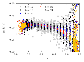
Figure 1: Local magnetization for site 5 in the chain as a function of energy. Here, we have generated one disorder configuration at $h=1.0$ for the largest system size $L_{\text{max}}=24$, smaller systems are cut out of this configuration for comparable results. The spread of the results in the middle of the spectrum reduces significantly with system size, thus leading to a smooth function of energy in the thermodynamic limit. Clearly, at the high end of the spectrum, this is no longer true and the variance of the local magnetization does not reduce with system size. This is a signal for many body localization, which is expected at $\epsilon\gtrsim 0.9$ at $h=1$ in accord with Ref. Luitz et al., 2015 and thus shows the many body mobility edge

This behavior is in stark contrast with many body localized (MBL) systems, where ETH breaks downKhatami et al. (2012); Mondaini and Rigol (2015); Nandkishore and Huse (2015) and eigenstate expectation values of local operators in a very small energy window have a large (not decreasing with system size) variance. As a result, MBL systems do not thermalize and cannot act as their own heat bath, which is the case if ETH is true. This can be seen in the area law behavior of the entanglement entropy of eigenstates at arbitrary energy, which does not match the thermodynamic volume law scaling that is necessary for ETH eigenstates.

Systems with a many body localization (MBL) transition from a thermal to a localized phase therefore radically change their behavior at the critical point, where the validity of ETH breaks down, leading to the characteristic behavior of eigenstates in the ETH (MBL) phase, which have volume (area) law entanglementBauer and Nayak (2013); Kjäll et al. (2014); Grover (2014); Luitz et al. (2015); Bar Lev et al. (2015); Vosk et al. (2015); Chen et al. (2015), a vanishing (constant) variance of adjacent eigenstate expectation values of local operators with system sizePal and Huse (2010) and Wigner-Dyson (Poisson) level spacing statisticsGeorgeot and Shepelyansky (1998); Pal and Huse (2010); Luitz et al. (2015). Even more interestingly, the position of the critical point depends on energy, forming a mobility edge Mondragon-Shem et al. (2015); Luitz et al. (2015); Bera et al. (2015); Laumann et al. (2014); Serbyn et al. (2015), below which eigenstates are localized, while states at higher energy still fulfill the ETH.

The above discussion suggests that the ETH phase is in fact homogeneous up to the critical point and can be perfectly described by random matrix ensembles. Recent studies found, however, that this can not be entirely true, as transport seems to be subdiffusiveBar Lev et al. (2015); Vosk et al. (2015); Agarwal et al. (2015); Lerose et al. (2015); Luitz et al. (2016); Lerose et al. (2015) in a large region of the ETH phase, with transport exponents that vary continuously with disorder strength. In fact, renormalization group studiesVosk et al. (2015); Potter et al. (2015) demonstrate that the anomalous transport is created by rare insulating regions which act as bottlenecks for the transport and lead to Griffiths physicsGriffiths (1969); Vojta (2010). It is argued, however, that the subdiffusive region is still thermalizing.

While a large part of the present numerical work on MBL has been devoted to single eigenstate properties, the signature of subdiffusion is most obvious in the dynamical properties, for instance the time evolution of observables after a quench. Furthermore, the observation of the growth of the entanglement entropy with time, when starting from a product state shows the intriguing property of a logarithmic growthChiara et al. (2006); Žnidarič et al. (2008); Bardarson et al. (2012); Luitz et al. (2016) in the MBL phase, being now clearly understood in terms of the effective l-bit HamiltonianSerbyn et al. (2013); Huse et al. (2014); Imbrie (2014); Nandkishore and Huse (2015) through exponentially decaying interaction terms with distance. In the ETH phase, one observes a power law growth of the entanglement entropy with time, where the exponent varies continuously with disorder strengthLuitz et al. (2016); Vosk et al. (2015); Potter et al. (2015), in agreement with the picture of transport bottlenecks.

This article presents a detailed analysis of the domain of validity of the ETH and the probability distributions of the entanglement entropy as well as of eigenstate fluctuations of the local magnetization. Our data is consistent the picture of the Griffiths phase at weak disorder, leading to subdiffusive transport and slow entanglement dynamics, while ETH is still valid on average. We find that the probability distributions of eigenstate-to-eigenstate fluctuations of local observables show pronounced tails, deviating strongly from the normal distribution, at intermediate disorder strength. At the same time, the probability distribution of the entanglement entropy shows low entanglement tails that we argue to be connected to bottlenecks of transport, which can be observed in the spatial entanglement structure.

II Model and Method

In this work, we focus on the zero magnetization sector of the periodic quantum Heisenberg chain subject to a random magnetic field, given by the Hamiltonian

$$H=\sum_{i}\boldsymbol{S}_{i}\cdot\boldsymbol{S}_{i+1}+h_{i}S_{i}^{z},\quad h_{i}\in[-h,h],$$ (1)

where the local fields $h_{i}$ are drawn from a box distribution of width $2h$, and $h$ signifies the disorder strength.

This model has been studied intensively in the context of many body localization, a dynamical quantum phase transition occurring in high energy eigenstates at a critical disorder strength $h_{c}$, which has been shown to depend on the energy density (with respect to the bandwidth) $\epsilon=(E-E_{\text{min}})/(E_{\text{max}}-E_{\text{min}})$ of the eigenstate Pal and Huse (2010); Vosk et al. (2015); Mondragon-Shem et al. (2015); Luca and Scardicchio (2013); Luitz et al. (2015) (with the eigenenergy $E$, groundstate energy $E_{\text{min}}$ and antigroundstate energy $E_{\text{max}}$ of the sample).

The transition manifests itself in the most striking difference of eigenstates in the two phases, thermalizing in the extended phase and breaking ETH in the localized phase. Here, we will study the validity of the ETH in the extended phase in detail, focussing on the scaling of deviations from ETH and the probability distributions of local operators at fixed energy.

As explained in a previous workLuitz et al. (2015), we calculate eigenstates corresponding to eigenenergies closest to a target energy density $\sigma$ for a large number of disorder configurations and different disorder strengths as well as system sizes, using a parallelized version of the shift invert technique. Typically, we calculate the $\gtrsim 50$ eigenpairs, whose energy density $\epsilon$ is closest to the target energy density $\sigma$. We will restrict most of the discussion in this work to the center of the band ($\epsilon=0.5$) unless stated differently. Our results are based on at least $10^{3}$ disorder realizations per system size and value of the disorder strength, except for $L=22$, where we could only afford to perfom calculations for $\gtrsim 100$ realizations. While the shift invert method works extremely well to access interior eigenpairs, the need for an accurate solution of a linear problem at each Lanzcos step makes it prohibitively expensive for larger systems. We find that coming from the edges of the spectrum, one can successfully determine a relatively large number of eigenpairs using a sophisticated deflation technique given by the Krylov-Schur algorithmStewart (2002), which was used for $L=24$ in Fig. 1. For larger systems, the accessible eigenpairs will, however, lie increasingly close to $\epsilon=0$ and $\epsilon=1$.

For the study of the ETH, it is crucial to compare eigenstate expectation values of the same operator in two eigenstates whose corresponding eigenenergies are closest to each other. We shall therefore call eigenstates with neighboring eigenenergies adjacent eigenstates.

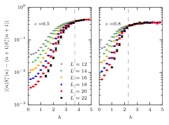
Figure 2: Disorder averaged difference of local magnetizations as a function of disorder strength in the middle (left) and upper part (right) of the spectrum. For weak disorder, eigenstates thermalize and the local magnetization of adjacent states becomes identical in the thermodynamic limit, thus yielding a smooth function of energy. Here, the mobility edge for the many body localization transition is also visible as the region, in which adjacent states yield very different results – the MBL phase – is much larger in the upper part of the spectrum at energy density $\epsilon=0.8$. The location of the previously estimatedLuitz et al. (2015) critical disorder strength $h_{c}\approx 3.7$ at $\epsilon=0.5$ and $h_{c}\approx 2.3$ at $\epsilon=0.8$ is given by the dashed line.

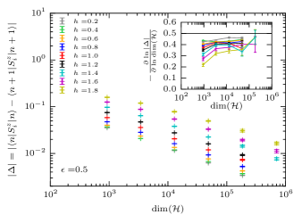
Figure 3: Finite size scaling of the disorder averaged difference of local magnetizations $\langle\,n\,|S_{z}^{i}|n\rangle$ of adjacent eigenstates as a function of the dimension of the Hilbert space $\text{dim}(\mathcal{H})$. The inset displays the (discrete) logarithmic derivative, yielding the exponent of the power law in the thermodynamic limit, which slowly approaches $0.5$. The data presented here includes only states from the middle of the spectrum ($\epsilon=0.5$).

III Local magnetization

Let us consider the simplest local operator to check the validity of the ETH: the local magnetization $\hat{S}_{i}^{z}$ on site $i$ of the system. The qualitative behavior of this quantity as a function of energy at intermediate disorder strength ($h=1.0$) is already clear from Fig. 1, where we show single eigenstate expectation values of $S_{5}^{z}$ at their corresponding energy density $\epsilon$ for different system sizes. Note that the disorder configuration of smaller system sizes is obtained as a subset of the larger sizes for comparability. In the middle of the spectrum, the data corresponds to $\gtrsim 50$ eigenstates obtained by a shift-invert technique, while for the largest system size $L=24$, we use a deflation technique for $\lesssim 2000$ states at the extreme ends of the spectrum, which successfully works down to $\epsilon=0.85$ for this size.

In Fig. 1 the variance of $\langle\,n\,|{\hat{S}_{i}^{z}}|n\rangle$ for eigenstates $|n\rangle$ at virtually the same energy decreases with system size for a wide range of the spectrum. It should be noted that the energy window in which the $\gtrsim 50$ eigenstates closest to the target energy lie decreases with system size, clearly visible by inspecting for example the $L=12$ and $L=16$ data. However, comparing data for adjacent targets suggests that the decreasing varianceIkeda et al. (2011); Khatami et al. (2012); Beugeling et al. (2014) of the local magnetization is not an artefact of the decreasing energy window size but rather a generic feature, leading to a well defined decrease of adjacent state local magnetization differences as shown in Fig. 2 with a power law in the dimension of the Hilbert space, that we analyze in Fig. 3 and discuss below.

At very high energy density, this is no longer true and the variance of this local observable over different eigenstates remains very large, thus breaking ETH. This is fully consistent with the many body mobility edge mapped in Ref. Luitz et al., 2015. Nevertheless, one should remain cautious with this observation as for the present disorder strength $h=1.0$ the mobility edge lies close to the boundary of the spectrum where finite size effects are expected to be large. Similarly, one expects a mobility edge at the low end of the spectrum, which is even more difficult to resolve due to stronger finite size effects, nevertheless the variance of $\langle\,n\,|\hat{S}_{5}^{z}|n\rangle$ does not seem to decrease between the two largest system sizes around $\epsilon\approx 0.1$.

In order to study the decreasing variance of the local magnetization more rigorously, we calculate the disorder average of the difference of $\hat{S}_{i}^{z}$ between an eigenstate $|n\rangle$ and the adjacent eigenstate $|n+1\rangle$. This quantity is a measure for the variance of the distribution of eigenstate expectation values of $\hat{S}_{i}^{z}$ over eigenstates within the microcanonical energy window around the target energy and over disorder realizations. It is obvious that the difference of local operators in adjacent eigenstates has to vanish if the quantity is to become a smooth function of energy in the thermodynamic limit. In Fig. 2, we show the disorder averaged difference of local magnetizations of adjacent eigenstates as a function of disorder strength for different system sizes. The signature of ETH is very clear as at weak disorder strength these differences scale to zero with increasing system size, whereas the breakdown of ETH in the MBL phase is signalled by a constant average difference for all system sizes. The position of the critical point that can be estimated from the point at which the ETH is no longer valid depends on the energy density and is fully consistent with a mobility edgeLuitz et al. (2015); Bera et al. (2015); Mondragon-Shem et al. (2015).

Previously, it has been established that the variance of eigenstate to eigenstate fluctuations of local operators in generic ETH systems decreases exponentially with system size as the square rootIkeda et al. (2011); Beugeling et al. (2014) of the dimension of the Hilbert space $\text{dim}(\mathcal{H})$. We verify this exponential law in Fig. 3 by plotting the average difference of adjacent eigenstate magnetizations $|\Delta_{m}|=|\langle\,n\,|S_{i}^{z}|n\rangle-\langle\,n+1\,|S_{i}^{z}|n+1\rangle|$ as a function of the dimension of the Hilbert space $\text{dim}(\mathcal{H})$ on a log-log scale. Our results are approximately linear and the corresponding exponent can be estimated by the (discrete) logarithmic derivative shown in the inset. We find exponents which are close to $-\frac{1}{2}$ for the largest system sizes, in agreement with the expectation of the square root behavior. The quality of the result is unfortunately not sufficient to back speculations if the deviations from an exponent of $-\frac{1}{2}$ are mere finite size effects or may have a deeper origin in the tails of the distributions to be discussed in Sec. V.

IV Generic few body operators

We have focussed on a specific local operator in the previous section: the local magnetization. This immediately leads to the question, whether different operators will also lead to a smooth function of energy and what condition these operators have to fulfill. In particular, we would like to investigate how “local” operators really have to be in order to fulfill ETH.

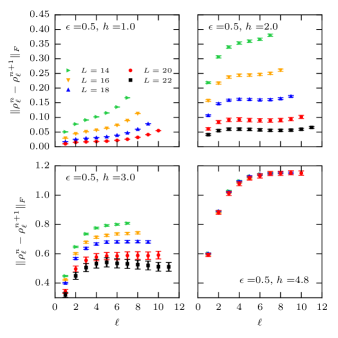
Figure 4: Disorder averaged Frobenius norm of the difference of reduced density matrices of a subsystem of size $\ell$ as a function of subsystem size.

All possible operators of a given support $\ell$ in two adjacent eigenstates $|n\rangle$ and $|n+1\rangle$ may be compared most efficiently by comparing the reduced density matricesAlba (2015); Garrison and Grover (2015)

$$\rho_{\ell}^{n}=\mathrm{Tr}_{\overline{A_{\ell}}}|n\rangle\langle\,n\,|,$$ (2)

where degrees of freedom corresponding to the complement of the subsystem $A_{\ell}$ are traced out. The expectation values in state $|n\rangle$ of all operators involving only degrees of freedom on $A_{\ell}$ are fully determined by $\rho_{\ell}^{n}$ and therefore if ETH requires them to become a smooth function of energy, the corresponding reduced density matrices of adjacent eigenstates have to become equal in the thermodynamic limit at least for “small” subsystem sizes. In Fig. 4, we show the Frobenius norm $\|\rho_{\ell}^{n}-\rho_{\ell}^{n+1}\|_{F}=\sqrt{\mathrm{Tr}\left[(\rho_{\ell}^{n}-\rho_{\ell}^{n+1})^{\dagger}(\rho_{\ell}^{n}-\rho_{\ell}^{n+1})\right]}$ of the difference of the reduced density matrices of adjacent eigenstates from the center of the spectrum ($\epsilon=0.5$), with the same subsystem of size $\ell$ as a function of $\ell$ (up to $\ell=L/2$) and observe that the reduced density matrices become indeed equal in the thermodynamic limit for astonishingly large subsystem sizes at weak disorder. This is quantitatively verified in Fig. 5, where we show the average reduced density matrix difference norm $\|\rho_{\ell}^{n}-\rho_{\ell}^{n+1}\|_{F}$ as a function of the dimension of the Hilbert space for different disorder strengths and $\ell=2$ (left) together with $\ell=6$ (right). As for the fluctuations of the local magnetization, the difference norm scales to zero as a power law with an exponent close to $-\frac{1}{2}$ (the inverse square root law is indicated by the slope of the black line). For intermediate disorder strengths the absolute value of the difference norm is larger but still decreases with system size, in agreement with the expectation that closer to the critical point systems with a fixed size $L$ suffer from larger finite size effects due to a larger correlation length.

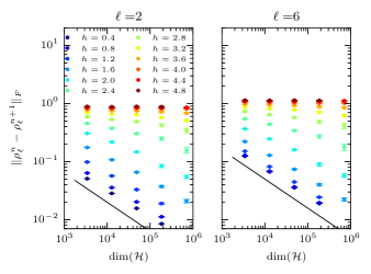
Figure 5: Disorder averaged norm of the difference of the reduced density matrices for adjacent eigenstates as a function of the dimension of the Hilbert space for two different subsystem sizes $\ell$ and different disorder strengths. The difference of the reduced density matrices decays as a power law in the dimension of the Hilbert space in the same way as the difference of local magnetizations in Fig. 3. The black line corresponds to $\leavevmode\nobreak\ \text{dim}(\mathcal{H})^{-\frac{1}{2}}$ for comparison and the exponent $-0.5$ is in good agreement with the results at weak disorder. In the MBL phase, the difference norm is constant with system size as expected.

We conclude that expectation values of operators with a support smaller than half of the system size may lead to smooth functions of energy in the ETH phase. Close to a subsystem size of $\ell=L/2$, we observe an increase of the difference norm with subsystem size, however we find the difference norm to be still smaller than the $L/2$ difference norm of the previous size.

V Probability distributions

Up to here, we have focussed on the behavior of disorder averages and concluded that in the ergodic phase of the random field Heisenberg chain ETH is valid on average. Let us now consider the approach to the thermodynamic limit in more detail and discuss the full probability distributions of the local magnetization difference $\Delta_{n,n+1}S_{i}^{z}$ of adjacent eigenstates as well as the entanglement entropy, showing that rare states exist which do not obey ETH in the sense that their fluctuations of local operators deviate from the normal distributionBeugeling et al. (2014) and that their weight will become more important with growing disorder strength. It is interesting to note that the presence of these non-ETH states coincides with the region of intermediate disorder of the phase diagram in which subdiffusive transport is observed. At the same time, we find that the probability distribution of the entanglement entropy exhibits low entanglement tails. The proposed mechanism for the explanation of subdiffusion relies on the argument that rare Griffiths region of localized spins exist, which act as bottlenecks for transportVosk et al. (2015); Potter et al. (2015). We expect that these localized regions lead to lower entanglement entropies if the entanglement cut lies within them and the observed low entanglement tails of the distribution are consistent with this scenario.

V.1 Probability distributions of eigenstate to eigenstate fluctuations

Let us first focus on the probability distribution of the differences of local magnetizations $\Delta_{n,n+1}S_{i}^{z}=|\langle\,n\,|S_{i}^{z}|n\rangle-\langle\,n+1\,|S_{i}^{z}|n+1\rangle|$ of adjacent eigenstates in the center of the spectrum ($\epsilon=0.5$) for different disorder strengths, shown in Fig. 6 for $L=20$. The argument in Ref. Beugeling et al., 2014 that eigenstate expectation values of local operators are effectively governed by the central limit theorem in generic ETH systems implies that one expects that the differences of the local magnetization in adjacent eigenstates are distributed according to a normal distribution with exponentially decreasing variance with system size and zero mean, while the microscopic origin of the randomness that justifies the applicability of the central limit theorem remains unclear. This is in fact verified to high accuracy at very weak disorder strength. For example in the top left panel of Fig. 7 for $h=0.4$ we show the histogram of $\Delta_{n,n+1}S_{i}^{z}$ for different system sizes and states in the center of the spectrum ($\epsilon=0.5$) together with best fits of the normal distribution, which seem to match perfectly with the numerical data.

However, starting at relatively small disorder strengths, deviations from the normal distribution emerge, as the distribution develops tails that are significantly heavier than those of the gaussian distribution.

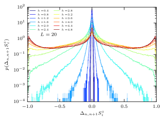
Figure 6: Probability density of the difference $\Delta_{n,n+1}S_{i}^{z}$ of the local magnetization $S_{z}^{i}$ of two eigenstates with adjacent energies for different disorder strenghts. The histograms are obtained from the central ($\epsilon=0.5$) 50 eigenstates of $10^{3}$ disorder realizations and contain the results for each site $i$ on which the local magnetization is compared. Even at very weak disorder, the distribution is already leptokurtic, showing heavier tails than the normal distribution. In the limit of very strong disorder, the distribution is dominated by the bimodal distribution of the local magnetization itself, which leads to the three dominant differences $-1,0,1$ stemming from random configurations of $S_{z}^{i}=-0.5,0.5$ in the MBL phase.

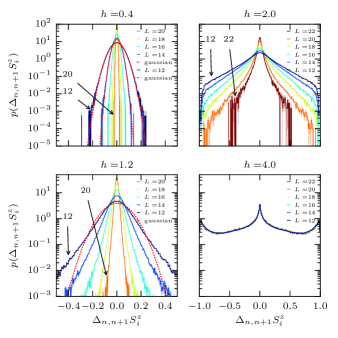
Figure 7: Probability density of the difference $\Delta_{n,n+1}S_{i}^{z}$ of the local magnetization $S_{z}^{i}$ of two eigenstates with adjacent energies for different system sizes and disorder strengths. For weak disorder, the reduction of the variance with system size is evident, however the distributions deviate increasingly from a gaussian distribution with growing disorder. In the MBL phase, the distributions become independent of system size, only governed by the localization length, which creates the nonzero weight between the three peaks of the distribution.

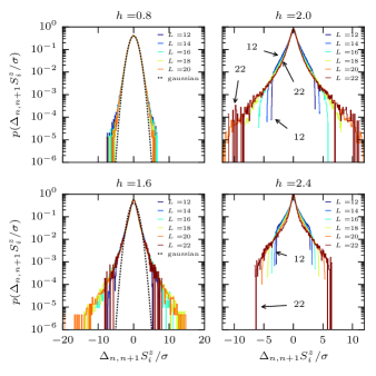
Figure 8: Probability density of the difference $\Delta_{n,n+1}S_{i}^{z}$ of the local magnetization $S_{i}^{z}$ of two eigenstates with adjacent energies, normalized by the standard deviation $\sigma$ to compare the shape of the distributions for different system sizes. For $h=0.8$, the weight of the tails seems to decrease with system size and approach the gaussian distribution. This is no longer true for stronger disorder and the weight of the tails increases strongly starting from $h\gtrsim 1.6$, accompanied by a growing kurtosis with system size in the same regime, making the distributions strongly leptokurtic. The kurtosis is defined by the fourth central moment divided by the squared variance, yielding a value of 3 for the gaussian distribution and larger values if the distribution has heavier tails, i.e. if it is leptokurtic.

While for weak disorder the deviations from the gaussian distribution seem to shrink with size, as seen e.g. in Fig. 8 for $h=0.8$, where we normalize the histograms by the standard deviation $\sigma$ to compare the shapes, this is no longer true at intermediate disorder, where the deviations from the gaussian distribution increase. In fact, for disorder strengths $h\gtrsim 1.6$, the weight of the tails actually grows with system size, pointing clearly to an effect that survives in the thermodynamic limit. This is most prominent in Fig. 8 for $h=2.0$ and $h=2.4$, where it seems that for the largest sizes we divide by a too large standard deviation, thus deforming the shape of the central peak, which narrows with system size, while the tails increase. This means that the variance is in fact larger than one would expect and is therefore influenced by the tails of the distribution, hinting for an effect that survives in the thermodynamic limit. On a more speculative note, this could be related to a slower scaling of the variances of the distribution to the thermodynamic limit as discussed in Figs. 3 and 5, modifying the exponent.

Interestingly, the distribution in the MBL phase at strong disorder becomes trimodal, indicating that local magnetizations of adjacent eigenstates are close to $\langle\,n\,|S_{i}^{z}|n\rangle=\pm\frac{1}{2}$ and completely independent, thus suggesting a binomial distribution at strong disorder , dressed by slight deviations caused by the finite support of the l-bits in terms of the localization length. As the localization length seems to be smaller than our system sizes already at $h=4.0$, we observe a distribution virtually independent of $L$ in Fig. 7.

V.2 Probability distributions of the entanglement entropy

One of the most studied quantities for the MBL transition is certainly the entanglement entropy, which is known to change its mean behavior from a thermal volume law in the ETH phase to an area law in the MBL phase. However, the probability distributions of the entanglement entropy have received less attention until recentlyVosk et al. (2015); Baygan et al. (2015); Lim and Sheng (2015), possibly due to the daunting requirement for the number of disorder realizations to obtain a satisfactory resolution of the histogram. Here, we show results for the probability distribution of the von Neumann entanglement entropy $S_{\text{E}}=-\mathrm{Tr}_{A}\left[(\mathrm{Tr}_{B}|n\rangle\langle\,n\,|)\ln(\mathrm{Tr}_{B}|n\rangle\langle\,n\,|)\right]$, where the subsystem $A$ represents half of the chain and $B$ is the complement of $A$. Averaging over approximately $>10^{3}$ disorder realizations, $\leavevmode\nobreak\ 50$ eigenstates per realization from the center of the spectrum ($\epsilon=0.5$) and over all cuts with subsystem size $L/2$, we can generate histograms from roughly $10^{6}$ samples of the entanglement entropy.

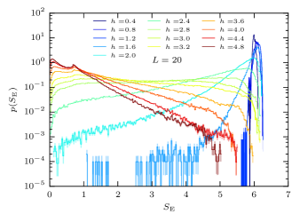
Figure 9: Probability density of the entanglement entropy $S_{E}$ of states in the middle of the spectrum ($\epsilon=0.5$) for different disorder strengths. We use the bipartition $L_{A}=L_{B}$ for the periodic $L=20$ chain. The evolution from the volume law behavior at weak disorder to the area law at strong disorder is clearly visible. At very weak disorder, the distribution is close to gaussian and develops exponential tails at intermediate disorder. They correspond to rare regions with low entanglement, responsible for slow (subdiffusive) transport.

The resulting histograms for different disorder strengths are shown in Fig. 9. For very weak disorder, the distribution is close to a normal distribution and the mode (position of the maximum) of the distribution increases slightly with increasing disorder, possibly due to the proximity to the integrable point at $h=0$, where additional integrals of motion restrict the degrees of freedom of eigenstates in the Hilbert space.

At weak to intermediate disorder strengths, the mode of the distribution is virtually unchanged but a long tail develops, reaching to extremely low values of entanglement. This corresponds to positions of the subsystem cut, where the two subsystems are virtually decoupled, leading to a product state of two smaller system eigenstates and a weak link between them. The weight of these very low entanglement cuts increases dramatically when approaching the transition, leading to a broad distribution with maximal variance around $h=3$. This distribution corresponds to the observed maximal variance of the entanglement entropy in the proximity of the critical pointKjäll et al. (2014); Luitz et al. (2015); Chen et al. (2015).

In the MBL phase, the mode of the distribution shifts to a very low (constant) value, creating the area (constant) law of the mean and develops a resonance at $S_{\text{E}}\approx\ln 2$, before showing a long exponential decay with arbitrarily strong entanglement. The peak close to zero entanglement reflects the fact that states are effectively product states in the l-bit basis, which becomes identical with the real space basis if the localization length becomes small enough at large disorder.

These results suggest that the environment of the transition in both ETH and MBL phases is governed by rare event effects, although their importance in the MBL phase is not clear as they may not be dominating the overall physics. The regime close to the critical point, dominated by Griffiths effects, has also recently been studied using a matrix product state based method to access larger system sizes in Ref. Lim and Sheng, 2015 together with exact diagonalization and the exponential tail of the distribution was also observed as well as a broad histogram at $h=3$.

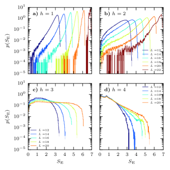
Figure 10: Probability density of the entanglement entropy $S_{E}$ of states in the middle of the spectrum for different system sizes at disorder strenghts a) $h=1$, b) $h=2$, c) $h=3$ and d) $h=4$.

Here, we try to connect the presence of low entanglement entropies, to the observed subdiffusive transport regimeLim and Sheng (2015); Vosk et al. (2015); Potter et al. (2015); Agarwal et al. (2015); Luitz et al. (2016) at intermediate disorder. The proposed mechanism for subdiffusion is via rare nearly localized regions, acting as bottlenecks for transport and the entanglement growth in time. If such regions exist, one would naturally expect that the entanglement entropy of the corresponding eigenstates will be low if the cut between the subsystems lies in such a rare region. In fact, one should note that one single localized region will only reduce the entanglement entropy by less than a factor of two, as it reduces entanglement only over one boundary of the subsystem down to the typical constant MBL entanglement entropy. As the total system has periodic boundaries, the second half of the entanglement entropy can still stem from the other subsystem boundary. Together with this argument, we conclude that we find the expected low entanglement entropies in the regime in which transport is subdiffusive and that our results are consistent with this scenario. In the next section, we will discuss this in further detail.

Let us briefly discuss the dependence on system size of the distributions of the entanglement entropy, shown in Fig. 10. At weak disorder strength ($h=1.0$), we observe a clear volume law and the importance of the low entanglement tail seems to decrease with growing system size, approaching more and more a normal distribution, although all the data for $L=22$ should be treated with care due to a number of samples that is by an order of magnitude smaller than for the other system sizes. At $h=2$ it is clear that the tail of the distribution extends all the way down to very low entanglement. On some very rare occasions, we observe nearly zero entanglement, which can only occur if the eigenstate is close to a product state or in other words if two localized regions fall exactly on the cut between the subsystems.

Interestingly, at $h=3$, before the estimated location of the critical point at $h\approx 3.7$, the distribution seems to become very broad, bounded by the maximal entanglement entropy, which is the reason for the observed maximum of the variance of entanglement entropy close to the critical pointKjäll et al. (2014); Luitz et al. (2015); Chen et al. (2015), here the weight of low entanglement states becomes very large and the behavior is dominated by rare region effects as discussed in Ref. Lim and Sheng, 2015. The dependence on system size suggests, however, that for even larger systems the mode of the distribution can still shift to the thermal value, leaving a large weight at low entanglement entropies.

In the MBL phase ($h=4$), the mode of the distribution is at a low (constant with system size) value, however the tail of the distribution grows with system size, reaching possibly up to the maximal entanglement entropy given by $L/2\ln 2$.

V.3 Weak links

Let us finally consider the spatial entanglement structure of the central eigenstates ($\epsilon=0.5$) in a typical disorder realization of length $L=22$ at intermediate disorder strength $h=2.0$.

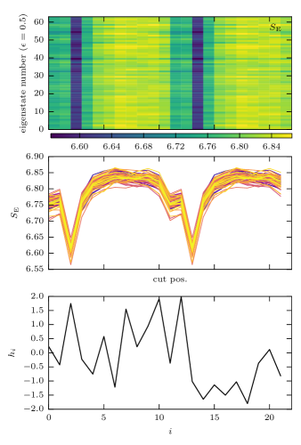
Figure 11: Top panel: Spatial variation of the entanglement entropy $S_{E}$ for the central 63 eigenstates of one disorder realization $h=2$ in the periodic $L=22$ chain (The disorder configuration ${h_{i}}$ as a function of the site index $i$ is shown in the bottom panel.) as a function of the position of the cut between subsystem $A$ and $B$. The subsystem size is $\ell=L/2$. Center panel: Same data as in the top panel as line graph. Depending on the cut position, the entanglement entropy varies and is found to be particularly low for some cuts, corresponding to a weaker link between the subsystems.

We show in the top panel of Fig. 11 for the central 63 eigenstates the entanglement entropy as a function of the cut position for all 22 possible cut positions (of which the second half is naturally equivalent to the first half). This representation reveals an intriguing feature: all states show a minimal entanglement entropy if the system is cut between spins 1 and 2 (the second cut is between spins 12 and 13), while the entanglement entropy is larger for other cut positions. Although in this sample the drop in the entanglement entropy is not very large, it is interesting to observe that the spatial structure is identical in all eigenstates in the energy window. This means that the entanglement across one of the boundaries of the subsystem is slightly smaller for all eigenstates and could be caused by a weak link, possibly leading to slightly slower transport. One would expect that such a weak link is caused by a field configuration that localizes spins through large fields and the corresponding configuration in the lower panel of Fig. 11 suggests that this may be caused by the large field $h_{i}$ on spin 12 and to a lesser extent on spin 2, in fact, a comparison of many samples leads to the hypothesis that a large change in the field configuration may lead to a weak link.

In Fig. 12, we present a sample at $h=3$, $L=18$, where the effect is much more severe: Here, the entanglement entropy is reduced roughly by a factor of 2 for most states if the cut lies between spins 2 and 3 and spins 11 and 12, compared to other cuts. Again, the spatial correlation between all states is visible and maximal field changes on both boundaries of the subsystem at spins 2 and 11 may be responsible for the weak link.

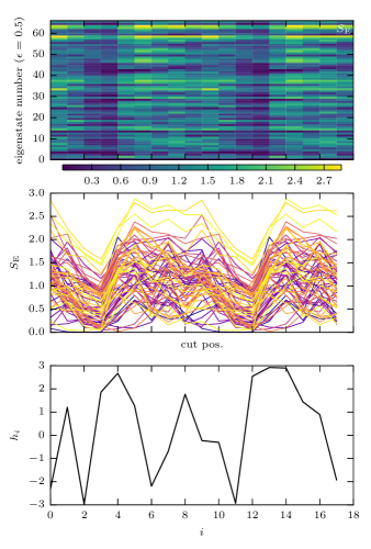
Figure 12: Top panel: Spatial variation of the entanglement entropy $S_{E}$ for the central 67 eigenstates of one disorder realization $h=3$ in the periodic $L=18$ chain (The disorder configuration ${h_{i}}$ as a function of the site index $i$ is shown in the bottom panel.) as a function of the position of the cut between subsystem $A$ and $B$. The subsystem size is $\ell=L/2$. Center panel: Same data as in the top panel as line graph. Depending on the cut position, the entanglement entropy varies and is found to be particularly low for some cuts, corresponding to a weaker link between the subsystems.

Let us also mention that the correlation of the entanglement profile in all eigenstates has also been observed in Ref. Bera and Lakshminarayan, 2015 by the nearest neighbor concurrence as a measure of entanglement. Our results show that the low entanglement tails in the distribution of the entanglement entropy in the ETH phase are not simply caused by low entanglement states (which do also exist) but are at least partly created by a spatial variation of the entanglement entropy as a function of the positions of the subsystem boundaries. The effect is the strongest if at least two localized regions are present at a distance that corresponds to the subsystem length.

VI Conclusion

We have studied in detail the validity of the eigenstate thermalization hypothesis in the random field Heisenberg chain and find that while typical states in the ergodic phase obey ETH, there are rare states with local expectation values far from the ETH mean, leading to tails of the fluctuation distributions that are significantly heavier than those of the normal distribution.

A comparison of distributions for different system sizes shows that the ETH violating tails can survive in the thermodynamic limit, as at intermediate disorder strength the weight of the tails can even increase with system size. This coincides with the region of the phase diagram that has been reported to be dominated by Griffiths effectsAgarwal et al. (2015); Vosk et al. (2015); Potter et al. (2015); Luitz et al. (2016); Laumann et al. (2014); Lim and Sheng (2015) close to the MBL transition.

Similar rare event tails are also observed in the distribution of the entanglement entropy, which become dominant close to the critical point, creating the large variance of the entanglement entropy that has been reported previouslyKjäll et al. (2014); Luitz et al. (2015); Chen et al. (2015). We argue that at least a part of the weight of the tails of the distribution is caused by the spatial entanglement structure, showing typical disorder realizations that have a large intrinsic variance of the entanglement entropy, when changing the position of the cut between the subsystems. This observation is in agreement with the proposed mechanism for subdiffusive transport, which relies on rare localized regions that act as weak links.

While it is consistent with other studies that low entanglement regions in the ergodic phase may be the cause of the anomalous transport properties at intermediate disorder, it remains an open question if the MBL phase has pathological properties close to the transition due to rare high entanglement regions. The presently accessible system sizes also leave the question of the shape of the distribution at the critical point unanswered. On a final note, we mention that close to the transition, the observed high entanglement tails in the MBL phase might be problematic for matrix product state based methodsYu et al. (2015); Khemani et al. (2015); Lim and Sheng (2015); Kennes and Karrasch (2015), requiring larger bond dimensions.