Weak decays of heavy hadrons into dynamically generated resonances

Abstract

We present a review of recent works on weak decay of heavy mesons and baryons with two mesons, or a meson and a baryon, interacting strongly in the final state. The aim is to learn about the interaction of hadrons and how some particular resonances are produced in the reactions. It is shown that these reactions have peculiar features and act as filters for some quantum numbers which allow to identify easily some resonances and learn about their nature. The combination of basic elements of the weak interaction with the framework of the chiral unitary approach allow for an interpretation of results of many reactions and add a novel information to different aspects of the hadron interaction and the properties of dynamically generated resonances.

1 Introduction

In this review we give a perspective of the theoretical work done recently on the interpretation of results from $B$, $D$, $\Lambda_{b}$, $\Lambda_{c}$ weak decays into final states that contain interacting hadrons, and how it is possible to obtain additional valuable information that is increasing our understanding of hadron interactions and the nature of many hadronic resonances. The novelty of these processes is that one begins with a clean picture at the quark level which allows one to select the basic mechanisms by means of which the process proceeds. Finally, one has a final state described in terms of quarks. To make contact with the experiments, where mesons and baryons are observed, one must hadronize, creating pairs of $q\bar{q}$ and writing the new states in terms of mesons and baryons. This concludes the primary hadron production in these processes. After that, the interaction of these hadrons takes place, offering a rich spectrum of resonances and special features from where it is possible to learn much about the interaction of these hadrons and the nature of many resonances in terms of the components of their wave functions.

2 The scalar sector in the meson-meson interaction

Let us begin with some examples where the low-lying scalar meson resonances are produced. This will include $B^{0}$ and $B^{0}_{s}$ decays into $J/\psi$ $f_{0}(500)$ and $J/\psi$ $f_{0}(980)$ and $D^{0}$ decay into $K^{0}$ and $f_{0}(500)$, $f_{0}(980)$ and $a_{0}(980)$.

The $f_{0}(500)$, $f_{0}(980)$ and $a_{0}(980)$ resonances have been the subject of discussion for years with an apparently endless debate whether they are $q\bar{q}$ states, tetraquarks, molecular systems, etc. [1, 2]. The advent of the chiral unitary approach in different versions has brought some light into this issue. Our present position is the following: QCD at low energies can be described in terms of chiral Lagrangians in which the original quark and gluon degrees of freedom have been substituted by the hadrons observed in experiments, mesons and baryons [3, 4, 5, 6]. These Lagrangians involve pseudoscalar mesons and low-lying baryons, while vector mesons were included in Refs. Bando:1984ej,Bando:1987br,Meissner:1987ge. The extension of these ideas to higher energies of the order of GeV, incorporating unitarity in coupled channels, has brought new insight into this issue and has allowed one to provide answers to some of the questions raised concerning the nature of many resonances. With the umbrella of the chiral unitary approach we include works that use the coupled channels Bethe-Salpeter equation, or the inverse amplitude method, and by now are widely used in the baryon sector, where it was initiated[10, 11, 12, 13, 14, 15, 16, 17, 18, 19, 20, 21, 22, 23], and the meson sector [24, 25, 26, 27, 28, 29, 30, 31]. A recent thorough review on chiral dynamics and the nature of the low lying scalar mesons, in particular the $f_{0}(500)$, can be seen in Ref. Pelaez:2015qba.

The Bethe Salpeter (BS) equation for meson meson interaction in coupled channels reads as:

$$t=[1-VG]^{-1}V,$$ (1)

where $V$ is the transition matrix potential, usually taken as the lowest order amplitude of chiral perturbation theory (the inverse amplitude method includes explicitly terms of next order, but in the scalar sector the largest ones are generated by rescattering in the BS equation). These matrix elements for $\pi^{+}\pi^{-}$, $\pi^{0}\pi^{0}$, $K^{+}K^{-}$, $K^{0}\bar{K}^{0}$ can be taken for instance from Ref. Oller:1997ti and can be complemented with the matrix elements of the $\eta\eta$ channels from Ref. Gamermann:2006nm. Then the $t$ matrix provides the transition $t$ matrix from one channel to another. The diagonal $G$-matrix is constructed out of the loop function of two meson propagators:

$$G_{ii}(s)=i\int\frac{d^{4}q}{(2\pi)^{4}}\frac{1}{(P-q)^{2}-m^{2}_{1}+i\varepsilon}\,\frac{1}{q^{2}-m^{2}_{2}+i\varepsilon},$$ (2)

where $m_{1,2}$ are the masses of the two meson in channel $i$, and where $P^{2}\equiv s$ is the center of mass energy squared. This loop function can be regularized using a cutoff method or dimensional regularization. The interesting thing about these equations in the pseudoscalar sectors, with a suitable cut off of the order of 1 GeV to regularize the loops, is that one obtains an excellent description of all the observables in pseudoscalar-pseudoscalar meson interaction up to about 1 GeV. In particular one can also look for poles in the scattering matrix which lead to the resonances in the system. In this sense one obtains the $f_{0}(500)$, the $f_{0}(980)$ in $\pi\pi$ , the $a_{0}(980)$ in $\pi\eta$ and the $\kappa(800)$ in $K\pi$ in the s-wave matrix elements. Note that one neither puts the resonances by hand in the amplitudes, nor uses a potential that contains a seed of a pole via a CDD[34] pole term in the potential (of the type of $a/(s-s_{0})$). In this sense, these resonances appear in the same natural way as the deuteron appears in the solution of the Schrödinger equation for $NN$ scattering and qualify as dynamically generated states, kind of molecular meson–meson states. It is also interesting to evaluate the residues at the poles for each channel, for this tells us the strength of each channel in the wave function of the resonance. In this sense the $f_{0}(500)$ couples essentially to $\pi\pi$. The $f_{0}(980)$ couples most strongly to $K\bar{K}$, although this is a closed channel, pointing to the $K\bar{K}$ nature of this resonance, and it couples weakly to $\pi\pi$, the only open decay channel. The $a_{0}(980)$ couples strongly to $K\bar{K}$ and $\pi\eta$ and the $\kappa(800)$ to $K\pi$.

It is worth mentioning that in works where one starts with a $q\bar{q}$ seed to represent the scalars and then unitarizes the models to account for the inevitable coupling of these quarks to the meson meson components, it turns out that the meson meson components “eat up” the seed and they remain as the only relevant components of the wave function[35, 36, 37, 38].

3 The scalar meson sector in $B$ and $D$ decays

Let us begin with an example of application of the former ideas to interpret recent results from LHCb and other facilities.

The LHCb Collaboration measured the $B^{0}_{s}$ decays into $J/\psi$ and $\pi^{+}\pi^{-}$ and observed a pronounced peak for the $f_{0}(980)$[39]. At the same time the signal for the $f_{0}(500)$ was found very small or non-existent. The Belle Collaboration corroborated these results in Ref. Li:2011pg, providing absolute rates for the $f_{0}(980)$ production with a branching ratio of the order of $10^{-4}$. The CDF Collaboration confirmed these latter results in Ref. Aaltonen:2011nk. Further confirmation was provided by the D0 Collaboration in Ref. Abazov:2011hv. Furthermore, the LHCb Collaboration has continued working in the topic and in Ref. LHCb:2012ae results are provided for the $\bar{B}^{0}_{s}$ decay into $J/\psi$ $f_{0}(980)$ followed by the $\pi^{+}\pi^{-}$ decays of the $f_{0}(980)$. Here, again the $f_{0}(980)$ production is seen clearly while no evident signal is seen for the $f_{0}(500)$. Interestingly, in the analogous decay of $\bar{B}^{0}$ into $J/\psi$ and $\pi^{+}\pi^{-}$ [44] a signal is seen for the $f_{0}(500)$ production and only a very small fraction is observed for the $f_{0}(980)$ production, with a relative rate of about (1-10)% with respect to that of the $f_{0}(500)$ (essentially an upper limit is given). Further research has followed by the same collaboration and in Ref. Aaij:2014emv the $\bar{B}^{0}_{s}$ into $J/\psi$ and $\pi^{+}\pi^{-}$ is investigated. A clear peak is observed once again for $f_{0}(980)$ production, while the $f_{0}(500)$ production is not observed. The $\bar{B}^{0}$ into $J/\psi$ and $\pi^{+}\pi^{-}$ is further investigated in Ref. Aaij:2014siy with a clear contribution from the $f_{0}(500)$ and no signal for the $f_{0}(980)$.

To interpret these results we take the dominant mechanism for the weak decay of the $B$’s into $J/\psi$ and a primary $q\bar{q}$ pair, which is $d\bar{d}$ for $B^{0}$ decay and $s\bar{s}$ for $B^{0}_{s}$ decay. After this, this $q\bar{q}$ pair is allowed to hadronize into a pair of pseudoscalar mesons and we look at the relative weights of the different pairs of mesons. Once the production of these meson pairs has been achieved, they are allowed to interact, for what chiral unitary theory in coupled channels is used, and automatically the $f_{0}(500)$, $f_{0}(980)$ resonances are produced. We are then able to evaluate ratios of these production rates in the different decays studied[47] and we find indeed a striking dominance of the $f_{0}(500)$ in the $B^{0}$ decay and of the $f_{0}(980)$ in the $B^{0}_{s}$ decay, in a very good quantitative agreement with experiment.

3.1 Formalism

Following Ref. Stone:2013eaa we take the dominant weak mechanism for $\bar{B}^{0}$ and $\bar{B}^{0}_{s}$ decays (it is the same for $B^{0}$ and $B^{0}_{s}$ decays) which we depict in Fig. 1.

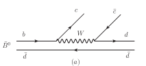
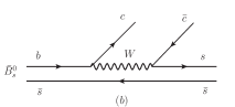
Figure 1: Diagrams for the decay of $\bar{B}^{0}$ and $\bar{B}^{0}_{s}$ into $J/\psi$ and a primary $q\bar{q}$ pair, $d\bar{d}$ for $\bar{B}^{0}$ and $s\bar{s}$ for $\bar{B}^{0}_{s}$.

In order to understand the process some very basic elements of the weak interaction are needed. The $W^{\pm}$ connects two quarks and the strength is given by the Cabibbo-Kobayashi-Maskawa (CKM) matrix[49, 50]. The operator resulting for the exchange of the $W$ in Fig. 1(a) is given by:[51, 52, 53]

$$H_{\rm W} = \frac{G_{F}}{\sqrt{2}}V_{bc}V_{cd}\bar{c}\gamma_{\mu}(1-\gamma_{5})b\bar{d}\gamma^{\mu}(1-\gamma_{5})c+h.c.$$ (3)

To get a feeling of the strength of the CKM matrix elements, recall that the quarks are classified in weak doublets

$$\left(\begin{array}[]{c}u\\ d\end{array}\right)\left(\begin{array}[]{c}c\\ s\end{array}\right)\left(\begin{array}[]{c}t\\ b\end{array}\right)$$

The transitions between quarks in the same doublet are Cabibbo allowed, they go roughly like the cosinus of the Cabibbo angle while from the first doublet to the second it goes like the sinus, concretely

$$V_{cd}=-\sin\theta_{c}=-0.22534,$$

$$V_{cs}=\cos\theta_{c}=0.97427.$$ (4)

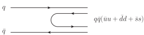
Figure 2: Schematic representation of the hadronization $q\bar{q}\to q\bar{q}(u\bar{u}+d\bar{d}+s\bar{s})$.

The differences between the two processes in Fig. 1 are: (i) $V_{cd}$ appears in the $Wcd$ vertex in $\bar{B}^{0}$ decay while $V_{cs}$ appears for the case of the $\bar{B}^{0}_{s}$ decay; (ii) one has a $d\bar{d}$ primary final hadron state in $\bar{B}^{0}$ decay and $s\bar{s}$ in $\bar{B}^{0}_{s}$ decay. Yet, one wishes to have $\pi^{+}\pi^{-}$ in the final state as in the experiments. For this we need the hadronization. This is easily accomplished: schematically this process is as shown in Fig. 2, where an extra $\bar{q}q$ pair with the quantum numbers of the vacuum, $\bar{u}u+\bar{d}d+\bar{s}s$, is added. Next step corresponds to writing the $q\bar{q}(\bar{u}u+\bar{d}d+\bar{s}s)$ combination in terms of pairs of mesons. For this purpose we define the $q\bar{q}$ matrix $M$,

$$M=\left(\begin{array}[]{ccc}u\bar{u}&u\bar{d}&u\bar{s}\\ d\bar{u}&d\bar{d}&d\bar{s}\\ s\bar{u}&s\bar{d}&s\bar{s}\\ \end{array}\right)$$ (5)

We can rewrite this in a different way and we see a nice property of this matrix

$$M =v\bar{v}=\left(\begin{array}[]{c}u\\ d\\ s\end{array}\right)\left(\begin{array}[]{ccc}\bar{u}&\bar{d}&\bar{s}\end{array}\right)=\left(\begin{array}[]{cccc}u\bar{u}&u\bar{d}&u\bar{s}\\ d\bar{u}&d\bar{d}&d\bar{s}\\ s\bar{u}&s\bar{d}&s\bar{s}\\ \end{array}\right)~{},$$ (13)

which fulfils:

$$M^{2} =(v\bar{v})(v\bar{v})=v(\bar{v}v)\bar{v}=\left(\bar{u}u+\bar{d}d+\bar{s}s\right)M~{}.$$ (14)

Now, in terms of mesons, the matrix $M$ corresponds to

$$\phi=\left(\begin{array}[]{ccc}\frac{1}{\sqrt{2}}\pi^{0}+\frac{1}{\sqrt{3}}\eta+\frac{1}{\sqrt{6}}\eta^{\prime}&\pi^{+}&K^{+}\\ \pi^{-}&-\frac{1}{\sqrt{2}}\pi^{0}+\frac{1}{\sqrt{3}}\eta+\frac{1}{\sqrt{6}}\eta^{\prime}&K^{0}\\ K^{-}&\bar{K}^{0}&-\frac{1}{\sqrt{3}}\eta+\sqrt{\frac{2}{3}}\eta^{\prime}\\ \end{array}\right)~{}.$$ (15)

This matrix corresponds to the ordinary one used in chiral perturbation theory [4] with the addition of $\frac{1}{\sqrt{3}}diag(\eta_{1},\eta_{1},\eta_{1})$ where $\eta_{1}$ is a singlet of $SU(3)$, taking into account the standard mixing between $\eta$ and $\eta^{\prime}$ [54, 55, 56]. The $\eta^{\prime}$ is omitted in the chiral Lagrangians because due to the $U_{A}(1)$ anomaly it is not a Goldstone Boson. Note also that the term $\frac{1}{\sqrt{3}}\text{diag}(\eta_{1},\eta_{1},\eta_{1})$ is inoperative in the $[\phi,\partial_{\mu}\phi]$ structure. In terms of two pseudoscalars we have the correspondence:

$$d\bar{d}(u\bar{u}+d\bar{d}+s\bar{s}) \equiv\left(\phi\cdot\phi\right)_{22}=\pi^{-}\pi^{+}+\frac{1}{2}\pi^{0}\pi^{0}-\frac{2}{\sqrt{6}}\pi^{0}\eta+K^{0}\bar{K}^{0}+\frac{1}{3}\eta\eta~{},$$

$$s\bar{s}(u\bar{u}+d\bar{d}+s\bar{s}) \equiv\left(\phi\cdot\phi\right)_{33}=K^{-}K^{+}+K^{0}\bar{K}^{0}+\frac{1}{3}\eta\eta~{},$$ (16)

where we have omitted the $\eta^{\prime}$ because of its large mass. We can see that $\pi^{+}\pi^{-}$ is only obtained in the first step in the $\bar{B}^{0}$ decay and not in $\bar{B}^{0}_{s}$ decay. However, upon rescattering of $K\bar{K}$ we also can get $\pi^{+}\pi^{-}$ in the final state, as we shall see. Yet, knowing that the $f_{0}(980)$ couples strongly to $K\bar{K}$ and the $f_{0}(500)$ to $\pi\pi$, the meson-meson decomposition of Eqs. (16) already tells us that the $\bar{B}^{0}$ decay will be dominated by $f_{0}(500)$ production and $\bar{B}^{0}_{s}$ decay by $f_{0}(980)$ production. Let us see how the interaction proceeds.

Let us call $V_{P}$ the production vertex which contains all dynamical factors common to both reactions. The $\pi^{+}\pi^{-}$ production will proceed via primary production or final state interaction as depicted in Fig. 3.

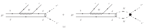
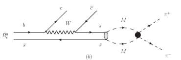
Figure 3: Diagrammatic representation of $\pi^{+}\pi^{-}$, via direct plus rescattering mechanisms in $\bar{B}^{0}$ decay (a), and via rescattering for $\bar{B}^{0}_{s}$ decay (b).

The amplitudes for $\pi^{+}\pi^{-}$ production are given by

$$t(\bar{B}^{0}\to J/\psi\pi^{+}\pi^{-}) =V_{P}V_{cd}(1+G_{\pi^{+}\pi^{-}}t_{\pi^{+}\pi^{-}\to\pi^{+}\pi^{-}}+2\frac{1}{2}\frac{1}{2}G_{\pi^{0}\pi^{0}}t_{\pi^{0}\pi^{0}\to\pi^{+}\pi^{-}}+$$

$$~{}~{}G_{K^{0}\bar{K}^{0}}t_{K^{0}\bar{K}^{0}\to\pi^{+}\pi^{-}}+2\frac{1}{3}\frac{1}{2}G_{\eta\eta}t_{\eta\eta\to\pi^{+}\pi^{-}}),$$

$$t(\bar{B}^{0}_{s}\to J/\psi\pi^{+}\pi^{-}) =V_{P}V_{cs}(G_{K^{+}K^{-}}t_{K^{+}K^{-}\to\pi^{+}\pi^{-}}+G_{K^{0}\bar{K}^{0}}t_{K^{0}\bar{K}^{0}\to\pi^{+}\pi^{-}}+$$

$$~{}~{}2\frac{1}{3}\frac{1}{2}G_{\eta\eta}t_{\eta\eta\to\pi^{+}\pi^{-}})~{},$$ (17)

where $G_{i}$ are the loop functions of two meson propagators defined above in Eq. (2). In Ref. Liang:2014tia a cut off $\Lambda=600$ MeV is taken, as needed in the enlarged space with respect to Ref. Oller:1997ti, including the $\eta\eta$ channel.

Note also that with respect to the weights of the meson-meson components in Eqs. (16) we have added a factor $1/2$ for the propagation of the $\pi^{0}\pi^{0}$ and $\eta\eta$ states which involve identical particles, and a factor of two for the two possible combinations to create two identical particles in the case of $\pi^{0}\pi^{0}$ or $\eta\eta$.

One comment is in order concerning Eq. (3.1), since in principle the $t$-matrices have left hand cut contributions while the form factors accounting for final state interaction which appear in the $B$ decay amplitudes do not have it. In Ref. [57] the problem of the form factors and its relationship to the chiral unitary aproach is addressed. A link is stablished there between the form factors and the $t$ matrices in the on shell factorization that we employ through our calculations, Eq. (1). The left hand cut contributions to the $t$ matrix are smoothly dependent on the energy for physical energies [58] and is usually taken into account by means of a constant added to the $G$ function. It is also interesting to recall the Quantum Mechanical version of this issue, which can be found in Ref. [59], and is basically equivalent to our approach using the on shell factorized $t$ matrices in Eq. (3.1).

One final element of information is needed to complete the formula for $d\Gamma/dM_{inv}$, with $M_{inv}$ the $\pi^{+}\pi^{-}$ invariant mass, which is the fact that in a $0^{-}\to 1^{-}0^{+}$ transition we shall need an $L^{\prime}=1$ for the $J/\psi$ to match angular momentum conservation. Hence, $V_{P}=A~{}p_{J/\psi}\cos\theta$, and we assume $A$ to be constant (equal to $1$ in the calculations). Thus,

$$\frac{d\Gamma}{dM_{inv}}=\frac{1}{(2\pi)^{3}}\frac{1}{4M_{\bar{B}_{j}}^{2}}\frac{1}{3}p_{J/\psi}^{2}p_{J/\psi}\tilde{p}_{\pi}{\overline{\sum}}\sum\left|\tilde{t}_{\bar{B}^{0}_{j}\to J/\psi\pi^{+}\pi^{-}}\right|^{2},$$ (18)

where the factor $1/3$ is coming from the integral of $\cos^{2}\theta$ and $\tilde{t}_{\bar{B}^{0}_{j}\to J/\psi\pi^{+}\pi^{-}}$ is $t_{\bar{B}^{0}_{j}\to J/\psi\pi^{+}\pi^{-}}/(p_{J/\psi}\cos\theta)$, which depends on the $\pi^{+}\pi^{-}$ invariant mass. In Eq. (18) $p_{J/\psi}$ is the $J/\psi$ momentum in the global CM frame ($\bar{B}$ at rest) and $\tilde{p}_{\pi}$ is the pion momentum in the $\pi^{+}\pi^{-}$ rest frame,

$$p_{J/\psi}=\frac{\lambda^{1/2}(M_{\bar{B}}^{2},M_{J/\psi}^{2},M_{inv}^{2})}{2M_{\bar{B}}},~{}~{}~{}~{}~{}~{}~{}\tilde{p}_{\pi}=\frac{\lambda^{1/2}(M_{inv}^{2},m_{\pi}^{2},m_{\pi}^{2})}{2M_{inv}},$$ (19)

with $\lambda(a,b,c)$ the Källen function.

3.2 Results

In Fig. 4 we show the $\pi^{+}\pi^{-}$ invariant mass distribution for the case of the $\bar{B}^{0}_{s}\to J/\psi\pi^{+}\pi^{-}$ decay, comparing the results with the data of Ref. Aaij:2014emv where more statistics has been accumulated than in the earlier run of Ref. Aaij:2011fx. The data are collected in bins of 20 MeV and the theoretical results are compared with the results in Fig. 14 of Ref. Aaij:2014emv. We can see that the agreement, up to an arbitrary normalization, is quantitatively good. We observe an appreciable peak for $f_{0}(980)$ production and basically no trace for $f_{0}(500)$ production. The agreement is even better with the dashed line in Fig. 14 of Ref. Aaij:2014emv where a small background has been subtracted. At invariant masses above the $f_{0}(980)$ peak, contribution from higher energy resonances, which we do not consider, is expected [45].

The second of Eqs. (3.1) tells us why the $f_{0}(500)$ contribution is so small. All intermediate states involved, $K\bar{K},\eta\eta$, have a mass in the $1~{}{\rm GeV}$ region and the $G$ functions are small at lower energies. Furthermore, the coupling of the $f_{0}(500)$ to both $K\bar{K}$ and $\eta\eta$ is also extremely small, such that the $t$ matrices involved have also small magnitudes.

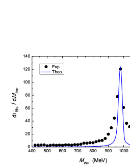
Figure 4: $\pi^{+}\pi^{-}$ invariant mass distribution for the $\bar{B}^{0}_{s}\to J/\psi\pi^{+}\pi^{-}$ decay, with arbitrary normalization and folded with a $20\ \text{MeV}$ resolution, compared with the data[45].

Note that in this decay we could have also $J/\psi$ and vector meson production, but the $s\bar{s}$ component would give $\phi$ production which does not decay to $\pi\pi$. The case is quite different for the $\bar{B}^{0}\to J/\psi\pi^{+}\pi^{-}$ decay, because now we can also produce $J/\psi\rho$ ($\rho\to\pi^{+}\pi^{-}$) decay and in fact this takes quite a large fraction of the $J/\psi\pi^{+}\pi^{-}$ decay, as seen in Ref. Aaij:2014siy. We shall address this point in the next section. We plot our relative $S$-wave $\pi^{+}\pi^{-}$ production for the $\bar{B}^{0}\to J/\psi\pi^{+}\pi^{-}$ decay in Fig. 5.

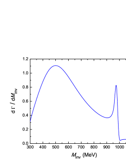
Figure 5: $\pi^{+}\pi^{-}$ invariant mass distribution for the $\bar{B}^{0}\to J/\psi\pi^{+}\pi^{-}$ decay, with arbitrary normalization. In a recent work,[60] there are small corrections of the order of 10$\%$ with respect to this figure, from considering the singlet contribution in Eq. (15), omitted in the work[47] reviewed here.

We can see that the $f_{0}(500)$ production is clearly dominant. The $f_{0}(980)$ shows up as a small peak. A test can be done to compare the results: If we integrate the strength of the two resonances over the invariant mass distribution we find

$$\frac{{\mathcal{B}}[\bar{B}^{0}\to J/\psi f_{0}(980),f_{0}(980)\to\pi^{+}\pi^{-}]}{{\mathcal{B}}[\bar{B}^{0}\to J/\psi f_{0}(500),f_{0}(500)\to\pi^{+}\pi^{-}]}=0.033\pm 0.007,$$ (20)

with an admitted 20% uncertainty from the decomposition of the strength in Fig. 5 into the two resonances. The most recent experimental result[46] is:

$$\left(0.6^{+0.7+3.3}_{-0.4-2.6}\right)\times 10^{-2}~{}.$$ (21)

The central value that we obtain is five times bigger than the central value of the experiment in Eq. (21), yet, by considering the errors in Eq. (21) we get a band for the experiment of $0\sim 0.046$ and our results are within this band. Let us note that in the work of [61], where a form factor is used, obtained using experimental phase shifts, one has a dip for the $f_{0}(980)$ following some enhancement in the strength of the distribution. We obtain a small, but neat peak for the $f_{0}(980)$, but also followed by a dip, which is not seen in the $B^{0}_{s}$ decay.

There is another point to consider. The normalization of Figs. 4 and  5 is arbitrary but the relative size is what the theory predicts. It is easy to compute

$$\frac{\Gamma(B^{0}\to J/\psi f_{0}(500))}{\Gamma(B^{0}_{s}\to J/\psi f_{0}(980))}\simeq\left(4.5\pm 1.0\right)\times 10^{-2}.$$ (22)

This number is in agreement within errors with the band of $(2.08\sim 4.13)\times 10^{-2}$ that one obtains from the branching fractions of $9.60^{+3.79}_{-1.20}\times 10^{-6}$ for $\bar{B}^{0}\to J/\psi f_{0}(500)$[44] and $3.40^{+0.63}_{-0.16}\times 10^{-4}$ for $\bar{B}^{0}_{s}\to J/\psi f_{0}(980)$[43].

Added to the results obtained for many other processes, as quoted in the Introduction, the present reactions come to give extra support to the idea originated from chiral unitary theory that the $f_{0}(500)$ and $f_{0}(980)$ resonances are dynamically generated from the interaction of pseudoscalar mesons and could be interpreted as a kind of molecular states of meson-meson with the largest component $\pi\pi$ for the $f_{0}(500)$ and $K\bar{K}$ for the $f_{0}(980)$.

Note that, while a better quantitative agreement in the shape of Fig 4 is obtained in [61] by using experimental $\pi\pi$ phase shifts in a big range of energies, the approach given here provides the basic features and allows to relate different decays processes without introducing further parameters.

So far we have assumed that $V_{P}$ is constant up to the $P$-wave factor. Actually there is a form factor for the transition that depends on the momentum transfer. Then it could be different for $f_{0}(500)$ or $f_{0}(980)$ production. However, the work in Refs. Li:2012sw,Ochs:2013gi,Kang:2013jaa indicates that the form factors for primary productions prior to the final state interaction, are rather smooth. This point gives us an excuse to elaborate on this issue and place our approach in a broader context. This is done in the next subsection.

3.3 Relationship to other approaches

Referring to the diagram in Fig. 1(b), the weak decay of a $b$ quark will proceed via the exchange of a $W^{\pm}$ which in one vertex will connect a $b$ and $c$ quark, and in the other vertex connect a $c$ and $s$ quark and the strength is given by the CKM matrix[50] elements. The operator resulting for the exchange of the $W$ is given[51, 52, 53] by:

$$H_{\rm W}=\frac{G_{F}}{\sqrt{2}}V_{cs}V_{bc}\bar{c}\gamma_{\mu}(1-\gamma_{5})b\bar{s}\gamma^{\mu}(1-\gamma_{5})c+h.c.$$ (23)

The theoretical study of these process requires the evaluation of the quark matrix elements of this operator for which many different approaches are followed. Quark models in different versions are one of the options[65, 66, 67, 68, 69]. Another approach using elements of QCD under the factorization approximation is followed in weak $B$ and $D$ decays into two final mesons [70, 71, 72, 73, 74, 75]. $B$ decays are also addressed in Ref. Colangelo:2010bg using light cone QCD sum rules under the factorization assumption. A different approach to $B^{0}$ into $J/\psi$ and $\pi^{+}\pi^{-}$ decay was followed in Ref. Sayahi:2013tza using the QCD-improved factorization approach.

Theoretical work on these issues is also done in Ref. Bediaga:2003zh for the semileptonic $D$ decays using QCD sum rules. The light-front quark model is used again in Ref. Ke:2009ed to calculate form factors for $D$ decays. A Nambu-Jona-Lasinio type model is used in Ref. Achasov:2012kk to study semileptonic $D$ decays. Estimations based on a simple model where the hadronic current is taken to be the Noether current associated with a minimal linear sigma model are also available for semileptonic $D$ decays[81, 82]. Research along similar lines is done in Ref. Wang:2009azc. Light-cone sum rules are used to evaluate the form factors appearing in different weak processes[84, 85, 86, 87, 88, 64, 89].

Apart from the hard processes that involve the weak transition and the hadronization, and that in QCD are considered in terms of the Wilson coefficients, one has to take into account the meson final state interaction. In some cases this is done using the Omnès representation[89, 85, 61], which have the advantage of preserving all good properties of unitarity and analyticity of the amplitudes. In other cases Breit–Wigner or Flatté structures are implemented and parametrized to account for the resonances observed in the experiment [84]. This latter procedure is known to have problems some times concerning these mentioned properties. Reference Doring:2013wka represents a hybrid approach insofar that unitarized chiral interactions are used to parameterize the $\pi K,\,\eta K$ amplitude, that is then fed into a dispersion approach to study semileptonic $B$ decays. For this, the two-channel inverse amplitude method of Ref. Oller:1998hw is considered that contains next-to-leading order contact terms, and that is supplemented with a resonance term to account for the $K_{0}^{*}(1430)$. The amplitude is fitted to $\pi K$ phase shift data. To guarantee the correct analytic structure, this amplitude serves then as input for a twice-subtracted Muskhelishvili-Omnès relation in the coupled $\pi K$ and $\eta K$ channels. Additionally, the form factor is matched to the value and slope of the one-loop ChPT result of the strangeness-changing form factors at $s=0$ [90].

In contrast to these pictures, in the present study we treat the meson–meson interaction using the chiral unitary approach.

In Fig. 1(b), after hadronization, Fig. 3(b), we have two mesons in the final state, in $S=0$, and we want to study their interaction. For this purpose, we encompass all the information of the hard transition part into a constant factor and, up to an arbitrary normalization, we obtain invariant mass distributions which are linked to the meson–meson interaction. The use of a constant $V_{P}$ factor in our approach gets support from the work of Ref. Daub:2015xja. The evaluation of the matrix elements in these processes is difficult and problematic, and we have given a sketch of the many different theoretical approaches for it. There are however some cases where the calculations can be kept under control. For the case of semileptonic decays with two pseudoscalar mesons in the final state with small recoil, namely when the final pseudoscalars move slowly, it can be explored in the heavy meson chiral perturbation theory[91]. Detailed calculations for the case of semileptonic decay are done in Ref. Kang:2013jaa. There one can see that for large values of the invariant mass of the lepton system the form factors can be calculated and the relevant ones in s wave that we need here are smooth in the range of the invariant masses of the pairs of mesons. In the present case the lepton system would be replaced by the $J/\psi$ which is very massive and extrapolating the results of Ref. Kang:2013jaa to this case one can conclude that the dependence of the s-wave matrix elements on the meson baryon invariant mass should be smooth. There is also another limit, at large recoil, where an approach that combines both hard-scattering and low-energy interactions has been developed and is also available[85], but this is not the case here.

There is also empirical information on the smoothness of these primary form factors. Yet, in Ref. Li:2012sw this form factor is evaluated for $B$ decays and it is found that $F^{\sigma}_{B^{0}_{s}}(m^{2}_{J/\psi})/F^{f_{0}}_{B^{0}_{s}}(m^{2}_{J/\psi})=1$, where $\sigma,f_{0}$ stand for the $f_{0}(500),f_{0}(980)$. In Ref. Ochs:2013gi the same results are assumed, as well as in Ref. Stone:2013eaa, where by analogy $F^{\sigma}_{B^{0}}(m^{2}_{J/\psi})/F^{f_{0}}_{B^{0}}(m^{2}_{J/\psi})$ is also assumed to be unity. In addition, in Ref. Stone:2013eaa it is also found from analysis of the experiment that $F^{f_{0}}_{B^{0}_{s}}(m^{2}_{J/\psi})/F^{\sigma}_{B^{0}}(m^{2}_{J/\psi})$ is compatible with unity.

All that one needs to apply our formalism is that the form factors for the primary production of hadrons prior to their final state interaction are smooth compared to the changes induced by this final state interaction. This is certainly always true in the vicinity of a resonance coming from this final state interaction, but the studies quoted above tell us that one can use a relatively broad range, of a few hundred MeV, where we still can consider these primary form factors smooth compared to the changes induced by the final state interaction.

4 Vector meson production

4.1 Formalism for vector meson production

At the quark level, we have

$$|\rho^{0}>=\frac{1}{\sqrt{2}}(u\bar{u}-d\bar{d});~{}~{}|\omega>=\frac{1}{\sqrt{2}}(u\bar{u}+d\bar{d});~{}~{}|K^{*0}>=d\bar{s}.$$ (24)

The diagrams of Fig. 1 without the hadronization can serve to study the production of vector mesons, which are largely $q\bar{q}$ states[92, 93, 94]. Since we were concerned up to now only about the ratio of the scalars, the factor $V_{P}$ was taken arbitrary. The spin of the particles requires now $L^{\prime}=0,2$, and with no rule preventing $L^{\prime}=0$, we assume that it is preferred; hence, the $p_{J/\psi}\cos\theta$ is not present now. Then we find immediately the amplitudes associated to Fig. 1,

$$t_{\bar{B}^{0}\rightarrow J/\psi\rho^{0}}=-\frac{1}{\sqrt{2}}\tilde{V}^{\prime}_{P}~{}V_{cd},~{} t_{\bar{B}^{0}\rightarrow J/\psi\omega}=\frac{1}{\sqrt{2}}\tilde{V}^{\prime}_{P}~{}V_{cd},~{} t_{\bar{B}^{0}_{s}\rightarrow J/\psi\phi}=\tilde{V}^{\prime}_{P}~{}V_{cs},$$

$$t_{\bar{B}^{0}\rightarrow J/\psi\bar{K}^{*0}}=\tilde{V}^{\prime}_{P}~{}V_{cs},~{} t_{\bar{B}^{0}_{s}\rightarrow J/\psi K^{*0}}=\tilde{V}^{\prime}_{P}~{}V_{cd},$$ (25)

where $(-\frac{1}{\sqrt{2}})$ is the $\rho^{0}$ component in $d\bar{d}$ and $(\frac{1}{\sqrt{2}})$ that of the $\omega$ and $\tilde{V}^{\prime}_{P}$ is the global factor for the processes, different to $V_{P}$ used for the scalar sector. In order to determine $\tilde{V}^{\prime}_{P}$ versus $V_{P}$ in the scalar production, we use the well-measured ratio[43, 95]:

$$\frac{\Gamma_{\bar{B}^{0}_{s}\rightarrow J/\psi f_{0}(980);f_{0}(980)\rightarrow\pi^{+}\pi^{-}}}{\Gamma_{\bar{B}^{0}_{s}\rightarrow J/\psi\phi}}=(13.9\pm 0.9)\times 10^{-2}.$$ (26)

The width for $J/\psi V$ vector decay is now given by

$$\Gamma_{V_{i}}=\frac{1}{8\pi}\frac{1}{m_{\bar{B}^{0}_{i}}^{2}}\left|t_{\bar{B}^{0}_{i}\to J/\psi V_{i}}\right|^{2}p_{J/\psi}.$$ (27)

Equations (25) allow us to determine ratios of vector production with respect to the $\phi$,

$$\frac{\Gamma_{\bar{B}^{0}\to J/\psi\rho^{0}}}{\Gamma_{\bar{B}^{0}_{s}\to J/\psi\phi}}=\frac{1}{2}\left|\dfrac{V_{cd}}{V_{cs}}\right|^{2}\dfrac{m_{\bar{B}^{0}_{s}}^{2}}{m_{\bar{B}^{0}}^{2}}\dfrac{p_{\rho^{0}}}{p_{\phi}}=0.0263,$$

$$\frac{\Gamma_{\bar{B}^{0}\to J/\psi\omega}}{\Gamma_{\bar{B}^{0}_{s}\to J/\psi\phi}}=\frac{1}{2}\left|\dfrac{V_{cd}}{V_{cs}}\right|^{2}\dfrac{m_{\bar{B}^{0}_{s}}^{2}}{m_{\bar{B}^{0}}^{2}}\dfrac{p_{\omega}}{p_{\phi}}=0.0263,$$ (28)

$$\frac{\Gamma_{\bar{B}^{0}\rightarrow J/\psi\bar{K}^{*0}}}{\Gamma_{\bar{B}^{0}_{s}\rightarrow J/\psi\phi}}=\dfrac{m_{\bar{B}^{0}_{s}}^{2}}{m_{\bar{B}^{0}}^{2}}\dfrac{p_{\bar{K}^{*0}}}{p_{\phi}}=0.957,$$

$$\frac{\Gamma_{\bar{B}_{s}^{0}\rightarrow J/\psi K^{*0}}}{\Gamma_{\bar{B}^{0}_{s}\rightarrow J/\psi\phi}}=\left|\dfrac{V_{cd}}{V_{cs}}\right|^{2}\dfrac{p_{K^{*0}}}{p_{\phi}}=0.0551.$$

By taking as input the branching ratio of $\bar{B}^{0}_{s}\rightarrow J/\psi\phi$,

$$BR(\bar{B}^{0}_{s}\rightarrow J/\psi\phi)=(10.0^{+3.2}_{-1.8})\times 10^{-4},$$ (29)

we obtain the other four branching ratios

$$BR(\bar{B}^{0}\rightarrow J/\psi\rho^{0})=(2.63^{+0.84}_{-0.47})\times 10^{-5},$$

$$BR(\bar{B}^{0}\rightarrow J/\psi\omega)=(2.63^{+0.84}_{-0.47})\times 10^{-5},$$

$$BR(\bar{B}^{0}\rightarrow J/\psi\bar{K}^{*0})=(9.57^{+3.1}_{-1.7})\times 10^{-4},$$

$$BR(\bar{B}_{s}^{0}\rightarrow J/\psi K^{*0})=(5.51^{+1.7}_{-1.0})\times 10^{-5}.$$ (30)

The experimental values are[95]:

$$BR(\bar{B}^{0}\rightarrow J/\psi\rho^{0})=(2.58\pm 0.21)\times 10^{-5},$$

$$BR(\bar{B}^{0}\rightarrow J/\psi\omega)=(2.3\pm 0.6)\times 10^{-5},$$

$$BR(\bar{B}^{0}\rightarrow J/\psi\bar{K}^{*0})=(1.34\pm 0.06)\times 10^{-3},$$

$$BR(\bar{B}_{s}^{0}\rightarrow J/\psi K^{*0})=(4.4\pm 0.9)\times 10^{-5}.$$ (31)

We can see that the agreement is good within errors, taking into account that the only theoretical errors in Eq. (30) are from the experimental branching ratio of Eq. (29). The rates discussed above have also been evaluated using perturbative QCD in the factorization approach in Ref. Liu:2013nea, with good agreement with experiment. Our approach exploits flavor symmetries and the dominance of the weak decay mechanisms of Fig. 1 to calculate ratios of rates with good accuracy in a very easy way.

The next step is to compare the $\rho$ production with $\rho\rightarrow\pi^{+}\pi^{-}$ decay with $\bar{B}^{0}\rightarrow J/\psi f_{0};f_{0}\rightarrow\pi^{+}\pi^{-}(f_{0}\equiv f_{0}(500),f_{0}(980)$). In an experiment that looks for $\bar{B}^{0}\rightarrow J/\psi\pi^{+}\pi^{-}$, all these contributions will appear together, and only a partial wave analysis will disentangle the different contributions. This is done in Refs. Aaij:2013zpt,Aaij:2014siy following the method of [97]. There (see Fig. 13 of Ref. Aaij:2014siy) one observes a peak of the $\rho$ and a $f_{0}(500)$ distribution, with a peak of the $\rho^{0}$ distribution about a factor $6$ larger than that of the $f_{0}(500)$. The $f_{0}(980)$ signal is very small and only statistically significant states are shown in the figure. Since only an upper limit was determined for the $f_{0}(980)$ it is not shown.

In order to compare the theoretical results with these experimental distributions, we convert the rates obtained in Eqs. (30) into $\pi^{+}\pi^{-}$ distributions for the case of the $\bar{B}^{0}\rightarrow J/\psi\rho^{0}$ decay and $K^{-}\pi^{+}$ for the case of the $\bar{B}^{0}\rightarrow J/\psi\bar{K}^{*0}$ decay. For this purpose, we multiply the decay width of the $\bar{B}^{0}$ by the spectral function of the vector mesons. We find:

$$\frac{d\Gamma_{\bar{B}^{0}\rightarrow J/\psi\rho^{0}}}{dM_{inv}(\pi^{+}\pi^{-})}=-\frac{1}{\pi}2M_{\rho}~{}{\rm Im}\dfrac{1}{M_{inv}^{2}-M_{\rho}^{2}+i~{}M_{\rho}\Gamma_{\rho}(M_{inv})}\Gamma_{\bar{B}^{0}\rightarrow J/\psi\rho^{0}},$$ (32)

where

$$\Gamma_{\rho}(M_{inv})=\Gamma_{\rho}\left(\dfrac{p_{\pi}^{\rm off}}{p_{\pi}^{\rm on}}\right)^{3},~{}~{}~{}p_{\pi}^{\rm off}=\dfrac{\lambda^{1/2}(M_{inv}^{2},m_{\pi}^{2},m_{\pi}^{2})}{2M_{inv}}\theta(M_{inv}-2m_{\pi}),$$

$$p_{\pi}^{\rm on}=\dfrac{\lambda^{1/2}(M_{\rho}^{2},m_{\pi}^{2},m_{\pi}^{2})}{2M_{\rho}}.$$ (33)

and for the case of the $\bar{B}^{0}\rightarrow J/\psi\bar{K}^{*0}~{}(\bar{K}^{*0}\rightarrow\pi^{+}K^{-})$, we have

$$\frac{d\Gamma_{\bar{B}^{0}\rightarrow J/\psi\bar{K}^{*0};\bar{K}^{*0}\rightarrow\pi^{+}K^{-}}}{dM_{inv}(\pi^{+}K^{-})} = -\frac{1}{\pi}\frac{2}{3}~{}{\rm Im}\dfrac{2M_{K^{*}}}{M_{inv}^{2}-M_{K^{*}}^{2}+i~{}M_{K^{*}}\Gamma_{K^{*}}(M_{inv})}$$ (34)

$$\times\Gamma_{\bar{B}^{0}\rightarrow J/\psi\bar{K}^{*0}},$$

with similar formulas for $\Gamma_{K^{*}}$, $p^{\rm off}$ and $p^{\rm on}$. In Eqs. (32) and (34) we have taken into account that $\rho^{0}$ decays only into $\pi^{+}\pi^{-}$, while $\bar{K}^{*0}$ decays into $\pi^{+}K^{-}$ and $\pi^{0}\bar{K}^{0}$ with weights $2/3$ and $1/3$, respectively. Expressions for $\bar{B}^{0}_{s}\to J/\psi K^{*0};K^{*0}\to\pi^{-}K^{+}$ are readily obtained from the previous ones with the obvious changes.

4.2 Results

In Fig. 6 we show our predictions for $f_{0}(500)$, $f_{0}(980)$, and $\rho^{0}$ production in $\bar{B}^{0}\to J/\psi\pi^{+}\pi^{-}$, taken from Ref. Bayar:2014qha.

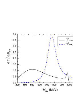
Figure 6: $\pi^{+}\pi^{-}$ invariant mass distributions for the $\bar{B}^{0}\to J/\psi\pi^{+}\pi^{-}$ ($S$ wave) (solid line) and $\bar{B}^{0}\to J/\psi\rho$, $\rho\to\pi^{+}\pi^{-}$ ($P$ wave) decays, with arbitrary normalization, and folded with a $20\ \text{MeV}$ resolution.

The relative strengths and the shapes of the $f_{0}(500)$ and $\rho$ distributions are remarkably similar to those found in the partial wave analysis of Ref. Aaij:2014siy. However, our $f_{0}(500)$ has a somewhat different shape since in the analysis of Ref. Aaij:2014siy, like in many experimental papers, a Breit-Wigner shape for the $f_{0}(500)$ is assumed, which is different to what the $\pi\pi$ scattering and the other production reactions demand[99, 100, 32]. It is interesting to remark that we have only considered the $\rho$ contribution without paying any attention to $\rho-\omega$ mixing. This is done explicitly in [61] and it leads to a peculiar shape, different to the one obtained in the electromagnetic form factor of the pion [57]. This new interesting shape is corroborated by a recent work [101]. It is also interesting to mention that, although small, we see a signal of the $f_{0}(980)$ in the distribution of Fig. 6, while in Daub:2015xja only a small bump is seen in this region. Let us mention to this respect that in the $J/\psi\to\omega\pi^{+}\pi^{-}$ decay, similar to the $B_{0}$ decay here, one observes clearly the $f_{0}(980)$ peak [102, 103] and there is a good agreement with the theoretical work of Roca:2004uc done along similar lines as here. It would be most interesting to see what one finds in the present case when more statistics is gathered.

In Fig. 7 we show the results for the Cabbibo allowed $\bar{B}^{0}\to J/\psi\pi^{+}K^{-}$, superposing the contribution of the $\bar{\kappa}$ and $\bar{K}^{*0}$ contributions and in Fig. 8 the results for the Cabbibo suppressed $\bar{B}_{s}^{0}\to J/\psi\pi^{-}K^{+}$, with the contributions of $\kappa$ and $K^{*0}$. The $\kappa(800)$ scalar contribution is calculated in Ref. Bayar:2014qha in the same way as described in the former subsection.

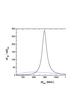
Figure 7: $\pi^{+}K^{-}$ invariant mass distributions for the $\bar{B}^{0}\to J/\psi\bar{K}^{*0}$, $\bar{K}^{*0}\to\pi^{+}K^{-}$ (solid line) and $\bar{B}^{0}\to J/\psi\bar{\kappa}$, $\bar{\kappa}\to\pi^{+}K^{-}$ (dashed line), with arbitrary normalization.

Figure 8: $\pi^{-}K^{+}$ invariant mass distributions for the $\bar{B}^{0}_{s}\to J/\psi K^{*0}$, $K^{*0}\to\pi^{-}K^{+}$ (solid line) and $\bar{B}^{0}_{s}\to J/\psi\kappa$, $\kappa\to\pi^{-}K^{+}$ (dashed line), with arbitrary normalization.

The narrowness of the $K^{*}$ relative to the $\rho$, makes the wide signal of the scalar $\kappa$ to show clearly in regions where the $K^{*0}$ strength is already suppressed. While no explicit mention of the $\kappa$ resonance is done in these $\bar{B}$ decays, in some analyses, a background is taken that resembles very much the $\kappa$ contribution that we have in Fig. 7 [105]. The $\kappa(800)$ appears naturally in chiral unitary theory of $\pi K$ and coupled channel scattering as a broad resonance around $800$ MeV, similar to the $f_{0}(500)$ but with strangeness [25]. In $D$ decays, concretely in the $D^{+}\rightarrow K^{-}\pi^{+}\pi^{+}$ decay, it is studied with attention and the links to chiral dynamics are stressed [106, 107]. With the tools of partial wave analysis developed in Ref. Aaij:2014siy, it would be interesting to give attention to this $S$-wave resonance in future analysis.

5 The low lying scalar resonances in the $D^{0}$ decays into $K^{0}_{s}$ and $f_{0}(500)$, $f_{0}(980)$, $a_{0}(980)$

5.1 Formalism

The process for $D^{0}\to K^{0}_{s}R$ proceeds at the elementary quark level as depicted in Fig. 9(A). The process is Cabibbo allowed, the $s\bar{d}$ pair produces the $\bar{K}^{0}$, which will convert to the observed $K^{0}_{s}$ through time evolution with the weak interaction. The remaining $u\bar{u}$ pair gets hadronized adding an extra $\bar{q}q$ with the quantum numbers of the vacuum, $\bar{u}u+\bar{d}d+\bar{s}s$. This topology is the same as for the $\bar{B}_{s}\to J/\psi s\bar{s}$ (substituting the $s\bar{d}$ by $c\bar{c}$) [48], that upon hadronization of the $s\bar{s}$ pair leads to the production of the $f_{0}(980)$ [47], which couples mostly to the hadronized $K\bar{K}$ components.

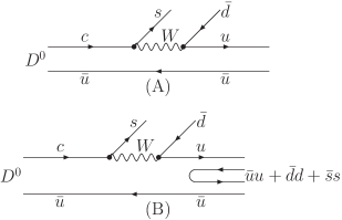
Figure 9: (A): Dominant diagram for $D^{0}\to\bar{K}^{0}u\bar{u}$ and (B): hadronization of the $u\bar{u}$ to give two mesons.

The hadronization is implemented as discussed previously. Hence upon hadronization of the $u\bar{u}$ component we shall have

$$u\bar{u}(\bar{u}u+\bar{d}d+\bar{s}s)\equiv(\phi\cdot\phi)_{11}=\frac{1}{2}\pi^{0}\pi^{0}+\frac{1}{3}\eta\eta+\frac{2}{\sqrt{6}}\pi^{0}\eta+\pi^{+}\pi^{-}+K^{+}K^{-}~{},$$ (35)

where we have omitted the $\eta^{\prime}$ term because of its large mass. This means that upon hadronization of the $u\bar{u}$ component we have $D^{0}\to\bar{K}^{0}PP$, where $PP$ are the different meson meson components of Eq. (35). This is only the first step, because now these mesons will interact among themselves delivering the desired meson pair component at the end: $\pi^{+}\pi^{-}$ for the case of the $f_{0}(500)$ and $f_{0}(980)$, and $\pi^{0}\eta$ for the case of the $a_{0}(980)$.

The multiple scattering of the mesons is readily taken into account as shown diagrammatically in Fig. 10.

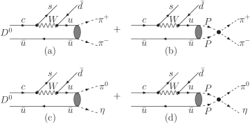
Figure 10: Diagrammatic representation of $\pi^{+}\pi^{-}$ and $\pi^{0}\eta$ production. (a) direct $\pi^{+}\pi^{-}$ production, (b) $\pi^{+}\pi^{-}$ production through primary production of a $PP$ pair and rescattering, (c) primary $\pi^{0}\eta$ production, (d) $\pi^{0}\eta$ produced through rescattering.

Analytically we shall have

$$t(D^{0}\to\bar{K}^{0}\pi^{+}\pi^{-}) = V_{P}(1+G_{\pi^{+}\pi^{-}}t_{\pi^{+}\pi^{-}\to\pi^{+}\pi^{-}}+2\frac{1}{2}\frac{1}{2}G_{\pi^{0}\pi^{0}}t_{\pi^{0}\pi^{0}\to\pi^{+}\pi^{-}}$$ (36)

$$+2\frac{1}{3}\frac{1}{2}G_{\eta\eta}t_{\eta\eta\to\pi^{+}\pi^{-}}+G_{K^{+}K^{-}}t_{K^{+}K^{-}\to\pi^{+}\pi^{-}}),$$

and

$$t(D^{0}\to\bar{K}^{0}\pi^{0}\eta)=V_{P}(\sqrt{\frac{2}{3}}+\sqrt{\frac{2}{3}}G_{\pi^{0}\eta}t_{\pi^{0}\eta\to\pi^{0}\eta}+G_{K^{+}K^{-}}t_{K^{+}K^{-}\to\pi^{0}\eta}),$$ (37)

where $V_{P}$ is a production vertex common to all the terms, and that encodes the underlying dynamics. $G$ is the loop function of two mesons [24] and $t_{ij}$ are the transition scattering matrices between pairs of pseudoscalars [24]. The $f_{0}(500)$, $f_{0}(980)$, and $a_{0}(980)$ are produced in $s$-wave where $\pi^{0}\pi^{0}$, $\pi^{+}\pi^{-}$ have isospin $I=0$, hence these terms do not contribute to $\pi^{0}\eta$ production ($I=1$) in Eq. (37). Note that in Eq. (36), as in former sections, we introduce the factor $\frac{1}{2}$ extra for the identity of the particles for $\pi^{0}\pi^{0}$ and $\eta\eta$, and a factor 2 for the two possible combinations to produce the two identical particles.

The $t$ matrix is obtained as discussed before and the matrix elements of the potential can be found in Ref. Xie:2014tma.

Finally, the mass distribution for the decay is given by Eq. (18) changing appropriately the variables. However, since we have a transition $0^{-}\to 0^{-}0^{+}$ we need $L=0$ now and the corresponding factor to $\frac{1}{3}p^{2}_{J/\psi}$ of Eq. (18) is omitted.

5.2 Results

In Fig. 11, we show the results for this process. We have taken the cut off $q_{\rm qmax}=600$ MeV as in Ref. Liang:2014tia. We superpose the two mass distributions $d\Gamma/dM_{\rm inv}$ for $\pi^{+}\pi^{-}$ (solid line) and $\pi^{0}\eta$ (dashed line). The scale is arbitrary, but it is the same for the two distributions, which allows us to compare $f_{0}(980)$ with $a_{0}(980)$ production. As we discussed before, it is a benefit of the weak interactions that we can see simultaneously both the $I=0$ $f_{0}(980)$ and $I=1$ $a_{0}(980)$ productions in the same $D^{0}\to\bar{K}^{0}R$ decay.

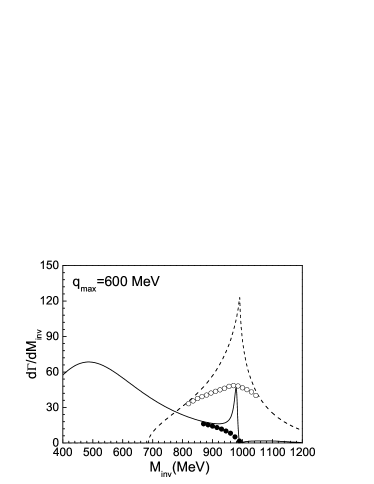
Figure 11: The $\pi^{+}\pi^{-}$ (solid line) and $\pi^{0}\eta$ (dashed line) invariant mass distributions for the $D^{0}\to\bar{K}^{0}\pi^{+}\pi^{-}$ decay and $D^{0}\to\bar{K}^{0}\pi^{0}\eta$ decay, respectively. A smooth background is plotted below the $a_{0}(980)$ and $f_{0}(980)$ peaks.

When it comes to compare with the experiment we can see that the $f_{0}(980)$ signal is quite narrow and it is easy to extract its contribution to the branching ratios by assuming a smooth background. For the case of the $\pi^{0}\eta$ distribution we get a clear peak that we associate to the $a_{0}(980)$ resonance, remarkably similar in shape to the one found in the experiment [109]. Not all the strength seen in Fig. 11 can be attributed to the $a_{0}(980)$ resonance. The chiral unitary approach provides full amplitudes and hence also background. In order to get a “$a_{0}(980)$” contribution we subtract a smooth background fitting a phase space contribution to the lower part of the spectrum. The remaining part has a shape with an apparent width of $80$ MeV, in the middle of the $50-100$ MeV of the PDG [95]. Integrating the area below these structures we obtain

$$R=\frac{\Gamma(D^{0}\to\bar{K}^{0}a_{0}(980),a_{0}(980)\to\pi^{0}\eta)}{\Gamma(D^{0}\to\bar{K}^{0}f_{0}(980),f_{0}(980)\to\pi^{+}\pi^{-})}= 6.7\pm 1.3,$$ (38)

where we have added a $20\%$ theoretical error due to uncertainties in the extraction of the background.

Experimentally we find from the PDG and the Refs. Muramatsu:2002jp,Rubin:2004cq,

$$\Gamma(D^{0}\to\bar{K}^{0}a_{0}(980),a_{0}(980)\to\pi^{0}\eta) = (6.5\pm 2.0)\times 10^{-3},$$ (39)

$$\Gamma(D^{0}\to\bar{K}^{0}f_{0}(980),f_{0}(980)\to\pi^{+}\pi^{-}) = (1.22^{+0.40}_{-0.24})\times 10^{-3}.$$ (40)

The ratio that one obtains from there is

$$R=5.33^{+2.4}_{-1.9}.$$ (41)

The agreement found between Eq. (38) and Eq. (41) is good, within errors. This is, hence, a prediction that we can do parameter free.

It should not go unnoticed that we also predict a sizeable fraction of the decay width into $D^{0}\to\bar{K}^{0}f_{0}(500)$, with a strength several times bigger than for the $f_{0}(980)$. The $\pi^{+}\pi^{-}$ distribution is qualitatively similar to that obtained in Ref. Liang:2014tia for the $\bar{B}^{0}\to J/\psi\pi^{+}\pi^{-}$ decay, although the strength of the $f_{0}(500)$ with respect to the $f_{0}(980)$ is relatively bigger in this latter decay than in the present case (almost $50\%$ bigger). A partial wave analysis is not available from the work of Ref. Muramatsu:2002jp, where the analysis was done assuming a resonant state and a stable meson, including many contributions, but not the $K^{0}_{s}f_{0}(500)$. Yet, a discussion is done at the end of the paper [110] in which the background seen is attributed to the $f_{0}(500)$. With this assumption they get a mass and width of the $f_{0}(500)$ compatible with other experiments. Further analyses in the line of Ref. Aaij:2014siy would be most welcome to separate this important contributions to the $D^{0}\to K^{0}_{s}\pi^{+}\pi^{-}$ decay.

5.3 Further considerations

Our results are based on the dominance of the quark diagrams of Fig. 9. In the weak decay of mesons the diagrams are classified in six different topologies [111, 112]: external emission, internal emission, $W$-exchange, $W$-annihilation, horizontal $W$-loop and vertical $W$-loop. As shown in Ref. Cheng:2010vk, only the internal emission graph (Fig. 9 of the present work) and $W$-exchange  contribute to the $D^{0}\to\bar{K}^{0}f_{0}(980)$ and $D^{0}\to\bar{K}^{0}a_{0}(980)$ decays. In Ref. Dedonder:2014xpa the $D^{0}\to\bar{K}^{0}\pi^{+}\pi^{-}$ decay is studied. Hence, only the $D^{0}\to K^{0}_{s}f_{0}(980)$ decay can be addressed, which is accounted for by proper form factors and taken into account by means of the $M_{2}$ ($K^{0}_{s}[\pi^{+}\pi^{-}]_{s}$) amplitude of that paper, which contains the tree level internal emission, and $W$-exchange (also called annihilation mechanism). We draw the external emission and $W$-exchange diagrams pertinent to the $D^{0}\to\bar{K}^{0}\pi^{+}\pi^{-}$ decay, as shown in Fig. 12.

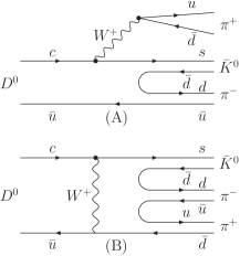
Figure 12: External emission diagram [(A)] and the $W$-exchange diagram [(B)] for $D^{0}\to\bar{K}^{0}\pi^{+}\pi^{-}$ decay

A discussion of the relevance of these diagrams is done in Ref. Xie:2014tma in connection to the work of Ref. Dedonder:2014xpa. The conclusion drawn there is that because the absorption diagrams involve two quarks of the original wave function, unlike the other mechanisms that have one of the quarks as spectators, these diagrams are small.

6 $\bar{B}^{0}$ decay into $D^{0}$ and $f_{0}(500)$, $f_{0}(980)$, $a_{0}(980)$, $\rho$ and $\bar{B}^{0}_{s}$ decay into $D^{0}$ and $\kappa(800)$, $K^{*0}$

In this section we report on the decay of $\bar{B}^{0}$ into $D^{0}$ and $f_{0}(500)$, $f_{0}(980)$, and $a_{0}(980)$. At the same time we study the decay of $\bar{B}^{0}_{s}$ into $D^{0}$ and $\kappa(800)$. We also relate the rates of production of vector mesons and compare $\rho$ with $f_{0}(500)$ production and $K^{*0}$ with $\kappa(800)$ production. Experimentally there is information on $\rho$ and $f_{0}(500)$ production in Ref. Kuzmin:2006mw for the $\bar{B}^{0}$ decay into $D^{0}$ and $\pi^{+}\pi^{-}$. There is also information on the ratio of the rates for $B^{0}\to\bar{D}^{0}K^{+}K^{-}$ and $B^{0}\to\bar{D}^{0}\pi^{+}\pi^{-}$ [116]. We investigate all these rates and compare them with the experimental information, following the work of Ref. Liang:2014ama.

6.1 Formalism

We show in Fig. 13 the dominant diagrams for $\bar{B}^{0}$ [Fig. 13 (a)] and $\bar{B}^{0}_{s}$ [Fig. 13 (b)] decays at the quark level. The mechanism has the $b\to c$ transition, needed for the decay, and the $u\to d$ vertex that requires the Cabibbo favored $V_{ud}$ CKM matrix element ($V_{ud}=\cos\theta_{c}$). Note that these two processes have the same two weak vertices. Under the assumption that the $\bar{d}$ in Fig. 13 (a) and the $\bar{s}$ in Fig. 13 (b) act as spectators in these processes, these amplitudes are identical.

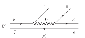
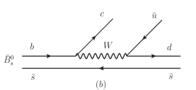
Figure 13: Diagrammatic representations of $\bar{B}^{0}\to D^{0}d\bar{d}$ decay (a) and $\bar{B}^{0}_{s}\to D^{0}d\bar{s}$ decay (b).

6.1.1 $\bar{B}^{0}$ and $\bar{B}^{0}_{s}$ decay into $D^{0}$ and a vector

Figure 13 (a) contains $d\bar{d}$ from where the $\rho$ and $\omega$ mesons can be formed. Figure 13 (b) contains $d\bar{s}$ from where the $K^{*0}$ emerges.

Hence, by taking as reference the amplitude for $\bar{B}^{0}\to D^{0}K^{*}$ as $V^{\prime}_{P}p_{D}$, we can write by using Eq. (24) the rest of the amplitudes as

$$t_{\bar{B}^{0}\to D^{0}\rho^{0}}=-\frac{1}{\sqrt{2}}V^{\prime}_{P}p_{D},$$ (42)

$$t_{\bar{B}^{0}\to D^{0}\omega}=\frac{1}{\sqrt{2}}V^{\prime}_{P}p_{D},$$ (43)

$$t_{\bar{B}^{0}\to D^{0}\phi}=0,$$ (44)

$$t_{\bar{B}^{0}_{s}\to D^{0}K^{*0}}=V^{\prime}_{P}p_{D},$$ (45)

where $V^{\prime}_{P}$ is a common factor to all $\bar{B}^{0}(\bar{B}^{0}_{s})\to D^{0}V_{i}$ decays, with $V_{i}$ being a vector meson, and $p_{D}$ the momentum of the $D^{0}$ meson in the rest frame of the $\bar{B}^{0}$ (or $\bar{B}^{0}_{s}$). The factor $p_{D}$ is included to account for a necessary $P$-wave vertex to allow the transition from $0^{-}\to 0^{-}1^{-}$. Although parity is not conserved, angular momentum is, and this requires the angular momentum $L=1$. Note that the angular momentum needed here is different than the one in the $\bar{B}^{0}\to J/\psi V_{i}$, where $L=0$. Hence, a mapping from the situation there to the present case is not possible.

The decay width is given by an expression equivalent to that of Eq. (27).

6.1.2 $\bar{B}^{0}$ and $\bar{B}^{0}_{s}$ decay into $D^{0}$ and a pair of pseudoscalar mesons

In order to produce a pair of mesons, the final quark-antiquark pair $d\bar{d}$ or $d\bar{s}$ in Fig. 13 has to hadronize into two mesons. The flavor content, which is all we need in our study, has been discussed in former sections: we must add a $\bar{q}q$ pair with the quantum numbers of the vacuum, $\bar{u}u+\bar{d}d+\bar{s}s$.

Following the developments in the former sections, we can write

$$d\bar{d}(\bar{u}u+\bar{d}d+\bar{s}s)\to(\phi\cdot\phi)_{22} = \pi^{-}\pi^{+}+\frac{1}{2}\pi^{0}\pi^{0}+\frac{1}{3}\eta\eta-\sqrt{\frac{2}{3}}\pi^{0}\eta+K^{0}\bar{K}^{0},$$ (46)

$$d\bar{s}(\bar{u}u+\bar{d}d+\bar{s}s)\to(\phi\cdot\phi)_{23} = \!\pi^{-}K^{+}-\!\frac{1}{\sqrt{2}}\pi^{0}K^{0},$$ (47)

where we have neglected the terms including $\eta^{\prime}$ that has too large mass to be relevant in our study.

Eqs. (46) and (47) give us the weight for pairs of two pseudoscalar mesons. The next step consists of letting these mesons interact, which they inevitably will do. This is done following the mechanism of Fig. 14.

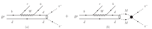
Figure 14: Diagrammatic representation of the final state interaction of the two mesons produced in a primary step. (a) Direct meson-meson production, (b) meson-meson production through rescattering.

The $f_{0}(500)$ and $f_{0}(980)$ will be observed in the $\bar{B}^{0}$ decay into $D^{0}$ and $\pi^{-}\pi^{+}$ final pairs, the $a_{0}(980)$ in $\pi^{0}\eta$ pairs and the $\kappa(800)$ in the $\bar{B}^{0}_{s}$ decay into $D^{0}$ and $\pi^{-}K^{+}$ pairs. Then we have for the corresponding production amplitudes

$$t(\bar{B}^{0}\to D^{0}\pi^{-}\pi^{+}) = V_{P}(1+G_{\pi^{-}\pi^{+}}t_{\pi^{-}\pi^{+}\to\pi^{-}\pi^{+}}+2~{}\frac{1}{2}\frac{1}{2}G_{\pi^{0}\pi^{0}}t_{\pi^{0}\pi^{0}\to\pi^{-}\pi^{+}}$$ (48)

$$+2~{}\frac{1}{3}\frac{1}{2}G_{\eta\eta}t_{\eta\eta\to\pi^{-}\pi^{+}}+G_{K^{0}\bar{K}^{0}}t_{K^{0}\bar{K}^{0}\to\pi^{-}\pi^{+}}),$$

where $V_{P}$ is a common factor of all these processes, $G_{i}$ is the loop function of two meson propagators, and we have included the factor $\frac{1}{2}$ and $2$ in the intermediate loops involving a pair of identical mesons, as done in the previous decays. The elements of the scattering matrix $t_{i\to j}$ are calculated in former sections following the chiral unitary approach of Refs. Oller:1997ti,Guo:2005wp. Note that the use of a common $V_{P}$ factor in Eq. (48) is related to the intrinsic $SU(3)$ symmetric structure of the hadronization $\bar{u}u+\bar{d}d+\bar{s}s$, which implicitly assumes that we add an $SU(3)$ $\bar{q}q$ singlet.

Similarly, we can also produce $K^{+}K^{-}$ pairs and we have

$$t(\bar{B}^{0}\to D^{0}K^{+}K^{-})=V_{P}(G_{\pi^{-}\pi^{+}}t_{\pi^{-}\pi^{+}\to K^{+}K^{-}}+2~{}\frac{1}{2}\frac{1}{2}G_{\pi^{0}\pi^{0}}t_{\pi^{0}\pi^{0}\to K^{+}K^{-}}$$

$$+2~{}\frac{1}{3}\frac{1}{2}G_{\eta\eta}t_{\eta\eta\to K^{+}K^{-}}-\sqrt{\frac{2}{3}}G_{\pi^{0}\eta}t_{\pi^{0}\eta\to K^{+}K^{-}}+G_{K^{0}\bar{K}^{0}}t_{K^{0}\bar{K}^{0}\to K^{+}K^{-}})~{}.$$ (49)

In the same way we can write

$$t(\bar{B}^{0}\to D^{0}\pi^{0}\eta)=V_{P}(-\sqrt{\frac{2}{3}}-\sqrt{\frac{2}{3}}G_{\pi^{0}\eta}t_{\pi^{0}\eta\to\pi^{0}\eta}+G_{K^{0}\bar{K}^{0}}t_{K^{0}\bar{K}^{0}\to\pi^{0}\eta}),$$ (50)

and taking into account that the amplitude for $\bar{B}^{0}_{s}\to c\bar{u}+d\bar{s}$ in Fig. 13 (b) is the same as for $\bar{B}^{0}\to c\bar{u}+d\bar{d}$ of Fig. 13 (a), and using Eq. (47) to account for hadronization, we obtain

$$t(\bar{B}^{0}_{s}\to D^{0}\pi^{-}K^{+})=V_{P}\big{(}1+ G_{\pi^{-}K^{+}}t_{\pi^{-}K^{+}\to\pi^{-}K^{+}}$$ (51)

$$-\frac{1}{\sqrt{2}} G_{\pi^{0}K^{0}}t_{\pi^{0}K^{0}\to\pi^{-}K^{+}}\big{)},$$

where the amplitudes $t_{\pi^{-}K^{+}\to\pi^{-}K^{+}}$ and $t_{\pi^{0}K^{0}\to\pi^{-}K^{+}}$ are taken from Ref. Guo:2005wp.

As in the former section, we have the transition $0^{-}\to 0^{-}0^{+}$ for $\bar{B}^{0}\to D^{0}f_{0}$, and now we need $L=0$. The differential invariant mass width is given again by Eq.(18) removing the factor $\frac{1}{3}p_{J/\psi}^{2}$ and adopting the appropriate masses.

6.2 Numerical results

In the first place we look for the rates of $\bar{B}^{0}$ and $\bar{B}^{0}_{s}$ decay into $D^{0}$ and a vector. By looking at Eqs. (42), (43), and (45), we have

$$\frac{\Gamma_{\bar{B}^{0}\to D^{0}\rho^{0}}}{\Gamma_{\bar{B}^{0}\to D^{0}\omega}}=\left[\frac{p_{D}(\rho^{0})}{p_{D}(\omega)}\right]^{3}=1,$$ (52)

$$\frac{\Gamma_{\bar{B}^{0}\to D^{0}\rho^{0}}}{\Gamma_{\bar{B}^{0}_{s}\to D^{0}K^{*0}}}=\left(\frac{M_{\bar{B}^{0}_{s}}}{M_{\bar{B}^{0}}}\right)^{2}\frac{1}{2}\left[\frac{p_{D}(\rho^{0})}{p_{D}(K^{*0})}\right]^{3}\simeq\frac{1}{2},$$ (53)

$$\Gamma_{\bar{B}^{0}\to D^{0}\phi}=0.$$ (54)

Experimentally there are no data in the PDG [95] for the branching ratio $Br({\bar{B}^{0}\to D^{0}\phi})$ and we find the branching ratios for $B^{0}\to\bar{D}^{0}\rho^{0}$ [115], $B^{0}\to\bar{D}^{0}\omega$ [119, 120], and $B^{0}_{s}\to\bar{D}^{0}\bar{K}^{*0}$ [121, 122, 115], as the following (note the change $\bar{B}^{0}\to B^{0}$ and $D^{0}\to\bar{D}^{0}$, $\bar{B}^{0}_{s}\to B^{0}_{s}$, $K^{*0}\to\bar{K}^{*0}$):

$$Br(B^{0}\to\bar{D}^{0}\rho^{0}) = (3.2\pm 0.5)\times 10^{-4},$$ (55)

$$Br(B^{0}\to\bar{D}^{0}\omega) = (2.53\pm 0.16)\times 10^{-4},$$ (56)

$$Br(B^{0}_{s}\to\bar{D}^{0}\bar{K}^{*0}) = (3.5\pm 0.6)\times 10^{-4}.$$ (57)

The ratio $\frac{\Gamma_{\bar{B}^{0}\to D^{0}\rho^{0}}}{\Gamma_{\bar{B}^{0}\to D^{0}\omega}}$ is fulfilled, while the ratio $\frac{\Gamma_{\bar{B}^{0}\to D^{0}\rho^{0}}}{\Gamma_{\bar{B}^{0}_{s}\to D^{0}K^{*0}}}$ is barely in agreement with data. The branching ratio of Eq. (57) requires combining ratios obtained in different experiments. A direct measure from a single experiment is available in Ref. Aaij:2011tz:

$$\frac{\Gamma_{\bar{B}^{0}_{s}\to D^{0}K^{*0}}}{\Gamma_{\bar{B}^{0}\to D^{0}\rho^{0}}}=1.48\pm 0.34\pm 0.15\pm 0.12,$$ (58)

which is compatible with the factor of $2$ that we get from Eq. (53). However, the result of Eq. (57), based on more recent measurements from Refs. Aaij:2014baa,Aaij:2013pua, improve on the result of Eq. (58)[124], which means that our prediction for this ratio is a bit bigger than experiment.

We turn now to the production of the scalar resonances. By using Eqs. (48)-(51), we obtain the mass distributions for $\pi^{+}\pi^{-}$, $K^{+}K^{-}$, and $\pi^{0}\eta$ in $\bar{B}^{0}$ decays and $\pi^{-}K$ in $\bar{B}^{0}_{s}$ decay. The numerical results are shown in Fig. 15.

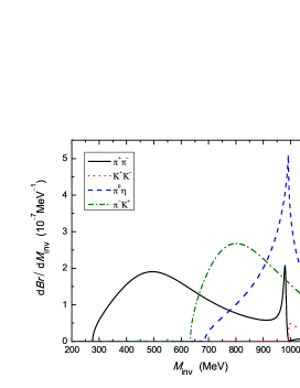
Figure 15: Invariant mass distributions for the $\pi^{+}\pi^{-}$, $K^{+}K^{-}$, and $\pi^{0}\eta$, and $\pi^{-}K$ in $\bar{B}^{0}\to D^{0}\pi^{+}\pi^{-}$, $D^{0}K^{+}K^{-}$, $D^{0}\pi^{0}\eta$, and $\bar{B}^{0}_{s}\to D^{0}\pi^{-}K^{+}$ decays. The normalization is such that the integral over the $f_{0}(500)$ signal gives the experimental branching ratio of Eq. (59).

The normalization for all the processes is the same. The scale is obtained demanding that the integrated $f_{0}(500)$ distribution has the normalization of the experimental branching ratio of Eq. (59). From Fig. 15, in the $\pi^{+}\pi^{-}$ invariant mass distribution for $\bar{B}^{0}\to D^{0}\pi^{+}\pi^{-}$ decay, we observe an appreciable strength for $f_{0}(500)$ excitation and a less strong, but clearly visible, for the $f_{0}(980)$. In the $\pi^{0}\eta$ invariant mass distribution, the $a_{0}(980)$ is also excited with a strength bigger than that of the $f_{0}(980)$. Finally, in the $\pi^{-}K^{+}$ invariant mass distribution, the $\kappa(800)$ is also excited with a strength comparable to that of the $f_{0}(500)$. We also plot the mass distribution for $K^{+}K^{-}$ production. It begins at threshold and gets strength from the two underlying $f_{0}(980)$ and $a_{0}(980)$ resonances, hence we can see an accumulated strength close to threshold that makes the distribution clearly different from phase space.

There is some experimental information to test some of the predictions of our results. Indeed in Ref. Kuzmin:2006mw (see Table II of that paper) one can find the rates of production for $f_{0}(500)$ [it is called $f_{0}(600)$ there] and $f_{0}(980)$. Concretely,

$$Br[\bar{B}^{0}\to D^{0}f_{0}(500)]\cdot Br[f_{0}(500)\to\pi^{+}\pi^{-}] = (0.68\pm 0.08)\times 10^{-4},$$ (59)

$$Br[\bar{B}^{0}\to D^{0}f_{0}(980)]\cdot Br[f_{0}(980)\to\pi^{+}\pi^{-}] = (0.08\pm 0.04)\times 10^{-4},$$ (60)

where the errors are only statistical. This gives

$$\left.\frac{Br[\bar{B}^{0}\to D^{0}f_{0}(980)]\cdot Br[f_{0}(980)\to\pi^{+}\pi^{-}]}{Br[\bar{B}^{0}\to D^{0}f_{0}(500)]\cdot Br[f_{0}(500)\to\pi^{+}\pi^{-}]}\right|_{\rm Exp.} = 0.12\pm 0.06.$$ (61)

From Fig. 15 it is easy to estimate our theoretical results for this ratio by integrating over the peaks of the $f_{0}(500)$ and $f_{0}(980)$. To separate the $f_{0}(500)$ and $f_{0}(980)$ contributions, a smooth extrapolation of the curve of Fig. 15 is made from 900 to 1000 MeV. We find

$$\left.\frac{Br[\bar{B}^{0}\to D^{0}f_{0}(980)]\cdot Br[f_{0}(980)\to\pi^{+}\pi^{-}]}{Br[\bar{B}^{0}\to D^{0}f_{0}(500)]\cdot Br[f_{0}(500)\to\pi^{+}\pi^{-}]}\right|_{\rm Theo.}=0.08,$$ (62)

with an estimated error of about 10%. As we can see, the agreement of the theoretical results with experiment is good within errors.

It is most instructive to show the $\pi^{+}\pi^{-}$ production combining the $S$-wave and $P$-wave production. In order to do that, we evaluate $V_{P}$ of Eq. (48) and $V^{\prime}_{P}$ of Eq. (42), normalized to obtain the branching fractions given in Eqs. (59) and (55), rather than widths. We shall call the parameters $\tilde{V}_{P}$ and $\tilde{V}^{\prime}_{P}$, suited to this normalization.

We obtain $\tilde{V}_{P}=(8.8\pm 0.5)\times 10^{-2}~{}{\rm MeV}^{-1/2}$ and $\tilde{V}^{\prime}_{P}=(6.8\pm 0.5)\times 10^{-3}~{}{\rm MeV}^{-1/2}$.

To obtain the $\pi^{+}\pi^{-}$ mass distribution for the $\rho$, we need to convert the total rate for vector production into a mass distribution. For that we follow the formalism developed in Section 4.

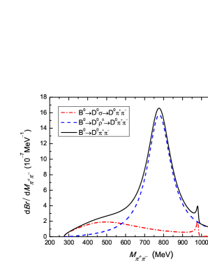
Figure 16: Invariant mass distribution for $\pi^{+}\pi^{-}$ in $\bar{B}^{0}\to D^{0}\pi^{+}\pi^{-}$ decay. The normalization is the same as in Fig. 15.

We show the results for the $\pi^{+}\pi^{-}$ production in $\bar{B}^{0}\to D^{0}\pi^{+}\pi^{-}$ in Fig. 16. We see a large contribution from the $f_{0}(500)$ and a larger contribution from the $\rho^{0}\to\pi^{+}\pi^{-}$ production. We can see that the $f_{0}(500)$ is clearly visible in the distribution of $\pi^{+}\pi^{-}$ invariant mass in the region of $400\sim 600$ MeV.

The $V_{P}$ and $V^{\prime}_{P}$ obtained by fitting the branching ratios of $f_{0}(500)$ and $\rho$ production can be used to obtain the strength of $K^{*0}$ production versus $\kappa(800)$ production in the $\bar{B}^{0}_{s}\to D^{0}\pi^{-}K^{+}$ decay. For this we use Eqs. (42)-(45) and recall that the rate for $K^{*0}\to\pi^{-}K^{+}$ is $\frac{2}{3}$ of the total $K^{*0}$ production. The results for $K^{*0}\to\pi^{-}K^{+}$ and $\kappa(800)\to\pi^{-}K^{+}$ production are shown in Fig. 17, where we see a clear peak for $K^{*0}$ production, with strength bigger than that for $\rho^{0}$ in Fig. 16, due in part to the factor-of-2 bigger strength in Eq. (53) and the smaller $K^{*0}$ width. The $\kappa(800)$ is clearly visible in the lower part of the spectrum where the $K^{*0}$ has no strength.

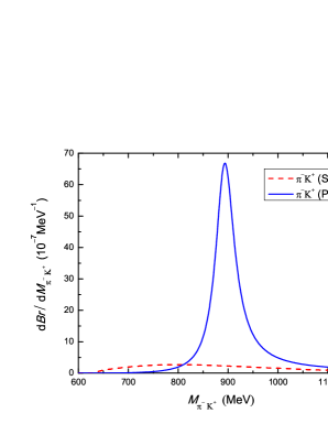
Figure 17: Invariant mass distribution for $\pi^{-}K^{+}$ in $\bar{B}^{0}_{s}\to D^{0}\pi^{-}K^{+}$ decay. The normalization is the same as in Fig. 15.

Finally, although with more uncertainty, we can also estimate the ratio

$$\frac{\Gamma(B^{0}\to\bar{D}^{0}K^{+}K^{-})}{\Gamma(B^{0}\to\bar{D}^{0}\pi^{+}\pi^{-})}=0.056\pm 0.011\pm 0.007$$ (63)

of Ref. Aaij:2012zka. This requires an extrapolation of our results to higher invariant masses where our results would not be accurate, but, assuming that most of the strength for both reactions comes from the region close to the $K^{+}K^{-}$ threshold and from the $\rho^{0}$ peak, respectively, we obtain a ratio of the order of $0.03\sim 0.06$, which agrees qualitatively with the ratio of Eq. (63).

7 $\bar{B}^{0}$ and $\bar{B}^{0}_{s}$ decays into $J/\psi$ and $f_{0}(1370)$, $f_{0}(1710)$, $f_{2}(1270)$, $f^{\prime}_{2}(1525)$, $K^{*}_{2}(1430)$

7.1 Vector- Vector interaction

In this section we describe the $\bar{B}^{0}$ and $\bar{B}^{0}_{s}$ decays into $J/\psi$ together with $f_{0}(1370)$, $f_{0}(1710)$, $f_{2}(1270)$, $f^{\prime}_{2}(1525)$, or $K^{*}_{2}(1430)$. The latter are resonances that are dynamically generated in the vector-vector interaction, which we briefly discuss now. In these interactions, an interesting surprise was found when using the local hidden gauge Lagrangians and, with a similar treatment to the one of the scalar mesons, new states were generated that could be associated with known resonances. This study was first conducted in the work of Ref. Molina:2008jw, where the $f_{0}(1370)$ and $f_{2}(1270)$ resonances were shown to be generated from the $\rho\rho$ interaction provided by the local hidden gauge Lagrangians [7, 8, 9] implementing unitarization. The work was extended to $SU(3)$ in Ref. Geng:2008gx and eleven resonances where dynamically generated, some of which were identified with the $f_{0}(1370)$, $f_{0}(1710)$, $f_{2}(1270)$, $f^{\prime}_{2}(1525)$ and $K^{*}_{2}(1430)$. The idea has been tested successfully in a large number of reactions and in Ref. Xie:2014gla a compilation and a discussion of these works have been done.

7.2 Formalism

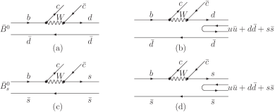
Figure 18: Basic diagrams for $\bar{B}^{0}$ and $\bar{B}^{0}_{s}$ decay into $J/\psi$ and a $q\bar{q}$ pair [(a) and (c)], and hadronization of the $q\bar{q}$ components [(b) and (d)].

As done in former sections we take the dominant mechanism for the decay of $\bar{B}_{0}$ and $\bar{B}^{0}_{s}$ into a $J/\psi$ and a $q\bar{q}$ pair. Posteriorly, this $q\bar{q}$ pair is hadronized into vector meson-vector meson components, as depicted in Fig. 18, and this hadronization is implemented as has already been explained in former sections.

In this sense the hadronized $d\bar{d}$ and $s\bar{s}$ states in Fig. 18 can be written as

$$d\bar{d}(\bar{u}u+\bar{d}d+\bar{s}s) = (M\cdot M)_{22},$$ (64)

$$s\bar{s}(\bar{u}u+\bar{d}d+\bar{s}s) = (M\cdot M)_{33}.$$ (65)

However, now it is convenient to establish the relationship of these hadronized components with the vector meson-vector meson components associated to them. For this purpose we write the matrix $M$ which has been defined in Eq. (13) in terms of the nonet of vector mesons:

$$V=\!\!\left(\!\!\begin{array}[]{ccc}\frac{\sqrt{2}}{2}\rho^{0}+\frac{\sqrt{2}}{2}\omega&\rho^{+}&K^{*+}\\ \rho^{-}&-\frac{\sqrt{2}}{2}\rho^{0}+\frac{\sqrt{2}}{2}\omega&K^{*0}\\ K^{*-}&\bar{K}^{*0}&\phi\\ \end{array}\!\!\right)~{},$$ (66)

and then we associate

$$d\bar{d}(\bar{u}u+\bar{d}d+\bar{s}s) \equiv (V\cdot V)_{22}=\rho^{-}\rho^{+}+\frac{1}{2}\rho^{0}\rho^{0}+\frac{1}{2}\omega\omega-\rho^{0}\omega+K^{*0}\bar{K}^{*0},$$ (67)

$$s\bar{s}(\bar{u}u+\bar{d}d+\bar{s}s) \equiv (V\cdot V)_{33}=K^{*-}K^{*+}+K^{*0}\bar{K}^{*0}+\phi\phi.$$ (68)

In the study of Ref. Geng:2008gx a coupled channels unitary approach was followed with the vector meson-vector meson states as channels. However, the approach went further since, following the dynamics of the local hidden gauge Lagrangians, a vector meson-vector meson state can decay into two pseudoscalars, $PP$. This is depicted in Figs. 19 (a), (b).

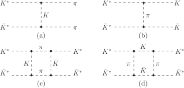
Figure 19: Decay mechanisms of $K^{*}\bar{K}^{*}+\pi\pi$, $K\bar{K}$ [(a) and (b)] and box diagrams considered[126] to account for these decays [(c) and (d)].

In Ref. Geng:2008gx these decay channels are taken into account by evaluating the box diagrams depicted in Figs. 19 (c), (d), which are assimilated as a part, $\delta\tilde{V}$, of the vector vector interaction potential $\tilde{V}$. This guarantees that the partial decay width into different channels could be taken into account.

Since we wish to have the resonance production and this is obtained through rescattering, the mechanism for $J/\psi$ plus resonance production is depicted in Fig. 20.

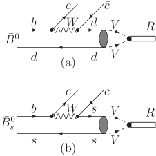
Figure 20: Mechanisms to generate the vector vector resonances through $VV$ rescattering. The dot of the vertex $RVV$ indicates the coupling of the resonance to the different $VV$ components.

The amplitudes for $J/\psi R$ production are then given by

$$t(\bar{B}^{0}\to J/\psi f_{0}) = \tilde{V}_{P}V_{cd}p_{J/\psi}{\rm cos}\theta(G_{\rho^{-}\rho^{+}}g_{\rho^{-}\rho^{+},f_{0}}+2\frac{1}{2}\frac{1}{2}G_{\rho^{0}\rho^{0}}g_{\rho^{0}\rho^{0},f_{0}}$$ (69)

$$+2\frac{1}{2}\frac{1}{2}G_{\omega\omega}g_{\omega\omega,f_{0}}+G_{K^{*0}\bar{K}^{*0}}g_{K^{*0}\bar{K}^{*0},f_{0}}),$$

$$t(\bar{B}^{0}_{s}\to J/\psi f_{0}) = \tilde{V}_{P}V_{cs}p_{J/\psi}{\rm cos}\theta(G_{K^{*0}\bar{K}^{*0}}g_{K^{*0}\bar{K}^{*0},f_{0}}$$ (70)

$$+G_{K^{*-}K^{*+}}g_{K^{*-}K^{*+},f_{0}}+2\frac{1}{2}G_{\phi\phi}g_{\phi\phi,f_{0}}),$$

where $G_{VV}$ are the loop functions of two vector mesons that we take from Ref. Geng:2008gx and $g_{VV,f_{0}}$ the couplings of $f_{0}$ to the pair of vectors $VV$, defined from the residues of the resonance at the poles

$$t_{ij}\simeq\frac{g_{i}g_{j}}{s-s_{R}},$$ (71)

with $t_{ij}$ the transition matrix from the channel $(VV)_{i}$ to $(VV)_{j}$. These couplings are also tabulated in Ref. Geng:2008gx. The formulas for the decay amplitudes to $J/\psi f_{2}$ are identical, substituting $f_{0}$ by $f_{2}$ in the formulas and the factor $\tilde{V}_{P}$ by a different one $\tilde{V}^{\prime}_{P}$ suited for the hadronization into a tensor. The magnitudes $\tilde{V}_{P}$ and $\tilde{V}^{\prime}_{P}$ represent the common factors to these different amplitudes which, before hadronization and rescattering of the mesons, are only differentiated by the CKM matrix elements $V_{cd}~{},V_{cs}$.

Note that as in former cases we include a factor $1/2$ in the $G$ functions for the $\rho^{0}\rho^{0}$, $\omega\omega$, and $\phi\phi$ cases and a factor 2 for the two combinations to create these states, to account for the identity of the particles. The factor $p_{J/\psi}{\rm cos}\theta$ is included there to account for a $p$-wave in the $J/\psi$ particle to match angular momentum in the $0^{-}\to 1^{-}0^{+}$ transition. The factor $p_{J/\psi}$ can however play some role due to the difference of mass between the different resonances.

The case for $\bar{B}^{0}\to J/\psi\bar{K}^{*}_{2}(1430)$ decay is similar. The diagrams corresponding to Figs. 18 (b), (d) are now written in Fig. 21.

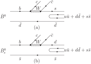
Figure 21: Mechanisms for $\bar{B}^{0}\to J/\psi\bar{K}^{*}_{2}(1430)$ and $\bar{B}^{0}_{s}\to J/\psi K^{*}_{2}(1430)$.

In analogy to Eqs. (67), (68) we now have

$$s\bar{d}(u\bar{u}+d\bar{d}+s\bar{s}) \equiv (V\cdot V)_{32}=K^{*-}\rho^{+}+\bar{K}^{*0}(-\frac{\rho^{0}}{\sqrt{2}}+\frac{\omega}{\sqrt{2}})+\bar{K}^{*0}\phi,$$ (72)

$$d\bar{s}(u\bar{u}+d\bar{d}+s\bar{s}) \equiv (V\cdot V)_{23}=\rho^{-}K^{*+}+(-\frac{\rho^{0}}{\sqrt{2}}+\frac{\omega}{\sqrt{2}})K^{*0}+K^{*0}\phi,$$ (73)

and the amplitudes for production of $J/\psi\bar{K}^{*}_{2}(1430)$ will be given by

$$t(\bar{B}^{0}\to J/\psi\bar{K}^{*}_{2}) = \tilde{V}^{\prime}_{P}p_{J/\psi}{\rm cos}\theta V_{cs}(G_{K^{*-}\rho^{+}}g_{K^{*-}\rho^{+},\bar{K}^{*}_{2}}-\frac{1}{\sqrt{2}}G_{\bar{K}^{*0}\rho^{0}}g_{\bar{K}^{*0}\rho^{0},\bar{K}^{*}_{2}}$$ (74)

$$+\frac{1}{\sqrt{2}}G_{\bar{K}^{*0}\omega}g_{\bar{K}^{*0}\omega,\bar{K}^{*}_{2}}+G_{\bar{K}^{*0}\phi}g_{\bar{K}^{*0}\phi,\bar{K}^{*}_{2}}),$$

$$t(\bar{B}^{0}_{s}\to J/\psi K^{*}_{2}) = \tilde{V}^{\prime}_{P}p_{J/\psi}{\rm cos}\theta V_{cd}(G_{K^{*+}\rho^{-}}g_{K^{*+}\rho^{-},K^{*}_{2}}-\frac{1}{\sqrt{2}}G_{\bar{K}^{*0}\rho^{0}}g_{\bar{K}^{*0}\rho^{0},K^{*}_{2}}$$ (75)

$$+\frac{1}{\sqrt{2}}G_{\bar{K}^{*0}\omega}g_{\bar{K}^{*0}\omega,K^{*}_{2}}\!\!+\!G_{\bar{K}^{*0}\phi}g_{\bar{K}^{*0}\phi,K^{*}_{2}}).$$

In Ref. Xie:2014gla these amplitudes are written in terms of the isospin amplitudes which are generated in Ref. Geng:2008gx. The width for these decays will be given by

$$\Gamma=\frac{1}{8\pi M^{2}_{\bar{B}}}|t|^{2}p_{J/\psi},~{}~{}~{}{\rm with}~{}~{}~{}p_{J/\psi}=\frac{\lambda^{1/2}(M^{2}_{\bar{B}},M^{2}_{J/\psi},M^{2}_{R})}{2M_{\bar{B}}}$$ (76)

with $M_{R}$ the resonance mass, and in $|t|^{2}$ we include the factor $1/3$ for the integral of ${\rm cos}\theta$, which cancels in all ratios that we will study.

The information on couplings and values of the $G$ functions, together with uncertainties is given in Table V of Ref. MartinezTorres:2009uk and Table I of Ref. Geng:2009iw. The errors for the scalar mesons production are taken from Ref. Geng:2009iw.

7.3 Results

In the PDG we find rates for $\bar{B}^{0}_{s}\to J/\psi f_{0}(1370)$ [43], $\bar{B}^{0}_{s}\to J/\psi f_{2}(1270)$ [43] and $\bar{B}^{0}_{s}\to J/\psi f^{\prime}_{2}(1525)$ [130]. We can calculate $10$ independent ratios and we have two unknown normalization constants $\tilde{V}_{P}$ and $\tilde{V}^{\prime}_{P}$. Then we can provide eight independent ratios parameter free. From the present experimental data we can only get one ratio for the $\bar{B}^{0}_{s}\to J/\psi f_{2}(1270)[f^{\prime}_{2}(1525)]$. There is only one piece of data for the scalars, but we should also note that the data for $\bar{B}^{0}_{s}\to J/\psi f_{0}(1370)$ in Ref. LHCb:2012ae and in the PDG, in a more recent paper [45] is claimed to correspond to the $f_{0}(1500)$ resonance. Similar ambiguities stem from the analysis of Ref. LHCb:2012ad.

The data for $f_{2}(1270)$ [43] and $f^{\prime}_{2}(1525)$ [130] of the PDG are

$$\Gamma(\bar{B}^{0}_{s}\to J/\psi f_{2}(1270)) = (10^{+5}_{-4})\times 10^{-7},$$ (77)

$$\Gamma(\bar{B}^{0}_{s}\to J/\psi f^{\prime}_{2}(1525)) = (2.6^{+0.9}_{-0.6})\times 10^{-4}.$$ (78)

However, the datum for $\Gamma(\bar{B}^{0}_{s}\to J/\psi f^{\prime}_{2}(1525))$ of the PDG is based on the contribution of only one helicity component $\lambda=0$, while $\lambda=\pm 1$ contribute in similar amounts.

This decay has been further reviewed in Ref. Aaij:2014emv and taking into account the contribution of the different helicities a new number is now provided, 

$$\Gamma(\bar{B}^{0}_{s}\to J/\psi f_{2}(1270))=\!\!(3.0^{+1.2}_{-1.0})\!\times\!\!10^{-6},$$ (79)

which is about three times larger than the one reported in the PDG (at the date of this review).

The results are presented in Table 1 for the eight ratios that we predict, defined as,

$$R_{1} = \frac{\Gamma[\bar{B}^{0}\to J/\psi f_{0}(1370)]}{\Gamma[\bar{B}^{0}\to J/\psi f_{0}(1710)]},~{}R_{2}=\frac{\Gamma[\bar{B}^{0}\to J/\psi f_{2}(1270)]}{\Gamma[\bar{B}^{0}\to J/\psi f^{\prime}_{2}(1525)]},$$

$$R_{3} = \frac{\Gamma[\bar{B}^{0}\to J/\psi f_{2}(1270)]}{\Gamma[\bar{B}^{0}\to J/\psi\bar{K}^{*}_{2}(1430)]},~{}R_{4}=\frac{\Gamma[\bar{B}^{0}\to J/\psi f_{0}(1710)]}{\Gamma[\bar{B}^{0}_{s}\to J/\psi f_{0}(1710)]},$$

$$R_{5} = \frac{\Gamma[\bar{B}^{0}\to J/\psi f_{2}(1270)]}{\Gamma[\bar{B}^{0}_{s}\to J/\psi f_{2}(1270)]},~{}R_{6}=\frac{\Gamma[\bar{B}^{0}_{s}\to J/\psi f_{0}(1370)]}{\Gamma[\bar{B}^{0}_{s}\to J/\psi f_{0}(1710)]},$$

$$R_{7} = \frac{\Gamma[\bar{B}^{0}_{s}\to J/\psi f_{2}(1270)]}{\Gamma[\bar{B}^{0}_{s}\to J/\psi f^{\prime}_{2}(1525)]},~{}R_{8}=\frac{\Gamma[\bar{B}^{0}_{s}\to J/\psi f_{2}(1270)]}{\Gamma[\bar{B}^{0}_{s}\to J/\psi K^{*}_{2}(1430)]}.$$

Table 1: Ratios of $\bar{B}^{0}$ and $\bar{B}^{0}_{s}$ decays.

Ratios	Theory	Experiment
$R_{1}$	$6.2\pm 1.6$	$--$
$R_{2}$	$13.4\pm 6.7$	$--$
$R_{3}$	$(3.0\pm 1.5)\times 10^{-2}$	$--$
$R_{4}$	$(7.7\pm 1.9)\times 10^{-3}$	$--$
$R_{5}$	$(6.4\pm 3.2)\times 10^{-1}$	$--$
$R_{6}$	$(1.1\pm 0.3)\times 10^{-2}$	$--$
$R_{7}$	$(8.4\pm 4.6)\times 10^{-2}$	$(1.0\sim 3.8)\times 10^{-2}$
$R_{8}$	$(8.2\pm 4.1)\times 10^{-1}$	$--$

Note that the different ratios predicted vary in a range of $10^{-3}$, such that even a qualitative level comparison with future experiments would be very valuable concerning the nature of the states as vector vector molecules, on which the numbers of the Tables are based.

The errors are evaluated in quadrature from the errors in Refs. MartinezTorres:2009uk,Geng:2009iw. In the case of $R_{7}$, where we can compare with the experiment, we put the band of experimental values for the ratio. The theoretical results and the experiment just overlap within errors.

From our perspective it is easy to understand the small ratio of these decay rates. The $f_{2}(1270)$ in Ref. Geng:2008gx is essentially a $\rho\rho$ molecule while the $f^{\prime}_{2}(1525)$ couples mostly to $K^{*}\bar{K}^{*}$. If one looks at Eq. (70) one can see that the $\bar{B}^{0}_{s}\to J/\psi f_{0}(f_{2})$ proceeds via the $K^{*}\bar{K}^{*}$ and $\phi\phi$ channels, hence, the $f_{2}(1270)$ with small couplings to $K^{*}\bar{K^{*}}$ and $\phi\phi$ is largely suppressed, while the $f^{\prime}_{2}(1525)$ is largely favored.

8 Learning about the nature of open and hidden charm mesons

The interaction of mesons with charm has also been addressed from the perspective of an extension of the chiral unitary approach. Meson meson interactions have been studied in many works[132, 133, 33, 134, 135, 136], and a common result is that there are many states that are generated dynamically from the interaction which can be associated to some known states, while there are also predictions for new states. Since then there have been ideas on how to prove that the nature of these states corresponds to a kind of molecular structure of some channels. The idea here is to take advantage of the information provided by the $B$ and $D$ decays to shed light on the nature of these states. We are going to show how the method works with two examples, one where the $D_{s0}^{\ast+}(2317)$ resonance is produced and the other one where some $X,Y,Z$ states are produced.

The very narrow charmed scalar meson $D_{s0}^{\ast+}(2317)$ was first observed in the $D_{s}^{+}\pi^{0}$ channel by the BABAR Collaboration [137, 138] and its existence was confirmed by CLEO [139], BELLE [140] and FOCUS [141] Collaborations. Its mass was commonly measured as $2317\text{ MeV}$, which is approximately $160\text{ MeV}$ below the prediction of the very successful quark model for the charmed mesons [142, 143]. Due to its low mass, the structure of the meson $D_{s0}^{\ast\pm}(2317)$ has been extensively debated. It has been interpreted as a $c\bar{s}$ state [144, 145, 146, 147, 148], two-meson molecular state [149, 150, 132, 133, 33, 134, 135, 136], $K-D$- mixing [151], four-quark states [152, 153, 154, 155] or a mixture between two-meson and four-quark states [156]. Additional support to the molecular interpretation came recently from lattice QCD simulations [157, 158, 159, 160]. In previous lattice studies of the $D_{s0}^{\ast}(2317)$, it was treated as a conventional quark-antiquark state and no states with the correct mass (below the $KD$ threshold) were found. In Refs. Mohler:2013rwa,Lang:2014yfa, with the introduction of $KD$ meson correlators and using the effective range formula, a bound state is obtained about 40 MeV below the $KD$ threshold. The fact that the bound state appears with the $KD$ interpolator may be interpreted as a possible $KD$ molecular structure, but more precise statements cannot be done. In Ref. Liu:2012zya lattice QCD results for the $KD$ scattering length are extrapolated to physical pion masses by means of unitarized chiral perturbation theory, and by means of the Weinberg compositeness condition [161, 162] the amount of $KD$ content in the $D_{s0}^{*}(2317)$ is determined, resulting in a sizable fraction of the order of 70% within errors. Yet, one should take this result with caution since it results from using one of the Weinberg compositeness[161] conditions in an extreme case. A reanalysis of the lattice spectra of Refs. Mohler:2013rwa,Lang:2014yfa has been recently done in Ref. Torres:2014vna, going beyond the effective range approximation and making use of the three levels of Refs. Mohler:2013rwa,Lang:2014yfa. As a consequence, one can be more quantitative about the nature of the $D_{s0}(2317)$, which appears with a $KD$ component of about 70%, within errors. Further works relating LQCD results and the $D^{\ast}_{s0}(2317)$ resonance can be found in Refs. Altenbuchinger:2013vwa,Altenbuchinger:2013gaa.

In addition to these lattice results, and more precise ones that should be available in the future, it is very important to have some experimental data that could be used to test the internal structure of this exotic state.

9 $D_{s0}^{\ast\pm}(2317)$ and $KD$ scattering from $B^{0}_{s}$ decay

Here we propose to use the experimental $KD$ invariant mass distribution of the weak decay of $\bar{B}_{s}^{0}\to D_{s}^{-}(DK)^{+}$ to obtain information about the internal structure of the $D_{s0}^{\ast+}(2317)$ state . There are not yet experimental data for the decay $\bar{B}^{0}_{s}\to D_{s}^{-}(DK)^{+}$. However, based on the 1.85% and 1.28% branching fractions for the decays $\bar{B}^{0}_{s}\to D_{s}^{*+}D_{s}^{*-}$ and $\bar{B}^{0}_{s}\to D_{s}^{+}D_{s}^{*-}+D_{s}^{*+}D_{s}^{-}$, the branching fraction for the $\bar{B}^{0}_{s}\to D_{s}^{-}D_{s0}^{\ast+}$ decay, should not be so different from that and be seen through the channel $\bar{B}^{0}_{s}\to D_{s}^{-}(DK)^{+}$. It is worth stressing that in the reactions $B^{0}\to D^{-}D^{0}K^{+}$ and $B^{+}\to\bar{D}^{0}D^{0}K^{+}$ studied by the BABAR Collaboration [165], an enhancement in the invariant $DK$ mass in the range $2.35-2.50\ \text{GeV}$ is observed, which could be associated with this $D_{s0}^{\ast+}(2317)$ state. It is also interesting to mention that, in the reaction $B^{0}_{s}\to\bar{D}^{0}K^{-}\pi^{+}$, the LHCb Collaboration also finds an enhancement close to the $KD$ threshold in the $\bar{D}^{0}K^{-}$ invariant mass distribution, which is partly associated to the $D_{s0}^{*}(2317)$ resonance [121].

Figure 22: Mechanism for the decay $\bar{B}^{0}_{s}\to D_{s}^{-}(DK)^{+}$.

In Fig. 22 we show the mechanism for the decay $\bar{B}_{s}^{0}\to D_{s}^{-}(DK)^{+}$. One takes the dominant mechanism for the weak decay of the $\bar{B}_{s}^{0}$ into $D_{s}^{-}$ plus a primary $c\bar{s}$ pair. The hadronization of the initial $c\bar{s}$ pair is achieved by inserting a $q\bar{q}$ pair with the quantum numbers of the vacuum: $u\bar{u}+d\bar{d}+s\bar{s}+c\bar{c}$, as shown in Fig. 22. Therefore, the $c\bar{s}$ pair is hadronized into a pair of pseudoscalar mesons. This pair of pseudoscalar mesons is then allowed to interact to produce the $D_{s0}^{\ast+}(2317)$ resonance, which is considered here as mainly a $DK$ molecule [33]. The idea is similar to the one used in former sections for the formation of the $f_{0}(980)$ and $f_{0}(500)$ scalar resonances in the decays of $B^{0}$ and $B^{0}_{s}$.

9.1 Formalism

Here the $D_{s0}^{\ast+}(2317)$ is considered as a bound state of $DK$ and one looks at the shape of the $DK$ distribution close to threshold of the $\bar{B}^{0}_{s}\to D_{s}^{-}(DK)^{+}$ decay.

9.1.1 Elastic $DK$ scattering amplitude

We follow here the developments of Ref. Albaladejo:2015kea. Let us start by discussing the $S$-wave amplitude for the isospin $I=0$ $DK$ elastic scattering, which we denote $T$. It can be written as

$$T^{-1}(s)=V^{-1}(s)-G(s)\Rightarrow T(s)=V(s)(1+G(s)T(s))~{},$$ (80)

where $G(s)$ is a loop function which in dimensional regularization can be written as

$$16\pi^{2}G(s)= a(\mu)+\log\frac{m_{D}m_{K}}{\mu^{2}}+\frac{\Delta}{2s}\log\frac{m_{D}^{2}}{m_{K}^{2}}+\frac{\nu}{2s}\left(\log\frac{s-\Delta+\nu}{-s+\Delta+\nu}+\log\frac{s+\Delta+\nu}{-s-\Delta+\nu}\right)~{},$$ (81)

$$\Delta=m_{D}^{2}-m_{K}^{2}~{},\quad\nu=\lambda^{1/2}(s,m_{D}^{2},m_{K}^{2})~{}.$$

In Eq. (80), $V(s)$ is the potential, typically extracted from some effective field theory, although a different approach will be followed here.

The amplitude $T(s)$ can also be written in terms of the phase shift $\delta(s)$ and/or effective range expansion parameters,

$$T(s)=-\frac{8\pi\sqrt{s}}{p_{K}\text{ctg}\delta-ip_{K}}\simeq-\frac{8\pi\sqrt{s}}{\displaystyle\frac{1}{a}+\frac{1}{2}r_{0}p_{K}^{2}-ip_{K}},$$ (82)

with

$$p_{K}(s)=\frac{\lambda^{1/2}(s,M_{K}^{2},M_{D}^{2})}{2\sqrt{s}}~{},$$ (83)

the momentum of the $K$ meson in the $DK$ center of mass system. In Eq. (82), $a$ and $r_{0}$ are the scattering length and the effective range, respectively.

Taking the potential of Ref. Gamermann:2006nm for $DK$ scattering, we find the $D_{s0}^{\ast+}(2317)$ resonance below the $DK$ threshold, the latter being located roughly above $2360\ \text{MeV}$. This means that the amplitude has a pole at the squared mass of this state, $M^{2}\equiv s_{0}$, so that, around the pole,

$$T(s)=\frac{g^{2}}{s-s_{0}}+\text{regular terms},$$ (84)

where $g$ is the coupling of the state to the $DK$ channel. From Eqs. (80) and (84), we see that (the following derivatives are meant to be calculated at $s=s_{0}$):

$$\frac{1}{g^{2}}=\frac{\partial T^{-1}(s)}{\partial s}=\frac{\partial V^{-1}(s)}{\partial s}-\frac{\partial G(s)}{\partial s}~{}.$$ (85)

We have thus the following exact sum rule,

$$1=g^{2}\left(-\frac{\partial G(s)}{\partial s}+\frac{\partial V^{-1}(s)}{\partial s}\right)~{}.$$ (86)

In Ref. Gamermann:2009uq it has been shown, as a generalization of the Weinberg compositeness condition [161] (see also Ref. Sekihara:2014kya and references therein), that the probability $P$ of finding the channel under study (in this case, $DK$) in the wave function of the bound state is given by:

$$P=-g^{2}\frac{\partial G(s)}{\partial s}~{},$$ (87)

while the rest of the r.h.s. of Eq. (86) represents the probability of other channels, and hence the probabilities add up to 1. If one has an energy independent potential, the second term of Eq. (86) vanishes, and then $P=1$. In this case, the bound state is purely given by the channel under consideration. These ideas are generalized to the coupled channels case in Ref. Gamermann:2009uq.

Let us now apply these ideas to the case of $DK$ scattering. From Eq. (80) it can be seen that the existence of a pole implies

$$V^{-1}(s) \simeq G(s_{0})+\alpha(s-s_{0})+\cdots~{},$$ (88)

$$\alpha \equiv\left.\frac{\partial V^{-1}(s)}{\partial s}\right\rvert_{s=s_{0}}~{},$$ (89)

in the neighborhood of the pole. Assuming that the energy dependence in a limited range of energies around $s_{0}$ is linear in $s$, we can now write the amplitude as

$$T^{-1}(s)=G(s_{0})-G(s)+\alpha(s-s_{0})~{},$$ (90)

and the sum rule in Eq. (86) becomes:

$$P_{DK}=1-\alpha g^{2}~{}.$$ (91)

In this way, the quantity $\alpha g^{2}$ represents the probability of finding other components beyond $DK$ in the wave function of $D_{s0}^{\ast+}(2317)$. The following relation can also be deduced from Eqs. (91) and (87):

$$\alpha=-\frac{1-P_{DK}}{P_{DK}}\left.\frac{\partial G(s)}{\partial s}\right\rvert_{s=s_{0}}.$$ (92)

We can now link this formalism with the results of Ref. Torres:2014vna, where a reanalysis is done of the energy levels found in the lattice simulations of Ref. Lang:2014yfa. In Ref. Torres:2014vna, the following values for the effective range parameters are found:

$$a_{0}=-1.4\pm 0.6\ \text{fm}~{},\quad r_{0}=-0.1\pm 0.2\ \text{fm}~{}.$$ (93)

Also, in studying the $D_{s0}^{\ast+}(2317)$ bound state, a binding energy $B=M_{D}+M_{K}-M_{D_{s0}^{\ast+}}=31\pm 17\ \text{MeV}$ is found in Ref. Torres:2014vna. We can start from the hypothesis that a bound state exists in the $DK$ channel, with a mass $M_{D_{s0}^{\ast+}}=2317\ \text{MeV}$ (the nominal one), and with a probability $P_{DK}=0.75$. This implies, from Eq. (92), that one has a value $\alpha=2.06\cdot 10^{-3}\ \text{GeV}^{-2}$. Then, for the subtraction constant in the $G$ function, Eq. (81), one takes, as in Ref. Gamermann:2006nm, the value $a(\mu)=-1.3$ for $\mu=1.5\ \text{GeV}$, with this input we obtain the $DK$ invariant mass distribution in next subsection. Note that $\partial G(s)/\partial s$ does not depend on $\mu$ or $a(\mu)$, and it is a convergent function.

9.1.2 Decay amplitude and invariant $DK$ mass distribution in the $\bar{B}^{0}_{s}\to D_{s}^{-}(DK)^{+}$ decay

Let us first show how the amplitude for the decay $\bar{B}^{0}_{s}\to D_{s}^{-}(DK)^{+}$ decay is obtained, and its relation to the $DK$ elastic scattering amplitude studied above. The basic mechanism for this process is depicted in Fig. 22, where, from the $\bar{s}b$ initial pair constituting the $\bar{B}^{0}_{s}$, a $\bar{c}s$ pair and a $\bar{s}c$ pair are created. The first pair produces the $D_{s}^{-}$, and the $DK$ state emerges from the hadronization of the second pair. The hadronization mechanism has been explained in former sections but we must include the $c\bar{c}$ pair in the hadronization. To construct a two meson final state, the $c\bar{s}$ pair has to combine with another $\bar{q}q$ pair created from the vacuum. Extending Eq. (13) to include the charm quark, we introduce the following matrix,

$$M=v\bar{v}=\left(\begin{array}[]{c}u\\ d\\ s\\ c\end{array}\right)\left(\begin{array}[]{cccc}\bar{u}&\bar{d}&\bar{s}&\bar{c}\end{array}\right)=\left(\begin{array}[]{cccc}u\bar{u}&u\bar{d}&u\bar{s}&u\bar{c}\\ d\bar{u}&d\bar{d}&d\bar{s}&d\bar{c}\\ s\bar{u}&s\bar{d}&s\bar{s}&s\bar{c}\\ c\bar{u}&c\bar{d}&c\bar{s}&c\bar{c}\\ \end{array}\right)~{},$$ (103)

which fulfils:

$$M^{2}=(v\bar{v})(v\bar{v})=v(\bar{v}v)\bar{v}=\left(\bar{u}u+\bar{d}d+\bar{s}s+\bar{c}c\right)M~{},$$ (104)

which is analogous to Eq. (14). The first factor in the last equality represents the $\bar{q}q$ creation. In analogy again with Eq. (15), this matrix $M$ is in correspondence with the meson matrix $\phi$:

$$\phi=\left(\begin{array}[]{cccc}\frac{\eta}{\sqrt{3}}+\frac{\pi^{0}}{\sqrt{2}}+\frac{\eta^{\prime}}{\sqrt{6}}&\pi^{+}&K^{+}&\bar{D}^{0}\\ \pi^{-}&\frac{\eta}{\sqrt{3}}-\frac{\pi^{0}}{\sqrt{2}}+\frac{\eta^{\prime}}{\sqrt{6}}&K^{0}&D^{-}\\ K^{-}&\bar{K}^{0}&\frac{\sqrt{2}\eta^{\prime}}{\sqrt{3}}-\frac{\eta}{\sqrt{3}}&D_{s}^{-}\\ D^{0}&D^{+}&D_{s}^{+}&\eta_{c}\end{array}\right)~{}.$$ (105)

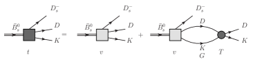
Figure 23: Diagrammatical interpretation of Eq. (107), in which $DK$ final state interaction is taken into account for the decay $\bar{B}^{0}_{s}\to D_{s}^{-}(DK)^{+}$. The dark square represents the amplitude $t$ for the process, in which the final state interaction is already taken into account. The light square represents the bare vertex for the process, denoted by $v$. Finally, the circle represents the hadronic amplitude for the elastic $DK$ scattering.

The hadronization of the $c\bar{s}$ pair proceeds then through the matrix element $\left(M^{2}\right)_{43}$, which in terms of mesons reads:

$$(\phi^{2})_{43}=K^{+}D^{0}+K^{0}D^{+}+\cdots~{},$$ (106)

where only terms containing a $KD$ pair are retained, since coupled channels are not considered here. We note that this $KD$ combination has $I=0$, as it should, since it is produced from a $c\bar{s}$, which has $I=0$, and the strong interaction hadronization conserves isospin.

Let $t$ be the full amplitude for the process $B^{0}_{s}\to D_{s}^{-}(DK)^{+}$, which already takes into account the final state interaction of the $DK$ pair. Also, let us denote by $v$ the bare vertex for the same reaction. To relate $t$ and $v$, that is, to take into account the final state interaction of the $DK$ pair, as sketched in Fig. 23, we write:

$$t=v+vG(s)T(s)=v(1+G(s)T(s))~{}.$$ (107)

From Eq. (80), the previous equation can also be written as:

$$t=v\frac{T(s)}{V(s)}~{}.$$ (108)

Because of the presence of the bound state below threshold, this amplitude will depend strongly on $s$ in the kinematical window ranging from threshold to $100\ \text{MeV}$ above it. Hence, the differential width for the process under consideration is given by:

$$\frac{\text{d}\Gamma}{d\sqrt{s}}=\frac{1}{32\pi^{3}M_{\bar{B}^{0}_{s}}^{2}}p_{D_{s}^{-}}\tilde{p}_{K}\left\lvert t\right\rvert^{2}=\mathcal{C}p_{D_{s}^{-}}\tilde{p}_{K}\left\lvert\frac{T(s)}{V(s)}\right\rvert^{2}~{},$$ (109)

where the bare vertex $v$ has been absorbed in $\mathcal{C}$, a global constant, and where $p_{D^{-}_{s}}$ is the momentum of the $D_{s}^{-}$ meson in the rest frame of the decaying $\bar{B}^{0}_{s}$ and $\tilde{p}_{K}$ the momentum of the kaon in the rest frame of the $DK$ system.

9.2 Results

	Central Value	$5\ \%$	$10\ \%$
$10^{3}\ \alpha\ (\text{GeV}^{-2})$	$2.06$	${}^{+0.17}_{-0.40}$	${}^{+0.10}_{-1.09}$
$M_{D^{\ast}_{s0}}\ (\text{MeV})$	$2317$	${}^{+14}_{-24}$	${}^{+21}_{-73}$
$a(\mu)$	$-1.30$	${}^{+0.15}_{-0.37}$	${}^{+0.27}_{-0.49}$
$|g|\ (\textrm{GeV})$	$11.0$	${}^{+1.0}_{-0.6}$	${}^{+2.2}_{-1.1}$
$a_{0}\ (\textrm{fm})$	$-1.0$	${}^{+0.2}_{-0.2}$	${}^{+0.4}_{-0.5}$
$r_{0}\ (\textrm{fm})$	$-0.14$	${}^{+0.06}_{-0.03}$	${}^{+0.16}_{-0.04}$
$P_{DK}$	$0.75$	${}^{+0.07}_{-0.06}$	${}^{+0.16}_{-0.11}$

Table 2: Fitted parameters ($\alpha$, $M_{D_{s0}^{\ast+}}$ and $a(\mu)$) and predicted quantities ($|g|$, $a_{0}$, $r_{0}$, $P_{DK}$) for $\mu=1.5\ \text{GeV}$. The second column shows the central value of the fit, whereas the third (fourth) column presents the errors (estimated by means of MC simulation) when the experimental error is 5% (10%).

We want to investigate the influence of the $D_{s0}^{\ast+}(2317)$ state in the $(DK)^{+}$ scattering amplitude. For this purpose, we generate synthetic data from our theory for the differential decay width for the process with Eqs. (109) and (90). We generate 10 synthetic points in a range of $100\ \text{MeV}$ starting from threshold, using the input discussed above and assuming $5\%$ or $10\%$ error. The idea is to use now these generated points as if they where experimental data and perform the inverse analysis to obtain information on the $D_{s0}^{\ast+}(2317)$.

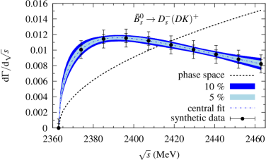
Figure 24: Differential decay width for the reaction $\bar{B}^{0}_{s}\to D^{-}_{s}(DK)^{+}$. The synthetic data (generated as explained in the text) are shown with black points. The smaller (larger) error bars correspond to a 5% (10%) experimental error. The dash-dotted line represents the theoretical prediction obtained with the central values of the fit. The light (dark) bands correspond to the estimation of the error (by means of a MC simulation) when fitting the data with 5% (10%) experimental error. The dashed line corresponds to a phase space distribution normalized to the same area in the range examined.

The generated synthetic data are shown in Fig. 24. As explained, we consider two different error bars, the smaller one corresponding to 5% experimental error and the larger one to 10%. A phase space distribution (i.e., a differential decay width proportional to $p_{D_{s}^{-}}p_{K}$, but with no other kinematical dependence of dynamical origin) is also shown in the figure (dashed line). The first important information extracted from the figure is that the data are clearly incompatible with the phase space distribution. This points to the presence of a resonant or bound state below threshold. Two error bands are shown in the same figure, the lighter and smaller (darker and larger) one corresponding to 5% (10%) experimental error. The fitted parameters ($a(\mu)$, $M_{D_{s0}^{\ast+}}$, and $\alpha$) are shown in Table 2. We also show the masses obtained and, by looking at the upper error, we observe that experimental data with a 10% error, which is clearly feasible with nowadays experimental facilities, can clearly determine the presence of a bound $DK$ state, corresponding to the $D_{s0}^{\ast}(2317)$, from the $DK$ distribution.

We can also determine $P_{DK}$, the probability of finding the $DK$ channel in the $D_{s0}^{\ast+}(2317)$ wave function. It is shown in the last row of Table 2. The central value $P_{DK}=0.75$ is the same as the initial one, but we are here interested in the errors, which are small enough even in the case of a 10% experimental error. This means that with the analysis of such an experiment one could address with enough accuracy the question of the molecular nature of the state ($D_{s0}^{\ast+}(2317)$, in this case).

Finally, it is also possible to determine other parameters related with $DK$ scattering, such as the scattering length ($a_{0}$) and the effective range ($r_{0}$). They are also shown in Table 2. They are compatible with the lattice QCD studies presented in Refs. Lang:2014yfa,Torres:2014vna. Namely, the results from Ref. Torres:2014vna are shown in Eqs. (93), and their mutual compatibility is clear.

10 Predictions for the $\bar{B}^{0}\to\bar{K}^{*0}X(YZ)$ and $\bar{B}^{0}_{s}\to\phi X(YZ)$ with $X(4160)$, $Y(3940)$, $Z(3930)$

The $XYZ$ resonances with masses in the region around 4000 MeV have posed a challenge to the common wisdom of mesons as made from $q\bar{q}$. There has been intense experimental work done at the BABAR, BELLE, CLEO, BES and other collaborations, and many hopes are placed in the role that the future FAIR facility with the PANDA collaboration and J-PARC will play in this field. There are early experimental reviews on the topic [169, 170, 171, 172] and more recent ones [173, 174, 175, 176, 177]. From the theoretical point of view there has also been an intensive activity trying to understand these states. There are quark model pictures [178, 179] and explicit tetraquark structures [180]. Molecular interpretations have also been given [181, 182, 183, 184, 185, 186, 187, 188, 189]. The introduction of heavy quark spin symmetry (HQSS) [190, 191, 192] has brought new light into the issue. QCD sum rules have also made some predictions [193, 194, 195]. Strong decays of these resonances have been studied to learn about the nature of these states [196, 197], while very often radiative decays are invoked as a tool to provide insight into this problem [198, 199, 200, 201, 202], although there might be exceptions[203]. It has even been speculated that some states found near thresholds of two mesons could just be cusps, or threshold effects [204]. However, this speculation was challenged in Ref. Guo:2014iya which showed that the near threshold narrow structures cannot be simply explained by kinematical threshold cusps in the corresponding elastic channels but require the presence of $S$-matrix poles. Along this latter point one should also mention a recent work on possible effects of singularities on the opposite side of the unitary cut enhancing the cusp structure for states with mass above a threshold [206]. Some theoretical reports on these issues can be found in other works[207, 208, 209].

So far, in the study of these $B$ decays the production of $XYZ$ states has not yet been addressed and we show below some reactions where these states can be produced, evaluating ratios for different decay modes and estimating the absolute rates[210]. This should stimulate experimental work that can shed light on the nature of some of these controversial states.

10.1 Formalism

Following the formalism developed in the former sections, we plot in Fig. 25 the basic mechanism at the quark level for $\bar{B}^{0}_{s}(\bar{B}^{0})$ decay into a final $c\bar{c}$ and another $q\bar{q}$ pair.

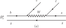
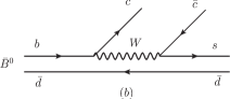
Figure 25: Diagrams at the quark level for $\bar{B}^{0}_{s}$ (a) and $\bar{B}^{0}$ (b) decays into $c\bar{c}$ and a $q\bar{q}$ pair.

The $c\bar{c}$ goes into the production of a $J/\psi$ and the $s\bar{s}$ or $s\bar{d}$ are hadronized to produce two mesons which are then allowed to interact to produce some resonant states. Here, we shall follow a different strategy and allow the $c\bar{c}$ to hadronize into two vector mesons, while the $s\bar{s}$ and $s\bar{d}$ will make the $\phi$ and $\bar{K}^{*0}$ mesons respectively. Let us observe that, apart for the $b\to c$ transition, most favored for the decay, we have selected an $s$ in the final state which makes the $c\to s$ transition Cabibbo allowed. This choice magnifies the decay rate, which should then be of the same order of magnitude as the $\bar{B}_{s}^{0}\to J/\psi f_{0}(980)$, which also had the same diagram at the quark level prior to the hadronization of the $s\bar{s}$ to produce two mesons.

In the next step, one introduces a new $q\bar{q}$ state with the quantum numbers of the vacuum, $\bar{u}u+\bar{d}d+\bar{s}s+\bar{c}c$, and see which combinations of mesons appear when added to $c\bar{c}$. This is depicted in Fig. 26. For this we follow the steps of the former section, and we have

$$c\bar{c}(\bar{u}u+\bar{d}d+\bar{s}s+\bar{c}c)\equiv(M\cdot M)_{44}\equiv(V\cdot V)_{44}$$ (110)

and

$$(V\cdot V)_{44}=D^{*0}\bar{D}^{*0}+D^{*+}D^{*-}+D^{*+}_{s}D^{*-}_{s}+J/\psi J/\psi.$$ (111)

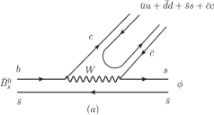
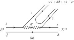
Figure 26: Hadronization of the $c\bar{c}$ pair into two vector mesons for $\bar{B}^{0}_{s}$ decay (a) and $\bar{B}^{0}$ decay (b).

Note that we have produced an $I=0$ combination, as it should be coming from $c\bar{c}$ and the strong interaction hadronization, given the isospin doublets ($D^{*+},-D^{*0}$), ($\bar{D}^{*0},\bar{D}^{*-}$). The $J/\psi J/\psi$ component is energetically forbidden and hence we can write

$$(V\cdot V)_{44}\to\sqrt{2}(D^{*}\bar{D}^{*})^{I=0}+D^{*+}_{s}D^{*-}_{s}.$$ (112)

The vector mesons produced undergo interaction and we use the work of Ref. Molina:2009ct, where an extension of the local hidden gauge approach[7, 8, 212, 9] is adopted, and where some $XYZ$ states are dynamically generated. Specifically, in Ref. Molina:2009ct four resonances were found, that are summarized in Table 3, together with the channel to which the resonance couples most strongly, and the experimental state to which they are associated.

Energy [MeV]	$I^{G}[J^{PC}]$	Strongest	Experimental
		channel	state
$3943-i7.4$	$0^{+}[0^{+~{}+}]$	$D^{*}\bar{D}^{*}$	$Y(3940)$ [213]
$3945-i0$	$0^{-}[1^{+~{}-}]$	$D^{*}\bar{D}^{*}$	? $Y_{P}$
$3922-i26$	$0^{+}[2^{+~{}+}]$	$D^{*}\bar{D}^{*}$	$Z(3930)$ [214]
$4169-i66$	$0^{+}[2^{+~{}+}]$	$D^{*}_{s}\bar{D}^{*}_{s}$	$X(4160)$ [215]

Table 3: States found in a previous work[211], the channel to which they couple most strongly, and the experimental states to which they are associated[171, 95]. $Y_{P}$ is a predicted resonance.

In Ref. Molina:2009ct, another state with $I=1$ was found, but this one cannot be produced with the hadronization of $c\bar{c}$. Some of these resonances have also been claimed to be of $D^{*}\bar{D}^{*}$ or $D^{*}_{s}\bar{D}^{*}_{s}$ molecular nature[199, 216, 181] using for it the Weinberg compositeness condition[161, 162, 168] and also using QCD sum rules[194, 217, 193], HQSS[191, 192] and phenomenological potentials[218].

The final state interaction of the $D^{*}\bar{D}^{*}$ and $D^{*}_{s}\bar{D}^{*}_{s}$ proceeds diagrammatically as depicted in Fig. 27. Starting from Eq. (112) the analytical expression for the formation of the resonance $R$ is given by

$$t(\bar{B}^{0}_{s}\to\phi R)=V_{P}(\sqrt{2}g_{D^{*}\bar{D}^{*},R}G_{D^{*}\bar{D}^{*}}+g_{D^{*}_{s}\bar{D}^{*}_{s},R}G_{D^{*}_{s}\bar{D}^{*}_{s}}),$$ (113)

where $G_{MM^{\prime}}$ is the loop function of the two intermediate meson propagators and $g_{MM^{\prime},R}$ is the coupling of the resonance to the $MM^{\prime}$ meson pair.

The formalism for $\bar{B}^{0}\to\bar{K}^{*0}R$ runs parallel since the hadronization procedure is identical, coming from the $c\bar{c}$, only the final state of $q\bar{q}$ is the $\bar{K}^{*0}$ rather than the $\phi$. Hence, the matrix element is identical to the one of $\bar{B}^{0}_{s}\to\phi R$, only the kinematics of different masses changes.

There is one more point to consider which is the angular momentum conservation. For $J^{P}_{R}=0^{+},2^{+}$, we have the transition $0^{-}\to J^{P}~{}1^{-}$. Parity is not conserved but the angular momentum is. By choosing the lowest orbital momentum $L$, we see that $L=0$ for $J^{P}=1^{+}$ and $L=1$ for $J^{P}=0^{+},2^{+}$. However, the dynamics will be different for $J^{P}=0^{+},1^{+},2^{+}$. This means that we can relate $\bar{B}^{0}_{s}\to Y(3940)\phi$ with $\bar{B}^{0}\to Y(3940)\bar{K}^{*0}$, $\bar{B}^{0}_{s}\to Z(3930)\phi$ with $\bar{B}^{0}\to Z(3930)\bar{K}^{*0}$, $\bar{B}^{0}_{s}\to X(4160)\phi$ with $\bar{B}^{0}\to X(4160)\bar{K}^{*0}$ and $\bar{B}^{0}_{s}\to Y_{P}\phi$ with $\bar{B}^{0}\to Y_{P}\bar{K}^{*0}$, but in addition we can relate $\bar{B}^{0}_{s}\to Z(3930)\phi$ with $\bar{B}^{0}_{s}\to X(4160)\phi$, and the same for $\bar{B}^{0}\to Z(3930)\bar{K}^{*0}$ with $\bar{B}^{0}\to X(4160)\bar{K}^{*0}$. Hence in this latter case we also have a $2^{+}$ state for both resonances and the only difference between them is the different coupling to $D^{*}\bar{D}^{*}$ and $D^{*}_{s}\bar{D}^{*}_{s}$, where the $Z(3930)$ couples mostly to $D^{*}\bar{D}^{*}$, while the $X(4160)$ couples mostly to $D^{*}_{s}\bar{D}^{*}_{s}$.

The partial decay width of these transitions is given by

$$\Gamma_{R_{i}}=\frac{1}{8\pi}\frac{1}{m^{2}_{\bar{B}_{i}^{0}}}\left|t_{\bar{B}_{i}^{0}\to\phi(\bar{K}^{*0})R_{i}}\right|^{2}P^{2L+1}_{\phi(\bar{K}^{*0})},$$ (114)

which allows us to obtain the following ratios, where the different unknown constants $V_{P}$, which summarize the production amplitude at tree level, cancel in the ratios:

$$R_{1}\equiv\frac{\Gamma_{\bar{B}^{0}_{s}\to\phi R^{J=0}}}{\Gamma_{\bar{B}^{0}\to K^{*0}R^{J=0}}},~{}~{}R_{2}\equiv\frac{\Gamma_{\bar{B}^{0}_{s}\to\phi R^{J=1}}}{\Gamma_{\bar{B}^{0}\to K^{*0}R^{J=1}}},R_{3}\equiv\frac{\Gamma_{\bar{B}^{0}_{s}\to\phi R^{J=2}_{1}}}{\Gamma_{\bar{B}^{0}\to K^{*0}R^{J=2}_{1}}},$$

$$R_{4}\equiv\frac{\Gamma_{\bar{B}^{0}_{s}\to\phi R^{J=2}_{2}}}{\Gamma_{\bar{B}^{0}\to K^{*0}R^{J=2}_{2}}},~{}~{}R_{5}\equiv\frac{\Gamma_{\bar{B}^{0}_{s}\to\phi R^{J=2}_{1}}}{\Gamma_{\bar{B}^{0}_{s}\to\phi R^{J=2}_{2}}},$$

where $R^{J=0}$, $R^{J=1}$, $R^{J=2}_{1}$ and $R^{J=2}_{2}$ are the $Y(3940)$, $Y_{P}$, $Z(3930)$ and $X(4160)$, respectively.

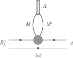
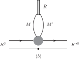
Figure 27: Diagrammatic representation of the formation of the resonances $R(X,Y,Z)$ through rescattering of $MM^{\prime}$ ($D^{*}\bar{D}^{*}$ or $D^{*}_{s}\bar{D}^{*}_{s}$) and coupling to the resonance.

10.2 Results

The couplings $g_{MM^{\prime},R}$ and the loop functions $G_{MM^{\prime}}$ in Eq. (113) are taken from Ref. Molina:2009ct, where the dimensional regularization was used to deal with the divergence of $G_{MM^{\prime}}$, fixing the regularization scale $\mu=1000$ MeV and the subtraction constant $\alpha=-2.07$. However, in Ref. Liang:2015twa some corrections to the work of Ref. Molina:2009ct are done, due to the findings of Ref. Liang:2014eba concerning heavy quark spin symmetry. It was found there that a factor $m_{D^{*}}/m_{K^{*}}$ has to be implemented in the hidden gauge coupling $g=m_{\rho}/2f_{\pi}$ in order to account for the $D^{*}\to D\pi$ decay. However, this factor should not be implemented in the Weinberg-Tomozawa terms (coming from exchange of vector mesons) because these terms automatically implement this factor in the vertices of vector exchange. In Ref. Liang:2015twa, $\mu=1000$ MeV and $\alpha=-2.19$ are used, by means of which a good reproduction of the masses is obtained.

We summarize here the results that we obtain for the ratios,

$$R_{1}=0.95,~{}~{}R_{2}=0.96,~{}~{}R_{3}=0.95,~{}~{}R_{4}=0.83,~{}~{}R_{5}=0.84.$$ (115)

As we can see, all the ratios are of the order of unity. The ratios close to unity for the $\phi$ or $K^{*0}$ production are linked to the fact that the resonances are dynamically generated from $D^{*}\bar{D}^{*}$ and $D^{*}_{s}\bar{D}^{*}_{s}$, which are produced by the hadronization of the $c\bar{c}$ pair. The ratio for the $J^{P}=2^{+}$ is even more subtle since it is linked to the particular couplings of these resonances to $D^{*}\bar{D}^{*}$ and $D^{*}_{s}\bar{D}^{*}_{s}$, which are a consequence of the dynamics that generates these states. Actually, the ratios $R_{1},~{}R_{2},~{}R_{3},~{}R_{4}$ are based only on phase space and result from the elementary mechanisms of Fig 25. One gets the same ratios as far as the resonances are $c\bar{c}$ based. Hence, even if these ratios do not prove the molecular nature of the resonances, they already provide valuable information telling us that they are $c\bar{c}$ based.

The ratio $R_{5}$ provides more information since it involves two independent resonances and it is not just a phase space ratio. If we take into account only phase space, then $R_{5}\approx 4$ instead of the value $0.84$ that we obtain.

As for the absolute rates, an analogy is established with the $\bar{B}^{0}_{s}\to J/\psi f_{0}(980)$ decay in Ref. Liang:2015twa, and branching fractions of the order of $10^{-4}$ are obtained, which are an order of magnitude bigger than many rates of the order of $10^{-5}$ already catalogued in the PDG [95].

Given the fact that the ratios $R_{1},~{}R_{2},~{}R_{3},~{}R_{4}$ obtained are not determining the molecular nature of the resonances, but only on the fact that they are $c\bar{c}$ based, a complementary test is proposed in the next section.

10.3 Complementary test of the molecular nature of the resonances

In this section we propose a test that is linked to the molecular nature of the resonances. We study the decay $\bar{B}^{0}_{s}\to\phi D^{*}\bar{D}^{*}$ or $\bar{B}^{0}_{s}\to\phi D_{s}^{*}\bar{D}_{s}^{*}$ close to the $D^{*}\bar{D}^{*}$ and $D_{s}^{*}\bar{D}_{s}^{*}$ thresholds.

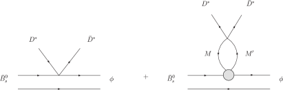
Figure 28: Feynman diagrams for the $D^{*}D^{*}$ production in $B^{0}_{s}$ decays.

Let us now look to the process $\bar{B}^{0}_{s}\to\phi D^{*}\bar{D}^{*}$ depicted in Fig. 28. The production matrix for this process will be given by

$$t_{(\bar{B}^{0}_{s}\to\phi D^{*}\bar{D}^{*})}=V_{P}(\sqrt{2}+\sqrt{2}\,G_{1}\,t_{(1\to 1)}+G_{2}\,t_{(2\to 1)})~{},$$ (116)

where $1$ and $2$ stands for the $D^{*}\bar{D}^{*}$ and $D^{*}_{s}\bar{D}^{*}_{s}$ channels, respectively. The differential cross section for production will be given by[47]:

$$\frac{d\Gamma}{dM_{\mathrm{inv}}}=\frac{1}{32\,\pi^{3}M^{2}_{\bar{B}^{0}_{s}}}p_{\phi}\tilde{p}_{D^{*}}|t_{(\bar{B}^{0}_{s}\to\phi D^{*}D^{*})}|^{2}p^{2L}_{\phi},$$ (117)

where $p_{\phi}$ is the $\phi$ momentum in the $\bar{B}^{0}_{s}$ rest frame and $\tilde{p}_{D^{*}}$ the $D^{*}$ momentum in the $D^{*}\bar{D}^{*}$ rest frame. By comparing this equation with Eq. (114) for the coalescence production of the resonance in $\bar{B}^{0}_{s}\to\phi~{}R$, we find

$$R_{\Gamma}=\frac{M^{3}_{R}}{p_{\phi}\tilde{p}_{D^{*}}}\frac{1}{\Gamma_{R}}\frac{d\Gamma}{dM_{\mathrm{inv}}}=\frac{M^{3}_{R}}{4\pi^{2}}\frac{p_{\phi}^{2L}(M_{\mathrm{inv}})}{p_{\phi}^{2L+1}(M_{R})}\left|\frac{t_{(\bar{B}^{0}_{s}\to\phi D^{*}\bar{D}^{*})}}{t_{(\bar{B}^{0}\to R\phi)}}\right|^{2},$$ (118)

where we have divided the ratio of widths by the phase space factor $p_{\phi}\tilde{p}_{D^{*}}$ and multiplied by $M_{R}^{3}$ to get a constant value at threshold and a dimensionless magnitude. We apply this method for the three resonances that couple strongly to $D^{*}\bar{D}^{*}$ (see Table 3). In the case of the resonance $R_{2}$ with $J=2$, that couples mostly to the $D^{*}_{s}\bar{D}^{*}_{s}$ channel (see Table 3), we look instead for the production of $D^{*}_{s}\bar{D}^{*}_{s}$, for which we have:

$$t_{(\bar{B}^{0}_{s}\to\phi D^{*}_{s}\bar{D}^{*}_{s})}=V_{P}(1+\sqrt{2}\,G_{1}\,t_{(1\to 2)}+G_{2}\,t_{(2\to 2)})~{},$$ (119)

and we use Eq. (118) but with $D^{*}_{s}\bar{D}^{*}_{s}$ instead of $D^{*}\bar{D}^{*}$ in the final state. Equation (118) is then evaluated using the scattering matrices obtained in Ref. Molina:2009ct modified as discussed above, together with Eqs. (116) and (119). The results are shown in Fig. 29.

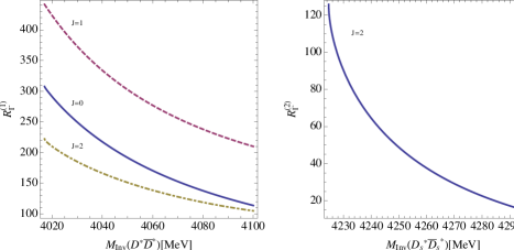
Figure 29: Results of $R_{\Gamma}^{(1)}$ of Eq. (118) as a function of $M_{inv}(D^{*}\bar{D}^{*})$ for the first three resonances of the Table 3 (left) and $R^{(2)}_{\Gamma}$ as a function of $M_{inv}(D_{s}^{*}\bar{D}_{s}^{*})$ (right) for the fourth resonance of the Table 3.

We can see that the ratios are different for each case and have some structure. We observe that there is a fall down of the differential cross sections as a function of energy, as it would correspond to the tail of a resonance below threshold. Note also that in the case of $D^{*}\bar{D}^{*}$, one produces the $I=0$ combination. If instead, one component like $D^{*+}D^{*-}$ is observed, the rate should be multiplied by $1/2$. In the case of $D^{*}_{s}\bar{D}^{*}_{s}$ there is a single component and the rate predicted is fine.

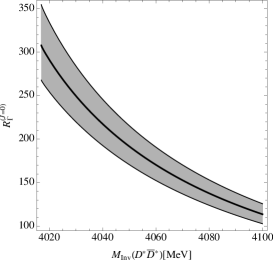
Figure 30: Results of $R_{\Gamma}^{(1)}$ of Eq. (118) as a function of $M_{inv}(D^{*}\bar{D}^{*})$ for spin$=0$.

11 Testing the molecular nature of ${D_{s0}^{\ast}(2317)}$ and ${D_{0}^{\ast}(2400)}$ in semileptonic ${B_{s}}$ and $B$ decays

In this section and the following one, we describe two processes for semileptonic decay, one for $B$ decay and the other for $D$ decay. The semileptonic $B$ decays will be used to test the molecular nature of the ${D_{s0}^{\ast}(2317)}$ and ${D_{0}^{\ast}(2400)}$, while those of the $D$ mesons, to be studied in section 12, will be used to further investigate the nature of scalar and vector mesons.

11.1 Introduction: semileptonic $B$ decays

The formalism is very similar to the one presented in former sections for nonleptonic $B$ decays. The basic mechanisms are depicted in Figs. 31, 32, 33. In all of them, after the $W$ emission one has a $c\bar{q}$ pair. In order to have two mesons in the final state the $c\bar{q}$ is allowed to hadronize into a pair of pseudoscalar mesons and the relative weights of the different pairs of mesons will be known. Once the meson pairs are produced they interact in the way described by the chiral unitary model in coupled channels, generating the $D_{s0}^{\ast}(2317)$ and $D_{0}^{\ast}(2400)$ resonances.

Figure 31: Semileptonic decay of $\bar{B}_{s}^{0}$ into $\bar{\nu}_{l}l^{-}$ and a primary $c\bar{s}$ pair.

Figure 32: Semileptonic decay of $\bar{B}^{0}$ into $\bar{\nu}_{l}l^{-}$ and a primary $c\bar{d}$ pair.

Figure 33: Semileptonic decay of $B^{-}$ into $\bar{\nu}_{l}l^{-}$ and a primary $c\bar{u}$ pair.

We will consider the semileptonic $B$ decays into $D$ resonances in the following decay modes:

$$\begin{split}&\bar{B}_{s}^{0}\to D_{s0}^{\ast}(2317)^{+}\bar{\nu}_{l}l^{-},\\ &\bar{B}^{0}\to D_{0}^{\ast}(2400)^{+}\bar{\nu}_{l}l^{-},\\ &B^{-}\to D_{0}^{\ast}(2400)^{0}\bar{\nu}_{l}l^{-},\end{split}$$ (120)

where the lepton flavor $l$ can be $e$ and $\mu$. With respect to the former sections we have now a different dynamics which we discuss below, together with the hadronization process.

11.2 Semileptonic decay widths

The decay amplitude of $B\to\bar{\nu}l^{-}\text{hadron(s)}$, $T_{B}$, is given by:

$$-iT_{B}= \overline{u}_{l}i\frac{g_{\rm W}}{\sqrt{2}}\gamma^{\alpha}\frac{1-\gamma_{5}}{2}v_{\nu}\times\frac{-ig_{\alpha\beta}}{p^{2}-M_{W}^{2}}$$

$$\times\overline{u}_{c}i\frac{g_{\rm W}V_{bc}}{\sqrt{2}}\gamma^{\beta}\frac{1-\gamma_{5}}{2}u_{b}\times(-iV_{\rm had})~{},$$ (121)

where $u_{l}$, $v_{\nu}$, $u_{c}$, and $u_{b}$ are Dirac spinors corresponding to the lepton $l^{-}$, neutrino, charm quark, and bottom quark, respectively, $g_{\rm W}$ is the coupling constant of the weak interaction, $V_{bc}$ is the CKM matrix element, and $M_{W}$ is the $W$ boson mass. The factor $V_{\rm had}$ describes the hadronization process and it will be evaluated in the sections below. Ignoring the squared three-momentum of the $W$ boson ($p^{2}$) which is much smaller than $M_{W}^{2}$ in the $B$ decay process, the decay amplitude becomes

$$T_{B}= -i\frac{G_{\rm F}V_{bc}}{\sqrt{2}}L^{\alpha}Q_{\alpha}\times V_{\rm had},$$ (122)

where the Fermi coupling constant $G_{\rm F}\equiv g_{\rm W}^{2}/(4\sqrt{2}M_{W}^{2})$ is introduced, and we define the lepton and quark parts of the $W$ boson couplings as:

$$L^{\alpha}\equiv\overline{u}_{l}\gamma^{\alpha}(1-\gamma_{5})v_{\nu},\quad Q_{\alpha}\equiv\overline{u}_{c}\gamma_{\alpha}(1-\gamma_{5})u_{b},$$ (123)

respectively.

In the calculation of the decay widths, one needs the average and sum of $|T_{B}|^{2}$ over the polarizations of the initial-state quarks and final-state leptons and quarks. In terms of the amplitude in Eq. (122), one can obtain the squared decay amplitude as

$$\frac{1}{2}\sum_{\rm pol}|T_{B}|^{2}=\frac{|G_{\rm F}V_{bc}V_{\rm had}|^{2}}{4}\sum_{\rm pol}|L^{\alpha}Q_{\alpha}|^{2}$$ (124)

where the factor $1/2$ comes from the average of the bottom quark polarization. Finally with some algebra discussed in Ref. Navarra:2015iea one obtains the squared decay amplitude:

$$\frac{1}{2}\sum_{\rm pol}|T_{B}|^{2}=\frac{4|G_{\rm F}V_{bc}V_{\rm had}|^{2}}{m_{\nu}m_{l}m_{B}m_{R}}(p_{B}\cdot p_{\nu})(p_{R}\cdot p_{l}).$$ (125)

Using the above squared amplitude we can calculate the decay width. We will be interested in two types of decays: three-body decays, such as $\bar{B}_{s}^{0}\rightarrow D_{s0}^{+}\,\bar{\nu_{l}}\,l^{-}$, and four-body decays, such as $\bar{B}_{s}^{0}\rightarrow D^{+}\,K^{0}\,\bar{\nu_{l}}\,l^{-}$ and also for the similar $\bar{B}^{0}$ and $B^{-}$ initiated processes. As it will be seen, both decay types can be described by the amplitude $T_{B}$ with different assumptions for $V_{\rm had}$.

11.3 Hadronization

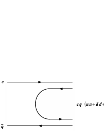
Figure 34: Schematic representation of the hadronization $c\bar{q}\to c\bar{q}\,(\bar{u}u+\bar{d}d+\bar{s}s+\bar{c}c)$.

For the conversion of quarks into hadrons in the final stage of hadron reactions we follow the same procedure as in former sections and assume that the matrix element for this process can be represented by an unknown constant. Explicit evaluations, where usually one must parametrize some information, have been discussed in subsection 3.3. Since the energies involved are of the order of a few GeV or less, this is a non-perturbative process. In some cases one can develop an approach based on effective Lagrangians[221, 222] to study hadronization. Here we describe hadronization as depicted in Fig. 34. An extra $\bar{q}q$ pair with the quantum numbers of the vacuum, $\bar{u}u+\bar{d}d+\bar{s}s+\bar{c}c$, is added to the already existing quark pair. The probability of producing the pair is assumed to be given by a number which is the same for all light flavors and which will cancel out when taking ratios of decay widths. We can write this $c\bar{q}\,(\bar{u}u+\bar{d}d+\bar{s}s+\bar{c}c)$ combination in terms of pairs of mesons. For this purpose we follow the procedure of the former sections and find the correspondence, with $\phi$ given by Eq. (105),

$$c\bar{s}\,(\bar{u}u+ \bar{d}d+\bar{s}s+\bar{c}c)\equiv\left(\phi\cdot\phi\right)_{43}$$

$$= D^{0}K^{+}+D^{+}K^{0}+D_{s}^{+}\left(-\frac{1}{\sqrt{3}}\eta+\sqrt{\frac{2}{3}}\eta^{\prime}\right)+\eta_{c}D_{s}^{+}~{},$$ (126)

$$c\bar{d}\,(\bar{u}u+ \bar{d}d+\bar{s}s+\bar{c}c)\equiv\left(\phi\cdot\phi\right)_{42}$$

$$= D^{0}\pi^{+}+D^{+}\left(-\frac{1}{\sqrt{2}}\pi^{0}+\frac{1}{\sqrt{3}}\eta+\frac{1}{\sqrt{6}}\eta^{\prime}\right)+D_{s}^{+}\bar{K}^{0}+\eta_{c}D^{+}~{},$$ (127)

$$c\bar{u}\,(\bar{u}u+ \bar{d}d+\bar{s}s+\bar{c}c)\equiv\left(\phi\cdot\phi\right)_{41}$$

$$= D^{0}\left(\frac{1}{\sqrt{2}}\pi^{0}+\frac{1}{\sqrt{3}}\eta+\frac{1}{\sqrt{6}}\eta^{\prime}\right)+D^{+}\pi^{-}+D_{s}^{+}K^{-}+\eta_{c}D^{0}~{}.$$ (128)

for $D_{s0}^{\ast}(2317)^{+}$, $D_{0}^{\ast}(2400)^{+}$, and $D_{0}^{\ast}(2400)^{0}$ production, respectively. As it was pointed out in Ref. Gamermann:2006nm, the most important channels for the description of $D_{s0}^{\ast}(2317)$ ($D_{0}^{\ast}(2400)$) are $DK$ and $D_{s}\eta$ ($D\pi$ and $D_{s}\bar{K}$). Therefore, the weights of the channels to generate the $D$ resonances can be written in terms of ket vectors as:

$$|(\phi\phi)_{43}\rangle =\sqrt{2}|DK(0,\,0)\rangle-\frac{1}{\sqrt{3}}|D_{s}\eta(0,\,0)\rangle~{},$$

$$|(\phi\phi)_{42}\rangle =-\sqrt{\frac{3}{2}}|D\pi(1/2,\,1/2)\rangle+|D_{s}\bar{K}(1/2,\,1/2)\rangle~{},$$ (129)

$$|(\phi\phi)_{41}\rangle =\sqrt{\frac{3}{2}}|D\pi(1/2,\,-1/2)\rangle-|D_{s}\bar{K}(1/2,\,-1/2)\rangle~{},$$

where we have used two-body states in the isospin basis, which are specified as $(I,\,I_{3})$. Due to the isospin symmetry, both the charged and neutral $D_{0}^{\ast}(2400)$ are produced with the weight of $|(\phi\phi)_{42}\rangle=-|(\phi\phi)_{41}\rangle$, which means that the ratio of the decay widths into the charged and neutral $D_{0}^{\ast}(2400)$ is almost unity. Using these weights, we can write $V_{\rm had}$ in terms of two pseudoscalars.

After the hadronization of the quark-antiquark pair, two mesons are formed and start to interact. The $D$ resonances can be generated as a result of complex two-body interactions with coupled channels described by the Bethe-Salpeter equation. If the resonance is formed, independently of how it decays, the process is usually called “coalescence” [223, 224] and it is a reaction with three particles in the final state (see Fig. 35). If we look for a specific two meson final channel we can have it by “prompt” or direct production (first diagram of Fig. 36), and by rescattering, generating the resonance (second diagram of Fig. 36). This process is usually called “rescattering” and it is a reaction with four particles in the final state. Coalescence and rescattering will be discussed in the next sections.

Figure 35: Diagrammatic representation of $D_{s0}^{\ast+}(2317)$ production via meson coalescence after rescattering.

Figure 36: Diagrammatic representation of $DK$ production: directly (on the left) and via rescattering (on the right) in $\bar{B}^{0}_{s}$ decays.

11.4 Coalescence

In this section we consider $D$ resonance production via meson coalescence as depicted in Fig. 35. This process has a three-body final state with a lepton, its neutrino and the resonance R. The hadronization factor, $V_{\rm had}$, can be written as

$$V_{\text{had}}(D_{s0}^{\ast}(2317)) = C\left(\sqrt{2}G_{DK}g_{DK}-\frac{1}{\sqrt{3}}G_{D_{s}\eta}g_{D_{s}\eta}\right),$$ (130)

$$V_{\text{had}}(D_{0}^{\ast}(2400)^{+}) = C\left(-\sqrt{\frac{3}{2}}G_{D\pi}g_{D\pi}+G_{D_{s}\bar{K}}g_{D_{s}\bar{K}}\right),$$ (131)

Here $g_{i}$ is the coupling constant of the $D$ resonance to the $i$-th two meson channel and $G_{i}$ is the loop function of two meson propagators. As mentioned above $V_{\text{had}}(D_{0}^{\ast}(2400)^{0})=-V_{\text{had}}(D_{0}^{\ast}(2400)^{+})$. We will assume that $C$ is a constant in the limited range of invariant masses that we discuss and hence it will be cancelled when we take the ratio of decay widths.

The formula for the width is then given by

$$\Gamma_{\rm coal}=\frac{|G_{\rm F}V_{bc}V_{\rm had}(D^{\ast})|^{2}}{8\pi^{3}m_{B}^{3}m_{R}}\int dM_{\rm inv}^{(\nu l)}p_{D}^{\rm cm}\tilde{p}_{\nu}[M_{\rm inv}^{(\nu l)}]^{2}\left(\tilde{E}_{B}\tilde{E}_{R}-\frac{\tilde{p}_{B}^{2}}{3}\right)~{},$$ (132)

where the integral range of $M_{\rm inv}^{(\nu l)}$ is $[m_{l}+m_{\nu},\,m_{B}-m_{R}]$. In Eq. (132), we have:

$$p_{D}^{\text{cm}} =\frac{\lambda^{1/2}\left(m_{B}^{2},\left[M_{\text{inv}}^{(\nu l)}\right]^{2},m_{R}^{2}\right)}{2m_{B}}~{},$$ (133)

$$\tilde{p}_{\nu} =\frac{\lambda^{1/2}\left(\left[M_{\text{inv}}^{(\nu l)}\right]^{2},m_{\nu}^{2},m_{l}^{2}\right)}{2m_{B}}~{},$$ (134)

$$\tilde{E}_{B} =\frac{m_{B}^{2}+\left[M_{\text{inv}}^{(\nu l)}\right]^{2}-m_{R}^{2}}{2M_{\text{inv}}^{(\nu l)}}~{},$$ (135)

$$\tilde{E}_{R} =\frac{m_{B}^{2}-\left[M_{\text{inv}}^{(\nu l)}\right]^{2}-m_{R}^{2}}{2M_{\text{inv}}^{(\nu l)}}~{},$$ (136)

where $\tilde{p}_{B}^{2}=\tilde{E}_{B}^{2}-m_{B}^{2}$. Here $m_{B}$ and $m_{R}$ are the masses of the $B$ and $D^{\ast}$ mesons, respectively. Further detailed can be found in Ref. Navarra:2015iea.

11.5 Rescattering

Now we address the production of two pseudoscalars with prompt production plus rescattering through a $D$ resonance, as depicted in the diagrams of Fig. 36. The hadronization amplitude $V_{\rm had}$ in the isospin basis is given by

$$V_{\text{had}}(DK) = C\left(\sqrt{2}+\sqrt{2}G_{DK}T_{DK\to DK}-\frac{1}{\sqrt{3}}G_{D_{s}\eta}T_{D_{s}\eta\to DK}\right),$$ (137)

$$V_{\text{had}}(D_{s}\eta) = C\left(-\frac{1}{\sqrt{3}}+\sqrt{2}G_{DK}T_{DK\to D_{s}\eta}-\frac{1}{\sqrt{3}}G_{D_{s}\eta}T_{D_{s}\eta\to D_{s}\eta}\right),$$ (138)

$$V_{\text{had}}(D\pi) = C\left(-\sqrt{\frac{3}{2}}-\sqrt{\frac{3}{2}}G_{D\pi}T_{D\pi\to D\pi}+G_{D_{s}\bar{K}}T_{D_{s}\bar{K}\to D\pi}\right),$$ (139)

$$V_{\text{had}}(D_{s}\bar{K}) = C\left(1-\sqrt{\frac{3}{2}}G_{D\pi}T_{D\pi\to D_{s}\bar{K}}+G_{D_{s}\bar{K}}T_{D_{s}\bar{K}\to D_{s}\bar{K}}\right).$$ (140)

As it can be seen, the prefactor $C$ is the same in all the reactions. In order to calculate decay widths in the particle basis, we need to multiply the amplitudes by the appropriate Clebsch-Gordan coefficients.

Using Eq. (125) we can compute the differential decay width $d\Gamma_{i}/dM_{\rm inv}^{(i)}$, where $i$ represents the two pseudoscalar states and $M_{\rm inv}^{(i)}$ is the invariant mass of the two pseudoscalars, as

$$\frac{d\Gamma_{i}}{dM_{\rm inv}^{(i)}}=\frac{|G_{\rm F}V_{bc}V_{\rm had}(i)|^{2}}{32\pi^{5}m_{B}^{3}M_{\rm inv}^{(i)}}\int dM_{\rm inv}^{(\nu l)}P^{\rm cm}\tilde{p}_{\nu}\tilde{p}_{i}[M_{\rm inv}^{(\nu l)}]^{2}\left(\tilde{E}_{B}\tilde{E}_{i}-\frac{\tilde{p}_{B}^{2}}{3}\right),$$ (141)

where $P^{\rm cm}$ is the momentum of the $\nu l$ system in the $B$ rest frame, $\tilde{p}_{\nu}$ is the momentum of the $\nu$ in the neutrino lepton rest system [given in Eq. (134)], and $\tilde{p}_{i}$ is the relative momentum of the two pseudoscalars in their rest frame.

11.6 The $DK$-$D_{s}\eta$ and $D\pi$ - $D_{s}\bar{K}$ scattering amplitudes

We will now discuss the meson-meson scattering amplitudes for the rescattering to generate the $D_{s0}^{\ast}(2317)$ and $D_{0}^{\ast}(2400)$ resonances in the final state of the $B$ decay. In Ref. Gamermann:2006nm it was found that the couplings to $DK$ and $D_{s}\eta$ are dominant for $D_{s0}^{\ast}(2317)$ and the couplings to $D\pi$ and $D_{s}\bar{K}$ are dominant for $D_{0}^{\ast}(2400)$. Therefore, in the following we concentrate on $DK$-$D_{s}\eta$ two-channel scattering in isospin $I=0$ and $D\pi$-$D_{s}\bar{K}$ two-channel scattering in $I=1/2$, extracting essential portions from Ref. Gamermann:2006nm and assuming isospin symmetry. Namely, we obtain these amplitudes by solving a coupled-channel scattering equation in an algebraic form

$$T_{ij}(s)=V_{ij}(s)+\sum_{k}V_{ik}(s)G_{k}(s)T_{kj}(s),$$ (142)

where $i$, $j$, and $k$ are channel indices, $s$ is the Mandelstam variable of the scattering, $V$ is the interaction kernel, and $G$ is the two-body loop function. This generalizes what was found in section 9 with just one channel.

The interaction kernel $V$ corresponds to the tree-level transition amplitudes obtained from phenomenological Lagrangians developed in Ref. Gamermann:2006nm. We use dimensional regularization in the loop function $G$.

The $D$ resonances can appear as poles of the scattering amplitude $T_{ij}(s)$ with the residue $g_{i}g_{j}$:

$$T_{ij}(s)=\frac{g_{i}g_{j}}{s-s_{\rm pole}}+(\text{regular at }s=s_{\rm pole}).$$ (143)

The pole is described by its position $s_{\rm pole}$ and the constant $g_{i}$, which is the coupling constant of the $D$ resonance to the $i$ channel. Further details can be found in Ref. Navarra:2015iea.

Let us introduce the concept of compositeness, which is defined as the contribution from the two-body part to the normalization of the total wave function and measures the fraction of the two-body state [225, 93, 94, 226, 168]. The expression of the compositeness is given by

$$X_{i}=-g_{i}^{2}\left[\frac{dG_{i}}{ds}\right]_{s=s_{\rm pole}}~{}.$$ (144)

In an analogous way we introduce the elementariness $Z$, which measures the fraction of missing channels and is expressed as

$$Z=-\sum_{i,j}g_{j}g_{i}\left[G_{i}\frac{dV_{ij}}{ds}G_{j}\right]_{s=s_{\rm pole}}~{}.$$ (145)

In general both the compositeness $X_{i}$ and elementariness $Z$ are complex values for a resonance state and hence one cannot interpret the compositeness (elementariness) as the probability to observe a two-body (missing-channel) component inside the resonance except for bound states. However, a striking property is that the sum of them is exactly unity:

$$\sum_{i}X_{i}+Z=1,$$ (146)

which is guaranteed by a generalized Ward identity proved in Ref. Sekihara:2010uz. Therefore one can deduce the structure by comparing the value of the compositeness with unity, on the basis of the similarity to the stable bound state case. The values of the compositeness and elementariness of the $D$ resonances in this approach are listed in Table 4. The result indicates that the $D_{s0}^{\ast}(2317)$ resonance, which is obtained as a bound state in the present model, is indeed dominated by the $DK$ component. This has been corroborated in the recent analysis of lattice QCD results of Ref. Torres:2014vna. In contrast, we may conclude that the $D_{0}^{\ast}(2400)$ resonance is constructed with missing channels, although the imaginary part for each component is not negligible.

$D_{s0}^{\ast}(2317)$			$D_{0}^{\ast}(2400)$
$\sqrt{s_{\rm pole}}$	$2317\text{ MeV}$		$\sqrt{s_{\rm pole}}$	$2128-160i\text{ MeV}$
$g_{DK}$	$10.58\text{ GeV}$		$g_{D\pi}$	$\phantom{-}9.00-6.18i\text{ GeV}$
$g_{D_{s}\eta}$	$-6.11\text{ GeV}~{}$		$g_{D_{s}\bar{K}}$	$-7.68+4.35i\text{ GeV}$
$X_{DK}$	$0.69$		$X_{D\pi}$	$0.34+0.41i$
$X_{D_{s}\eta}$	$0.09$		$X_{D_{s}\bar{K}}$	$0.03-0.12i$
$Z$	$0.22$		$Z$	$0.63-0.28i$

Table 4: Pole position $\sqrt{s_{\rm pole}}$, coupling constant $g_{i}$, compositeness $X_{i}$, and elementariness $Z$ for the $D$ resonances in the isospin basis.

11.7 Numerical results

$R$	$0.45$
$\Gamma_{B^{-}\to D_{0}^{\ast}(2400)^{0}\bar{\nu}_{l}l^{-}}/\Gamma_{\bar{B}^{0}\to D_{0}^{\ast}(2400)^{+}\bar{\nu}_{l}l^{-}}$	$1.00$
$\mathcal{B}[\bar{B}^{0}\to D_{0}^{\ast}(2400)^{+}\bar{\nu}_{l}l^{-}]$	$4.5\times 10^{-3}$ (input)
$\mathcal{B}[\bar{B}^{-}\to D_{0}^{\ast}(2400)^{0}\bar{\nu}_{l}l^{-}$]	$4.9\times 10^{-3}$

Table 5: Ratios of decay widths and branching fractions of semileptonic $B$ decays.

First we consider the coalescence case. The numerical results are summarized in Table 5. The most interesting quantity is the ratio $R=\Gamma_{\bar{B}_{s}^{0}\to D_{s0}^{\ast}(2317)^{+}\bar{\nu}_{l}l^{-}}/\Gamma_{\bar{B}^{0}\to D_{0}^{\ast}(2400)^{+}\bar{\nu}_{l}l^{-}}$ in the coalescence treatment, which removes the unknown factor $C$ of the hadronization process. The decay width in the coalescence is expressed by Eq. (132). The coupling constants of the two mesons to the $D$ resonances are listed in Table 4. Note that there are no fitting parameters for the ratio $R$ in this scheme. As a result, we obtain the ratio of the decay widths as $R=0.45$. On the other hand, we find that the ratio $\Gamma_{B^{-}\to D_{0}^{\ast}(2400)^{0}\bar{\nu}_{l}l^{-}}/\Gamma_{\bar{B}^{0}\to D_{0}^{\ast}(2400)^{+}\bar{\nu}_{l}l^{-}}$ is $1.00$, which can be expected from the same strength of the decay amplitude to the charged and neutral $D_{0}^{\ast}(2400)$ due to the isospin symmetry, as discussed after Eq. (129).

The absolute value of the common prefactor $C$ can be determined with the help of experimental data on the decay width. The branching fraction of the semileptonic decay $\bar{B}^{0}\to D_{0}^{\ast}(2400)^{+}\bar{\nu}_{l}l^{-}$ to the total decay is reported as $(4.5\pm 1.8)\times 10^{-3}$ by the Particle Data Group [95]. By using this mean value we find $C=7.22$, and the fractions of decays $\bar{B}_{s}^{0}\to D_{s0}^{\ast}(2317)^{+}\bar{\nu}_{l}l^{-}$ and $B^{-}\to D_{0}^{\ast}(2400)^{0}\bar{\nu}_{l}l^{-}$ to the total decay widths are obtained as $2.0\times 10^{-3}$ and $4.9\times 10^{-3}$, respectively. The values of these fractions are similar to each other. The difference of the fractions of $\bar{B}^{0}\to D_{0}^{\ast}(2400)^{+}\bar{\nu}_{l}l^{-}$ and $B^{-}\to D_{0}^{\ast}(2400)^{0}\bar{\nu}_{l}l^{-}$ comes from the fact that the total decay widths of $\bar{B}^{0}$ and $B^{-}$ are different.

Table 6: Branching fraction of the process $\bar{B}_{s}^{0}\to D_{s0}^{\ast}(2317)^{+}\bar{\nu}_{l}l^{-}$ in percentage

Approach	$\mathcal{B}[\bar{B}_{s}^{0}\to D_{s0}^{\ast}(2317)^{+}\bar{\nu}_{l}l^{-}]$
This work	$0.20$
QCDSR + HQET [228]	$0.09-0.20$
QCDSR (SVZ) [229]	$0.10$
LCSR [230]	$0.23\pm 0.11$
CQM [231]	$0.49-0.57$
CQM [232]	$0.44$
CQM [233]	$0.39$

A comparison of our predictions for $\mathcal{B}[\bar{B}_{s}^{0}\to D_{s0}^{\ast}(2317)^{+}\bar{\nu}_{l}l^{-}]$ with the results obtained with other approaches is presented in Table 6. We emphasize that our approach is the only one where the $D_{s0}^{\ast}(2317)^{+}$ is treated as a mesonic molecule. Looking at Table 6 we can divide the results in two groups: the first four numbers, which are “small” and the last three, which are “large”. In the second group, the constituent quark models (CQM) yield larger branching fractions. In Ref. Navarra:2015iea one can find some discussion on the origin of the differences based on the compact picture of the quark models versus the more extended structure of the molecular description.

Now let us discuss the rescattering process for the final-state two mesons. We keep using the common prefactor $C=7.22$ fixed from the experimental value of the width of the semileptonic decay $\bar{B}^{0}\to D_{0}^{\ast}(2400)^{+}\bar{\nu}_{l}l^{-}$. The meson-meson scattering amplitude was discussed in Sec. 11.6, and now we include the $D_{s}\pi^{0}$ channel as the isospin-breaking decay mode of $D_{s0}^{\ast}(2317)$. Namely, we calculate the scattering amplitude involving the $D_{s}\pi^{0}$ channel as

$$T_{i\to D_{s}\pi^{0}}=\frac{g_{i}g_{D_{s}\pi^{0}}}{s-[M_{D_{s0}^{\ast}}-i\Gamma_{D_{s0}^{\ast}}/2]^{2}},$$ (147)

for $i=DK$ and $D_{s}\eta$. We take the $D_{s0}^{\ast}(2317)$ mass as $M_{D_{s0}^{\ast}}=2317\text{ MeV}$, while we assume its decay width as $\Gamma_{D_{s0}^{\ast}}=3.8\text{ MeV}$, which is the upper limit from experiments [95]. The $D_{s0}^{\ast}(2317)$-$i$ coupling constant $g_{i}$ ($i=DK$, $D_{s}\eta$) is taken from Table 4, and the $D_{s0}^{\ast}(2317)$-$D_{s}\pi^{0}$ coupling constant $g_{D_{s}\pi^{0}}$ is calculated from the $D_{s0}^{\ast}(2317)$ decay width as

$$g_{D_{s}\pi^{0}}=\sqrt{\frac{8\pi M_{D_{s0}^{\ast}}^{2}\Gamma_{D_{s0}^{\ast}}}{p_{\pi}}},$$ (148)

with the pion center-of-mass momentum $p_{\pi}$, and we obtain $g_{D_{s}\pi^{0}}=1.32$ GeV.

Figure 37: Differential decay width $d\Gamma_{i}/dM_{\rm inv}^{(i)}$ for the two pseudoscalars channel $i$ in the isospin basis. Here we consider the semileptonic decays $\bar{B}_{s}^{0}\to(DK)^{+}\bar{\nu}_{l}l^{-}$, $(D_{s}\pi^{0})^{+}\bar{\nu}_{l}l^{-}$ and $\bar{B}^{0}\to(D\pi)^{+}\bar{\nu}_{l}l^{-}$. The $DK$ and $D_{s}\pi^{0}$ channels couple to the $D_{s0}^{\ast}(2317)^{+}$ resonance, and $D\pi$ to the $D_{0}^{\ast}(2400)$ resonance. The peak height for the $D_{s}\pi^{0}$ channel is $d\Gamma_{D_{s}\pi^{0}}/dM_{\rm inv}^{(D_{s}\pi^{0})}\sim 1.5\cdot 10^{-13}$.

In Fig. 37 we show our predictions for the differential decay width $d\Gamma_{i}/dM_{\rm inv}^{(i)}$ (Eq. (141)), where $i$ represents the two pseudoscalar states. In the figure we use the isospin basis. When translating into the particle basis we use the following relations:

$$[D^{0}K^{+}]=[D^{+}K^{0}]=\frac{1}{2}[DK],$$ (149)

$$[D_{s}^{+}\pi^{0}]=[D_{s}\pi^{0}],$$ (150)

$$[D^{0}\pi^{+}]=2[D^{+}\pi^{0}]=\frac{2}{3}[D\pi],$$ (151)

where $[AB]$ is the partial decay width to the $AB$ channel. An interesting point is that the $DK$ mode shows a rapid increase from its threshold $\approx 2360\text{ MeV}$ due to the existence of the bound state, i.e., the $D_{s0}^{\ast}(2317)$ resonance. In experiments, such a rapid increase from the $DK$ threshold would support the interpretation of the $D_{s0}^{\ast}(2317)$ resonance as a $DK$ bound state. The strength of the $DK$ contribution in the $M_{\rm inv}^{(i)}\gtrsim 2.4\text{ GeV}$ region is similar to that of $D\pi$, which corresponds to the “tail” for the $D_{0}^{\ast}(2400)$ resonance. On the other hand, the $D_{s}\pi^{0}$ peak coming from the $D_{s0}^{\ast}(2317)$ resonance is very sharp due to its narrow width.

The distributions shown in Fig. 37 are our predictions and they can be measured at the LHCb. They were obtained in the framework of the chiral unitary approach in coupled channels and their experimental observation would give support to the $D_{s0}^{\ast}(2317)$ and $D_{0}^{\ast}(2400)$ as dynamically generated resonances, which is inherent to this approach.

Apart from comparing shapes and relative strength, one can make an analysis of the $DK$ mass distribution as suggested in Ref. Albaladejo:2015kea to determine $g_{DK}$. With this value and the use of Eq. (144) one can determine the amount of $DK$ component in the $D_{s0}^{\ast}(2317)$ wave function. Note that the shape of the $DK$ mass distribution is linked to the potential, with its associated energy dependence, and the mass of the $D_{s0}^{\ast}(2317)$ [166]. With the same binding of the resonance, different models that have different amount of $DK$ component provide different shapes, leading to different values of the $g_{DK}$ coupling, and it is possible to discriminate among models that have a different nature for the $D_{s0}^{\ast}(2317)$ resonance.

12 Investigating the nature of light scalar mesons with semileptonic decays of $D$ mesons

Figure 38: (a) Semileptonic decay of $D^{+}_{s}$ into $l^{+}\nu_{l}$ and a primary $s\bar{s}$ pair. (b) Semileptonic decay of $D^{+}_{s}$ into $l^{+}\nu_{l}$ and two pseudoscalar mesons $P$ with a hadronization.

Here we consider the semileptonic decay of $D\to\text{hadron(s)}+l^{+}\nu_{l}$, extending the work reported in the former section. The semileptonic $D$ decays have been experimentally investigated in, e.g., BES [234, 235], FOCUS [236, 237], BaBar [238, 239], and CLEO [240, 241, 242, 243, 244]. In order to see how the semileptonic decay takes place, let us consider the $D_{s}^{+}$ meson. Since the constituent quark component of $D_{s}^{+}$ is $c\bar{s}$, we expect a Cabibbo favored semileptonic decay of $c\to s\,l^{+}\,\nu_{l}$ and hence the decay $D_{s}^{+}\to(s\bar{s})\,l^{+}\,\nu_{l}$ with $s\bar{s}$ being the vector meson $\phi(1020)$, which is depicted in Fig. 38(a). Actually this semileptonic decay mode has been observed in experiments, and its branching fraction to the total decay width is $\mathcal{B}[D_{s}^{+}\to\phi(1020)\,e^{+}\,\nu_{e}]=2.49\pm 0.14\%$ [95] (see Table 7, in which we list branching fractions for the semileptonic decays of $D_{s}^{+}$, $D^{+}$, and $D^{0}$ reported by the Particle Data Group). In this study we consider the production of the $f_{0}(980)$ or $f_{0}(500)$ as dynamically generated resonances in the semileptonic $D_{s}^{+}$ decay, so we have to introduce an extra $\bar{q}q$ pair to make a hadronization as shown in Fig. 38(b).

Table 7: Branching fractions for the semileptonic decays of $D_{s}^{+}$, $D^{+}$, and $D^{0}$ reported by the Particle Data Group [95]. In this Table we only show decay modes relevant to this study.

$D_{s}^{+}$
Mean life [s]	$(500\pm 7)\times 10^{-15}$
$\mathcal{B}[\phi(1020)e^{+}\nu_{e}]$	$(2.49\pm 0.14)\times 10^{-2}$
$\mathcal{B}[\omega(782)e^{+}\nu_{e}]$	$<2.0\times 10^{-3}$
$\mathcal{B}[K^{\ast}(892)^{0}e^{+}\nu_{e}]$	$(1.8\pm 0.7)\times 10^{-3}$
$\mathcal{B}[f_{0}(980)e^{+}\nu_{e},\,f_{0}(980)\to\pi^{+}\pi^{-}]$	$(2.00\pm 0.32)\times 10^{-3}$
$D^{+}$
Mean life [s]	$(1040\pm 7)\times 10^{-15}$
$\mathcal{B}[\bar{K}^{\ast}(892)^{0}e^{+}\nu_{e},\,\bar{K}^{\ast}(892)^{0}\to K^{-}\pi^{+}]$	$(3.68\pm 0.10)\times 10^{-2}$
$\mathcal{B}[(K^{-}\pi^{+})_{s\text{-wave}}e^{+}\nu_{e}]$	$(2.32\pm 0.10)\times 10^{-3}$
$\mathcal{B}[\bar{K}^{\ast}(892)^{0}\mu^{+}\nu_{\mu},\,\bar{K}^{\ast}(892)^{0}\to K^{-}\pi^{+}]$	$(3.52\pm 0.10)\times 10^{-2}$
$\mathcal{B}[\rho(770)^{0}e^{+}\nu_{e}]$	$(2.18^{+0.17}_{-0.25})\times 10^{-3}$
$\mathcal{B}[\rho(770)^{0}\mu^{+}\nu_{\mu}]$	$(2.4\pm 0.4)\times 10^{-3}$
$\mathcal{B}[\omega(782)e^{+}\nu_{e}]$	$(1.82\pm 0.19)\times 10^{-3}$
$\mathcal{B}[\phi(1020)e^{+}\nu_{e}]$	$<9\times 10^{-5}$
$D^{0}$
Mean life [s]	$(410.1\pm 1.5)\times 10^{-15}$
$\mathcal{B}[K^{\ast}(892)^{-}e^{+}\nu_{e}]$	$(2.16\pm 0.16)\times 10^{-2}$
$\mathcal{B}[K^{\ast}(892)^{-}\mu^{+}\nu_{\mu}]$	$(1.90\pm 0.24)\times 10^{-2}$
$\mathcal{B}[K^{-}\pi^{0}e^{+}\nu_{e}]$	$(1.6^{+1.3}_{-0.5})\times 10^{-2}$
$\mathcal{B}[\bar{K}^{0}\pi^{-}e^{+}\nu_{e}]$	$(2.7^{+0.9}_{-0.7})\times 10^{-2}$
$\mathcal{B}[\rho(770)^{-}e^{+}\nu_{e}]$	$(1.9\pm 0.4)\times 10^{-3}$

12.1 Formulation

$D_{s}^{+}$
$\phi(1020)\,l^{+}\,\nu_{l}$	favored
$K^{\ast}(892)^{0}\,l^{+}\,\nu_{l}$	suppressed
$\pi^{+}\pi^{-}\,l^{+}\,\nu_{l}$	favored
$K^{+}K^{-}\,l^{+}\,\nu_{l}$	favored
$\pi^{-}K^{+}\,l^{+}\,\nu_{l}$	suppressed
$D^{+}$
$\bar{K}^{\ast}(892)^{0}\,l^{+}\,\nu_{l}$	favored
$\rho(770)^{0}\,l^{+}\,\nu_{l}$	suppressed
$\omega(782)\,l^{+}\,\nu_{l}$	suppressed
$\pi^{+}\pi^{-}\,l^{+}\,\nu_{l}$	suppressed
$\pi^{0}\eta\,l^{+}\,\nu_{l}$	suppressed
$K^{+}K^{-}\,l^{+}\,\nu_{l}$	suppressed
$\pi^{+}K^{-}\,l^{+}\,\nu_{l}$	favored
$D^{0}$
$K^{\ast}(892)^{-}\,l^{+}\,\nu_{l}$	favored
$\rho(770)^{-}\,l^{+}\,\nu_{l}$	suppressed
$\pi^{-}\eta\,l^{+}\,\nu_{l}$	suppressed
$K^{0}K^{-}\,l^{+}\,\nu_{l}$	suppressed
$\pi^{-}\bar{K}^{0}\,l^{+}\,\nu_{l}$	favored

Table 8: Semileptonic decay modes of $D_{s}^{+}$, $D^{+}$, and $D^{0}$ considered in this study. The lepton flavor $l$ is $e$ and $\mu$. We also specify Cabibbo favored/suppressed process for each decay mode; the semileptonic decay into two pseudoscalar mesons is classified following the discussions given in Sec. 12.3.

In this section we formulate the semileptonic decay widths of $D_{s}^{+}$, $D^{+}$, and $D^{0}$ into light scalar and vector mesons:

$$D_{s}^{+},\,D^{+},\,D^{0}\to\begin{cases}Sl^{+}\nu_{l},\quad S\to PP,\\ Vl^{+}\nu_{l},\end{cases}$$ (152)

where $S$, $V$, and $P$ represent the light scalar, vector, and pseudoscalar mesons, respectively, and the lepton flavor $l$ can be $e$ and $\mu$. Explicit decay modes are listed in Table 8.

12.2 Amplitudes and widths of semileptonic $D$ decays

The calculation of the amplitudes proceeds exactly like in the former section changing the masses and the coefficient $C$.

12.3 Hadronizations

Figure 39: Diagrammatic representation of the direct plus rescattering processes for two pseudoscalar mesons. The solid and dashed lines denote quarks and pseudoscalar mesons, respectively. The shaded ellipses indicate the hadronization of a quark–antiquark pair into two pseudoscalar mesons, while the open circle indicates the rescattering of two pseudoscalar mesons.

Next we fix the mechanism for the appearance of the scalar and vector mesons in the final state of the semileptonic decay. We note that, for the scalar and vector mesons in the final state, the hadronization processes should be different from each other according to their structure. For the scalar mesons, we employ the chiral unitary approach, in which the scalar mesons are dynamically generated from the interaction of two pseudoscalar mesons governed by the chiral Lagrangians. Therefore, in this picture the light quark–antiquark pair after the $W$ boson emission gets hadronized by adding an extra $\bar{q}q$ with the quantum number of the vacuum, $\bar{u}u+\bar{d}d+\bar{s}s$, which results in two pseudoscalar mesons in the final state [see Fig. 38(b)]. Then the scalar mesons are obtained as a consequence of the final state interaction of the two pseudoscalar mesons as diagrammatically shown in Fig. 39. For the vector mesons, on the other hand, hadronization with an extra $\bar{q}q$ is unnecessary since they are expected to consist genuinely of a light quark–antiquark pair [see Fig. 38(a)].

12.3.1 Scalar mesons

In this scheme we can calculate the weight of each pair of pseudoscalar mesons in the hadronization. Namely, the $s\bar{s}$ pair gets hadronized as $s\bar{s}(\bar{u}u+\bar{d}d+\bar{s}s)\equiv(\phi\cdot\phi)_{33}$, where

$$(\phi\cdot\phi)_{33} =K^{-}K^{+}+\bar{K}^{0}K^{0}+\frac{1}{3}\eta\eta.$$ (153)

Here and in the following we omit the $\eta^{\prime}$ contribution since $\eta^{\prime}$ is irrelevant to the description of the scalar mesons due to its large mass. In a similar manner, the $d\bar{s}$, $s\bar{d}$, $d\bar{d}$, $s\bar{u}$, and $d\bar{u}$ pairs get hadronized, respectively, as:

$$(\phi\cdot\phi)_{23} =\pi^{-}K^{+}-\frac{1}{\sqrt{2}}\pi^{0}K^{0}~{},$$ (154)

$$(\phi\cdot\phi)_{32} =K^{-}\pi^{+}-\frac{1}{\sqrt{2}}\bar{K}^{0}\pi^{0}~{},$$ (155)

$$(\phi\cdot\phi)_{22} =\pi^{-}\pi^{+}+\frac{1}{2}\pi^{0}\pi^{0}+\frac{1}{3}\eta\eta-\sqrt{\frac{2}{3}}\pi^{0}\eta+K^{0}\bar{K}^{0}~{},$$ (156)

$$(\phi\cdot\phi)_{31} =\frac{1}{\sqrt{2}}\pi^{0}K^{-}+\pi^{-}\bar{K}^{0}~{},$$ (157)

$$(\phi\cdot\phi)_{21} =\frac{2}{\sqrt{3}}\pi^{-}\eta+K^{0}K^{-}~{}.$$ (158)

By using these weights, we can express the hadronization amplitude for the scalar mesons, $V_{\rm had}^{(s)}$, in terms of two pseudoscalar mesons. For instance, we want to reconstruct the $f_{0}(500)$ and $f_{0}(980)$ from the $\pi^{+}\pi^{-}$ system in the $D_{s}^{+}\to\pi^{+}\pi^{-}\,l^{+}\,\nu_{l}$ decay. Because of the quark configuration in the parent particle $D_{s}^{+}$, in this decay the $\pi^{+}\pi^{-}$ system should be obtained from the hadronization of the $s\bar{s}$ pair and the rescattering process for two pseudoscalar mesons, as seen in Fig. 39, with the weight in Eq. (153). Therefore, for the $D_{s}^{+}\to\pi^{+}\pi^{-}\,l^{+}\,\nu_{l}$ decay mode we can express the hadronization amplitude with a prefactor $C$ and the CKM matrix elements $V_{cs}$ as

$$V_{\rm had}^{(s)}[D_{s}^{+},\,\pi^{+}\pi^{-}] = CV_{cs}(G_{K^{+}K^{-}}T_{K^{+}K^{-}\to\pi^{+}\pi^{-}}+G_{K^{0}\bar{K}^{0}}T_{K^{0}\bar{K}^{0}\to\pi^{+}\pi^{-}}$$ (159)

$$+\frac{1}{3}\cdot 2\cdot\frac{1}{2}G_{\eta\eta}T_{\eta\eta\to\pi^{+}\pi^{-}}).$$

In this equation, the decay mode is abbreviated as $[D_{s}^{+},\,\pi^{+}\pi^{-}]$, and $G$ and $T$ are the loop function and scattering amplitude of two pseudoscalar mesons, respectively. We have introduced extra factors $2$ and $1/2$ for the identical particles $\eta\eta$, as also discussed in former sections. The scalar mesons $f_{0}(500)$ and $f_{0}(980)$ appear in the rescattering process and exist in the scattering amplitude $T$ for two pseudoscalar mesons. Note that this is a Cabibbo favored process with $V_{cs}$. Furthermore, since the $s\bar{s}$ pair is hadronized, this is sensitive to the component of the strange quark in the scalar mesons. As done in former sections, we assume that $C$ is a constant, and hence the hadronization amplitude $V_{\rm had}^{(s)}$ is a function only of the invariant mass of two pseudoscalar mesons. Here we emphasize that the factor $C$ should be common to all reactions for scalar meson production, because in the hadronization the $SU(3)$ flavor symmetry is reasonable, i.e., the light quark–antiquark pair $q_{f}\bar{q}_{f^{\prime}}$ hadronizes in the same way regardless of the quark flavor $f$. In this sense we obtain

$$V_{\rm had}^{(s)}[D_{s}^{+},\,K^{+}K^{-}] =CV_{cs}(1+G_{K^{+}K^{-}}T_{K^{+}K^{-}\to K^{+}K^{-}}+G_{K^{0}\bar{K}^{0}}T_{K^{0}\bar{K}^{0}\to K^{+}K^{-}}$$

$$+\frac{1}{3}\cdot 2\cdot\frac{1}{2}G_{\eta\eta}T_{\eta\eta\to K^{+}K^{-}}),$$ (160)

for the $D_{s}^{+}\to K^{+}K^{-}\,l^{+}\,\nu_{l}$ decay. In this case we have to take into account the direct production of the two pseudoscalar mesons without rescattering (the first diagram in Fig. 39), which results in the unity in the parentheses. On the other hand, for the $D_{s}^{+}\to\pi^{-}K^{+}\,l^{+}\,\nu_{l}$ decay mode the $\pi^{-}K^{+}$ system should be obtained from the hadronization of $d\bar{s}$ and hence this is a Cabibbo suppressed decay mode. The hadronization amplitude is expressed as

$$V_{\rm had}^{(s)}[D_{s}^{+},\,\pi^{-}K^{+}]=CV_{cd}\left(1+G_{\pi^{-}K^{+}}T_{\pi^{-}K^{+}\to\pi^{-}K^{+}}-\frac{1}{\sqrt{2}}G_{\pi^{0}K^{0}}T_{\pi^{0}K^{0}\to\pi^{-}K^{+}}\right).$$ (161)

In a similar way we can construct every hadronization amplitude for the scalar meson. The resulting expressions are as follows:

$$V_{\rm had}^{(s)}[D^{+},\,\pi^{+}\pi^{-}] =CV_{cd}\left(1+G_{\pi^{+}\pi^{-}}T_{\pi^{+}\pi^{-}\to\pi^{+}\pi^{-}}+\frac{1}{2}\cdot 2\cdot\frac{1}{2}G_{\pi^{0}\pi^{0}}T_{\pi^{0}\pi^{0}\to\pi^{+}\pi^{-}}\right.$$

$$\left.+\frac{1}{3}\cdot 2\cdot\frac{1}{2}G_{\eta\eta}T_{\eta\eta\to\pi^{+}\pi^{-}}+G_{K^{0}\bar{K}^{0}}T_{K^{0}\bar{K}^{0}\to\pi^{+}\pi^{-}}\right),$$ (162)

$$V_{\rm had}^{(s)}[D^{+},\,\pi^{0}\eta]=CV_{cd}\left(-\sqrt{\frac{2}{3}}-\sqrt{\frac{2}{3}}G_{\pi^{0}\eta}T_{\pi^{0}\eta\to\pi^{0}\eta}+G_{K^{0}\bar{K}^{0}}T_{K^{0}\bar{K}^{0}\to\pi^{0}\eta}\right),$$ (163)

$$V_{\rm had}^{(s)}[D^{+},\,K^{+}K^{-}]=CV_{cd}\left(G_{\pi^{+}\pi^{-}}T_{\pi^{+}\pi^{-}\to K^{+}K^{-}}\phantom{\sqrt{\frac{1}{2}}}\right.$$

$$+\frac{1}{2}\cdot 2\cdot\frac{1}{2}G_{\pi^{0}\pi^{0}}T_{\pi^{0}\pi^{0}\to K^{+}K^{-}}+\frac{1}{3}\cdot 2\cdot\frac{1}{2}G_{\eta\eta}T_{\eta\eta\to K^{+}K^{-}}$$

$$\left.\!-\sqrt{\frac{2}{3}}G_{\pi^{0}\eta}T_{\pi^{0}\eta\to K^{+}K^{-}}+G_{K^{0}\bar{K}^{0}}T_{K^{0}\bar{K}^{0}\to K^{+}K^{-}}\right),$$ (164)

$$V_{\rm had}^{(s)}[D^{+},\,\pi^{+}K^{-}]=CV_{cs}\left(1+G_{\pi^{+}K^{-}}T_{\pi^{+}K^{-}\to\pi^{+}K^{-}}\phantom{\frac{1}{\sqrt{2}}}\right.$$

$$\left.\quad\quad\quad\quad-\frac{1}{\sqrt{2}}G_{\pi^{0}\bar{K}^{0}}T_{\pi^{0}\bar{K}^{0}\to\pi^{+}K^{-}}\right),$$ (165)

$$V_{\rm had}^{(s)}[D^{0},\,\pi^{-}\eta]=CV_{cd}\left(\frac{2}{\sqrt{3}}+\frac{2}{\sqrt{3}}G_{\pi^{-}\eta}T_{\pi^{-}\eta\to\pi^{-}\eta}\right.$$

$$\left.\phantom{\frac{2}{\sqrt{3}}}\quad\quad\quad\quad+G_{K^{0}K^{-}}T_{K^{0}K^{-}\to\pi^{-}\eta}\right),$$ (166)

$$V_{\rm had}^{(s)}[D^{0},\,K^{0}K^{-}]=CV_{cd}\left(1+\frac{2}{\sqrt{3}}G_{\pi^{-}\eta}T_{\pi^{-}\eta\to K^{0}K^{-}}\right.$$

$$\left.\phantom{\frac{2}{\sqrt{3}}}\quad\quad\quad\quad+G_{K^{0}K^{-}}T_{K^{0}K^{-}\to K^{0}K^{-}}\right),$$ (167)

$$V_{\rm had}^{(s)}[D^{0},\,\pi^{-}\bar{K}^{0}]=CV_{cs}\left(1+\frac{1}{\sqrt{2}}G_{\pi^{0}K^{-}}T_{\pi^{0}K^{-}\to\pi^{-}\bar{K}^{0}}\right.$$

$$\left.\phantom{\frac{1}{\sqrt{2}}}\quad\quad\quad\quad+G_{\pi^{-}\bar{K}^{0}}T_{\pi^{-}\bar{K}^{0}\to\pi^{-}\bar{K}^{0}}\right).$$ (168)

Some of these expressions are further simplified using isospin symmetry in Ref. Sekihara:2015iha. From the above expressions one can easily specify Cabibbo favored and suppressed processes for the semileptonic decays into two pseudoscalar mesons, which are listed in Table 8.

12.3.2 Vector mesons

Next we consider processes with the vector mesons in the final state. As done before, they are associated to $\bar{q}q$ states.

In order to see how the production proceeds, we consider the semileptonic decay $D_{s}^{+}\to\phi(1020)\,l^{+}\,\nu_{l}$ as an example. The decay process is diagrammatically represented in Fig. 38(a), and the amplitude $V_{\rm had}^{(v)}$ can be expressed with a prefactor $C^{\prime}$ and the CKM matrix element $V_{cs}$ as

$$V_{\rm had}^{(v)}[D_{s}^{+},\,\phi]=C^{\prime}V_{cs},$$ (169)

where the decay mode is abbreviated as $[D_{s}^{+},\,\phi]$ in the equation. Here we emphasize that the prefactor $C^{\prime}$ should be common to all reactions for vector meson production, as in the case of the scalar meson production, because the $SU(3)$ flavor symmetry is reasonable in the hadronization, i.e., the light quark–antiquark pair $q_{f}\bar{q}_{f^{\prime}}$ hadronizes in the same way regardless of the quark flavor $f$. We further assume that $C^{\prime}$ is a constant again. This formulation is straightforwardly applied to other vector meson productions and we obtain the hadronization amplitude for vector mesons:

$$V_{\rm had}^{(v)}[D_{s}^{+},\,K^{\ast 0}]=C^{\prime}V_{cd},$$ (170)

$$V_{\rm had}^{(v)}[D^{+},\,\bar{K}^{\ast 0}]=C^{\prime}V_{cs},$$ (171)

$$V_{\rm had}^{(v)}[D^{+},\,\rho^{0}]=-\frac{1}{\sqrt{2}}C^{\prime}V_{cd},$$ (172)

$$V_{\rm had}^{(v)}[D^{+},\,\omega]=\frac{1}{\sqrt{2}}C^{\prime}V_{cd},$$ (173)

$$V_{\rm had}^{(v)}[D^{0},\,K^{\ast-}]=-C^{\prime}V_{cs},$$ (174)

$$V_{\rm had}^{(v)}[D^{0},\,\rho^{-}]=C^{\prime}V_{cd},$$ (175)

where we have used $K^{\ast}$, $\rho$ and $\omega$ states in the isospin basis. We note that these equations clearly indicate Cabibbo favored and suppressed processes with the CKM matrix elements $V_{cs}$ and $V_{cd}$, respectively.

12.4 Numerical results

12.4.1 Production of scalar mesons

In order to calculate the branching fractions of the scalar meson productions, we first fix the prefactor constant $C$ so as to reproduce the experimental branching fraction which has the smallest experimental error for the process with the $s$-wave two pseudoscalar mesons, that is, $\mathcal{B}[D^{+}\to(\pi^{+}K^{-})_{s\text{-wave}}e^{+}\nu_{e}]=(2.32\pm 0.10)\times 10^{-3}$. By integrating the differential decay width, or mass distribution, $d\Gamma_{4}/dM_{\rm inv}^{(hh)}$ in an appropriate range, in the case of $\pi^{+}K^{-}$ [$m_{\pi}+m_{K}$, $1\text{ GeV}$], we find that $C=4.6$ can reproduce the branching fraction of $(\pi^{+}K^{-})_{s\text{-wave}}e^{+}\nu_{e}$.

Figure 40: Meson–meson invariant mass distributions for the semileptonic decay $D_{s}^{+}\to PPe^{+}\nu_{e}$ with $PP=\pi^{+}\pi^{-}$, $K^{+}K^{-}$, and $\pi^{-}K^{+}$ in $s$ wave. We multiply the $\pi^{-}K^{+}$ mass distribution, which is a Cabibbo suppressed process, by $10$.

Figure 41: Meson–meson invariant mass distributions for the semileptonic decay $D^{+}\to PPe^{+}\nu_{e}$ with $PP=\pi^{+}\pi^{-}$, $\pi^{0}\eta$, $K^{+}K^{-}$, and $\pi^{+}K^{-}$ in $s$ wave. We multiply the $\pi^{+}\pi^{-}$, $\pi^{0}\eta$, and $K^{+}K^{-}$ mass distributions, which are Cabibbo suppressed processes, by $10$.

Figure 42: Meson–meson invariant mass distributions for the semileptonic decay $D^{0}\to PPe^{+}\nu_{e}$ with $PP=\pi^{-}\eta$, $K^{0}K^{-}$, and $\pi^{-}\bar{K}^{0}$ in $s$ wave. We multiply the $\pi^{-}\eta$ and $K^{0}K^{-}$ mass distributions, which are Cabibbo suppressed processes, by $10$.

By using the common prefactor $C=4.6$, we can calculate the mass distributions of two pseudoscalar mesons in $s$ wave for all scalar meson modes, which are plotted in Figs. 40, 41, and 42 for $D_{s}^{+}$, $D^{+}$, and $D^{0}$ semileptonic decays, respectively. We show the mass distributions with the lepton flavor $l=e$; the contribution from $l=\mu$ is almost the same as that from $l=e$ in each meson–meson mode due to the small lepton masses. As one can see, the largest value of the mass distribution $d\Gamma_{4}/dM_{\rm inv}^{(hh)}$ is obtained in the $D_{s}^{+}\to\pi^{+}\pi^{-}e^{+}\nu_{e}$ process, in which clear peak due to $f_{0}(980)$ is observed. In the $D_{s}^{+}\to\pi^{+}\pi^{-}e^{+}\nu_{e}$ process we find a clear $f_{0}(980)$ signal while the $f_{0}(500)$ contribution is negligible, which strongly indicates a substantial fraction of the strange quarks in the $f_{0}(980)$ meson. For the $D_{s}^{+}$ semileptonic decay we also observe a rapid enhancement of the $K^{+}K^{-}$ mass distribution at threshold, as a tail of the $f_{0}(980)$ contribution, although its height is much smaller than the $\pi^{+}\pi^{-}$ peak. For the $D^{+}$ and $D^{0}$ semileptonic decays, we can see the $\pi^{+}K^{-}$ and $\pi^{-}\bar{K}^{0}$ as Cabibbo favored processes, respectively. We note that the $\pi^{+}K^{-}$ and $\pi^{-}\bar{K}^{0}$ mass distributions are almost the same due to isospin symmetry. The $\pi\eta$ mass distributions in Figs. 41 and 42 of the $D^{+}$ and $D^{0}$ decays show peaks corresponding to $a_{0}(980)$, but its peak is not as high as the $f_{0}(980)$ peak in the $\pi^{+}\pi^{-}$ mass distribution of the $D_{s}^{+}$ decay since they correspond to Cabibbo suppressed processes. The $D^{+}\to\pi^{+}\pi^{-}e^{+}\nu_{e}$ decay is Cabibbo suppressed and it has a large contribution from the $f_{0}(500)$ formation and a small one of the $f_{0}(980)$, similar to what is found in the $\bar{B}^{0}\to J/\psi\pi^{+}\pi^{-}$ decay in section 3. A different way to account for the $PP$ distribution is by means of dispersion relations, as used in Ref. Kang:2013jaa in the semileptonic decay of $B$, where the $\pi^{+}\pi^{-}$ $s$-wave distribution has a shape similar to ours.

Figure 43: $\pi^{+}\pi^{-}$ invariant mass distribution for the semileptonic decay $D_{s}^{+}\to\pi^{+}\pi^{-}e^{+}\nu_{e}$. The theoretical calculation is folded with the size of experimental bins, $25\text{ MeV}$. The experimental data[241] are scaled so that the fitted Breit–Wigner distribution (dashed line) reproduces the branching fraction of $\mathcal{B}[D_{s}^{+}\to f_{0}(980)e^{+}\nu_{e},\,f_{0}(980)\to\pi^{+}\pi^{-}]=0.2\%$ by the Particle Data Group (see Table 7).

The theoretical $\pi^{+}\pi^{-}$ mass distribution of the semileptonic decay $D_{s}\to\pi^{+}\pi^{-}e^{+}\nu_{e}$ is compared with the experimental data [241] in Fig. 43. We note that we plot the figure in unit of $\text{ns}^{-1}/\text{GeV}$, not in arbitrary units. The theoretical mass distribution is folded with $25\text{ MeV}$ spans since the experimental data are collected in bins of $25\text{ MeV}$. The experimental data, on the other hand, are scaled so that the fitted Breit–Wigner distribution reproduces the branching fraction of $\mathcal{B}[D_{s}^{+}\to f_{0}(980)e^{+}\nu_{e},\,f_{0}(980)\to\pi^{+}\pi^{-}]=0.2\%$ [95]. The mass and width of the Breit–Wigner distribution are fixed as $M=966\text{ MeV}$ and $\Gamma=89\text{ MeV}$, respectively, taken from Ref. Ecklund:2009aa. In Fig. 43 we can see a qualitative correspondence between the theoretical and experimental signals of $f_{0}(980)$. We emphasize that, both in experimental and theoretical results, the $\pi^{+}\pi^{-}$ mass distribution shows a clear $f_{0}(980)$ signal while the $f_{0}(500)$ contribution is negligible. This strongly indicates that the $f_{0}(980)$ has a substantial fraction of the strange quarks while the $f_{0}(500)$ has a negligible strange quark component. It is interesting to recall that the appearance of the $f_{0}(980)$ in the case one has a hadronized $s\bar{s}$ component at the end, and no signal of the $f_{0}(500)$, is also observed in $B_{s}^{0}$ and $B^{0}$ decays[39, 40, 41, 42, 43]. The explanation of this feature was already discussed in section 3. In the experimental analysis of Ref. Ecklund:2009aa different sources of background are considered that make up for the lower mass region of the distribution. The width of the $f_{0}(980)$ extracted in the analysis of Ref. Ecklund:2009aa is $\Gamma=91^{+30}_{-22}\pm 3\text{ MeV}$, which is large compared to most experiments [95], including the LHCb experiment of Ref. Aaij:2014emv, although the admitted uncertainties are also large. One should also take into account that, while a Breit–Wigner distribution for the $f_{0}(980)$ is used in the analysis of Ref. Ecklund:2009aa, the large coupling of the resonance to $K\bar{K}$ requires a Flatte form that brings down fast the $\pi^{+}\pi^{-}$ mass distribution above the $K\bar{K}$ threshold. Our normalization in Fig. 43 is done with the central value of the $\mathcal{B}[D^{+}\to(\pi^{+}K^{-})_{s\text{-wave}}e^{+}\nu_{e}]$ and no extra uncertainties from this branching fraction are considered. Yet, we find instructive to do an exercise, adding to our results a “background” of $10\text{ ns}^{-1}/\text{GeV}$ from different sources that our calculation does not take into account, and then our signal for the $f_{0}(980)$ has a good agreement with the peak of the experimental distribution. It is instructive to see that in a reanalysis of the data of Ref. Ecklund:2009aa done in Ref. Hietala:2015jqa, taking a window of $60$ MeV around $980$ MeV and using a Flatte form, one obtains a rate about half of that in Ref. Ecklund:2009aa.

$D_{s}^{+}$
Mode	Range of $M_{\rm inv}^{(hh)}$ [GeV]	$l=e$	$l=\mu$
$\pi^{+}\pi^{-}$	[0.9, 1.0]	$5.10\times 10^{-4}$	$4.71\times 10^{-4}$
$K^{+}K^{-}$	[$2m_{K}$, 1.2]	$1.42\times 10^{-4}$	$1.30\times 10^{-4}$
$\pi^{-}K^{+}$	[$m_{\pi}+m_{K}$, 1.0]	$8.11\times 10^{-5}$	$7.63\times 10^{-5}$
$D^{+}$
Mode	Range of $M_{\rm inv}^{(hh)}$ [GeV]	$l=e$	$l=\mu$
$\pi^{+}\pi^{-}$	[$2m_{\pi}$, 1.0]	$5.11\times 10^{-4}$	$4.85\times 10^{-4}$
$\pi^{0}\eta$	[$m_{\pi}+m_{\eta}$, 1.1]	$6.37\times 10^{-5}$	$5.86\times 10^{-5}$
$K^{+}K^{-}$	[$2m_{K}$, 1.2]	$2.24\times 10^{-6}$	$2.01\times 10^{-6}$
$\pi^{+}K^{-}$	[$m_{\pi}+m_{K}$, 1.0]	$2.32\times 10^{-3}$	$2.16\times 10^{-3}$
$D^{0}$
Mode	Range of $M_{\rm inv}^{(hh)}$ [GeV]	$l=e$	$l=\mu$
$\pi^{-}\eta$	[$m_{\pi}+m_{\eta}$, 1.1]	$4.93\times 10^{-5}$	$4.53\times 10^{-5}$
$K^{0}K^{-}$	[$2m_{K}$, 1.2]	$5.47\times 10^{-6}$	$4.88\times 10^{-6}$
$\pi^{-}\bar{K}^{0}$	[$m_{\pi}+m_{K}$, 1.0]	$8.99\times 10^{-4}$	$8.38\times 10^{-4}$

Table 9: Branching fractions of semileptonic $D$ decays into two pseudoscalar mesons in $s$ wave. The branching fraction of the $D^{+}\to(\pi^{+}K^{-})_{s\text{-wave}}e^{+}\nu_{e}$ mode is used as an input.

Integrating the mass distributions we calculate the branching fractions of the semileptonic $D$ mesons into two pseudoscalar mesons in $s$ wave, which are listed in Table 9. We note that the branching fraction $\mathcal{B}[D^{+}\to(\pi^{+}K^{-})_{s\text{-wave}}e^{+}\nu_{e}]=2.32\times 10^{-3}$ is used as an input to fix the common constant, $C=4.6$. Among the listed values, we can compare the theoretical and experimental values of the branching fraction $\mathcal{B}[D_{s}^{+}\to(K^{+}K^{-})_{s\text{-wave}}e^{+}\nu_{e}]$. Namely, in Ref. Aubert:2008rs this branching fraction is obtained as $(0.22^{+0.12}_{-0.08}\pm 0.03)\%$ of the total $D_{s}^{+}\to K^{+}K^{-}e^{+}\nu_{e}$, which is dominated by the $\phi(1020)$ vector meson. Hence, together with the branching fraction $D_{s}^{+}\to\phi(1020)e^{+}\nu_{e}$, we can estimate $\mathcal{B}[D_{s}^{+}\to(K^{+}K^{-})_{s\text{-wave}}e^{+}\nu_{e}]=(5.5^{+3.1}_{-2.1})\times 10^{-5}$, and theoretically this is $1.42\times 10^{-4}$. Although our value overestimates the mean value of the experimental data, it is still in $3\sigma$ errors of the experimental value.

12.4.2 Production of vector mesons

$D_{s}^{+}$
Mode	$l=e$	$l=\mu$
$\phi(1020)$	$2.12\times 10^{-2}$	$1.94\times 10^{-2}$
$K^{\ast}(892)^{0}$	$2.02\times 10^{-3}$	$1.89\times 10^{-3}$
$D^{+}$
Mode	$l=e$	$l=\mu$
$\bar{K}^{\ast}(892)^{0}$	$5.56\times 10^{-2}$	$5.12\times 10^{-2}$
$\rho(770)^{0}$	$2.54\times 10^{-3}$	$2.37\times 10^{-3}$
$\omega(782)$	$2.46\times 10^{-3}$	$2.29\times 10^{-3}$
$D^{0}$
Mode	$l=e$	$l=\mu$
$K^{\ast}(892)^{-}$	$2.15\times 10^{-2}$	$1.98\times 10^{-2}$
$\rho(770)^{-}$	$1.97\times 10^{-3}$	$1.84\times 10^{-3}$

Table 10: Branching fractions of semileptonic $D$ decays into vector mesons.

Let us now address the vector meson productions in the semileptonic $D$ decays. For the vector mesons we fix the common prefactor $C^{\prime}$ so as to reproduce the ten available experimental branching fractions listed in Table 7. From the best fit we obtain the value $C^{\prime}=1.563\text{ GeV}$, which gives $\chi^{2}/N_{\rm d.o.f.}=22.8/9\approx 2.53$. The theoretical values of the branching fractions are listed in Table 10 and are compared with the experimental data in Fig. 44, where we plot the ratio of the experimental to theoretical branching fractions. We calculate the experimental branching fraction of the $D^{+}\to\bar{K}(892)^{0}l^{+}\nu_{l}$ ($l=e$ and $\mu$) process by dividing the value in Table 7 by the branching fraction $\mathcal{B}[\bar{K}^{\ast}(892)^{0}\to K^{-}\pi^{+}]=2/3$, which is obtained with isospin symmetry. As one can see from Fig. 44, the experimental values are reproduced well solely by the model parameter $C^{\prime}$.

Figure 44: Ratio of the experimental to theoretical branching fractions for the semileptonic $D$ decays into vector mesons.

Figure 45: Differential decay width of the $D_{s}^{+}\to\phi(1020)e^{+}\nu_{e}$ decay mode followed by $\phi(1020)\to K^{+}K^{-}$, with $q^{2}=[M_{\rm inv}^{(l\nu)}]^{2}$, compared with experimental data[241]. The theoretical value is multiplied by the branching fraction of the $\phi(1020)$ meson to $K^{+}K^{-}$, $\mathcal{B}[\phi(1020)\to K^{+}K^{-}]=48.9\%$ [95].

Next, for the $D_{s}^{+}\to\phi(1020)e^{+}\nu_{e}$ decay mode, we consider the differential decay width with respect to the squared momentum transfer $q^{2}$, which coincides with the squared invariant mass of the lepton pair: $q^{2}=[M_{\rm inv}^{(l\nu)}]^{2}$. This differential decay width was already measured in an experiment [241] for the $D_{s}^{+}\to\phi(1020)e^{+}\nu_{e}$ decay mode. The differential decay width for the vector meson production is expressed as[245]:

$$\frac{d\Gamma_{3}}{dq^{2}}=\frac{\left|G_{\rm F}V_{\rm had}^{(v)}\right|^{2}}{16\pi^{3}m_{D}^{3}m_{V}}P_{\rm cm}\tilde{p}_{\nu}M_{\rm inv}^{(l\nu)}\left(\tilde{E}_{D}\tilde{E}_{V}-\frac{1}{3}|\tilde{\bm{p}}_{D}|^{2}\right).$$ (176)

In Fig. 45 we compare our result for this reaction with the experimental one. As one can see, our theoretical result reproduces the experimental value of the differential decay width quantitatively well. This means that our method to calculate the semileptonic decays of $D$ mesons is good enough to describe the decays into vector mesons.

12.5 Comparison between scalar and vector meson contributions

Finally we compare the mass distributions of the two pseudoscalar mesons in $s$- and $p$-wave contributions. In the present approach the $s$-wave part comes from the rescattering of two pseudoscalar mesons including the scalar meson contribution, while the $p$-wave appears in the decay of a vector meson. In this study we consider three decay modes: $D_{s}^{+}\to\pi^{+}\pi^{-}e^{+}\nu_{e}$, $D_{s}^{+}\to K^{+}K^{-}e^{+}\nu_{e}$, and $D^{+}\to\pi^{+}K^{-}e^{+}\nu_{e}$. The $D^{+}\to\pi^{+}\pi^{-}e^{+}\nu_{e}$ decay mode would have a large $p$-wave contribution from $\rho(770)$, but we do not consider this decay mode since it is a Cabibbo suppressed process.

First we consider the $D_{s}^{+}\to\pi^{+}\pi^{-}e^{+}\nu_{e}$ decay mode. This is a specially clean mode, since it does not have vector meson contributions and is dominated by the $s$-wave part. Namely, while the $\pi^{+}\pi^{-}$ can come from a scalar meson, the primary quark–antiquark pair in the semileptonic $D_{s}^{+}$ decay is $s\bar{s}$, which is isospin $I=0$ and hence the $\rho(770)$ cannot contribute to the $\pi^{+}\pi^{-}$ mass distribution. The primary $s\bar{s}$ can be $\phi(1020)$, but it decays dominantly to $K\bar{K}$ and the $\phi(1020)\to\pi^{+}\pi^{-}$ decay is negligible. This fact enables us to observe the scalar meson peak without a contamination from vector meson decays and discuss the quark configuration in the $f_{0}(980)$ resonance as in Sec. 12.4.1.

Figure 46: $K^{+}K^{-}$ invariant mass distribution for the semileptonic decay $D_{s}^{+}\to K^{+}K^{-}e^{+}\nu_{e}$ both in $s$ and $p$ waves.

Next let us consider the $D_{s}^{+}\to K^{+}K^{-}e^{+}\nu_{e}$ decay mode. As we have seen, the $K^{+}K^{-}$ mass distribution in $s$ wave is a consequence of the $f_{0}(980)$ tail. However, its contribution should be largely contaminated by the $\phi(1020)\to K^{+}K^{-}$ in $p$ wave, which has a larger branching fraction than the $(K^{+}K^{-})_{s\text{-wave}}$ in the semileptonic decay. In order to see this, we calculate the $p$-wave $K^{+}K^{-}$ mass distribution for $D_{s}^{+}\to K^{+}K^{-}e^{+}\nu_{e}$, which can be formulated as

$$\frac{d\Gamma_{3}}{dM_{\rm inv}^{(hh)}}=-\frac{2m_{V}}{\pi}\text{Im }\frac{\Gamma_{3}\times\mathcal{B}[V\to hh]}{[M_{\rm inv}^{(hh)}]^{2}-m_{V}^{2}+im_{V}\Gamma_{V}(M_{\rm inv}^{(hh)})},$$ (177)

where $m_{V}$ is the vector meson mass and the energy dependent decay width $\Gamma_{V}(M_{\rm inv}^{(hh)})$ is defined as

$$\Gamma_{V}(M_{\rm inv}^{(hh)})\equiv\bar{\Gamma}_{V}\left(\frac{p^{\rm off}(M_{\rm inv}^{(hh)})}{p^{\rm on}}\right)^{3},$$ (178)

$$p^{\rm off}(M_{\rm inv}^{(hh)})\equiv\frac{\lambda^{1/2}([M_{\rm inv}^{(hh)}]^{2},\,m_{h}^{2},\,m_{h}^{\prime 2})}{2M_{\rm inv}^{(hh)}},$$ (179)

$$p^{\rm on}\equiv\frac{\lambda^{1/2}(m_{V}^{2},\,m_{h}^{2},\,m_{h}^{\prime 2})}{2m_{V}}.$$ (180)

For the $\phi(1020)$ meson we take $\bar{\Gamma}_{\phi}=4.27\text{ MeV}$ and $\mathcal{B}[\phi\to K^{+}K^{-}]=0.489$ [95]. The numerical result for the $(K^{+}K^{-})_{p\text{-wave}}$ mass distribution is shown in Fig. 46 together with the $(K^{+}K^{-})_{s\text{-wave}}$. From the figure, compared to the $(K^{+}K^{-})_{p\text{-wave}}$ contribution we cannot find any significant $(K^{+}K^{-})_{s\text{-wave}}$ contribution, which was already noted in the experimental mass distribution in Ref. Aubert:2008rs. Nevertheless, we emphasize that the $(K^{+}K^{-})_{s\text{-wave}}$ fraction of the semileptonic $D_{s}^{+}$ decay is large enough to be extracted [238]. Actually in Ref. Aubert:2008rs they extract the $(K^{+}K^{-})_{s\text{-wave}}$ fraction by analyzing the interference between the $s$- and $p$-wave contributions. This fact, and the qualitative reproduction of the branching fractions in our model, implies that the $f_{0}(980)$ resonance couples to the $K\bar{K}$ channel with a certain strength, which can be translated into the $K\bar{K}$ component in $f_{0}(980)$, in a similar manner to the $KD$ component in $D_{s0}^{\ast}(2317)$, as discussed in sections 9 and 11.1, in terms of the compositeness [168]. However, to be more assertive on the structure of the $f_{0}(980)$, it is important to reduce the experimental errors on the $(K^{+}K^{-})_{s\text{-wave}}$.

Figure 47: $\pi^{+}K^{-}$ invariant mass distribution for the semileptonic decay $D^{+}\to\pi^{+}K^{-}e^{+}\nu_{e}$ both in $s$ and $p$ waves.

Finally we consider the $D^{+}\to\pi^{+}K^{-}e^{+}\nu_{e}$ decay mode. In this mode the $(\pi^{+}K^{-})_{s\text{-wave}}$ from the $K_{0}^{\ast}(800)$ and the $(\pi^{+}K^{-})_{p\text{-wave}}$ from the $K^{\ast}(892)$ are competing with each other. In a similar manner to the $D_{s}^{+}\to K^{+}K^{-}e^{+}\nu_{e}$ case, we calculate the mass distribution also for the $p$-wave $\pi^{+}K^{-}$ contribution $d\Gamma_{3}/dM_{\rm inv}^{(hh)}$ with $\bar{\Gamma}_{K^{\ast}}=49.1\text{ MeV}$ [95], and the result is shown in Fig. 47. As one can see, thanks to the width of $\sim 50\text{ MeV}$ for the $K^{\ast}(892)$, the $s$-wave component can dominate the mass distribution below $0.8\text{ GeV}$. We note that one obtains essentially the result for the $D^{0}\to\pi^{-}\bar{K}^{0}e^{+}\nu_{e}$ decay mode due to isospin symmetry.

13 Predictions for the $\Lambda_{b}\to J/\psi~{}\Lambda(1405)$ decay

Through sections 13–15 we report upon decays of $\Lambda_{b}$ and $\Lambda_{c}$ into different channels with the aim of learning about the $\Lambda(1405)$, $\Lambda(1670)$ and other resonances appearing in the meson baryon interaction.

13.1 Introduction

The reason to suggest the measurement of the $\Lambda(1405)$ in the $\Lambda_{b}$ decay is the relevance of the $\Lambda(1405)$ as the most significant example of a dynamically generated resonance. Indeed, very early it was already suggested that this resonance should be a molecular state of $\bar{K}N$ and $\pi\Sigma$ [247, 248]. This view has been also invoked in Ref. Veit:1984an. However, it was with the advent of chiral unitary theory that this idea gained strength[250, 251, 11, 12, 252, 253, 15, 17, 254, 14, 18, 20, 21, 23].

One of the surprises of these works is that two poles were found for the $\Lambda(1405)$. The existence of two states was hinted in Ref. Fink:1989uk, using the chiral quark model, and it was found in Ref. Oller:2000fj using the chiral unitary approach. A thorough search was conducted in Ref. Jido:2003cb by looking at the breaking of SU(3) in a gradual way, confirming the existence of these two poles and its dynamical origin. One of the consequences of this two-pole structure is that the peak of the resonance does not always appear at the same energy, but varies between 1420 MeV and 1480 MeV depending on the reaction used[256, 257, 258, 259, 260, 261, 262, 263]. This is because different reactions give different weights to each of the poles. While originally most reactions gave energies around 1400 MeV, the origin of the nominal mass of the resonance, the $K^{-}p\to\pi^{0}\pi^{0}\Sigma^{0}$ was measured[259] and a peak was observed around 1420 MeV, narrower than the one observed in Refs. Thomas:1973uh,Hemingway:1984pz, which was interpreted within the chiral unitary approach in Ref. Magas:2005vu. Another illustrating experiment was the one of Ref. Braun:1977wd where a clear peak was observed around 1420 MeV in the $K^{-}d\to n\pi\Sigma$ reaction, which was also interpreted theoretically in Ref. Jido:2009jf along the same lines (see also Refs. Miyagawa:2012xz,Jido:2012cy). Very recently it has also been suggested that the neutrino induced production of the $\Lambda(1405)$ is a good tool to further investigate the properties and nature of this resonance[269].

The basic feature in the dynamical generation of the $\Lambda(1405)$ in the chiral unitary approach is the coupled channel unitary treatment of the interaction between the coupled channels $K^{-}p$, $\bar{K}^{0}n$, $\pi^{0}\Lambda$, $\pi^{0}\Sigma^{0}$, $\eta\Lambda$, $\eta\Sigma^{0}$, $\pi^{+}\Sigma^{-}$, $\pi^{-}\Sigma^{+}$, $K^{+}\Xi^{-}$ and $K^{0}\Xi^{0}$. The coupled channels study allows us to relate the $K^{-}p$ and $\pi\Sigma$ production, where the resonance is seen, and this is a unique feature of the nature of this resonance as a dynamically generated state. It allows us to make predictions for the $\Lambda(1405)$ production from the measured $\Lambda_{b}\to J/\psi~{}K^{-}p$ decay.

13.2 Formalism

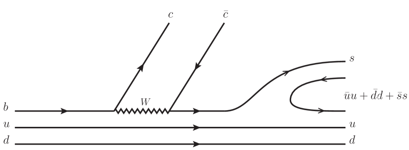
$\hskip 21.68231pt\underbrace{\hskip 216.81pt}_{\text{Weak decay}}\underbrace{\hskip 151.76964pt}_{\text{Hadronization}}\hskip 43.36464pt$

Figure 48: Production of a $K^{-}p$ pair from the weak decay ${\Lambda_{b}\to\Lambda\,J/\psi}$ via a hadronization mechanism. The full and wiggly lines correspond to quarks and the $W$-boson, respectively.

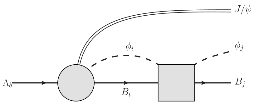
Figure 49: Final-state interaction of the meson-baryon pair, where the double, full and dashed lines denote the $J/\psi$, the baryons and the pseudoscalar mesons, respectively. The circle and square denote the production mechanism of the $J/\psi B_{i}\phi_{i}$ as depicted in Fig. 49 as well as meson-baryon scattering matrix $t_{ij}$, respectively

In this section we describe the reaction mechanism for the process[270] $\Lambda_{b}\to J/\psi\,\Lambda(1405)$, which is divided into three parts. The first two parts describe the decay mechanism $\Lambda_{b}\to J/\psi\,B\phi$, with $B\phi$ the meson-baryon system of strangeness $S=-1$, in the language of the quark model. Then, after hadronization, the final-state interaction is described in terms of the effective (hadronic) degrees of freedom of chiral perturbation theory (ChPT). After a resummation of the chiral meson-baryon potential to an infinite order, the $\Lambda(1405)$ is generated dynamically. In the following, we describe each single step of this reaction mechanism in more detail.

Weak decay: The $b$ quark of the $\Lambda_{b}$ undergoes the weak transition to a $c\bar{c}$ pair and an $s$-quark as depicted in the left part of Fig. 49. This transition is quantified by the matrix elements of the CKM matrix $V_{cb}V_{cs}^{*}$ and it is favored compared to $b\to c\bar{c}d$ leading to the $\Lambda_{b}\to J/\psi p\pi^{-}$, which was observed for the first time by the LHCb collaboration, see Ref. Aaij:2014zoa.

Hadronization: The $c\bar{c}$ pair forms the well-known $J/\psi$, while the virtual $uds$ three quark state undergoes hadronization to form a meson-baryon pair. This happens due to the large phase space available ($\leq 2522$ MeV for $M_{\Lambda_{b}}=5619$ MeV, $M_{J/\psi}=3097$ MeV), so that a quark-antiquark pair can become real, forming together with the three available quarks a meson-baryon pair. In principle, different meson-baryon states can be produced in such a mechanism. To determine their relative significance, we assume first that the $u$ and $d$ quarks of the original $\Lambda_{b}$ state are moving independently in a potential well. Further, we note that the $\Lambda_{b}$ ($J^{p}=1/2^{+}$) is in the ground state of the three-quarks $(udb)$. Therefore, all relative angular momenta between different quarks are zero. After the weak transition, but before the hadronization, the three-quark state $(uds)$ has to be in a p-wave since the final $\Lambda(1405)$ is a negative-parity state. On the other hand, since the $u$ and $d$ quarks are considered to be spectators and they were originally in $L=0$, the only possibility is that the $s$ quark carries the angular momentum, $L=1$. Moreover, since the final mesons and baryons are in the ground state and in s-wave to each other, all the angular momenta in the final state are zero. Consequently, the $\bar{q}q$ pair cannot be produced elsewhere, but between the $s$ quark and the $ud$ pair as depicted in Fig. 49. There are other possibilities to hadronize in which one of the original $u,d$ quarks goes into a meson and the $s$ quark into a baryon, followed by rescattering. However, these mechanisms are discussed in the next section and are suppressed due to large momentum transfers to the $u$ or $d$ quarks.

The flavour state of the initial $\Lambda_{b}$ can be written as

$$|\Lambda_{b}\rangle=\frac{1}{\sqrt{2}}|b(ud-du)\rangle\,,$$

turning after the weak process into

$$\frac{1}{\sqrt{2}}|s(ud-du)\rangle\,,$$

since the $u$ and $d$ quarks are considered to be spectators. Thus, after hadronization, the final quark flavor state is

$$|H\rangle \equiv\frac{1}{\sqrt{2}}|s\,(\bar{u}u+\bar{d}d+\bar{s}s)\,(ud-du)\rangle=\frac{1}{\sqrt{2}}\sum_{i=1}^{3}{|P_{3i}q_{i}(ud-du)}\rangle\,,$$

where we have defined

$$q\equiv\left(\begin{array}[]{c}u\\ d\\ s\end{array}\right)~{},$$

and $P$ denotes here the $M$ matrix defined in Eq. (13). We recall that it is in correspondence with the pseudoscalar meson matrix $\phi$ defined in Eq. (15). The hadronized state $|H\rangle$ can now be written as

$$|H\rangle=\frac{1}{\sqrt{2}}\bigg{(}K^{-}u(ud -du)+\bar{K}^{0}d(ud-du)+\frac{1}{\sqrt{3}}\left(-\eta+\sqrt{2}\eta^{\prime}\right)s(ud-du)\bigg{)}.$$

We can see that these states have overlap with the mixed antisymmetric baryon octet states [272]: octet baryons can be written as

$$|p\rangle= \frac{1}{\sqrt{2}}|u(ud-du)\rangle\,,$$

$$|n\rangle= \frac{1}{\sqrt{2}}|d(ud-du)\rangle\,,$$

$$|\Lambda\rangle= \frac{1}{\sqrt{12}}|(usd-dsu)+(dus-uds)+2(sud-sdu)\rangle\,.$$

Consequently, the hadronized state can be expressed in terms of the ground state meson and baryon octets as

$$|H\rangle=|K^{-}p\rangle+|\bar{K}^{0}n\rangle-\frac{\sqrt{2}}{3}|\eta\Lambda\rangle+\frac{2}{3}|\eta^{\prime}\Lambda\rangle\,,$$ (181)

which provides the relative weights between the final meson-baryon channels. Note that there is not direct production of $\pi\Sigma$ and $K\Xi$, however, these channels are present through the intermediate loops in the final state interaction as described below. Moreover, the final $\eta^{\prime}\Lambda$ channel will be neglected since it has a small effect due to its high mass and can be effectively reabsorbed in the regularization parameters as will be explained below.

Formation of the $\Lambda(1405)$: After the production of a meson-baryon pair, the final-state interaction takes place, which is parametrized by the scattering matrix $t_{ij}$. Thus, after absorbing the CKM matrix elements and kinematic prefactors into an overall factor $V_{p}$, the amplitude $\mathcal{M}_{j}$ for the transition $\Lambda_{b}\to J/\psi\,\phi_{j}B_{j}$ can be written as

$$\mathcal{M}_{j}(M_{\rm inv})=V_{p}\left(h_{j}+\sum_{i}h_{i}G_{i}(M_{\rm inv})\,t_{ij}(M_{\rm inv})\right)\,,$$ (182)

where, considering Eq. (181),

$$h_{\pi^{0}\Sigma^{0}}=h_{\pi^{+}\Sigma^{-}}=h_{\pi^{-}\Sigma^{+}}=0\,,~{}h_{\eta\Lambda}=-\frac{\sqrt{2}}{3}~{},$$

$$h_{K^{-}p}=h_{\bar{K}^{0}n}=1\,,~{}h_{K^{+}\Xi^{-}}=h_{K^{0}\Xi^{0}}=0~{},$$ (183)

and $G_{i}$ denotes the one-meson-one-baryon loop function, chosen in accordance with the models for the scattering matrix $t_{ij}$. Further, $M_{\rm inv}$ is the invariant mass of the meson-baryon system in the final state. Note also that the above amplitude holds for an $s$-wave only and every intermediate particle is put on the corresponding mass shell. Finally, the invariant mass distribution $\Lambda_{b}\to J/\psi\,\phi_{j}B_{j}$ reads

$$\frac{d\Gamma_{j}}{dM_{\rm inv}}(M_{\rm inv})=\frac{1}{(2\pi)^{3}}\frac{m_{j}}{M_{\Lambda_{b}}}{\rm\textbf{p}}_{J/\psi}{\rm\textbf{p}}_{j}\left|\mathcal{M}_{j}(M_{\rm inv})\right|^{2}\,,$$ (184)

where $\rm\textbf{p}_{J/\psi}$ and $\rm\textbf{p}_{j}$ denote the modulus of the three-momentum of the $J/\psi$ in the $\Lambda_{b}$ rest-frame and the modulus of the center-of-mass three-momentum in the final meson-baryon system, respectively. The mass of the final baryon is denoted by $m_{j}$.

As already described in the introduction, the baryonic $J^{P}=1/2^{-}$ resonance $\Lambda(1405)$ has to be understood as a dynamically generated state from the coupled-channel effects. The modern approach for it is referred to as chiral unitary models[250, 251, 11, 12, 252, 253, 15, 17, 254, 14, 18, 20, 21, 16, 273]. In the present approach we use the scattering amplitude from two very recent versions of such approaches, one from Ref. Mai:2014xna, that we call Bonn model and the other from Refs. Roca:2013av,Roca:2013cca, which we call MV model. While the basic motivation is the same for both approaches there are some differences, such as the order of truncation the underlying chiral potential as described in Ref. Roca:2015tea.

13.3 Results

After having set up the framework, we present here the predictions for the $\pi\Sigma$ and $\bar{K}N$ invariant mass distributions from the $\Lambda_{b}$ decay.

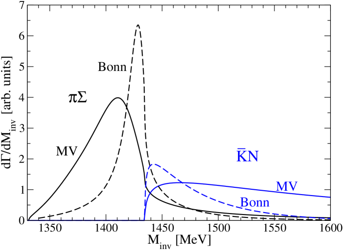
Figure 50: Results for the $\pi\Sigma$ and $\bar{K}N$ invariant mass distributions for the $\Lambda_{b}\to J/\psi\,\pi\Sigma$ and $\Lambda_{b}\to J/\psi\,\bar{K}N$ decays, respectively, for both models considered in the present work.

In Fig. 50 we show the final results for both the Bonn and MV models. In the $\pi\Sigma$ final state channel the peak of the $\Lambda(1405)$ is clearly visible. In fact, this is mostly due to the higher mass pole of the $\Lambda(1405)$ since the contribution proportional to $t_{\bar{K}N,\pi\Sigma}$ of Eq. (182) is the dominant one. The difference in the $\pi\Sigma$ mass distribution between both models is reminiscent of the fact that the Bonn model gets a narrower ($24\text{ MeV}$) highest $\Lambda(1405)$ pole than the MV model ($58\text{ MeV}$).

In the $\bar{K}N$ final state, the dominant contribution comes from the part proportional to $t_{\bar{K}N,\bar{K}N}$ which again is more sensitive to the higher mass $\Lambda(1405)$ pole. However, in this channel only the effect of the tail of the resonance is visible since the threshold of the $\bar{K}N$ mass distribution is located above the position of the $\Lambda(1405)$ peak. Nevertheless, that tail is enough to provide a high strength close to the threshold, what makes the line shape of the $\bar{K}N$ invariant mass distribution to be very different from just a phase-space distribution. The dependence on the choice of the model in this channel is due to the fact that the highest pole is slightly closer to threshold in the Bonn model compared to the MV one. Because of this feature, the Bonn model produces a narrower bump close to $\bar{K}N$ invariant mass threshold than the MV one. This observable is then very sensitive to the exact position of the resonance pole, due to the proximity between the threshold and the pole. As mentioned in the introduction, different reactions can reflect different weights for both poles of the $\Lambda(1405)$ resonance, depending on the particular production dynamics. In the present case, the highest pole is the one that shows up dominantly.

On the other hand, the agreement in Fig. 50 of the results between the MV and Bonn models is remarkable, given their theoretical differences and fitting strategies used in them. Nonetheless we can regard the difference between the models as the main source of the theoretical uncertainty.

While the overall normalization of the invariant mass distributions is unknown, the shape and the ratio between the $\pi\Sigma$ and $\bar{K}N$ distributions is unchanged and it is a genuine prediction. Indeed, the ratio between the maximum values of the $\pi\Sigma$ and $\bar{K}N$ distribution is 3.3 for the MV and 3.5 for the Bonn model. The value of that ratio as well as the shape of the distributions are then genuine predictions of the chiral unitary approach. In conclusion, Fig. 50 serves to predict the invariant mass distributions of either $\pi\Sigma$ or $\bar{K}N$, once the absolute normalization of the mass distribution of the other channel has been measured. For instance, if the LHCb[271] and CDF[276] collaboration were to measure the $K^{-}p$ mass distribution in the $\Lambda_{b}\to J/\psi~{}K^{-}p$ decay, then the shape should agree with the prediction of Fig. 50 and once normalized, the $\bar{K}N$ and $\pi\Sigma$ distributions would be given both in size and shape.

14 The $\Lambda_{b}\to J/\psi~{}K~{}\Xi$ decay and the higher order chiral terms of the meson baryon interaction.

This work is complementary to the one shown in the former subsection.

14.1 Formalism

14.1.1 The $\Lambda_{b}\to J/\psi~{}M~{}B$ process

At the quark level, the Cabibbo favored mechanism for $J/\psi$ production in $\Lambda_{b}$ decay is depicted by the first part of the diagram of Fig. 49. This corresponds to internal emission in the classification of topologies of Ref. Chau:1982da, and is also the dominant mechanism in the related $\bar{B}^{0}\to J/\psi~{}\pi~{}\pi$ decay[48]. As we can see in the figure, a $sud$ state is obtained after the weak decay. The next step consists in the hadronization of this final three quark state by introducing a $\bar{q}q$ pair with the quantum numbers of the vacuum, $\bar{u}u+\bar{d}d+\bar{s}s$, which will then produce an initial meson-baryon pair. As in the former section, in this reaction the $u$ and $d$ quarks act as spectators. This means that the $ud$ pair in the final $sud$ state after the weak decay has $I=0$ and, since the $s$ quark also has $I=0$, the final three-quark system has total $I=0$. Hence, even if the weak interaction allows for isospin violation, in this case the process has filtered $I=0$ in the final state. Since isospin is conserved in the strong hadronization process and in the subsequent final state rescattering interaction, the final meson-baryon component also appears in $I=0$.

As already discussed in Sec. 13, another observation concerning the hadronization is that, since the $sud$ quark state after the weak decay has $J^{P}=1/2^{-}$ and the $ud$ quarks have the same quantum numbers as in the original $\Lambda_{b}$ state ($J^{P}=1/2^{+}$ each) in an independent quark model used for the argumentation, it is the $s$ quark the one that must carry the minus parity, which would correspond to an $L=1$ orbit of a potential well. Since the final meson-baryon states are all in their ground state, the $s$ quark must de-excite and hence it must participate in the hadronization. This latter process gives rise to some meson-bayon states with the weight given earlier in Eqs. (183). As usual in these studies, we neglect the $\eta^{\prime}\Lambda$ component, and we only have primary $K^{-}p$, $K^{0}n$ or $\eta\Lambda$ production. We can see that a $K\Xi$ pair is not produced in the first step.

Next, one must incorporate the final state interaction of these meson-baryon pairs, which is depicted in Fig. 49. The matrix element for the production of the final state, $j$, is given by Eq. (182). The factor $V_{p}$, which includes the common dynamics of the production of the different pairs, is unknown and we take it as constant. Finally, the invariant mass distribution $\Lambda_{b}\to J/\psi\,\phi_{j}\,B_{j}$ is given by Eq. (184).

14.2 Results

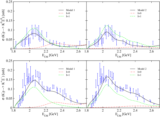
Figure 51: (Color online) The total cross sections of the $K^{-}p\to K^{0}\Xi^{0}$ reaction (top row) and the $K^{-}p\to K^{-}\Xi^{+}$ reaction (bottom row) for the two different models (Model 1 and Model 2) discussed in the text. The solid lines show the results of the full amplitude, while the dashed and dash-dotted lines denote the $I=1$ and $I=0$ contributions, respectively. Theoretical values are compared with experimental data[277, 278, 279, 280, 281, 282, 283].

We start this section by presenting in Fig. 51 the cross section data of the $K^{-}p\to K^{0}\Xi^{0}$ reaction (top panels) and of the $K^{-}p\to K^{-}\Xi^{+}$ reaction (bottom panels), obtained employing Model 1 (left panels) or Model 2 (right panels) [284]. The figure shows the complete results (solid lines), as well as the results where only the isospin $I=1$ component (dashed lines) or the $I=0$ one (dash-dotted lines) have been retained. It is interesting to see that, in both models, the $I=1$ component is dominant and is concentrated at lower energies. The smaller $I=0$ component at higher energies adds up destructively to the cross section in the case of the $K^{-}p\to K^{0}\Xi^{0}$ reaction, while it contributes to enhance the cross section in the $K^{-}p\to K^{-}\Xi^{+}$ process. We note that the tree-level chiral contributions to these reactions come entirely from the NLO Lagrangian and, upon inspecting the size of the coefficients, their strength in the $I=0$ channel would be nine times larger than that in the $I=1$ channel. The reversed trend observed in Fig. 51 is a consequence of the unitarization in coupled channels with coupling coefficients determined by the fit and, consequently, by the data.

As we can see in Fig. 51, the contribution of $I=0$ in the $K^{-}p\to K\Xi$ cross section has a maximum around 2300 MeV for Model 1 or around 2400 MeV and less pronounced for Model 2, far from the peak of the data and of the complete amplitude, around 2050 MeV. The $K^{-}p\to K\Xi$ reactions contain a mixture of both isospin components, while the decay process $\Lambda_{b}\to J/\psi~{}K~{}\Xi$, studied in this paper, filters $I=0$ and therefore provides additional information to the one obtained from the scattering data.

Figure 52: Invariant mass distributions of $\pi\Sigma$ and $\bar{K}N$ states in the decay modes $\Lambda_{b}\to J/\psi~{}\pi~{}\Sigma$ and $\Lambda_{b}\to J/\psi~{}\bar{K}~{}N$, for the two models discussed in the text: Model 1 (dashed lines) and Model 2 (solid lines). The units in the $y$ axis are obtained taking $V_{p}=1$.

Since the models of Ref. Feijoo:2015yja make a fitting to all $K^{-}p\to X$ data in a range from threshold to $K\Xi$ production, we start presenting, in Fig. 52, what are the predictions of Model 1 and Model 2 for the decay reactions $\Lambda_{b}\to J/\psi~{}\bar{K}~{}N$ and $\Lambda_{b}\to J/\psi~{}\pi~{}\Sigma$, already studied in the former section. These are averaged distributions over the possible different charged states. We can see that the results of both models are similar to those found in Sec. 13, with the shape of the $\pi\Sigma$ and $\bar{K}N$ distributions lying somewhat in between those of the Bonn and Murcia-Valencia models studied there (a different normalization is used in that work). We note that our $\pi\Sigma$ distributions shown in Fig. 52 stay over the ${\bar{K}}N$ ones, in contrast to what one observes in Fig. 50, where the $\pi\Sigma$ distributions cross below the respective ${\bar{K}}N$ ones just above the threshold for ${\bar{K}}N$ states. This is a peculiarity of the NLO contributions, since one also obtains a crossing behavior when the interaction models are restricted to only the lowest order terms. It is also interesting to see that the numerical results in Fig. 52 depend on the model, indicating their sensitivity on different parametrizations that fit equally well the $K^{-}p\to X$ data. We obtain ratios of 4.9 and 3.5 for Models 1 and 2, respectively. These values are of the order of those found in the former section.

In Fig. 53 we present the invariant mass distributions of the $K^{+}\Xi^{-}$ states from the decay process $\Lambda_{b}\to J/\psi~{}K^{+}~{}\Xi^{-}$. We do not show the distribution for the decay process $\Lambda_{b}\to J/\psi~{}K^{0}~{}\Xi^{0}$, because, except for minor differences associated to the slightly different physical masses of the particles, it is identical to that of the charged channel, since these processes involve only the $I=0$ part of the strong meson-baryon amplitude. The fact that this decay filters the $I=0$ components makes the differences between Model 1 (thick dashed line) and Model 2 (thick solid line) to be more evident, not only in the strength but also in the shape of the invariant mass distribution. If, in order to eliminate the dependence on undetermined loop functions and on the unknown weak parameter $V_{p}$, we represented each $\Lambda_{b}\to J/\psi~{}K^{+}~{}\Xi^{-}$ distribution relative to its corresponding $\Lambda_{b}\to J/\psi~{}{\bar{K}}~{}N$ one shown in Fig. 52, the difference would even be somewhat enhanced. Therefore, measuring the decay of the $\Lambda_{b}$ into $J/\psi~{}K^{+}~{}\Xi^{-}$ and into J$/\psi~{}{\bar{K}}~{}N$ could help in discriminating between models that give a similar account of the scattering $K^{-}p\to K^{0}\Xi^{0},K^{+}\Xi^{-}$ processes. The figure also shows that the $I=0$ structure observed around 2300 MeV results from the terms of the NLO Lagrangian. When they are set to zero, the invariant mass distributions of the two models, shown by the thin dashed and thin solid lines in Fig. 53, become small and structureless.

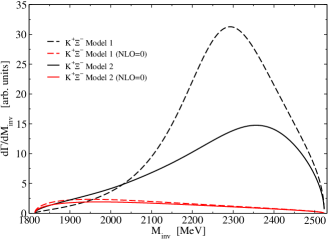
Figure 53: (Color online) Invariant mass distributions of $K^{+}\Xi^{-}$ states produced in the decay $\Lambda_{b}\to J/\psi~{}K^{+}~{}\Xi^{-}$, obtained for the two models discussed in the text: Model 1 (dashed lines) and Model 2 (solid lines). The thin lower lines correspond to omitting the NLO terms of the potential. The normalization is the same as in Fig. 52.

We have observed a similar behaviour in the mass distributions of the reaction $\Lambda_{b}\to J/\psi~{}\eta~{}\Lambda$ which are shown in Fig. 54. In this case, as the coefficient $h_{\eta\Lambda}$ does not vanish, we see from Eq. (182) that the tree level term also contributes here, unlike the case of $K\Xi$ production. This makes the magnitude of the $\Lambda_{b}\to J/\psi~{}\eta~{}\Lambda$ mass distribution about twenty times bigger than that of the $\Lambda_{b}\to J/\psi~{}K~{}\Xi$ one.

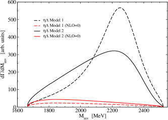
Figure 54: (Color online) Invariant mass distributions of $\eta\Lambda$ states produced in the decay $\Lambda_{b}\to J/\psi~{}\eta~{}\Lambda$, obtained for the two models discussed in the text: Model 1 (dashed lines) and Model 2 (solid lines). The thin lower lines correspond to omitting the NLO terms of the potential. The normalization is the same as in Fig. 52.

The invariant mass distributions from the $\Lambda_{b}\to J/\psi~{}K^{+}~{}\Xi^{-}$ and $\Lambda_{b}\to J/\psi~{}\eta~{}\Lambda$ decays obtained in Models 1 and 2 are compared with phase space in Fig. 55. The phase-space distributions (dotted lines for Model 1 and dash-dotted lines for Model 2) are obtained by taking the amplitude $\mathcal{M}_{j}$ as constant in Eq. (184) and normalizing to the area of the invariant mass distribution of the corresponding model. The comparison allows one to see that there are dynamical features in the meson-baryon amplitudes leading to a distinct shape of the mass distributions. In the case of Model 1, we observe a peak between 2250 MeV and 2300 MeV for both $\Lambda_{b}\to J/\psi~{}K^{+}~{}\Xi^{-}$ and $\Lambda_{b}\to J/\psi~{}\eta~{}\Lambda$ distributions. The peak resembles a resonance, but we should take into account that the limitation of the phase space at about 2500 MeV produces a narrower structure than that of the cross sections of the $K^{-}p\to K\Xi$ reactions, as we can see from the $I=0$ contribution in Fig. 51 (left panels), which is much broader. Actually, the $I=0$ contribution of Model 2 to the cross sections of Fig. 51 (right panels) does not indicate any particular structure, and the very different shapes that this model predicts for $\Lambda_{b}\to J/\psi~{}K^{+}~{}\Xi^{-}$ and $\Lambda_{b}\to J/\psi~{}\eta~{}\Lambda$ (see the thick solid lines in Fig. 55), peaking at about 2400 MeV and 2200 MeV respectively, do not indicate the presence of a resonance since it would necessarily appear in both final states at the same energy. In our models, it is the energy dependence in the parametrization of the next-to-leading order contribution and the interference of terms what creates this shape. In any case, what is clear is that the experimental implementation of this reaction will provide valuable information concerning the meson-baryon interaction at higher energies, beyond what present data of scattering has offered us.

Although we have given the invariant mass distributions in arbitrary units, one should bear in mind that all the figures, from Fig. 52 to Fig. 54 have the same normalization. Since measurements for the $\Lambda_{b}\to J/\psi~{}K^{-}~{}p$ reaction are already available from the CDF[285] and LHCb[286, 271, 287] collaborations, the measurements of the reactions proposed here could be referred to those of the $\Lambda_{b}\to J/\psi~{}K^{-}~{}p$ reaction and this would allow a direct comparison with our predictions. In this spirit, we note that the recent resonance analysis of Ref. Aaij:2015tga shows a $\Lambda(1405)$ contribution which lies in between the distribution found by the Bonn model in Ref. Roca:2015tea and that of the Murcia-Valencia model in Ref. Roca:2015tea or the Barcelona models presented here. Further details and discussions on the reaction and the results can be seen in Ref. Feijoo:2015cca.

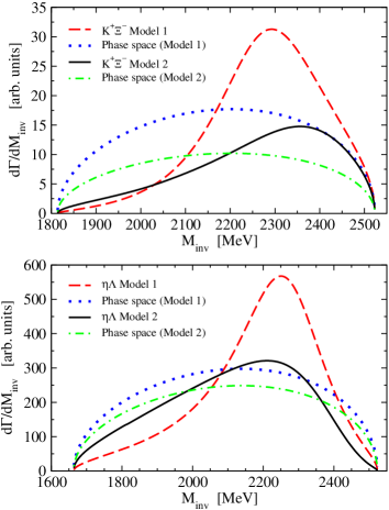
Figure 55: (Color online) Comparison of the invariant mass distributions of $K^{+}\Xi^{-}$ states (upper panel) and $\eta\Lambda$ states (lower panel) states obtained with Model 1 (dashed lines) and Model 2 (solid lines) with a pure phase-space distribution (dotted lines)

15 Weak decay of $\Lambda_{c}^{+}$ for the study of $\Lambda(1405)$ and $\Lambda(1670)$

15.1 Formulation

We consider the decay process $\Lambda_{c}^{+}\to\pi^{+}\Lambda^{*}\to\pi^{+}MB$, where $MB$ stands for the final meson-baryon states such as $\pi\Sigma$ and $\bar{K}N$. We show that, when the $MB$ invariant mass is restricted in the $\Lambda(1405)$ region, the dominant contribution of this decay process is given by the diagram shown in Fig. 56.

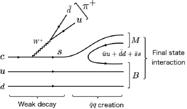
Figure 56: The dominant diagram for the $\Lambda_{c}^{+}\to\pi^{+}MB$ decay. The solid lines and the wiggly line show the quarks and the $W$-boson, respectively.

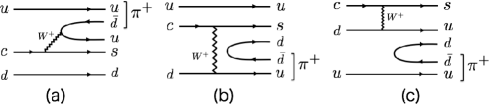
Figure 57: The dominant diagram for the $\Lambda_{c}^{+}\to\pi^{+}MB$ decay. The solid lines and the wiggly line show the quarks and the $W$-boson, respectively.

First, the charm quark in $\Lambda_{c}^{+}$ turns into the strange quark with the $\pi^{+}$ emission by the weak decay. Second, the $\bar{q}q$ creation occurs to form $M$ ($B$) from the $s$ quark ($ud$ diquark). Finally, considering the final state interactions of the hadrons, we obtain the invariant mass distribution for the $\Lambda_{c}^{+}\to\pi^{+}MB$ process. In the following, we will discuss these three steps separately.

15.1.1 Weak decay

We first discuss the decay of $\Lambda_{c}$ to produce $\pi^{+}$ and the $sud$ cluster in the final state. The Cabibbo favored weak processes are given by

$$c\to s+u+\bar{d}\quad\text{: $c$ decay},$$ (185)

$$c+d\to s+u\quad\text{: $cd$ scattering}.$$ (186)

The diagram shown in Fig. 56 is obtained by the $c$ decay process. Another contribution with the $c$ decay is to form $\pi^{+}$ using the $u$ quark in $\Lambda_{c}$ [Fig. 57(a)]. In this process, however, the color of the $u\bar{d}$ pair from the $W^{+}$ decay is constrained to form the color singlet $\pi^{+}$. This process is therefore suppressed by the color factor in comparison with Fig. 56. In addition, because the $ud$ diquark in $\Lambda_{c}$ is the most attractive “good” diquark [289], the process to destruct the strong diquark correlation [Fig. 57(a)] is not favored. The contribution from the $cd$ scattering Eq. (186) [Fig. 57(b) and (c)] is suppressed by the additional creation of a $\bar{q}q$ pair not attached to the $W$-boson as well as the $1/N_{c}$ suppression, compared with Fig. 56. Diagrams  57(b) and  57(c) are called “absorption diagrams” in the classification of Ref. Chau:1982da, and they are two body processes, involving two quarks of the original $\Lambda_{c}$, which are suppressed compared to the one body process (Fig. 56) involving only the $c$ quark, the $u$, $d$ quarks acting as spectators. A discussion of this suppression is done in section 5.

As discussed in Ref. Hyodo:2011js, the kinematical condition also favors the diagram shown in Fig. 56. When the $\Lambda_{c}$ decays into $\pi^{+}$ and $MB$ system with the invariant mass of 1400 MeV, the three momentum of the final state is $\sim 700$ MeV in the rest frame of $\Lambda_{c}$. Thus, the $\pi^{+}$ should be emitted with a large momentum. It is kinematically favored to create the fast pion from the quarks involved by the weak process, because of the large mass of the $c$ quark. The diagrams Fig 57(a) and (c) are suppressed because one of the spectator quarks is required to participate in the $\pi^{+}$ formation.

In this way, the diagram in Fig. 56 is favored from the viewpoint of the CKM matrix, color suppression, the diquark correlation, and the kinematical condition. We note that this diagram has a bigger strength than the dominant one of the $\Lambda_{b}\to J/\psi\Lambda(1405)$ decay discussed in the two former sections, in which the weak process contains the necessary Cabibbo suppressed $b\to c$ transition and proceeds via internal emission[111] where the color of every quark in the weak process is fixed.

In this process, because the $ud$ diquark in $\Lambda_{c}$ is the spectator, the $sud$ cluster in the final state is combined as

$$\frac{1}{\sqrt{2}}|s(ud-du)\rangle.$$

This combination is a pure $I=0$ state. Because the $\bar{q}q$ creation does not change the isospin, we conclude that the dominant contribution for the $\Lambda_{c}\to\pi^{+}MB$ process produces the $MB$ pair in $I=0$. We note that the unfavored diagrams that we neglect can produce the $sud$ state with $I=1$. We will revisit the $I=1$ contribution at the end of Sec. 15.2.

15.1.2 $\bar{q}q$ creation

To create the $MB$ final state, we must proceed to hadronize the $sud$ state, creating an extra $\bar{q}q$ pair, as we have done in the former sections. Since the total spin-parity of the $MB$ pair is $J^{P}=1/2^{-}$, the $s$ quark should be in $L=1$ after the $c$ quark decay, together with the spectator $ud$ diquark. To achieve the final $MB$ state where all quarks are in the ground state, the $\bar{q}q$ creation must involve the $s$ quark to deexcite into $L=0$. Then the hadronization proceeds as depicted in Fig. 56, where the $s$ quark goes into the meson $M$ and the $ud$ diquark is used to form the baryon $B$. Another possibility, the formation of the baryon from the $s$ quark, is not favored because of the correlation of the good $ud$ diquark and the suppression discussed above by forcing a spectator quark from the $\Lambda_{c}$ to form the emerging meson. Other possibilities of hadronization are also discussed in Ref. Miyahara:2015cja, concluding that they are suppressed.

To evaluate the relative fractions of the $MB$ state, we follow the same procedure with Ref. Roca:2015tea. Using these hadronic representations, we obtain the meson-baryon states after the $\bar{q}q$ pair production as

$$|MB\rangle =|K^{-}p\rangle+|\bar{K}^{0}n\rangle-\frac{\sqrt{2}}{3}|\eta\Lambda\rangle.$$ (187)

Here we neglect the irrelevant $\eta^{\prime}\Lambda$ channel because its threshold is above 2 GeV. We can see that we obtain the isospin $I=0$ $\bar{K}N$ combination in the phase convention that we use where $|K^{-}\rangle=-|I=1/2,I_{z}=-1/2\rangle$.

15.1.3 Final state interaction

Here we derive the decay amplitude $\mathcal{M}$, taking the final state interaction of the $MB$ pair into account. As shown in Fig. 58, the final state interaction consists of the tree part and the rescattering part.

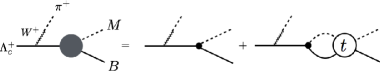
Figure 58: The diagram for the meson-baryon final state interaction (filled circle) as the sum of the tree part (dot) and the rescattering part with the meson-baryon scattering amplitude (unfilled circle).

The rescattering of the $MB$ pair is described by the chiral unitary approach [250, 11, 12, 252, 292], which is based on the chiral Lagrangians and is constructed to treat the non-perturbative phenomena. Though only the $K^{-}p,\ \bar{K^{0}}n,\ \eta\Lambda$ states appear in Eq. (187) in the tree-level production, the coupled-channel scattering leads to the other $MB$ states, $\pi^{0}\Sigma^{0}$, $\pi^{-}\Sigma^{+}$, $\pi^{+}\Sigma^{-}$, $\pi^{0}\Lambda$, $K^{-}p$, $\bar{K^{0}}n$, $\eta\Lambda$, $\eta\Sigma^{0}$, $K^{+}\Xi^{-}$, $K^{0}\Xi^{0}$. The decay amplitude for the $\Lambda_{c}\to\pi^{+}(MB)_{j}$ with the meson-baryon channel $j$ can then be written as Eq. (182), with the same weights for $h_{i}$. The weak decay and the $\bar{q}q$ pair creation are represented by the factor $V_{P}$ in Eq. (182), which is assumed to be independent of the invariant mass $M_{\rm inv}$ in the limited range of invariant masses that we consider. Explicit forms for the $t$-matrices of Eq. (182) can be found in different works[250, 11, 12, 252, 292]. It is also instructive for practical calculations to show the amplitude in the isospin basis. If we assume the isospin symmetry, the amplitude of the decay to the $\pi\Sigma$ and $\bar{K}N$ channels are written as

$$\mathcal{M}_{\pi^{0}\Sigma^{0}} =\mathcal{M}_{\pi^{-}\Sigma^{+}}=\mathcal{M}_{\pi^{+}\Sigma^{-}}=V_{P}\left(-\sqrt{\frac{2}{3}}G_{\bar{K}N}t^{I=0}_{\bar{K}N,\pi\Sigma}+\frac{\sqrt{2}}{3\sqrt{3}}G_{\eta\Lambda}t^{I=0}_{\eta\Lambda,\pi\Sigma}\right),$$ (188)

$$\mathcal{M}_{K^{-}p} =\mathcal{M}_{\bar{K^{0}}n}=V_{P}\left(1+G_{\bar{K}N}t^{I=0}_{\bar{K}N,\bar{K}N}-\frac{1}{3}G_{\eta\Lambda}t^{I=0}_{\eta\Lambda,\bar{K}N}\right).$$ (189)

The partial decay width of the $\Lambda_{c}$ into the $\pi^{+}(MB)_{j}$ channel is given by

$$\Gamma_{j} =\int d\Pi_{3}|\mathcal{M}_{j}|^{2},$$ (190)

where $d\Pi_{3}$ is the three-body phase space. The invariant mass distribution is obtained as the derivative of the partial width with respect to $M_{\rm inv}$. In the present case, because the amplitude $\mathcal{M}_{j}$ depends only on $M_{\rm inv}$, the mass distribution ${\rm d}\Gamma_{j}/{\rm d}M_{\rm inv}$ is obtained by integrating the phase space as

$$\frac{{\rm d}\Gamma_{j}}{{\rm d}M_{\rm inv}} =\frac{1}{(2\pi)^{3}}\frac{p_{\pi^{+}}\tilde{p}_{j}M_{\Lambda_{c}^{+}}M_{j}}{M_{\Lambda_{c}^{+}}^{2}}|\mathcal{M}_{j}|^{2},$$ (191)

where $M_{j}$ is the baryon mass, and $p_{\pi^{+}}$ and $\tilde{p}_{j}$ represent the magnitude of the three momentum of the emitted $\pi^{+}$ by the weak decay in the $\Lambda_{c}$ rest frame and of the meson of the final meson-baryon state in the meson-baryon rest frame, respectively.

Since the $\Lambda(1405)$ is mainly coupled to the $\pi\Sigma$ and $\bar{K}N$ channels, we calculate the invariant mass distribution of the decay to the $\pi\Sigma$ and $\bar{K}N$ channels. For the study of the $\Lambda(1670)$, we also calculate the decay to the $\eta\Lambda$ channel.

15.2 Results

We present the numerical results of the $MB$ invariant mass spectra in the $\Lambda_{c}\to\pi^{+}MB$ decay. We first show the results in the energy region near the $\bar{K}N$ threshold where the $\Lambda(1405)$ resonance plays an important role. We then discuss the spectra in the higher energy region with the emphasis of the $\Lambda(1670)$ resonance. The decay branching fractions of $\Lambda_{c}$ into different final states are discussed at the end of this section.

15.2.1 Spectrum near the $\bar{K}N$ threshold

To calculate the region near the $\bar{K}N$ threshold quantitatively, the final state interaction of the $MB$ system should be constrained by the new experimental data from the SIDDHARTA collaboration [293, 294], because the precise measurement of the energy-level shift of kaonic hydrogen significantly reduces the uncertainty of the scattering amplitude below the $\bar{K}N$ threshold. Here we employ the meson-baryon amplitude in Refs. Ikeda:2012au,Ikeda:2011pi, which implements the next-to-leading order terms in chiral perturbation theory to reproduce the low-energy $\bar{K}N$ scattering data, including the SIDDHARTA constraint. The isospin symmetry breaking is introduced by the physical values for the hadron masses. In this model, the two resonance poles of the $\Lambda(1405)$ are obtained at $1424-26i$ MeV and $1381-81i$ MeV.

We show the spectra of three $\pi\Sigma$ channels in Fig. 59. From this figure, we find the $\Lambda(1405)$ peak structure around 1420 MeV. It is considered that the peak mainly reflects the pole at $1424-26i$ MeV. Because the initial state contains the $\bar{K}N$ channel with vanishing $\pi\Sigma$ component as shown in Eq. (187), the present reaction puts more weight on the higher energy pole which has the strong coupling to the $\bar{K}N$ channel.

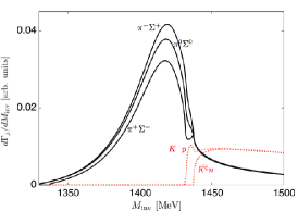
Figure 59: (Color online) Invariant mass distribution of the decay $\Lambda_{c}^{+}\to\pi^{+}MB$ near the $\bar{K}N$ threshold. The solid line represents the spectrum for $\pi\Sigma$ channels and the dashed line for $\bar{K}N$ channels. The meson-baryon amplitude is taken from the work of Ikeda et al.[16].

To proceed further, let us recall the isospin decomposition of the $\pi\Sigma$ channels [296]. The particle basis and the isospin basis are related as follows,

$$|\pi^{0}\Sigma^{0}\rangle =-\frac{1}{\sqrt{3}}|\pi\Sigma\rangle^{I=0}-\sqrt{\frac{2}{3}}|\pi\Sigma\rangle^{I=2},$$

$$|\pi^{-}\Sigma^{+}\rangle =-\frac{1}{\sqrt{3}}|\pi\Sigma\rangle^{I=0}-\frac{1}{\sqrt{2}}|\pi\Sigma\rangle^{I=1}-\frac{1}{\sqrt{6}}|\pi\Sigma\rangle^{I=2},$$ (192)

$$|\pi^{+}\Sigma^{-}\rangle =-\frac{1}{\sqrt{3}}|\pi\Sigma\rangle^{I=0}+\frac{1}{\sqrt{2}}|\pi\Sigma\rangle^{I=1}-\frac{1}{\sqrt{6}}|\pi\Sigma\rangle^{I=2}.$$

In general reactions, the initial state of the $MB$ amplitude is a mixture of the $I=0$ and $I=1$ components. The charged $\pi\Sigma$ spectra thus contain the $I=1$ contribution as well as the interference effects of different isospin components.

It is therefore remarkable that all the $\pi\Sigma$ channels have the same peak position in Fig. 59. This occurs because the present reaction picks up the $I=0$ initial state selectively, as explained in Sec. 15.1. In this case, the $I=1$ contamination is suppressed down to the isospin breaking correction, and hence all the charged states exhibit almost the same spectrum. The differences of the spectra, because of the $I=0$ filter in the present reaction, are much smaller than in photoproduction [261, 297], where the explicit contribution of the $I=0$ and $I=1$ channels makes the differences between the different $\pi\Sigma$ channels much larger, even changing the position of the peaks. In this respect, the $\Lambda_{c}\to\pi^{+}\pi\Sigma$ reaction is a useful process to extract information on the $\Lambda(1405)$, because even in the charged states (the $\pi^{0}\Sigma^{0}$ automatically projects over $I=0$) one filters the $I=0$ contribution and the charged states are easier to detect in actual experiments.

The spectra for the $\bar{K}N$ channels are also shown in Fig. 59. In the $\bar{K}N$ channels, the peak of the $\Lambda(1405)$ cannot be seen, because the $\bar{K}N$ threshold is above the $\Lambda(1405)$ energy. However, the enhancement near the threshold that we observe in Fig. 59 is related to the tail of the $\Lambda(1405)$ peak. The shape of the $\bar{K}N$ spectrum, as well as its ratio to the $\pi\Sigma$ one, is the prediction of the meson-baryon interaction model. The detailed analysis of the near-threshold behavior of the $\bar{K}N$ spectra, together with the $\pi\Sigma$ spectra, will be important to understand the nature of the $\Lambda(1405)$.

15.2.2 Spectrum above the $\bar{K}N$ threshold

The spectrum above the $\bar{K}N$ threshold is also interesting. The LHCb collaboration has found that a substantial amount of $\Lambda^{*}$s is produced in the $K^{-}p$ spectrum in the $\Lambda_{b}\to J/\psi K^{-}p$ decay [287]. Hence, the $K^{-}p$ spectrum in the weak decay process serves as a new opportunity to study the excited $\Lambda$ states.

For this purpose, here we adopt the model in Ref. Oset:2001cn for the meson-baryon final state interaction, which reproduces the $\Lambda(1670)$ as well as the $\Lambda(1405)$ in the $I(J^{P})=0(1/2^{-})$ channel. The pole position of the $\Lambda(1670)$ is obtained at $1678-20i$ MeV. Since the width of the $\Lambda(1670)$ is narrow, the pole of the $\Lambda(1670)$ also affects the invariant mass distribution of the $\Lambda_{c}^{+}$ decay.

In Fig. 60, we show the invariant mass distribution of the $\Lambda_{c}^{+}$ decay into the $\pi\Sigma$, $\bar{K}N$ and $\eta\Lambda$ channels. Because the meson-baryon amplitude in Ref. Oset:2001cn does not include the isospin breaking effect, all the isospin multiplets $\{K^{-}p,\bar{K}^{0}n\}$, $\{\pi^{0}\Sigma^{0},\pi^{+}\Sigma^{-},\pi^{-}\Sigma^{+}\}$ provide an identical spectrum. Because the $\Lambda(1520)$ resonance in $d$ wave is not included in the amplitude, such contribution should be subtracted to compare with the actual spectrum.

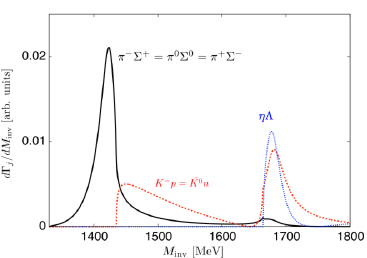
Figure 60: (Color online) Invariant mass distribution of the decay $\Lambda_{c}^{+}\to\pi^{+}MB$. The solid, dotted, and dash-dotted lines represent the $\bar{K}N=\{K^{-}p,\ \bar{K^{0}}n\}$, $\pi\Sigma=\{\pi^{0}\Sigma^{0},\ \pi^{-}\Sigma^{+},\ \pi^{+}\Sigma^{-}\}$, and $\eta\Lambda$ channels, respectively. The meson-baryon amplitude is taken from Oset et al.[253] where the $\Lambda(1520)$ contribution in $d$ wave is not included.

As in the previous subsection, we find the $\Lambda(1405)$ peak structure in the $\pi\Sigma$ channel and the threshold enhancement in the $\bar{K}N$ channel. Furthermore, in the higher energy region, we find the additional peak structure of the $\Lambda(1670)$ around 1700 MeV in all channels. Especially, the peak is clearly seen in the $\bar{K}N$ and $\eta\Lambda$ channels, as a consequence of the stronger coupling of the $\Lambda(1670)$ to these channels than to the $\pi\Sigma$ channel[253]. The $\eta\Lambda$ channel is selective to $I=0$, and the $\Lambda(1520)$ production is kinematically forbidden.

We expect that the structure of the $\Lambda(1670)$ can be analyzed from the measurements of the $\Lambda_{c}^{+}$ decay to the $\bar{K}N$ and $\eta\Lambda$ channels.

15.2.3 Branching fractions

Experimentally, the decay branching fractions of $\Lambda_{c}\to\pi^{+}MB$ are determined as[95]:

$$\Gamma(\Lambda_{c}\to pK^{-}\pi^{+},\text{nonresonant}) =2.8\pm 0.8\%$$ (193)

$$\Gamma(\Lambda_{c}\to\Sigma^{+}\pi^{+}\pi^{-}) =3.6\pm 1.0\%$$ (194)

$$\Gamma(\Lambda_{c}\to\Sigma^{-}\pi^{+}\pi^{+}) =1.7\pm 0.5\%$$ (195)

$$\Gamma(\Lambda_{c}\to\Sigma^{0}\pi^{+}\pi^{0}) =1.8\pm 0.8\%$$ (196)

where the nonresonant component is obtained by subtracting the contributions from the $K^{*}(892)^{0}$, $\Delta(1232)^{++}$, and $\Lambda(1520)$ in the $K^{-}\pi^{+}$, $p\pi^{+}$, and $pK^{-}$ spectra, respectively. Taking the ratios of the central values, we obtain

$$\frac{\Gamma(\Lambda_{c}\to\Sigma^{+}\pi^{+}\pi^{-})}{\Gamma(\Lambda_{c}\to pK^{-}\pi^{+},\text{nonresonant})} =1.29$$ (197)

$$\frac{\Gamma(\Lambda_{c}\to\Sigma^{-}\pi^{+}\pi^{+})}{\Gamma(\Lambda_{c}\to pK^{-}\pi^{+},\text{nonresonant})} =0.61$$ (198)

$$\frac{\Gamma(\Lambda_{c}\to\Sigma^{0}\pi^{+}\pi^{0})}{\Gamma(\Lambda_{c}\to pK^{-}\pi^{+},\text{nonresonant})} =0.64~{}.$$ (199)

In principle, these ratios can be calculated in the present model by integrating Eq. (191) over $M_{\rm inv}$. However, in the present calculation, we consider the process which is dominant in the small $M_{\rm inv}$ region, as explained in Sec. 15.1. At large $M_{\rm inv}$ region, processes other than those considered can contribute. Also, higher excited $\Lambda^{*}$ states and resonances in the $\pi^{+}M$ and $\pi^{+}B$ channels may play an important role, as shown in the former section. In this way, the validity of the present framework is not necessarily guaranteed for the large $M_{\rm inv}$ region.

Nevertheless, it is worth estimating the branching ratios by simply extrapolating the present model. The theoretical estimate of the ratio of the decay fraction is obtained as

$$\frac{\Gamma_{\pi^{-}\Sigma^{+}}}{\Gamma_{K^{-}p}}=\begin{cases}1.05&(\text{Ref.~{}\refcite{Ikeda:2012au}})\\ 0.95&(\text{Ref.~{}\refcite{Oset:2001cn}})\end{cases}.$$ (200)

Given the uncertainties in the experimental values and the caveats in the extrapolation discussed above, it is fair to say that the gross feature of the decay is captured by the present model. We note that the difference of the charged $\pi\Sigma$ states in our model is of the order of the isospin breaking correction. The large deviation in the experimental data, albeit nonnegligible uncertainties, may indicate the existence of mechanisms which are not included in the present framework. It is worth noting that in the theoretical model of Ref. Ikeda:2012au the $\pi^{-}\Sigma^{+}\pi^{+}$ channel has the largest strength as in the experiment.

Let us also mention the measured value of the branching fraction $\mathcal{B}(\Lambda_{c}\to\Lambda\pi^{+}\pi^{0})=3.6\pm 1.3\%$ [95]. Because $\pi^{0}\Lambda$ is purely in $I=1$, the present model does not provide this decay mode. The finite fraction of this mode indicates the existence of other mechanisms than the present process. In other words, the validity of the present mechanism for the $I=0$ filter can be tested by measuring the $\pi^{0}\Lambda$ spectrum in the small $M_{\rm inv}$ region. We predict that the amount of the $\pi^{0}\Lambda$ mode should be smaller than the $\pi\Sigma$ mode, as long as the small $M_{\rm inv}$ region is concerned.

16 Repercussions for the pentaquark state of LHCb

Although baryons with open charm and open beauty have already been found, the recent experiment of Ref. Aaij:2015tga that finds a neat peak in the $J/\psi\,p$ invariant mass distribution from the $\Lambda_{b}\to J/\psi K^{-}p$ decay, is the first one to report on a hidden charm baryon state. Although two states are reported from the $J/\psi\,p$ invariant mass distribution, the first one, at lower energies, is quite broad and one does not see any peak in that distribution. However, broad peaks are seen when cuts are done in the $K^{-}p$ invariant mass. On the other hand, the hidden charm state around 4450 MeV, called pentaquark $P_{c}(4450)^{+}$ in the experimental work Ref. Aaij:2015tga, shows up as a clear peak in this distribution, with a width of about 39$\pm 5\pm 19$ MeV, and this is the state we would like to discuss in this section. We shall take the work of Ref. Xiao:2013yca as reference. We find there, in the $I=1/2$ sector, one state of $J^{P}=3/2^{-}$ mostly made of $\bar{D}^{*}\Sigma_{c}$ at 4417 MeV, with a width of about 8 MeV, which has a coupling to $J/\psi\,N$, $g=0.53$, and another one, mostly made of $\bar{D}^{*}\Sigma_{c}^{*}$ at 4481 MeV and with a width of about 35 MeV, which has a coupling to $J/\psi\,N$, $g=1.05$. The $3/2^{-}$ signature is one of the possible spin-parity assignments of the observed state and its mass is in between these two predictions, although one must take into account that a mixture of states with $\bar{D}^{*}\Sigma_{c}$ and $\bar{D}^{*}\Sigma^{*}_{c}$ is possible according to Ref. Garcia-Recio:2013gaa,Uchino:2015uha.

On the other hand, in section 13 we have discussed the $\Lambda_{b}\to J/\psi K^{-}p$ reaction and more concretely, $\Lambda_{b}\to J/\psi\Lambda(1405)$. Interestingly, the work of Ref. Aaij:2015tga also sees a bump in the $K^{-}p$ invariant mass distribution just above the $K^{-}p$ threshold which is interpreted as due to $\Lambda(1405)$ production.

In this section we combine the information obtained from the experiment on the $K^{-}p$ invariant mass distribution close to threshold and the strength of the peak in the $J/\psi\,p$ spectrum and compare them to the theoretical results that one obtains combining the results of these two former works. We find a $K^{-}p$ invariant mass distribution above the $K^{-}p$ threshold mainly due to the $\Lambda(1405)$ which is in agreement with experiment, and the strength of this distribution together with the coupling that we find for the theoretical hidden charm state, produces a peak in the $J/\psi\,p$ spectrum which agrees with the one reported in the experiment. These facts together provide support to the idea that the state found could be a hidden charm molecular state of $\bar{D}^{*}\Sigma_{c}-\bar{D}^{*}\Sigma_{c}^{*}$ nature, predicted before by several theoretical groups.

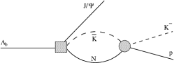
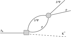
Figure 61: Mechanisms for the $\Lambda_{b}\to J/\psi K^{-}p$ reaction implementing the final state interaction

In Ref. Roca:2015tea, described in section 13, it was shown that the relevant mechanisms for the $\Lambda(1405)$ production in the decay are those depicted in Fig. 61. The upper figure shows the basic process to produce a $K^{-}p$ pair from the weak decay of the ${\Lambda_{b}}$. The $u$ and $d$ quarks of the $\Lambda_{b}$ remain as spectators in the process and carry isospin $I=0$, as in the initial state, producing, together with the $s$ quark, an $I=0$ baryon after the weak process, and hence a meson-baryon system in $I=0$ after the hadronization of the $sud$ state. The final meson-baryon state then undergoes final state interaction in coupled channels, as shown in the lower left part of Fig. 61, from where the $\Lambda(1405)$ is dynamically produced. Therefore the contribution to the $\Lambda_{b}\to J/\psi\,K^{-}p$ amplitude from the $\Lambda(1405)$ resonance is given by (see Sec. 13):

$$T^{(K^{-}p)}(M_{K^{-}p})=V_{p}\bigg{(}h_{K^{-}p}+\sum_{i}h_{i}G_{i}(M_{K^{-}p})\,t_{i\,K^{-}p}(M_{K^{-}p})\bigg{)}\,,$$ (201)

where $M_{K^{-}p}$ is the $K^{-}p$ invariant mass, $h_{i}$ are numerical $SU(3)$ factors relating the production of the different meson-baryon channels $i$ in the hadronization [see Eq. (183)], and $V_{p}$ accounts for CKM matrix elements and kinematic prefactors. Since we do not need the absolute normalization of the invariant mass distributions, the value of $V_{p}$ can be taken as appropriate, as explained below when discussing the results. In Eq. (201), $G_{i}$ represents the meson-baryon loop function and $t_{ij}$ stands for the s-wave meson-baryon unitarized scattering amplitudes from Ref. Roca:2013cca. Note that the $\Lambda(1405)$ is not included as an explicit degree of freedom but it appears dynamically in the highly non-linear dynamics involved in the unitarization procedure leading to the $t_{ij}$ amplitudes. Actually two poles are obtained for the $\Lambda(1405)$ resonance at $1352-48i$ MeV and $1419-29i$ MeV[275]. The highest mass $\Lambda(1405)$, coupling mostly to $\bar{K}N$, is the one of relevance in the present work since it is closer to the energy region of concern.

On the other hand, in Refs. Xiao:2013yca,Wu:2010vk, it was shown that the $J/\psi\,N$ final state interaction in coupled channels, considering also the $\bar{D}^{*}\Lambda_{c}$, $\bar{D}^{*}\Sigma_{c}$, $\bar{D}\Sigma^{*}_{c}$ and $\bar{D}^{*}\Sigma^{*}_{c}$, produces poles in the $J^{P}=3/2^{-}$, $I=1/2$, sector at $4334+19i\text{ MeV}$, $4417+4i\text{ MeV}$ and $4481+17i\text{ MeV}$ which couple sizeably to $J/\psi\,p$ (see table II in Ref. Xiao:2013yca). Therefore we can expect to see a resonance shape in the $J/\psi\,p$ invariant mass distribution in the $\Lambda_{b}\to J/\psi\,K^{-}p$ decay, maybe a mixture of the different poles. The mechanism for the final $J/\psi\,N$ state interaction is depicted in the lower right part of Fig. 61. The filled circle in that figure represents the final $J/\psi\,p\to J/\psi\,p$ unitarized scattering amplitude. Since the shape of this amplitude in the real axis is very close to a Breit-Wigner[298], for the numerical evaluation in the present work we can effectively account for it by using

$$t_{J/\psi\,p\to J/\psi\,p}=\frac{g^{2}_{J/\psi\,p}}{M_{J/\psi\,p}-M_{R}+i\frac{\Gamma_{R}}{2}}$$ (202)

where $M_{J/\psi\,p}$ is the $J/\psi\,p$ invariant mass and $M_{R}$ ($\Gamma_{R}$) the mass (width) of the $P_{c}(4450)^{+}$. The amplitudes in Refs.  Xiao:2013yca,Wu:2010vk provide poles from where $M_{R}$ and $\Gamma_{R}$ can be directly obtained, but we fine tune these values to the experimental results of Ref. Aaij:2015tga, $M_{R}=4449.8\text{ MeV}$ and $\Gamma_{R}=40\text{ MeV}$ which lay indeed in between the two heaviest poles obtained in Ref. Xiao:2013yca, as quoted above. In Eq. (202), $g_{J/\psi\,p}$ stands for the coupling of the dynamically generated resonance to $J/\psi\,p$, for which a range of values from about 0.5 to 1 are obtained in Refs. Xiao:2013yca,Wu:2010vk, which are genuine and non-trivial predictions of the theory.

The contribution of the $J/\psi\,p$ final state interaction to the amplitude is then

$$T^{(J/\psi\,p)}(M_{J/\psi\,p})=V_{p}\,h_{K^{-}p}G_{J/\psi\,p}(M_{J/\psi\,p})t_{J/\psi\,p\to J/\psi\,p}(M_{J/\psi\,p})\,,$$ (203)

with $G_{J/\psi\,p}$ the $J/\psi\,p$ loop function regularized by dimensional regularization as in Ref. Xiao:2013yca.

Since the main building blocks of the $P_{c}(4450)^{+}$ state in Ref. Xiao:2013yca are $\bar{D}^{*}\Sigma_{c}$ and $\bar{D}^{*}\Sigma^{*}_{c}$, in principle the main sequence to produce this baryon should be of the type $\Lambda_{b}\to K^{-}\bar{D}^{*}\Sigma^{*}_{c}\to K^{-}pJ/\psi$ (the argument that follows hold equally for $\Sigma_{c}$), where one produces $K^{-}\bar{D}^{*}\Sigma^{*}_{c}$ in the first step and the $\bar{D}^{*}\Sigma^{*}_{c}\to pJ/\psi$ transition would provide the resonant amplitude accounting for the $P_{c}(4450)^{+}$ state in the $J/\psi\,p$ spectrum. However, as discussed in the former sections and in Ref. Roca:2015dva, these alternative mechanisms are rather suppressed, and one is thus left to produce the $P_{c}(4450)^{+}$ resonance from rescattering of $J/\psi\,p$ after the primary production of $\Lambda_{b}\to J/\psi K^{-}p$ through the mechanism depicted in Fig. 61 discussed above. This feature of the reaction is important and is what allows us to relate the $P_{c}(4450)^{+}$ production with the $K^{-}p$ production, i.e, the factor $V_{p}\,h_{K^{-}p}$ enters the production of both the $\Lambda(1405)$, via Eq. (201), and of the $P_{c}(4450)^{+}$, via Eq. (203).

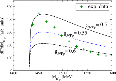
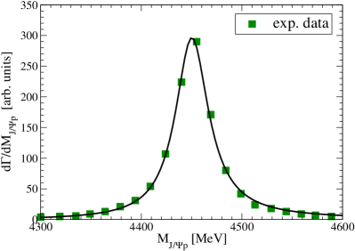
Figure 62: Results for the $K^{-}p$ and $J/\psi\,p$ invariant mass distributions compared to the data[287].

In Fig. 62 we show the results for the $K^{-}p$ and $J/\psi\,p$ invariant mass distributions compared to the experimental data of Ref. Aaij:2015tga. The absolute normalization is arbitrary but the same for both panels. In the data shown for the $K^{-}p$ mass distribution only the $\Lambda(1405)$ contribution is included, i.e., it shows the result of the $\Lambda(1405)$ component of the experimental analysis carried out in Ref. Aaij:2015tga. Therefore, in order to compare to this data set, only the amplitude of Eq. (201) is considered. Similarly, the experimental $J/\psi\,p$ mass distribution shown in Fig. 62 (right panel) only considers the contribution from the $P_{c}(4450)^{+}$ and, thus, the theoretical calculation for Fig. 62 (right panel) only includes the amplitude of Eq. (203).

The different curves are evaluated considering different values for the coupling of the $P_{c}(4450)^{+}$ to $J/\psi\,p$, ($g_{J/\psi\,p}=0.5$, 0.55 and 0.6). For each value of $g_{J/\psi\,p}$, $V_{P}$ has been normalized such that the peak of the $J/\psi\,p$ distribution agrees with experiment, and this is why there is only one curve for the $J/\psi\,p$ mass distribution. Since the higher $\Lambda(1405)$ resonance lays below the $K^{-}p$ threshold, the accumulation of strength close to threshold is due to the tail of that resonance.

The results are very sensitive to the value of the $J/\psi\,p$ coupling since the $J/\psi\,p$ partial decay width is proportional to $g_{J/\psi\,p}^{4}$. We can see in the figure that a value for the coupling of about 0.5 can account fairly for the relative strength between the $J/\psi\,p$ and $K^{-}p$ mass distributions. This value of the coupling is of the order obtained in the extended local hidden gauge unitary approach of Refs. Xiao:2013yca,Wu:2010vk which is a non-trivial output of the theoretical model since the value of this coupling is a reflection of the highly non-linear dynamics involved in the unitarization of the scattering amplitudes.

It is also worth noting that the values of $g_{J/\psi\,p}$ used, lead to a partial decay width of $P_{c}(4450)^{+}$ into $J/\psi\,p$ ($\Gamma=M_{N}g_{J/\psi\,p}^{2}~{}p_{J/\psi}/(2\pi M_{R})$) of 6.9 MeV, 8.3 MeV, 9.9 MeV, which are of the order of the experimental width, but smaller as it should be, indicating that this channel is one of the relevant ones in the decay of the $P_{c}(4450)^{+}$ state.

The fact that we can fairly reproduce the relative strength of the mass distributions with values of the coupling in the range predicted by the coupled channels unitary approach, provides support to the interpretation of the $P_{c}(4450)^{+}$ state as dynamically generated from the coupled channels considered and to the $3/2^{-}$ signature of the state.

The findings of Ref. Aaij:2015tga prompted the work of Ref. Chen:2015loa where, using a boson exchange model[304], molecular structures of $\bar{D}^{*}\Sigma_{c}$ and $\bar{D}^{*}\Sigma^{*}_{c}$ are also obtained with similarities to our earlier work of Ref. Xiao:2013yca. However, the interrelation between the $J/\psi\,p$ and $K^{-}p$ invariant mass distributions is not addressed in Ref. Chen:2015loa.

The experimental observation of Ref. Aaij:2015tga has prompted quite a few works aiming at interpreting those results with different models. It is not our purpose to discuss them here. A compilation of all these different works can be seen in Ref. Wang:2015wsa.

17 Further developments

The developments in this area in the last year have been spectacular, as shown by the different problems discussed in this review. The agreement of the results with experiment when data are available, using the approach discussed all along, has been reasonably good, and many predictions have been made for other observables that are at reach in the different facilities where the experiments have been performed. The fast experimental developments in the present facilities and the prospects for new facilities that are now under construction, make it a fertile land to apply these theoretical tools and there is much to learn.

In this last section we would like to make a very short review of other problems that we have not reviewed here and which are under study or just recently finished at the time the review was written.

In Ref. miguemarina the $B^{+}$ decay into $D_{s}^{-}K^{+}\pi^{+}$ is been studied in order to learn about the $D_{0}^{*}(2400)$ resonance.

In Ref. miguejido the $B^{+}\to\bar{D}^{0}D^{0}K^{+}$, $B^{0}\to\bar{D}^{-}D^{0}K^{+}$ and $B_{s}^{+}\to\bar{D}^{0}K^{-}\pi^{+}$ are studied. In this case the aim is to see how the $D_{s0}^{*}(2317)$ resonance is formed and learn about the $KD$ molecular structure which has been determined in lattice calculations[160].

Further developments are done in Ref. liangrio where the $B^{0}$ and $B_{s}^{0}$ decays to $J/\psi K\bar{K}$ are investigated to compare with measurements done and under analysis at LHCb.

The advent of the LHCb pentaquark experiment has also prompted the investigation of another reaction[308], $\Xi_{b}^{-}\to J/\psi K^{-}\Lambda$, where using the results of Ref. Wu:2010vk, where a hidden charm with strangeness is predicted, invariant mass distributions of $K^{-}\Lambda$ and $J/\psi\Lambda$ are evaluated and a neat peak in the $J/\psi\Lambda$ invariant mass distribution is observed.

The semileptonic $\Lambda_{c}\to\nu_{l}l^{+}\Lambda(1405)$ is addressed in Ref. ikeno.

The $B^{0}\to D^{0}\bar{D}^{0}K^{0}$ reaction is studied in Ref. daivalen in order to find evidence for a bound state of $D\bar{D}$ predicted in Ref. Gamermann:2006nm.

The $D_{s}^{+}\to\pi\pi\pi$ and $D_{s}^{+}\to\pi K\bar{K}$ reactions are investigated in Ref. jorgivan to compare with existing and coming data of LHCb.

A study is also conducted for the $B_{s}^{0}\to J/\psi f_{1}(1285)$ reaction in Ref. raqueli suggesting a model independent method to find the molecular component of resonances.

The $\Lambda_{b}\to\bar{D}_{s}\Lambda_{c}(2595)$ is also investigated in Ref. melaliang.

Finally, an incursion is also done in $B_{c}$ states[314], studying the $B_{c}\to J/\psi D_{s}^{*-}$ reaction in order to learn about the $D_{s0}^{*}(2317)$ state.

18 Conclusions

We do not want to draw conclusions on each of the many subjects dealt along this review. We can recall the basic lessons learned from this general overview. The decays studied have shown that weak decays, even when they do not conserve parity and isospin, are many times better filters for isospin or other quantities than strong or electromagnetic interactions. Selection rules as OZI, Cabibbo allowed or suppressed processes, details on the hadronization, etc…, have as a consequence that one can isolate certain quantum numbers at the end, allowing a better study of some resonances or aspects of the hadron interaction. The selection rules and the hadronization of the quarks formed in the primary step lead to pairs of hadrons with very specific weights which allow to understand the basic features of some reactions. Particular relevance have some processes where one looks for a pair of mesons which are not produced in a primary step. In this case it is only the rescattering of the primary mesons produced what gives rise to this hadron pair in the final state. Hence, the amplitude for the process is directly proportional to the scattering amplitudes of these hadrons and one gets rid of unwanted background which could blur the interpretation of the process. If resonances are produced, this gives us a way to learn about their couplings to these primary channels.

We have seen that one can learn about properties of resonances, and particularly, when one is dealing with resonances which are deemed as dynamically generated from the interaction of other hadrons, one can even find from the data the amount of molecular component.

When dealing with charmed particles, the study of these processes allows to learn about the interaction of these hadrons. In the absence of D-meson beams, unlike for pions or kaons, the study of this final state interaction is our only source of information on the interaction of the charmed hadrons.

As to light mesons, the study done here presents further evidence to that gathered from other processes, that the light scalars are generated from the interaction of pseudoscalar mesons, while the vector mesons respond very well to the standard picture of $q\bar{q}$ states. Other mesons, scalar and tensor, that are theoretically produced from the interaction of vector mesons or a vector and a pseudoscalar, were also investigated, and support for this picture was also obtained.

References

- [1] E. Klempt and A. Zaitsev, Phys. Rept. 454, 1 (2007).
- [2] V. Crede and C. A. Meyer, Prog. Part. Nucl. Phys. 63, 74 (2009).
- [3] S. Weinberg, Physica A 96, 327 (1979).
- [4] J. Gasser and H. Leutwyler, Annals Phys. 158, 142 (1984).
- [5] G. Ecker, Prog. Part. Nucl. Phys. 35, (1995).
- [6] V. Bernard, N. Kaiser and U. G. Meißner, Int. J. Mod. Phys. E 4, 193 (1995).
- [7] M. Bando, T. Kugo, S. Uehara, K. Yamawaki and T. Yanagida, Phys. Rev. Lett. 54, 1215 (1985).
- [8] M. Bando, T. Kugo and K. Yamawaki, Phys. Rept. 164, 217 (1988).
- [9] U. G. Meißner, Phys. Rept. 161, 213 (1988).
- [10] N. Kaiser, P. B. Siegel and W. Weise, Phys. Lett. B 362, 23 (1995).
- [11] E. Oset and A. Ramos, Nucl. Phys. A 635, 99 (1998).
- [12] J. A. Oller and U. G. Meißner, Phys. Lett. B 500, 263 (2001).
- [13] C. Garcia-Recio, M. F. M. Lutz and J. Nieves, Phys. Lett. B 582, 49 (2004).
- [14] C. Garcia-Recio, J. Nieves and L. L. Salcedo, Phys. Rev. D 74, 034025 (2006).
- [15] T. Hyodo, S. I. Nam, D. Jido and A. Hosaka, Phys. Rev. C 68, 018201 (2003).
- [16] Y. Ikeda, T. Hyodo and W. Weise, Nucl. Phys. A 881, 98 (2012).
- [17] D. Jido, J. A. Oller, E. Oset, A. Ramos and U. G. Meißner, Nucl. Phys. A 725, 181 (2003).
- [18] B. Borasoy, R. Nissler and W. Weise, Eur. Phys. J. A 25, 79 (2005).
- [19] J. A. Oller, J. Prades and M. Verbeni, Phys. Rev. Lett. 95, 172502 (2005).
- [20] J. A. Oller, Eur. Phys. J. A 28, 63 (2006).
- [21] B. Borasoy, U. G. Meißner and R. Nissler, Phys. Rev. C 74, 055201 (2006).
- [22] T. Hyodo, D. Jido and A. Hosaka, Phys. Rev. C 78, 025203 (2008).
- [23] M. Mai and U. G. Meißner, Eur. Phys. J. A 51, 30 (2015).
- [24] J. A. Oller and E. Oset, Nucl. Phys. A 620, 438 (1997) [Erratum-ibid. A 652, 407 (1999)].
- [25] J. A. Oller, E. Oset and J. R. Pelaez, Phys. Rev. D 59, 074001 (1999) [Erratum-ibid. D 60, 099906 (1999)] [Erratum-ibid. D 75, 099903 (2007)].
- [26] N. Kaiser, Eur. Phys. J. A 3, 307 (1998).
- [27] M. P. Locher, V. E. Markushin and H. Q. Zheng, Eur. Phys. J. C 4, 317 (1998).
- [28] J. Nieves and E. Ruiz Arriola, Nucl. Phys. A 679, 57 (2000).
- [29] J. R. Pelaez and G. Rios, Phys. Rev. Lett. 97, 242002 (2006).
- [30] M. Albaladejo and J. A. Oller, Phys. Rev. Lett. 101, 252002 (2008).
- [31] M. Albaladejo and B. Moussallam, Eur. Phys. J. C 75, 488 (2015).
- [32] J. R. Pelaez, arXiv:1510.00653 [hep-ph].
- [33] D. Gamermann, E. Oset, D. Strottman and M. J. Vicente Vacas, Phys. Rev. D 76, 074016 (2007).
- [34] L. Castillejo, R. H. Dalitz and F. J. Dyson, Phys. Rev. 101, 453 (1956).
- [35] E. van Beveren, T. A. Rijken, K. Metzger, C. Dullemond, G. Rupp and J. E. Ribeiro, Z. Phys. C 30, 615 (1986).
- [36] N. A. Tornqvist and M. Roos, Phys. Rev. Lett. 76, 1575 (1996).
- [37] A. H. Fariborz, R. Jora and J. Schechter, Phys. Rev. D 79, 074014 (2009).
- [38] A. H. Fariborz, N. W. Park, J. Schechter and M. Naeem Shahid, Phys. Rev. D 80, 113001 (2009).
- [39] R. Aaij et al. [LHCb Collaboration], Phys. Lett. B 698, 115 (2011).
- [40] J. Li et al. [Belle Collaboration], Phys. Rev. Lett. 106, 121802 (2011).
- [41] T. Aaltonen et al. [CDF Collaboration], Phys. Rev. D 84, 052012 (2011).
- [42] V. M. Abazov et al. [D0 Collaboration], Phys. Rev. D 85, 011103 (2012).
- [43] R. Aaij et al. [LHCb Collaboration], Phys. Rev. D 86, 052006 (2012).
- [44] R. Aaij et al. [LHCb Collaboration], Phys. Rev. D 87, 052001 (2013).
- [45] R. Aaij et al. [LHCb Collaboration], Phys. Rev. D 89, 092006 (2014).
- [46] R. Aaij et al. [LHCb Collaboration], Phys. Rev. D 90, 012003 (2014).
- [47] W. H. Liang and E. Oset, Phys. Lett. B 737, 70 (2014).
- [48] S. Stone and L. Zhang, Phys. Rev. Lett. 111, 062001 (2013).
- [49] M. Kobayashi and T. Maskawa, Prog. Theor. Phys. 49, 652 (1973).
- [50] L. Wolfenstein, Phys. Rev. Lett. 51, 1945 (1983).
- [51] G. Buchalla, A. J. Buras and M. E. Lautenbacher, Rev. Mod. Phys. 68, 1125 (1996).
- [52] B. El-Bennich, A. Furman, R. Kaminski, L. Lesniak, B. Loiseau and B. Moussallam, Phys. Rev. D 79, 094005 (2009); [Erratum-ibid. D 83, 039903 (2011)].
- [53] O. Leitner, J.-P. Dedonder, B. Loiseau and R. Kaminski, Phys. Rev. D 81, 094033 (2010); [Erratum-ibid. D 82, 119906 (2010)].
- [54] A. Bramon, A. Grau and G. Pancheri, Phys. Lett. B 283, 416 (1992).
- [55] L. Roca, J. E. Palomar and E. Oset, Phys. Rev. D 70, 094006 (2004).
- [56] D. Gamermann, E. Oset and B. S. Zou, Eur. Phys. J. A 41, 85 (2009).
- [57] J. A. Oller, E. Oset and J. E. Palomar, Phys. Rev. D 63, 114009 (2001).
- [58] J. A. Oller and E. Oset, Phys. Rev. D 60, 074023 (1999)
- [59] J. Yamagata-Sekihara, J. Nieves and E. Oset, Phys. Rev. D 83, 014003 (2011)
- [60] W. H. Liang, J. J. Xie and E. Oset, arXiv:1510.03175 [hep-ph]. Eur. Phys. J. C, in print.
- [61] J. T. Daub, C. Hanhart and B. Kubis, arXiv:1508.06841 [hep-ph].
- [62] J. W. Li, D. S. Du and C. D. Lu, Eur. Phys. J. C 72, 2229 (2012).
- [63] W. Ochs, J. Phys. G 40, 043001 (2013).
- [64] X. W. Kang, B. Kubis, C. Hanhart and U. G. Meißner, Phys. Rev. D 89, 053015 (2014).
- [65] C. Albertus, E. Hernandez and J. Nieves, Phys. Lett. B 690, 265 (2010) [arXiv:1004.3154 [hep-ph]].
- [66] C. Albertus, E. Hernandez and J. Nieves, Phys. Lett. B 704, 499 (2011) [arXiv:1108.1296 [hep-ph]].
- [67] C. Albertus, E. Hernandez and J. Nieves, Phys. Rev. D 85, 094035 (2012) [arXiv:1202.4861 [hep-ph]].
- [68] C. Albertus, E. Hernández and J. Nieves, Phys. Rev. D 90, no. 1, 013017 (2014) [Phys. Rev. D 90, no. 7, 079906 (2014)] [arXiv:1406.7782 [hep-ph]].
- [69] C. Albertus, E. Hernández, C. Hidalgo-Duque and J. Nieves, Phys. Lett. B 738, 144 (2014) [arXiv:1404.1001 [hep-ph]].
- [70] A. Furman, R. Kaminski, L. Lesniak and B. Loiseau, Phys. Lett. B 622, 207 (2005) [hep-ph/0504116].
- [71] B. El-Bennich, A. Furman, R. Kaminski, L. Lesniak and B. Loiseau, Phys. Rev. D 74, 114009 (2006) [hep-ph/0608205].
- [72] H. Y. Cheng, C. K. Chua and K. C. Yang, Phys. Rev. D 73, 014017 (2006) [hep-ph/0508104].
- [73] B. El-Bennich, O. Leitner, J. -P. Dedonder and B. Loiseau, Phys. Rev. D 79, 076004 (2009) [arXiv:0810.5771 [hep-ph]].
- [74] O. Leitner, J. -P. Dedonder, B. Loiseau and B. El-Bennich, Phys. Rev. D 82, 076006 (2010) [arXiv:1003.5980 [hep-ph]].
- [75] D. Delepine, J. L. Lucio M. and C. A. Ramirez, Eur. Phys. J. C 45, 693 (2006) [hep-ph/0501022].
- [76] P. Colangelo, F. De Fazio and W. Wang, Phys. Rev. D 81, 074001 (2010).
- [77] M. Sayahi and H. Mehraban, Phys. Scripta 88, 035101 (2013).
- [78] I. Bediaga, F. S. Navarra and M. Nielsen, Phys. Lett. B 579, 59 (2004).
- [79] H. W. Ke, X. Q. Li and Z. T. Wei, Phys. Rev. D 80, 074030 (2009) [arXiv:0907.5465 [hep-ph]].
- [80] N. N. Achasov and A. V. Kiselev, Phys. Rev. D 86, 114010 (2012) [arXiv:1206.5500 [hep-ph]].
- [81] A. H. Fariborz, R. Jora, J. Schechter and M. Naeem Shahid, Phys. Rev. D 84, 094024 (2011).
- [82] A. H. Fariborz, R. Jora, J. Schechter and M. N. Shahid, Int. J. Mod. Phys. A 30, 1550012 (2015).
- [83] W. Wang and C. D. Lu, Phys. Rev. D 82, 034016 (2010).
- [84] Y. J. Shi and W. Wang, arXiv:1507.07692 [hep-ph].
- [85] U. G. Meißner and W. Wang, Phys. Lett. B 730, 336 (2014).
- [86] W. Wang and R. L. Zhu, Phys. Lett. B 743, 467 (2015).
- [87] U. G. Meißner and W. Wang, JHEP 1401, 107 (2014).
- [88] W. F. Wang, H. N. Li, W. Wang and C. D. Lu, Phys. Rev. D 91, 094024 (2015).
- [89] M. Döring, U. G. Meißner and W. Wang, JHEP 1310, 011 (2013).
- [90] J. Gasser and H. Leutwyler, Nucl. Phys. B 250, 517 (1985).
- [91] A. V. Manohar and M. B. Wise, Camb. Monogr. Part. Phys. Nucl. Phys. Cosmol. 10, 1 (2000).
- [92] J. R. Pelaez, Phys. Rev. Lett. 92, 102001 (2004).
- [93] F. Aceti and E. Oset, Phys. Rev. D 86, 014012 (2012).
- [94] C. W. Xiao, F. Aceti and M. Bayar, Eur. Phys. J. A 49, 22 (2013).
- [95] K. A. Olive et al. [Particle Data Group Collaboration], Chin. Phys. C 38, 090001 (2014).
- [96] X. Liu, W. Wang and Y. Xie, Phys. Rev. D 89, 094010 (2014).
- [97] L. Zhang and S. Stone, Phys. Lett. B 719, 383 (2013).
- [98] M. Bayar, W. H. Liang and E. Oset, Phys. Rev. D 90, 114004 (2014).
- [99] M. Ablikim et al. [BES Collaboration], Phys. Lett. B 598, 149 (2004).
- [100] C. B. Li, E. Oset and M. J. Vicente Vacas, Phys. Rev. C 69, 015201 (2004).
- [101] M.J. Yan and W. H. Liang, to be published.
- [102] N. Wu, hep-ex/0104050.
- [103] J. E. Augustin et al. [DM2 Collaboration], Nucl. Phys. B 320, 1 (1989).
- [104] L. Roca, J. E. Palomar, E. Oset and H. C. Chiang, Nucl. Phys. A 744, 127 (2004)
- [105] K. Abe et al. [Belle Collaboration], Phys. Lett. B 538, 11 (2002).
- [106] E. M. Aitala et al. [E791 Collaboration], Phys. Rev. Lett. 89, 121801 (2002).
- [107] J. M. Link et al. [FOCUS Collaboration], Phys. Lett. B 653, 1 (2007).
- [108] J. J. Xie, L. R. Dai and E. Oset, Phys. Lett. B 742, 363 (2015).
- [109] P. Rubin et al. [CLEO Collaboration], Phys. Rev. Lett. 93, 111801 (2004).
- [110] H. Muramatsu et al. [CLEO Collaboration], Phys. Rev. Lett. 89, 251802 (2002); [Erratum-ibid. 90, 059901 (2003)].
- [111] L. L. Chau, Phys. Rept. 95, 1 (1983).
- [112] L. L. Chau and H. Y. Cheng, Phys. Rev. D 36, 137 (1987).
- [113] H. Y. Cheng and C. W. Chiang, Phys. Rev. D 81, 074031 (2010).
- [114] J.-P. Dedonder, R. Kaminski, L. Lesniak and B. Loiseau, Phys. Rev. D 89, 094018 (2014).
- [115] A. Kuzmin et al. (Belle Collaboration), Phys. Rev. D 76, 012006 (2007).
- [116] R. Aaij et al. (LHCb Collaboration), Phys. Rev. Lett. 109, 131801 (2012).
- [117] W. H. Liang, J. J. Xie and E. Oset, Phys. Rev. D 92, 034008 (2015).
- [118] F. K. Guo, R. G. Ping, P. N. Shen, H. C. Chiang and B. S. Zou, Nucl. Phys. A 773, 78 (2006).
- [119] J. P. Lees et al. (BaBar Collaboration), Phys. Rev. D 84, 112007 (2011); 87, 039901(E) (2013).
- [120] S. Blyth et al. (BELLE Collaboration), Phys. Rev. D 74, 092002 (2006).
- [121] R. Aaij et al. (LHCb Collaboration), Phys. Rev. D 90, 072003 (2014).
- [122] R. Aaij et al. (LHCb Collaboration), Phys. Rev. D 87, 112009 (2013).
- [123] R. Aaij et al. (LHCb Collaboration), Phys. Lett. B 706, 32 (2011).
- [124] Tim Gershon and LHCb Collaboration, (private communication).
- [125] R. Molina, D. Nicmorus and E. Oset, Phys. Rev. D 78, 114018 (2008) [arXiv:0809.2233 [hep-ph]].
- [126] L. S. Geng and E. Oset, Phys. Rev. D 79, 074009 (2009).
- [127] J. J. Xie and E. Oset, Phys. Rev. D 90, 094006 (2014).
- [128] A. Martinez Torres, L. S. Geng, L. R. Dai, B. X. Sun, E. Oset and B. S. Zou, Phys. Lett. B 680, 310 (2009).
- [129] L. S. Geng, F. K. Guo, C. Hanhart, R. Molina, E. Oset and B. S. Zou, Eur. Phys. J. A 44, 305 (2010).
- [130] R. Aaij et al. [LHCb Collaboration], Phys. Rev. Lett. 108, 151801 (2012).
- [131] R. Aaij et al. [LHCb Collaboration], Phys. Lett. B 713, 378 (2012).
- [132] E. E. Kolomeitsev and M. F. M. Lutz, Phys. Lett. B 582, 39 (2004).
- [133] F. K. Guo, P. N. Shen, H. C. Chiang, R. G. Ping and B. S. Zou, Phys. Lett. B 641, 278 (2006).
- [134] F. K. Guo, C. Hanhart and U. G. Meißner, Eur. Phys. J. A 40, 171 (2009).
- [135] M. Cleven, F. K. Guo, C. Hanhart and U. G. Meißner, Eur. Phys. J. A 47, 19 (2011).
- [136] M. Cleven, H. W. Griesshammer, F. K. Guo, C. Hanhart and U. G. Meißner, Eur. Phys. J. A 50, 149 (2014).
- [137] B. Aubert et al. [BaBar Collaboration], Phys. Rev. Lett. 90 (2003) 242001.
- [138] B. Aubert et al. [BaBar Collaboration], Phys. Rev. D 69 (2004) 031101.
- [139] CLEO Coll., D. Besson et al., Phys. Rev. D68, 032002 (2003).
- [140] BELLE Coll., P. Krokovny et al., Phys. Rev. Lett. 91, 262002 (2003).
- [141] FOCUS Coll., E.W. Vaandering, hep-ex/0406044.
- [142] S. Godfrey and N. Isgur, Phys. Rev. D32, 189 (1985).
- [143] S. Godfrey and R. Kokoshi, Phys. Rev. D43, 1679 (1991).
- [144] Y. B. Dai, C. S. Huang, C. Liu and S. L. Zhu, Phys. Rev. D68, 114011 (2003).
- [145] G.S. Bali, Phys. Rev. D68, 071501(R) (2003).
- [146] A. Dougall et al. [UKQCD Collaboration], Phys. Lett. B569, 41 (2003).
- [147] A. Hayashigaki and K. Terasaki, hep-ph/0411285.
- [148] S. Narison, Phys. Lett. B605, 319 (2005).
- [149] T. Barnes, F.E. Close and H.J. Lipkin, Phys. Rev. D68, 054006 (2003).
- [150] A.P. Szczepaniak, Phys. Lett. B567, 23 (2003).
- [151] E. van Beveren and G. Rupp, Phys. Rev. Lett. 91, 012003 (2003).
- [152] H.-Y. Cheng and W.-S. Hou, Phys. Lett. B566, 193 (2003).
- [153] K. Terasaki, Phys. Rev. D68, 011501(R) (2003).
- [154] L. Maiani, F. Piccinini, A.D. Polosa, V. Riquer, Phys. Rev. D71, 014028 (2005).
- [155] M. E. Bracco, A. Lozea, R. D. Matheus, F. S. Navarra and M. Nielsen, Phys. Lett. B 624, 217 (2005).
- [156] T. Browder, S. Pakvasa and A.A. Petrov, Phys. Lett. B578, 365 (2004).
- [157] D. Mohler, C. B. Lang, L. Leskovec, S. Prelovsek and R. M. Woloshyn, Phys. Rev. Lett. 111, 222001 (2013).
- [158] L. Liu, K. Orginos, F. K. Guo, C. Hanhart and U. G. Meißner, Phys. Rev. D 87, 014508 (2013).
- [159] C. B. Lang, L. Leskovec, D. Mohler, S. Prelovsek and R. M. Woloshyn, Phys. Rev. D 90, 034510 (2014).
- [160] A. Martínez Torres, E. Oset, S. Prelovsek and A. Ramos, JHEP 1505 (2015) 153.
- [161] S. Weinberg, Phys. Rev. 137, B672 (1965).
- [162] V. Baru, J. Haidenbauer, C. Hanhart, Y. Kalashnikova and A. E. Kudryavtsev, Phys. Lett. B 586, 53 (2004).
- [163] M. Altenbuchinger, L.-S. Geng and W. Weise, Phys. Rev. D 89, no. 1, 014026 (2014) [arXiv:1309.4743 [hep-ph]].
- [164] M. Altenbuchinger and L. S. Geng, Phys. Rev. D 89, no. 5, 054008 (2014) [arXiv:1310.5224 [hep-ph]].
- [165] J. P. Lees et al. [BaBar Collaboration], Phys. Rev. D 91, 052002 (2015).
- [166] M. Albaladejo, M. Nielsen and E. Oset, Phys. Lett. B 746, 305 (2015).
- [167] D. Gamermann, J. Nieves, E. Oset and E. Ruiz Arriola, Phys. Rev. D 81, 014029 (2010).
- [168] T. Sekihara, T. Hyodo and D. Jido, PTEP 2015, 063D04 (2015).
- [169] T. Barnes, Int. J. Mod. Phys. A 21, 5583 (2006).
- [170] D. M. Asner, T. Barnes, J. M. Bian, I. I. Bigi, N. Brambilla, I. R. Boyko, V. Bytev and K. T. Chao et al., Int. J. Mod. Phys. A 24, S1 (2009).
- [171] S. Godfrey and S. L. Olsen, Ann. Rev. Nucl. Part. Sci. 58, 51 (2008).
- [172] S. Cheng-Ping [Belle Collaboration], Chin. Phys. C 34, 615 (2010).
- [173] S. L. Olsen, Prog. Theor. Phys. Suppl. 193, 38 (2012).
- [174] S. Lange et al. [PANDA Collaboration], arXiv:1311.7597 [hep-ex].
- [175] X. Liu, Chin. Sci. Bull. 59, 3815 (2014).
- [176] Y. P. Guo, EPJ Web Conf. 81, 01008 (2014).
- [177] S. L. Olsen, Front. Phys. 10, 101401 (2015).
- [178] P. G. Ortega, D. R. Entem and F. Fernandez, J. Phys. G 40, 065107 (2013).
- [179] J. Vijande and A. Valcarce, Phys. Lett. B 736, 325 (2014).
- [180] A. Esposito, A. L. Guerrieri, F. Piccinini, A. Pilloni and A. D. Polosa, Int. J. Mod. Phys. A 30, 1530002 (2014).
- [181] T. Branz, T. Gutsche and V. E. Lyubovitskij, Phys. Rev. D 80, 054019 (2009).
- [182] T. Branz, T. Gutsche and V. E. Lyubovitskij, Phys. Rev. D 82, 054025 (2010).
- [183] Y. C. Yang, Z. Xia and J. Ping, Phys. Rev. D 81, 094003 (2010).
- [184] Y. Dong, A. Faessler, T. Gutsche and V. E. Lyubovitskij, J. Phys. G 40, 015002 (2013).
- [185] Q. Wang, C. Hanhart and Q. Zhao, Phys. Rev. Lett. 111, 132003 (2013).
- [186] M. Cleven, Q. Wang, F. K. Guo, C. Hanhart, U. G. Meißner and Q. Zhao, Phys. Rev. D 87, 074006 (2013).
- [187] Q. Wang, M. Cleven, F. K. Guo, C. Hanhart, U. G. Mei Ãner, X. G. Wu and Q. Zhao, Phys. Rev. D 89, 034001 (2014).
- [188] F. Aceti, M. Bayar, J. M. Dias and E. Oset, Eur. Phys. J. A 50, 103 (2014).
- [189] F. Aceti, M. Bayar, E. Oset, A. Martinez Torres, K. P. Khemchandani, J. M. Dias, F. S. Navarra and M. Nielsen, Phys. Rev. D 90, 016003 (2014).
- [190] J. Nieves and M. P. Valderrama, Phys. Rev. D 86, 056004 (2012).
- [191] C. Hidalgo-Duque, J. Nieves and M. P. Valderrama, Phys. Rev. D 87, 076006 (2013).
- [192] M. Albaladejo, F. K. Guo, C. Hidalgo-Duque, J. Nieves and M. P. Valderrama, arXiv:1504.00861 [hep-ph].
- [193] M. Nielsen, F. S. Navarra and S. H. Lee, Phys. Rept. 497, 41 (2010).
- [194] K. P. Khemchandani, A. Martinez Torres, M. Nielsen and F. S. Navarra, Phys. Rev. D 89, 014029 (2014).
- [195] M. Nielsen and F. S. Navarra, Mod. Phys. Lett. A 29, 1430005 (2014).
- [196] Y. Dong, A. Faessler, T. Gutsche and V. E. Lyubovitskij, Phys. Rev. D 88, 014030 (2013).
- [197] L. Ma, X. H. Liu, X. Liu and S. L. Zhu, Phys. Rev. D 91, 034032 (2015).
- [198] W. H. Liang, R. Molina and E. Oset, Eur. Phys. J. A 44, 479 (2010).
- [199] T. Branz, T. Gutsche and V. E. Lyubovitskij, Phys. Rev. D 82, 054010 (2010).
- [200] F. Aceti, R. Molina and E. Oset, Phys. Rev. D 86, 113007 (2012).
- [201] L. Ma, Z. F. Sun, X. H. Liu, W. Z. Deng, X. Liu and S. L. Zhu, Phys. Rev. D 90, 034020 (2014).
- [202] Y. Dong, A. Faessler, T. Gutsche and V. E. Lyubovitskij, Phys. Rev. D 90, 074032 (2014).
- [203] F. K. Guo, C. Hanhart, Y. S. Kalashnikova, U.-G. Meißner and A. V. Nefediev, Phys. Lett. B 742, 394 (2015).
- [204] E. S. Swanson, Phys. Rev. D 91, 034009 (2015).
- [205] F. K. Guo, C. Hanhart, Q. Wang and Q. Zhao, Phys. Rev. D 91, 051504 (2015).
- [206] A. P. Szczepaniak, Phys. Lett. B 747, 410 (2015)
- [207] S. L. Zhu, Int. J. Mod. Phys. E 17, 283 (2008).
- [208] N. Brambilla, S. Eidelman, B. K. Heltsley, R. Vogt, G. T. Bodwin, E. Eichten, A. D. Frawley and A. B. Meyer et al., Eur. Phys. J. C 71, 1534 (2011).
- [209] N. Drenska, R. Faccini, F. Piccinini, A. Polosa, F. Renga and C. Sabelli, Riv. Nuovo Cim. 33, 633 (2010).
- [210] W. H. Liang, J. J. Xie, E. Oset, R. Molina and M. Döring, Eur. Phys. J. A 51, 58 (2015).
- [211] R. Molina and E. Oset, Phys. Rev. D 80, 114013 (2009).
- [212] H. Nagahiro, L. Roca, A. Hosaka and E. Oset, Phys. Rev. D 79, 014015 (2009).
- [213] K. Abe et al. [Belle Collaboration], Phys. Rev. Lett. 94, 182002 (2005).
- [214] S. Uehara et al. [Belle Collaboration], Phys. Rev. Lett. 96, 082003 (2006).
- [215] P. Pakhlov et al. [Belle Collaboration], Phys. Rev. Lett. 100, 202001 (2008).
- [216] T. Gutsche, T. Branz, A. Faessler, I. W. Lee and V. E. Lyubovitskij, Chin. Phys. C 34, 1185 (2010).
- [217] Z. G. Wang, Eur. Phys. J. C 74, 2963 (2014).
- [218] X. Liu and S. L. Zhu, Phys. Rev. D 80, 017502 (2009) [Erratum-ibid. D 85, 019902 (2012)].
- [219] W. H. Liang, C. W. Xiao and E. Oset, Phys. Rev. D 89, 054023 (2014).
- [220] F. S. Navarra, M. Nielsen, E. Oset and T. Sekihara, Phys. Rev. D 92, 014031 (2015).
- [221] E. Braaten, Y. Jia and T. Mehen, Phys. Rev. D 66, 014003 (2002).
- [222] E. Braaten, Y. Jia and T. Mehen, Phys. Rev. Lett. 89, 122002 (2002).
- [223] E. Braaten and M. Kusunoki, Phys. Rev. D 69, 114012 (2004).
- [224] E. Braaten, M. Kusunoki and S. Nussinov, Phys. Rev. Lett. 93, 162001 (2004).
- [225] T. Hyodo, D. Jido and A. Hosaka, Phys. Rev. C 85, 015201 (2012).
- [226] T. Hyodo, Int. J. Mod. Phys. A 28, 1330045 (2013).
- [227] T. Sekihara, T. Hyodo and D. Jido, Phys. Rev. C 83, 055202 (2011).
- [228] M. Q. Huang, Phys. Rev. D 69, 114015 (2004).
- [229] T. M. Aliev and M. Savci, Phys. Rev. D 73, 114010 (2006).
- [230] R. H. Li, C. D. Lu and Y. M. Wang, Phys. Rev. D 80, 014005 (2009).
- [231] S. M. Zhao, X. Liu and S. J. Li, Eur. Phys. J. C 51, 601 (2007).
- [232] J. Segovia et al., Phys. Rev. D 84, 094029 (2011).
- [233] C. Albertus, Phys. Rev. D 89, 065042 (2014).
- [234] M. Ablikim et al. [BES Collaboration], Eur. Phys. J. C 47, 31 (2006).
- [235] M. Ablikim et al. [BES Collaboration], Eur. Phys. J. C 47, 39 (2006).
- [236] J. M. Link et al. [FOCUS Collaboration], Phys. Lett. B 598, 33 (2004).
- [237] J. M. Link et al. [FOCUS Collaboration], Phys. Lett. B 637, 32 (2006).
- [238] B. Aubert et al. [BaBar Collaboration], Phys. Rev. D 78, 051101 (2008).
- [239] P. del Amo Sanchez et al. [BaBar Collaboration], Phys. Rev. D 83, 072001 (2011).
- [240] J. Yelton et al. [CLEO Collaboration], Phys. Rev. D 80, 052007 (2009).
- [241] K. M. Ecklund et al. [CLEO Collaboration], Phys. Rev. D 80, 052009 (2009).
- [242] L. Martin et al. [CLEO Collaboration], Phys. Rev. D 84, 012005 (2011).
- [243] J. Yelton et al. [CLEO Collaboration], Phys. Rev. D 84, 032001 (2011).
- [244] S. Dobbs et al. [CLEO Collaboration], Phys. Rev. Lett. 110, 131802 (2013).
- [245] T. Sekihara and E. Oset, Phys. Rev. D 92, no. 5, 054038 (2015) [arXiv:1507.02026 [hep-ph]].
- [246] J. Hietala, D. Cronin-Hennessy, T. Pedlar and I. Shipsey, Phys. Rev. D 92, 012009 (2015).
- [247] R. Dalitz and S. Tuan, Annals Phys. 10, 307 (1960).
- [248] R. H. Dalitz, T. C. Wong and G. Rajasekaran, Phys. Rev. 153, 1617 (1967).
- [249] E. A. Veit, B. K. Jennings, R. C. Barrett and A. W. Thomas, Phys. Lett. B 137, 415 (1984).
- [250] N. Kaiser, P. B. Siegel and W. Weise, Nucl. Phys. A 594, 325 (1995).
- [251] N. Kaiser, T. Waas and W. Weise, Nucl. Phys. A 612, 297 (1997).
- [252] M. F. M. Lutz and E. E. Kolomeitsev, Nucl. Phys. A 700, 193 (2002).
- [253] E. Oset, A. Ramos and C. Bennhold, Phys. Lett. B 527, 99 (2002) [Phys. Lett. B 530, 260 (2002)].
- [254] C. Garcia-Recio, J. Nieves, E. Ruiz Arriola and M. J. Vicente Vacas, Phys. Rev. D 67, 076009 (2003).
- [255] P. J. Fink, Jr., G. He, R. H. Landau and J. W. Schnick, Phys. Rev. C 41, 2720 (1990).
- [256] D. W. Thomas, A. Engler, H. E. Fisk and R. W. Kraemer, Nucl. Phys. B 56, 15 (1973).
- [257] R. J. Hemingway, Nucl. Phys. B 253, 742 (1985).
- [258] M. Niiyama et al., Phys. Rev. C 78, 035202 (2008).
- [259] S. Prakhov et al. [Crystall Ball Collaboration], Phys. Rev. C 70, 034605 (2004).
- [260] K. Moriya et al. [CLAS Collaboration], AIP Conf. Proc. 1441, 296 (2012).
- [261] K. Moriya et al. [CLAS Collaboration], Phys. Rev. C 87, 035206 (2013).
- [262] I. Zychor et al., Phys. Lett. B 660, 167 (2008).
- [263] G. Agakishiev et al. [HADES Collaboration], Phys. Rev. C 87, 025201 (2013).
- [264] V. K. Magas, E. Oset and A. Ramos, Phys. Rev. Lett. 95, 052301 (2005).
- [265] O. Braun et al., Nucl. Phys. B 129, 1 (1977).
- [266] D. Jido, E. Oset and T. Sekihara, Eur. Phys. J. A 42, 257 (2009).
- [267] K. Miyagawa and J. Haidenbauer, Phys. Rev. C 85, 065201 (2012).
- [268] D. Jido, E. Oset and T. Sekihara, Eur. Phys. J. A 49, 95 (2013).
- [269] X. L. Ren, E. Oset, L. Alvarez-Ruso and M. J. Vicente Vacas, Phys. Rev. C 91, 045201 (2015).
- [270] L. Roca, M. Mai, E. Oset and U. G. Meißner, Eur. Phys. J. C 75, 218 (2015).
- [271] R. Aaij et al. [LHCb Collaboration], JHEP 1407, 103 (2014).
- [272] F. E. Close, “An Introduction to Quarks and Partons,” Academic Press, London 1979, 481p
- [273] M. Mai and U. G. Meißner, Nucl. Phys. A 900, 51 (2013).
- [274] L. Roca and E. Oset, Phys. Rev. C 87, 055201 (2013).
- [275] L. Roca and E. Oset, Phys. Rev. C 88, 055206 (2013).
- [276] T. A. Aaltonen et al. [CDF Collaboration], Phys. Rev. Lett. 113, 242001 (2014).
- [277] G. Burgun et al., Nucl. Phys. B 8, 447 (1968).
- [278] J. R. Carlson, et al., Phys. Rev. D 7, 2533 (1973).
- [279] P. M. Dauber, et al., Phys. Rev. 179, 1262 (1969).
- [280] M. Haque et al., Phys. Rev. 152, 1148 (1966).
- [281] G. W. London, et al., Phys. Rev. 143, 1034 (1966).
- [282] T. G. Trippe, P. E. Schlein, Phys. Rev. 158, 1334 (1967).
- [283] W. P. Trower, et al., Phys. Rev. 170, 1207 (1968).
- [284] A. Feijoo, V. K. Magas and A. Ramos, Phys. Rev. C 92, 015206 (2015).
- [285] T. Aaltonen et al. [CDF Collaboration], Phys. Rev. Lett. 106, 121804 (2011).
- [286] R. Aaij et al. [LHCb Collaboration], Phys. Rev. Lett. 111, 102003 (2013).
- [287] R. Aaij et al. [LHCb Collaboration], Phys. Rev. Lett. 115, 072001 (2015).
- [288] A. Feijoo, V. K. Magas, A. Ramos and E. Oset, Phys. Rev. D 92, 076015 (2015).
- [289] R. L. Jaffe, Phys. Rept. 409, 1 (2005).
- [290] T. Hyodo and M. Oka, Phys. Rev. C 84, 035201 (2011).
- [291] K. Miyahara, T. Hyodo and E. Oset, arXiv:1508.04882 [nucl-th].
- [292] T. Hyodo and D. Jido, Prog. Part. Nucl. Phys. 67, 55 (2012).
- [293] M. Bazzi et al., Phys. Lett. B 704, 113 (2011).
- [294] M. Bazzi et al., Nucl. Phys. A 881, 88 (2012).
- [295] Y. Ikeda, T. Hyodo and W. Weise, Phys. Lett. B 706, 63 (2011).
- [296] J. C. Nacher, E. Oset, H. Toki and A. Ramos, Phys. Lett. B 455, 55 (1999).
- [297] K. Moriya et al. [CLAS Collaboration], Phys. Rev. C 88, 045201 (2013) [Phys. Rev. C 88, no. 4, 049902 (2013)].
- [298] C. W. Xiao, J. Nieves and E. Oset, Phys. Rev. D 88, 056012 (2013).
- [299] C. Garcia-Recio, J. Nieves, O. Romanets, L. L. Salcedo and L. Tolos, Phys. Rev. D 87, 074034 (2013).
- [300] T. Uchino, W. H. Liang and E. Oset, arXiv:1504.05726 [hep-ph].
- [301] J. J. Wu, R. Molina, E. Oset and B. S. Zou, Phys. Rev. C 84, 015202 (2011).
- [302] L. Roca, J. Nieves and E. Oset, Phys. Rev. D 92, 094003 (2015).
- [303] R. Chen, X. Liu, X. Q. Li and S. L. Zhu, Phys. Rev. Lett. 115, 132002 (2015).
- [304] Z. C. Yang, Z. F. Sun, J. He, X. Liu and S. L. Zhu, Chin. Phys. C 36, 6 (2012).
- [305] Z. G. Wang, arXiv:1509.06436 [hep-ph].
- [306] M. Albaladejo, M. Nielsen and E. Oset
- [307] M. Albaladejo, D. Jido, J. Nieves and E. Oset
- [308] H. X. Chen, L. S. Geng, W. H. Liang, E. Oset, E. Wang and J. J. Xie, arXiv:1510.01803 [hep-ph].
- [309] N. Ikeno and E. Oset, arXiv:1510.02406 [hep-ph].
- [310] L. R. Dai, J. J. Xie and E. Oset
- [311] J. M. Dias, F. Navarra, M. Nielsen and E. Oset
- [312] R. Molina, M. Döring and E. Oset
- [313] M. Bayar, W. H. Liang and E. Oset
- [314] Z. F. Sun, M. Bayar, P. Fernandez-Soler and E. Oset, arXiv:1510.06316 [hep-ph].