Initial conditions from the shadowed Glauber model for Pb+Pb at $\sqrt{s_{\rm NN}}=2.76$ TeV

Abstract

We study the initial conditions for Pb+Pb collisions at $\sqrt{s_{\rm NN}}=2.76$ TeV using the two component Monte-Carlo Glauber model with shadowing of the nucleons in the interior by the leading ones. The model parameters are fixed by comparing to the multiplicity data of p+Pb and Pb+Pb at $\sqrt{s_{\rm NN}}=5.02$ and $2.76$ TeV respectively. We then compute the centrality dependence of the eccentricities upto the fourth order as well as their event by event distributions. The inclusion of shadowing brings the Monte-Carlo Glauber model predictions in agreement with data as well as with results from other dynamical models of initial conditions based on gluon saturation at high energy nuclear collisions. Further, we find that the shadowed Glauber model provides the desired relative magnitude between the ellipticity and triangularity of the initial energy distribution required to explain the data on the even and odd flow harmonics $v_{2}$ and $v_{3}$ respectively at the LHC.

I Introduction

One of the most important ingredients in understanding the evolution of matter formed in heavy ion collisions (HIC) is its initial condition (IC). Currently there are several models of IC available with varying degrees of success in explaining the data Bialas et al. (1976); Eskola et al. (2000); Kharzeev and Nardi (2001); Kharzeev et al. (2005); Hirano et al. (2006); Miller et al. (2007); Broniowski et al. (2009); Schenke et al. (2012); Gale et al. (2013); Rybczynski et al. (2013); Goldschmidt et al. (2015); Niemi et al. (2015). The Monte-Carlo based IC models generate the event by event (E/E) fluctuations in observables which can be compared to those measured in experiments. Most of these models share the first step- sampling the positions of the constituent nucleons of the two colliding nuclei from their nuclear density distribution which is usually taken to be a Woods-Saxon profile Woods and Saxon (1954). In the second step, they all differ in the energy deposition scheme corresponding to a specific configuration of the nucleon positions. This finally results in different predictions of centrality dependence of multiplicity, eccentricities and their event by event distributions. The largest source of uncertainties on the extracted values of the medium properties obtained by comparing the predictions of the theoretical models to data is known to stem from the choice of the IC Song et al. (2011).

Monte-Carlo Glauber models (MCGMs) have been reasonably successful in describing the qualitative features of various observables Miller et al. (2007); Broniowski et al. (2009). The energy deposition scheme is largely geometrical with the only dynamical input being a constant nucleon-nucleon cross-section $\sigma_{NN}$. The recent data on $v_{2}-\frac{dN_{ch}}{d\eta}$ correlation for the top ZDC events in U+U collisions at $\sqrt{s_{\rm NN}}=193$ GeV and Au+Au interactions at $\sqrt{s_{\rm NN}}=200$ GeV could not be reproduced within the ambit of the standard MCGM Adamczyk et al. (2015); Goldschmidt et al. (2015). The MCGM predictions are also in disagreement with the E/E distribution of the second flow harmonic for Pb+Pb collisions at $\sqrt{s_{\rm NN}}=2.76$ TeV. However, dynamical models based on gluon saturation physics like IP-Glasma Gale et al. (2013) and EKRT Niemi et al. (2015) are in agreement with data.

MCGMs provide a simple and intuitive description of the IC and hence there have been considerable efforts to address the above issues within the geometric approach of the MCGM Rybczynski et al. (2013); Moreland et al. (2015). Recently, we have shown that the inclusion of shadowing effect due to the leading nucleons on those located deep inside provides a simple and physical picture that brings the predictions of the shadowed MCGM (shMCGM) in agreement with that of data as well as dynamical models like IP-Glasma at the top RHIC energy for Au+Au as well as U+U collisions Chatterjee et al. (2015). In this paper we present the results of the shMCGM for Pb+Pb collisions at $\sqrt{s_{\rm NN}}=2.76$ TeV and compare with IP-Glasma model predictions Gale et al. (2013) as well as the LHC data Aamodt et al. (2011); Timmins (2013); Aad et al. (2013, 2014).

In the next section II, we provide the details of our shMCGM and the values of the parameters of the model estimated by comparing with data. In section III we present the results obtained in the shMCGM. We provide estimates for the centrality dependence of various eccentricities and their E/E distributions. We find good quantitative agreement with data as well as IP-Glasma results. Finally, in section IV we summarise.

II The Model

The details of the shMCGM are given in Ref. Chatterjee et al. (2015). Here we summarise its main features. The shMCGM is an extension of the two component MCGM. In the latter, the energy deposited at $\left(x,y\right)$ on the plane transverse to the beam axis (which is along the z axis) is assumed to be a linear superposition of two terms- $N_{part}\left(x,y\right)$ and $N_{coll}\left(x,y\right)$ where $N_{part}$ counts the number of participant nucleons and $N_{coll}$ is the number of possible binary collisions between them. The total charged multiplicity $dN_{ch}/d\eta$ is also assumed to have a similar linear relation with the total $N_{part}$ and $N_{coll}$

$$\epsilon\left(x,y\right) = \epsilon_{0}\left[\left(1-f\right)N_{part}\left(x,y\right)+fN_{coll}\left(x,y\right)\right]$$ (1)

$$\frac{dN_{ch}}{d\eta} = \left[\left(\frac{1-f}{2}\right)\sum_{i}^{N_{part}}w_{i}+f\sum_{i}^{N_{coll}}w_{i}\right]$$ (2)

where the $w_{i}$s are sampled from a negative binomial distribution ($P_{NBD}\left(w,n_{0},k\right)$) with variance$\sim\frac{1}{k}$ Bozek and Broniowski (2013)

$$P_{NBD}\left(w,n_{0},k\right)=\frac{\Gamma\left(k+w\right)}{\Gamma\left(k\right)\Gamma\left(w+1\right)}\frac{n_{0}^{w}k^{k}}{\left(n_{0}+k\right)^{w+k}}$$ (3)

$\epsilon_{0}$ and $n_{0}$ are the overall normalization parameters for the energy deposited and multiplicity produced respectively. $f$ is usually called the hardness factor which is fixed by comparing with data. The criterion for a binary collision between nucleon $i$ from nucleus $A$ at $\left(x_{A}^{i},y_{A}^{i}\right)$ and nucleon $j$ from nucleus $B$ at $\left(x_{B}^{j},y_{B}^{j}\right)$ is given by $r_{AB}^{ij}\leq\frac{\sigma_{NN}}{\pi}$ where $r_{AB}^{ij}$ is the squared distance in the transverse plane between the two nucleons

$$r_{AB}^{ij}=\left(x^{i}_{A}-x^{j}_{B}\right)^{2}+\left(y^{i}_{A}-y^{j}_{B}\right)^{2}$$ (4)

All nucleons that suffer at least a single binary collision is treated as a participant. Thus in the standard two component MCGM approach all the participants are treated democratically irrespective of their positions along $z$-axis. In the shMCGM we introduce the effect of shadowing due to leading participants on the others through the following ansatz

$$S\left(n,\lambda\right)=e^{-n\lambda}$$ (5)

where $S\left(n,\lambda\right)$ is the shadowing effect on a participant due to $n$ other nucleons from the same nucleus which are in front and shadow it. Thus all the participants are no more treated on equal footing- the leading nucleons contribute to energy deposition more than those located deep inside. Thus overall we have the following four parameters in the shMCGM- $n_{0}$, $k$, $f$ and $\lambda$ which are constrained by data.

III Results

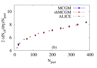
Figure 1: (Color online) Top: The probability distribution of $dN_{ch}/d\eta$ for p+Pb at $\sqrt{s_{\rm NN}}=5.02$ TeV compared between data Chatrchyan et al. , MCGM and shMCGM. Bottom: The centrality dependence of $dN_{ch}/d\eta$ for Pb+Pb at $\sqrt{s_{\rm NN}}=2.76$ TeV compared between data Aamodt et al. (2011), MCGM and shMCGM.

We will now present the results of the shMCGM. In Fig. 1 (a) we have plotted the probability distribution of charged particle multiplicity observed in p+Pb collision at 5.02 TeV for $|\eta|<2.5$ Chatrchyan et al. . We have compared the data with results from both MCGM as well as shMCGM. The nucleons are sampled from a Woods-Saxon distribution of the Pb nuclear density. The Woods-Saxon parameters of the Pb nucleus are: the radius $R=6.7$ fm obtained from the parametrisation $R=1.12A^{0.33}-0.86A^{-0.33}$ and the surface diffusion $\delta=0.54$ fm Kolb and Heinz (2003). We find good description of the long tail in the distribution only after including NBD fluctuation Bozek and Broniowski (2013) with $k\sim 1$. In Fig. 1 (b) we display the centrality dependence of the charged particle multiplicity in Pb+Pb collisions at $\sqrt{s_{\rm NN}}=2.76$ TeV and contrast the results with the available data Aamodt et al. (2011). It is clear that this plot does not discriminate between MCGM and shMCGM as both the models describe the data well for suitably adjusted values of the model parameters. Thus the shadow parameter $\lambda$ can not be fixed from this plot. We have fixed $\lambda$ from the E/E distribution plot of scaled $v_{2}$ assuming linear hydrodynamic response, i.e. $v_{2}\propto\varepsilon_{2}$. The values of the parameters so obtained is tabulated in Table 1. Apart from the parameters listed in Table 1, we need the nucleon-nucleon cross-section $\sigma_{NN}$ which is taken here as $64$ mb (the corresponding value at RHIC is $42$ mb). We take $\sigma=0.5$ fm, which is used in the Gaussian ansatz below to smear the energy $\epsilon_{i}$ deposited by a participant located at $\left(x_{i},y_{i}\right)$,

$$\epsilon_{i}\left(x,y\right) = \frac{\epsilon_{0}}{2\pi\sigma^{2}}e^{-\frac{\left(x-x_{i}\right)^{2}+\left(y-y_{i}\right)^{2}}{2\sigma^{2}}}$$ (6)

Model	$n_{0}$	$f$	$k$	$\lambda$
MCGM	4.05	0.11	1	-
shMCGM	4.05	0.32	1	0.08

Table 1: The values of the parameters of the Glauber models used in this work.

We notice that in both MCGM as well as shMCGM, $n_{0}$ nearly doubles from $\sqrt{s_{\rm NN}}=200$ GeV to $2.76$ TeV. On the other hand, $f$ drops by $20\%$ as we go from RHIC to LHC in MCGM while it stays almost constant in shMCGM. However, the shadow parameter $\lambda$ drops by $25\%$ at LHC compared to highest RHIC energy. This suggests that $\lambda$ increases with decrease in $\sqrt{s_{\rm NN}}$ and hence the distinction between the two Glauber approaches will become even more significant at lower energies (e.g. GSI-FAIR energies).

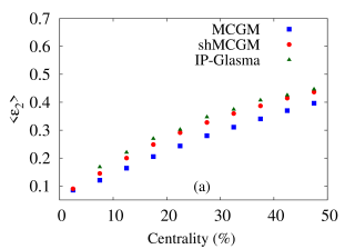
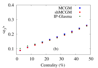
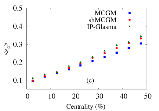
Figure 2: (Color online) The centrality dependence of eccentricities compared between IP-Glasma, MCGM and shMCGM.

Thus, having fixed the parameters of the Glauber models, we now look at the model predictions for other observables and compare them with data as well as results from other dynamical models of IC like IP-Glasma. We first study the centrality dependence of the mean eccentricity harmonics $\varepsilon_{n}$ of the initial energy deposited in the overlap region

$$\varepsilon_{n}e^{i\Psi_{n}} = \frac{\langle r^{n}e^{in\phi}\rangle}{\langle r^{n}\rangle}$$ (7)

where $n=2,3,..$. The coordinate system is chosen such that $\langle\vec{r}\rangle=0$. $\langle...\rangle$ represents averaging over the transverse plane with the initial energy deposited on the transverse plane $\epsilon\left(x,y\right)$ as the weight function. In Fig. 2, we have plotted the ensemble average of $\varepsilon_{2}$, $\varepsilon_{3}$ and $\varepsilon_{4}$ vs their centrality which is determined from the final state (FS) charged hadron multiplicity. We have shown the results for MCGM, shMCGM and IP-Glasma. All the models show a rising trend for $\varepsilon_{2}$ with centrality which is also expected from geometrical arguments- events with lower multiplicity occur with larger impact parameter which results in larger ellipticity of the overlap region. For all centralities, $\varepsilon_{2}$ in shMCGM is enhanced as compared to MCGM and is also in good agreement with IP-Glasma results. The higher value of $\varepsilon_{2}$ in shMCGM as compared to MCGM was also found at RHIC energy and is a typical effect due to nucleon shadowing Chatterjee et al. (2015). The ends of the minor axis of the collision zone have on an average larger number of participants as compared to the ends of the major axis of the overlap region which calls for larger shadowing effect at the ends of the minor axis. This effectively reduces the minor axis more than the major axis, thus increasing the $\varepsilon_{2}$ of the overlap region.

The higher harmonics arise due to granularity in the IC which is controlled by $N_{part}$: smaller $N_{part}$ corresponds to larger granularity Bhalerao et al. (2011); Schenke et al. (2014). This explains the rising trend in $\varepsilon_{3}$ and $\varepsilon_{4}$ with centrality. We note that both MCGM and shMCGM yield almost similar values for these higher eccentricities even though in shMCGM the effective number of participants is smaller than in MCGM due to the shadowing effect. This is so because the shadowing effect systematically weakens only those sources which have other sources in front. Thus, weakening of these sources in the bulk do not increase the granularity in the transverse plane.

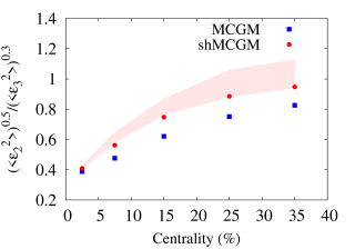
Figure 3: (Color online) The centrality dependence of the ratio of r.m.s. $\varepsilon_{2}$ to $\varepsilon_{3}$ compared between MCGM and shMCGM. Also shown is the band as proposed in Ref. Retinskaya et al. (2014) that is required to explain the correlation of $v_{2}-v_{3}$ in data assuming linear hydrodynamic response.

The correlation between the even-odd harmonics largely stem from the $\varepsilon_{2}-\varepsilon_{3}$ correlation of the initial state (IS). Starting from the observed correlation in the data of $v_{2}-v_{3}$ at the LHC, an allowed band for the ratio of r.m.s values of $\varepsilon_{2}$ to $\varepsilon_{3}$ was obtained in Ref. Retinskaya et al. (2014) within the realm of linear response. In Fig. 3 we have shown this band. We also show the values obtained for the same quantity in MCGM and shMCGM. The enhancement of $\varepsilon_{2}$ in shMCGM as compared to MCGM as noted earlier in Fig. 2 also helps here- it pushes the prediction for the ratio of r.m.s. of $\varepsilon_{2}$ to $\varepsilon_{3}$ into the band that is favored by data unlike the case of MCGM which underpredicts as compared to the band.

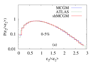
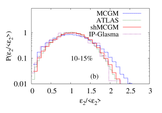
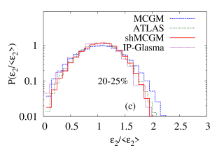
Figure 4: (Color online) The E/E distribution of $\varepsilon_{2}$ compared between data Timmins (2013); Aad et al. (2013), IP-Glasma, MCGM and shMCGM.

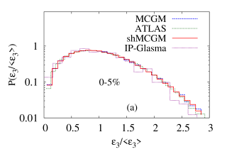
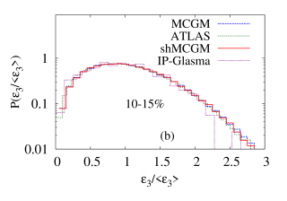
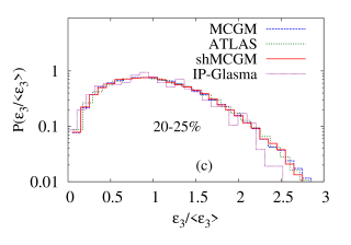
Figure 5: (Color online) The E/E distribution of $\varepsilon_{3}$ compared between data Timmins (2013); Aad et al. (2013), IP-Glasma, MCGM and shMCGM.

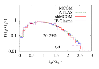
Figure 6: (Color online) The E/E distribution of $\varepsilon_{4}$ compared between data Timmins (2013); Aad et al. (2013), IP-Glasma, MCGM and shMCGM.

We now turn our attention from the mean geometric properties in the IC to their fluctuations. We first analyse the E/E distributions of the $\varepsilon_{n}$ scaled by their ensemble average values and compare with that of IP-Glasma Gale et al. (2013) as well as ATLAS data of $v_{n}$ Timmins (2013); Aad et al. (2013). As long as the hydrodynamic response is linear ($v_{n}=k_{n}\epsilon_{n}$ where $k_{n}$ is a constant), we expect the E/E distributions of $\varepsilon_{n}/\langle\epsilon_{n}\rangle$ to be a good representative of $v_{n}/\langle v_{n}\rangle$. In Figs. 4, 5 and 6 we have plotted the E/E distribution plots for $\varepsilon_{2}$, $\varepsilon_{3}$ and $\varepsilon_{4}$ for the following centrality classes: $\left(0-5\right)\%$, $\left(10-15\right)\%$ and $\left(20-25\right)\%$. Overall, there is good quantitative agreement between shMCGM and data as well as IP-Glasma. It is well known that the standard MCGM produces a broader E/E distribution as compared to data as well as IP-Glasma results Schenke et al. (2014); Niemi et al. (2015). However as already argued earlier in Ref. Chatterjee et al. (2015), the shadowing effect shadows the participants as well as their E/E fluctuations in position which eventually results in narrower E/E distribution that is in good agreement with data and IP-Glasma predictions.

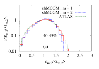
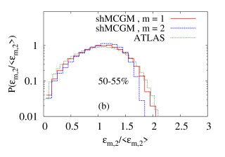
Figure 7: (Color online) The comparison between E/E distribution of $\varepsilon_{1,2}$ and $\varepsilon_{2}$ obtained in shMCGM with data of $v_{2}$ Timmins (2013); Aad et al. (2013).

For further peripheral centralities, the agreement in case of the E/E distributions of $\varepsilon_{2}$ worsen. On the other hand, the distributions of the higher harmonics continue to be in good agreement. Recently, this has been shown as evidence of cubic hydrodynamic response to ellipticity in peripheral collisions Noronha-Hostler et al. (2015). A modified predictor of $v_{2}$, in terms of $\varepsilon_{1,2}$ was shown to do a much better job in the EKRT model for such peripheral bins Niemi et al. (2015) where it is defined as:

$$\varepsilon_{1,2}e^{i\Psi_{1,2}} = \frac{\langle re^{i2\phi}\rangle}{\langle r\rangle}$$ (8)

In Fig. 7 we have plotted the E/E distribution for $\varepsilon_{1,2}$ and compared with the case of $\varepsilon_{2}$ as well as $v_{2}$ from data for the centrality bins of $\left(40-45\right)\%$ and $\left(50-55\right)\%$. We indeed find better agreement between data of $v_{2}$ and shMCGM prediction for $\varepsilon_{1,2}$ than $\varepsilon_{2}$.

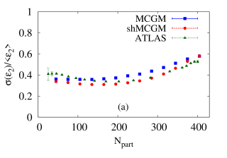
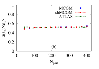
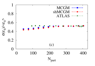
Figure 8: (Color online) The centrality dependence of normalised standard deviation of the eccentricities compared between data Aad et al. (2013), MCGM and shMCGM.

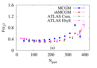
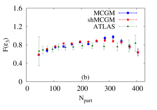
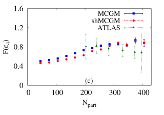
Figure 9: (Color online) The centrality dependence of $F$ of the eccentricities compared between data Aad et al. (2014), MCGM and shMCGM.

The standard deviation is a good measure of fluctuation about the mean value. ATLAS data is available on the scaled variance of the flow coefficients $v_{n}$ which can be compared to that of initial eccentricity assuming linear response Aad et al. (2013). These quantities have been recently shown to agree well with MCGM computations Rybczynski and Broniowski (2015). In Fig. 8, we have plotted the centrality dependence of $\sigma\left(\varepsilon_{n}\right)/\langle\varepsilon_{n}\rangle$ in MCGM and shMCGM. We find almost equally good agreement between data and the different Glauber approaches. Two particle cumulants $\varepsilon_{n}\{2\}$ and four particle cumulants $\varepsilon_{n}\{4\}$ are other quantities of interest that are often measured in experiments and compared to theory,

$$\varepsilon_{n}\{2\} = \langle\varepsilon_{n}^{2}\rangle^{1/2}$$ (9)

$$\varepsilon_{n}\{4\} = \left(2\langle\varepsilon_{n}^{2}\rangle^{2}-\langle\varepsilon_{n}^{4}\rangle\right)^{1/4}$$ (10)

From these cumulants it is possible to define the following scaled moments which within linear response will have one to one correspondence between the initial state(IS) and the final state (FS)

$$F\left(\varepsilon_{n}\right) = \sqrt{\frac{\varepsilon_{n}\{2\}^{2}-\varepsilon_{n}\{4\}^{2}}{\varepsilon_{n}\{2\}^{2}+\varepsilon_{n}\{4\}^{2}}}$$ (11)

We have plotted the centrality dependence of $F\left(\varepsilon_{n}\right)$ in Fig. 9 and find good qualitative agreement between data Aad et al. (2014), MCGM and shMCGM. Thus it is clear from Figs. 3, 4, 8 and 9 that the relative magnitudes of $\varepsilon_{2}-\varepsilon_{3}$ and E/E distribution plots of scaled $\varepsilon_{2}$ can discriminate clearly between MCGM and shMCGM. The rest of the observables have weaker discriminatory power.

IV Summary and Discussions

Glauber models provide a simple and intuitive picture of the initial conditions for the system produced in heavy ion collisions. This model provides the centrality dependence of various ensemble average observables like charged particle multiplicity, anisotropies of the initial energy deposited etc. The MCGM generates event by event distributions of these quantities. The above observables including their event by event distribution can be measured in experiments and compared to such models of initial condition. Overall, Monte-Carlo Glauber models manage to provide a good qualitative description of the data. However, such geometrical models can not describe the recent data on $v_{2}-dN_{ch}/d\eta$ correlation from U+U at $\sqrt{s_{\rm NN}}=193$ GeV and event by event flow data for Pb+Pb at $\sqrt{s_{\rm NN}}=2.76$ TeV. This has called for a lot of ongoing effort to address such issues within the geometric approach of the Glauber model. We have earlier successfully addressed these issues at the top RHIC energy by introducing the effect of shadowing due to leading nucleons on the other participants located in the bulk Chatterjee et al. (2015). Here we have extended our study to Pb+Pb collisions at $\sqrt{s_{\rm NN}}=2.76$ TeV. This idea of eclipse of nucleons in presence of other nucleons inside a nucleus has been proposed about sixty years back Glauber (1955). However, the significance of this effect in the phenomenology of heavy ion collisions has been hardly explored before. The current as well as our earlier work Chatterjee et al. (2015) suggest that the nucleon shadowing plays an important role in the ICs of HICs.

We find that for all centralities $\varepsilon_{2}$ is enhanced while $\varepsilon_{3}$ and $\varepsilon_{4}$ do not change much due to the inclusion of shadowing. This brings the predictions of the shadowed Glauber model for the mean values as well as event by event distributions of the eccentricities in agreement with IP-Glasma results. The relative magnitudes of $\varepsilon_{2}-\varepsilon_{3}$ and event by event distributions of $\varepsilon_{2}$ clearly demonstrate the superior performance of the shadowed Glauber model as compared to its conventional version, MCGM. The shadow parameter $\lambda$ drops by $\sim 25\%$ as we go from top RHIC to LHC energies. This implies that at lower energies, the effect of shadowing in Glauber models will be even more important. Currently for low energies where the fireball is expected to carry a non-zero net baryon number, dynamical models are yet to be formulated and predictions made. On the other hand, within the ambit of the shadowed Monte-Carlo Glauber model, it is straightforward to make predictions at all energies as long as there is a good understanding of the $\sqrt{s_{\rm NN}}$ dependence of the model parameters.

Acknowledgement: We would like to thank Prithwish Tribedy for providing the IP-Glasma data. SC acknowledges him for many fruitful discussions on the initial condition and thanks “Centre for Nuclear Theory” [PIC XII-R$\&$D-VEC-5.02.0500], Variable Energy Cyclotron Centre for support. SG acknowledges Department of Atomic Energy, Govt. of India for support.

References

- Bialas et al. (1976) A. Bialas, M. Bleszynski, and W. Czyz, Nucl. Phys. B111, 461 (1976).
- Eskola et al. (2000) K. J. Eskola, K. Kajantie, P. V. Ruuskanen, and K. Tuominen, Nucl. Phys. B570, 379 (2000).
- Kharzeev and Nardi (2001) D. Kharzeev and M. Nardi, Phys. Lett. B507, 121 (2001).
- Kharzeev et al. (2005) D. Kharzeev, E. Levin, and M. Nardi, Phys. Rev. C71, 054903 (2005).
- Hirano et al. (2006) T. Hirano, U. W. Heinz, D. Kharzeev, R. Lacey, and Y. Nara, Phys. Lett. B636, 299 (2006).
- Miller et al. (2007) M. L. Miller, K. Reygers, S. J. Sanders, and P. Steinberg, Ann. Rev. Nucl. Part. Sci. 57, 205 (2007).
- Broniowski et al. (2009) W. Broniowski, M. Rybczynski, and P. Bozek, Comput. Phys. Commun. 180, 69 (2009).
- Schenke et al. (2012) B. Schenke, P. Tribedy, and R. Venugopalan, Phys. Rev. Lett. 108, 252301 (2012).
- Gale et al. (2013) C. Gale, S. Jeon, B. Schenke, P. Tribedy, and R. Venugopalan, Phys. Rev. Lett. 110, 012302 (2013).
- Rybczynski et al. (2013) M. Rybczynski, W. Broniowski, and G. Stefanek, Phys. Rev. C87, 044908 (2013).
- Goldschmidt et al. (2015) A. Goldschmidt, Z. Qiu, C. Shen, and U. Heinz, Phys. Rev. C92, 044903 (2015).
- Niemi et al. (2015) H. Niemi, K. J. Eskola, and R. Paatelainen, (2015), arXiv:1505.02677 [hep-ph] .
- Woods and Saxon (1954) R. D. Woods and D. S. Saxon, Phys. Rev. 95, 577 (1954).
- Song et al. (2011) H. Song, S. A. Bass, U. Heinz, T. Hirano, and C. Shen, Phys. Rev. Lett. 106, 192301 (2011), [Erratum: Phys. Rev. Lett.109,139904(2012)].
- Adamczyk et al. (2015) L. Adamczyk et al. (STAR), Phys. Rev. Lett. 115, 222301 (2015).
- Moreland et al. (2015) J. S. Moreland, J. E. Bernhard, and S. A. Bass, Phys. Rev. C92, 011901 (2015).
- Chatterjee et al. (2015) S. Chatterjee, S. K. Singh, S. Ghosh, M. Hasanujjaman, J. Alam, and S. Sarkar, (2015), arXiv:1510.01311 [nucl-th] .
- Aamodt et al. (2011) K. Aamodt et al. (ALICE), Phys. Rev. Lett. 106, 032301 (2011).
- Timmins (2013) A. R. Timmins (ALICE), J. Phys. Conf. Ser. 446, 012031 (2013).
- Aad et al. (2013) G. Aad et al. (ATLAS), JHEP 11, 183 (2013).
- Aad et al. (2014) G. Aad et al. (ATLAS), Eur. Phys. J. C74, 3157 (2014).
- Bozek and Broniowski (2013) P. Bozek and W. Broniowski, Phys. Rev. C88, 014903 (2013).
- (23) S. Chatrchyan et al. (CMS), PhysicsResultsHIN12015 .
- Kolb and Heinz (2003) P. F. Kolb and U. W. Heinz, (2003), arXiv:nucl-th/0305084 [nucl-th] .
- Bhalerao et al. (2011) R. S. Bhalerao, M. Luzum, and J.-Y. Ollitrault, Phys. Rev. C84, 054901 (2011).
- Schenke et al. (2014) B. Schenke, P. Tribedy, and R. Venugopalan, Phys. Rev. C89, 064908 (2014).
- Retinskaya et al. (2014) E. Retinskaya, M. Luzum, and J.-Y. Ollitrault, Phys. Rev. C89, 014902 (2014).
- Noronha-Hostler et al. (2015) J. Noronha-Hostler, L. Yan, F. G. Gardim, and J.-Y. Ollitrault, (2015), arXiv:1511.03896 [nucl-th] .
- Rybczynski and Broniowski (2015) M. Rybczynski and W. Broniowski, (2015), arXiv:1510.08242 [nucl-th] .
- Glauber (1955) R. J. Glauber, Phys. Rev. 100, 242 (1955).