Interaction Between Convection and Pulsation

Abstract

This article reviews our current understanding of modelling convection dynamics in stars. Several semi-analytical time-dependent convection models have been proposed for pulsating one-dimensional stellar structures with different formulations for how the convective turbulent velocity field couples with the global stellar oscillations. In this review we put emphasis on two, widely used, time-dependent convection formulations for estimating pulsation properties in one-dimensional stellar models. Applications to pulsating stars are presented with results for oscillation properties, such as the effects of convection dynamics on the oscillation frequencies, or the stability of pulsation modes, in classical pulsators and in stars supporting solar-type oscillations.

1 Introduction

Transport of heat (energy) and momentum by turbulent convection is a phenomenon that we experience on a daily basis, such as the boiling of water in a kettle, the circulation of air inside a non-uniformly heated room, or the formation of cloud patterns. Convection may be defined as fluid (gas) motions brought about by temperature differences with gradients in any direction (Koschmieder, 1993). It is not only important to engineering applications but also to a wide range of astrophysical flows, such as in galaxy-cluster plasmas, interstellar medium, accretion disks, supernovae, and during several evolutionary stages of all stars in the Universe. The transport of turbulent fluxes by convection is mutually affected by other physical processes, including radiation, rotation, and any kind of mixing processes. In stars turbulent convection affects not only their structure and evolution but also any dynamical processes with characteristic time scales that are similar to the characteristic time scale of convection in the overturning stellar layers. One such important process is stellar pulsation, the study of which has become the field of asteroseismology. Asteroseismology and, when applied to the Sun, helioseismology, is now one of the most important diagnostic tools for testing and improving the theory of stellar structure and evolution by analysing the observed pulsation properties. It is, therefore, the aim of this review to provide an up-to-date account on the most widely used stellar convection models with emphasis on the formalisms that describe the interaction of the turbulent velocity field with the stellar pulsation.

The temperature in a star is determined by the balance of energy and its gradient depends on the details how energy is transported throughout the stellar interior. Red giants and solar-like stars exhibit substantial convection zones in the outer stellar layers, which affect the properties of the oscillation modes such as the oscillation frequencies and mode stability. Among the first problems of this nature was the modelling of the red edge of the classical instability strip in the Hertzsprung–Russell diagram which, for intermediate-mass stars with about $1.5\mbox{\,--\,}2.0\,M_{\odot}$, is located approximately at surface temperatures between 7200 – 6600 K. The first pulsation calculations of classical pulsators without any pulsation-convection modelling predicted red edges which were much too cool and which were at best only neutrally stable. What followed, were several attempts to bring the theoretically predicted location of the red edge in better agreement with the observed location by using time-dependent convection models in the pulsation analyses (e.g., Deupree, 1977b; Baker and Gough, 1979; Gonczi, 1982b; Stellingwerf, 1984). Later, several authors, e.g., Bono et al. (1995, 1999), Houdek (1997, 2000), Xiong and Deng (2001, 2007), Dupret et al. (2005a, b) were successful to model the red edge of the classical instability strip, and mode lifetimes in stars supporting solar-like oscillations (e.g., Gough, 1980; Balmforth, 1992a; Houdek et al., 1999a; Xiong et al., 2000; Houdek and Gough, 2002; Dupret et al., 2004a; Chaplin et al., 2005; Dupret et al., 2006a; Houdek, 2006; Dupret et al., 2009; Belkacem et al., 2012).

Thermal heat transport in convective regions is governed by turbulent motion of the underlying fluid or gas. To determine the average of vertical velocity, temperature and momentum fluctuations, the full structure of the turbulent flow is needed. This is until today not a tractable theoretical problem without the introduction of some hypothetical assumptions in order to close the system of equations describing the turbulent flow. Such closure models can be classified basically into four categories: (i) ‘algebraic models’, including the mixing-length approach (e.g., Prandtl, 1925; Vitense, 1953; Böhm-Vitense, 1958), (ii) ‘one-equation models’, which use a modified turbulent kinetic energy equation with high-order moments closed approximately by means of a locally defined mixing length (e.g., Rodi, 1976; Stellingwerf, 1982), (iii) ‘two-equation models’, such as the $K-\epsilon_{\mathrm{t}}$ model, where $K$ denotes the turbulent kinetic energy and $\epsilon_{\mathrm{t}}$ the associated viscous dissipation of turbulent energy (e.g., Jones and Launder, 1972, 1973), and (iv) ‘Reynolds stress models’, which use transport equations for all second-order moments (typically five) including the turbulent fluxes of heat and momentum, and appropriate approximation for the third-order moments to close the equations (e.g., Keller and Friedmann, 1924; Rotta, 1951; Castor, 1968; Xiong, 1977; Canuto, 1992; Grossman, 1996; Canuto and Dubovikov, 1998; Kupka, 1999; Montgomery and Kupka, 2004; Xiong and Deng, 2007).

Theories based on the mixing-length formalism (Prandtl, 1925) still represent the main method for computing the stratification of convection zones in stellar models. An alternative convection formulation, based on the Eddy-Damped Quasi-Normal Markovian approximation to turbulence (e.g., Orszag, 1977), was introduced by Canuto and Mazzitelli (1991) which, however, still requires a (local) mixing length for estimating the convective heat (enthalpy) flux. The Eddy-Damped Quasi-Normal Markovian approximation is characterized as a two-equation model and is sometimes referred to as two-point closure, because it describes correlations of two different points in space, or two different wave numbers $\bm{k}$ and $\bm{k^{\prime}}$ in Fourier space. Although two-equation models have a reasonable degree of flexibility, they are restricted by the assumption of a scalar turbulent viscosity and that the stresses are proportional to the rate of mean strain. The Reynolds stress models are, in principle, free of these restrictions and were discussed, for example, by Xiong (1989) and Canuto (1992, 1993) for the application in stellar convection. Xiong’s model was applied successfully to various types of pulsating star, and Canuto’s model was applied to non-pulsating stars with relatively shallow surface convection zones (Kupka and Montgomery, 2002; Montgomery and Kupka, 2004).

Time-dependent convection models are required to describe the interaction between the turbulent velocity field and the oscillating stellar background. Semi-analytical models for pulsating stars were proposed, for example, by Schatzman (1956), Gough (1977a), Unno (1967), Xiong (1977), Stellingwerf (1982), Gonczi (1982a), Kuhfuß (1986), and Grossman (1996).

The present unprecedented computer revolution enables us to perform fully hydrodynamical simulations of large-scale turbulent flows (large eddy simulation) of stellar surface convection (e.g., Stein and Nordlund, 1989, 2000; Nordlund et al., 1996; Trampedach et al., 1998; Kim et al., 1996; Chan and Sofia, 1996; Freytag et al., 2002; Robinson et al., 2004; Wedemeyer et al., 2004; Muthsam et al., 2010; Magic et al., 2013; Trampedach et al., 2013, 2014a; Magic et al., 2015). A review of three-dimensional (3D) hydrodynamical simulations of the Sun, together with their shortcomings, was presented by Miesch (2005). Such numerical simulations represent a fruitful tool for investigating the accuracy and hence the field of application of phenomenological prescriptions of convection such as the mixing-length approach.

In this review, we summarize the two time-dependent convection models by Gough (1965, 1977a) and Unno (1967, 1977) for estimating stellar stability properties in classical pulsators and solar-type stars. In Section 2, we start from the equations of fluid motion to derive first the mean and fluctuating equations within the commonly adopted Reynolds separation approach. Section 3 discusses first the time-dependent convection equations by Gough (1965, 1977a) and Unno (1967, 1977) for radially pulsating stellar envelopes, followed by a summary of Gough77b nonlocal equations, before embarking on a discussion on a generalization of Unno67 model to nonradial stellar oscillations by Gabriel et al. (1975) and Grigahcène et al. (2005). A summary of Reynolds stress models adopted to stellar convection is provided in Section 4. Applications of the two time-dependent convection models by Gough (1977a, b) and Grigahcène et al. (2005) are provided in Sections 5, 6, and 7, starting with the role of convection dynamics on the oscillation frequencies, the so-called surface effects, followed by a summary of our current understanding of mode physics in classical pulsators and stars supporting solar-like oscillations. Final remarks and prospects are given in Section 8.

2 Hydrodynamical Equations

For simplicity we neglect any symmetry-breaking agents such as rotation or magnetic fields and adopt spherical geometry for which, for example, the velocity field $\bm{u}=(u_{\mathrm{r}},u_{\varphi},u_{\theta})$. In this approximation the fluid conservation equations for mass, momentum and thermal energy equation, using vector notation, are (Ledoux and Walraven, 1958; Landau and Lifshitz, 1959; Batchelor, 1967)

$$\frac{\partial\rho}{\partial t}+\nabla\cdot\left(\rho\bm{v}\right)=0\,,$$ (1)

$$\frac{\partial\left(\rho\bm{v}\right)}{\partial t}+\nabla\cdot\left(\rho\bm{vv}\right)=\rho\bm{g}+\nabla\cdot\bm{\uptau}\,,$$ (2)

$$\frac{\partial(\rho e)}{\partial t}+\nabla\cdot\left(\rho e\bm{v}\right)-\bm{\uptau}{\,:\,}\nabla\bm{v}=\rho\varepsilon-\nabla\cdot\bm{F}_{\mathrm{R}}\,,$$ (3)

where $\rho$ is density, $\bm{v}$ the velocity vector, $\bm{g}=(-g,0,0)$ with $g$ being the magnitude of the gravitational acceleration, $\bm{\uptau}:=-p\,\mathbf{I}\,+\,\bm{\upsigma}$, with $p$ being the sum of the gas and radiative pressures ($\mathbf{I}$ is the unity or identity matrix), and $\bm{\upsigma}$ is the sum of the gaseous and radiative deviatoric (viscous) stress tensors; $e$ is the specific internal energy, $\varepsilon$ is the rate of energy generation per unit mass by nuclear reactions and $\bm{F}_{\mathrm{R}}$ is the radiative flux. The dissipation of energy by internal stress and (reversible) interchange with strain energy is indicated by $\bm{\uptau}\,:\,\nabla\bm{v}=-p\,\nabla\cdot\bm{v}+\bm{\upsigma}:\nabla\bm{v}$, which is the dyadic notation for $\uptau_{ij}v_{i,j}$.

2.1 Mean equations

We follow the standard Reynolds approach and separate all variables into an average (or mean) part, and into a fluctuating part. Thus

$$y=\overline{y}+y^{\prime},$$ (4)

$$\bm{v}=\bm{U}+\bm{u},$$ (5)

where $y$ is any of the variables $\rho$, $p$, $T$, etc., and $\overline{y}$ and $\bm{U}$ are the appropriately averaged mean values (i.e., typically horizontal averages). The fields $y^{\prime}$ and $\bm{u}$ are convective (Eulerian) fluctuations. The separation of the velocity into mean and fluctuating components must be carried out with some care. Because there is no mean transport of mass (mass flux) across layers with constant radius, we adopt (e.g., Ledoux and Walraven, 1958; Unno, 1967; Gough, 1969; Gabriel et al., 1975; Gough, 1977a; Unno and Xiong, 1990; Grigahcène et al., 2005)

$$\overline{\rho\bm{u}}=0\,,\quad\overline{\bm{u}}\neq 0\,.$$ (6)

We further define the time derivative following the pulsational motion by (e.g., Ledoux and Walraven, 1958; Unno, 1967; Gough, 1969, see also Section 2.2)

$$\frac{\,\mathrm{d}missing}{\,\mathrm{d}t}=\frac{\partial}{\partial t}+\bm{U}\cdot\nabla.$$ (7)

The mean equations of mass and momentum conservation are obtained from taking averages of the Eqs. (1) and (2). Stellar turbulence is characterized by high Reynolds numbers $R_{\mathrm{e}}$, typically in the order of $R_{\mathrm{e}}\geq 10^{12}$. We, therefore, can neglect the viscous stress tensor $\overline{\bm{\upsigma}}$ in the momentum equation (2) and obtain for the averaged continuity and momentum equations

$$\frac{\partial\overline{\rho}}{\partial t}+\nabla\cdot\left(\overline{\rho}\bm{U}\right)=0,$$ (8)

$$\overline{\rho}\frac{\,\mathrm{d}\bm{U}}{\,\mathrm{d}t}=\overline{\rho}\,\overline{\bm{g}}-\nabla(\overline{p}+p_{\mathrm{t}})-\nabla\cdot\bm{\upsigma}_{\mathrm{t}}\,,$$ (9)

in which we neglected the perturbation to the gravitational acceleration. In the literature (e.g., Ledoux and Walraven, 1958; Unno and Xiong, 1990) it is common to adopt Boussinesq’s suggestion for representing the turbulent stresses in a similar way as for the viscous stresses, i.e., to separate the Reynolds stress tensor $\overline{\rho\,\bm{uu}}$ into an isotropic component $\hat{p}_{\mathrm{t}}$, which is typically called the turbulent pressure, and into a nonisotropic (deviatoric) part $\bm{\upsigma}_{\mathrm{t}}$,

$$\overline{\rho\bm{uu}}:=\tilde{p}_{\mathrm{t}}\,{\mathbf{I}}+{\bm{\upsigma}_{\mathrm{t}}}\,.$$ (10)

Here $\tilde{p}_{\mathrm{t}}:=\overline{\rho|\bm{u}|^{2}}/3$, and $\sigma_{ij,\mathrm{t}}:=\mu_{\mathrm{t}}[(2/3)\partial_{k}\overline{v_{k}}\delta_{ij}-\partial_{i}\overline{v_{j}}-\partial_{j}\overline{v_{i}}]$, where $\delta_{ij}$ is the Kronecker delta, and $\mu_{\mathrm{t}}$ represents a scalar turbulent (eddy) viscosity. Equation (10) is, however, strictly valid only for isotropic turbulence but the convective velocity field in stars is, in general, predominantly anisotropic (e.g., Houdek, 2012). In this review we shall therefore follow Gough (1977a) and parametrize the anisotropy of the turbulent velocity field $\bm{u}=(u_{\mathrm{r}},u_{\theta},u_{\phi})$ by the anisotropy parameter

$$\overline{\Phi}:=\frac{\overline{\rho|\bm{u}|^{2}}}{\overline{\rho u_{\mathrm{r}}^{2}}}\,,$$ (11)

and define the turbulent pressure

$$p_{\mathrm{t}}:=\overline{\rho{u_{\mathrm{r}}u_{\mathrm{r}}}}$$ (12)

as the $(r,r)-$component of the Reynolds stress tensor $\overline{\rho\bm{uu}}$. Note that $\Phi=3$ represents an isotropic velocity field.

The mean equation for the turbulent kinetic energy is obtained by multiplying Eq. (2) by $\bm{v}$ and Eq. (9) by $\bm{u}$, followed by averaging the difference between the resulting expressions. The outcome is

$$\overline{\rho}\frac{\,\mathrm{d}missing}{\,\mathrm{d}t}\left(\frac{1}{2}\frac{\overline{\rho\bm{u}^{2}}}{\overline{\rho}}\right) = -\overline{\rho\bm{uu}}:\nabla\bm{U}-\overline{\bm{u}\cdot\nabla p}-\frac{1}{2}\nabla\cdot\left(\overline{\rho\bm{u}^{2}\bm{u}}\right)-\overline{\bm{\upsigma}:\nabla\bm{u}}+\nabla\cdot\overline{\left(\bm{\upsigma}\cdot\bm{u}\right)}\,,$$ (13)

where the last term on the right-hand side is small and can therefore be neglected (e.g., Ledoux and Walraven, 1958). The first two terms on the right-hand side represent respectively the production of turbulent kinetic energy from the mean motion and from the gravitational potential energy. The third term on the right-hand side is the divergence of the turbulent kinetic energy flux and the fourth term is the dissipation of kinetic energy (per unit volume) into heat. We emphasize here a significant difference with other studies. In this review we adopt Eq. (6) for the averaging process, which leads to no buoyancy term in Eq. (13). If, however, instead $\overline{\bm{u}}=0$ is assumed, the additional buoyancy term, $\overline{\rho^{\prime}\bm{u}\cdot\bm{g}}$, appears on the right-hand side of the kinetic energy equation (e.g., Canuto, 1992), where $\bm{g}$ is the gravitational acceleration.

The mean equation of the thermal energy conservation is obtained by taking the average of Eq. (3):

$$\overline{\rho}\frac{\mathrm{d\,\overline{e}}}{\,\mathrm{d}t}+\overline{p}\,\nabla\cdot\bm{U}=\overline{\rho\varepsilon}-\nabla\cdot\left(\overline{\bm{F_{\mathrm{r}}}}+\overline{\rho{h}\bm{u}}\right)+{\overline{\bm{u}\cdot\nabla p}}+\overline{\bm{\upsigma}:\nabla\bm{u}}\,,$$ (14)

where $h=e+p/\rho$ is the (specific) enthalpy. Essentially, all semi-analytical stellar convection models adopt the Boussinesq approximation to the equations of motion (Spiegel and Veronis, 1960). This approximation is valid for fluids for which the vertical dimension of the fluid is much less than any scale height, and the motion-induced density and pressure fluctuations must not exceed, in order of magnitude, the mean values of these quantities, i.e., the Mach number of the fluid, which is the ratio of the fluid velocity over the adiabatic sound speed, must remain small. Part of the Boussinesq approximation is to neglect squares of fluctuating thermodynamic quantities, and neglecting pressure fluctuations $p^{\prime}$ compared to $\rho^{\prime}$ or $e^{\prime}$ (see also Section 3.2). These conditions are believed not to be satisfied everywhere in stars, in particular in the superadiabatic boundary layer, yet we shall adopt it here in this review. Within the Boussinesq approximation the mean equations for the conservation of mass and momentum are identical to Eqs. (8) and (9) respectively. The mean equations for the conservation of turbulent kinetic energy (13), thermal energy (14) and anisotropy of the turbulent velocity field (11) become:

$$\frac{\overline{\rho}}{2}\frac{\mathrm{d\,\overline{|\bm{u}|^{2}}}}{\,\mathrm{d}t} = -\overline{\rho\bm{uu}}{\,:\,}\nabla\bm{U}-\overline{\bm{u}}\cdot\nabla\overline{p}-\overline{\rho}\epsilon_{\mathrm{t}}\,,$$ (15)

$$\overline{\rho}\,\overline{T}\,\frac{\mathrm{d}\overline{s}}{\,\mathrm{d}t}=\overline{\rho}\,\overline{\varepsilon}-\nabla\cdot\left(\overline{\bm{F}}_{\mathrm{R}}+\bm{F}_{\mathrm{c}}\right)+\overline{\bm{u}}\cdot\nabla\overline{p}+\overline{\rho}\,{\epsilon_{\mathrm{t}}}\,,$$ (16)

$$\overline{\Phi}:=\frac{\overline{|\bm{u}|^{2}}}{\overline{u_{\mathrm{r}}^{2}}}\,,$$ (17)

where the vector field ${\bm{F}}_{\mathrm{c}}$ is the convective heat (enthalpy $h$) flux

$${\bm{F}}_{\mathrm{c}}:=\overline{\left(p+\rho e\right)^{\prime}\bm{u}}=\overline{\rho h^{\prime}\bm{u}},$$ (18)

which can be further simplified within the Boussinesq approximation to

$$\bm{F}_{\mathrm{c}}\simeq\overline{\rho}\,\overline{T}\>\overline{\bm{u}s^{\prime}}=\overline{\rho}\,\overline{c_{\mathrm{p}}}\overline{\bm{u}T^{\prime}}\,,$$ (19)

($s$ is specific entropy, $T$ is temperature, and $c_{\mathrm{p}}$ the specific heat at constant pressure), and $\overline{\rho}\epsilon_{\mathrm{t}}=\overline{\bm{\upsigma}:\nabla\bm{u}}$ is the viscous dissipation of turbulent kinetic energy (per unit volume) into heat (sink term in the kinetic energy equation). For an incompressible Newtonian fluid the viscous dissipation of turbulent kinetic energy $\overline{\rho}\epsilon_{\mathrm{t}}=2\mu\overline{e_{ij}e_{ij}}$, where $e_{ij}:=(\partial_{j}u_{i}+\partial_{i}u_{j})/2$ is the fluctuating strain rate and $\mu$ is the (constant) molecular (dynamic) viscosity. The penultimate term on the right-hand side of the turbulent kinetic energy equation (15) is the work of the pressure gradient transforming gravitational potential energy into kinetic energy of turbulence (source term). Both terms $-\overline{\bm{u}}\cdot\nabla\overline{p}-\overline{\rho}\epsilon_{\mathrm{t}}$ are also present with opposite sign in the mean thermal energy equation (16). For the stationary ($\partial/\partial t=0$) equilibrium state with no mean flow ($\bm{U}=\bm{0}$) the turbulent kinetic energy is constant. Consequently these two terms vanish and are therefore neglected in the mean thermal energy equation (16) in the Boussinesq approximation (see also Spiegel and Veronis, 1960). We shall, however, see later that its perturbation due to oscillations may not necessarily vanish, even at second order. The turbulent kinetic-energy flux [third term on the right-hand side of Eq. (13)] is not necessarily small everywhere. According to three-dimensional hydrodynamical simulations of the outer atmospheric layers in the Sun, the kinetic energy flux can be as large as $\sim$ 15% of the total energy flux (e.g., Trampedach et al., 2014a), yet it is typically ignored in semi-analytical convection models. We follow the same approximation and omit this term in Eq. (15). An expression for the kinetic energy flux within the mixing-length approach was recently provided by Gough (2012a).

2.2 Boussinesq mean equations for radially pulsating atmospheres

One of the first questions to ask is how one would go about the separation of the velocity field into a component that is associated with the stellar pulsation and into another component that is related to the convection. The answer is not necessarily straightforward (for a recent discussion see, e.g., Appourchaux et al., 2010, $\mathsection$3.1). This separation of the velocity field is probably best known for radial pulsations, for which the horizontal motion is uniform (the convective motion is not). By adopting Eq. (6) for averaging the horizontal motion of the convective velocity field the radial pulsations can be separated in an (mathematically) obvious way (e.g., Gough, 1969), in which the small-scale convective Eulerian fluctuations ($\bm{u}$) are advected by the large-scale radial Lagrangian motion ($U$) of the pulsation.

Below, we follow the discussion by Gough (1977a) and summarize the mean Boussinesq equations for radial pulsations adopting a mixed Lagrangian-Eulerian coordinate system ($q_{i}$) defined in terms of spherical polar coordinates $(r,\theta,\varphi)$

$$(\,\mathrm{d}q_{1},\,\mathrm{d}q_{2},\,\mathrm{d}q_{3})=(r\,\mathrm{d}\theta,r\sin\theta\,\mathrm{d}\varphi,{\overline{\rho}}\,\mathrm{d}r)\,,$$ (20)

where $q_{3}=0$ at $r=0$, and an overbar means, as before, an instantaneous average over a spherical surface with constant $r$ (i.e., horizontal average). As already mentioned before, the introduction of Eq. (6) in this coordinate system has the property that there is no mean mass flux across a surface with $q_{3}=\,$constant (Ledoux and Walraven, 1958; Gough, 1969, 1977a) and this coordinate system describes the large-scale pulsational motion of a fluid layer in a Lagrangian frame of reference, whereas inside this moving layer the convective motion is described in an Eulerian frame. The time derivative at constant (Eulerian) $q_{i}$ is then related to that in spherical polar coordinates by [see also Eq. (7)]

$$\left(\frac{\partial}{\partial t}\right)_{q_{i}}=\left(\frac{\partial}{\partial t}\right)_{r,\theta,\phi}+\,\overline{\rho}\,U\,\frac{\partial}{\partial q_{3}}\,,$$ (21)

where $U=(\partial r/\partial t)_{q_{3}}$. Within this adopted coordinate system, the mean equations for the radial component of the momentum equation and the thermal energy equation in the Boussinesq approximation become with $\varepsilon=0$ and $q=q_{3}$ (Gough, 1977a):

$$\frac{\partial}{\partial q}({\overline{p}}+p_{\mathrm{t}})+(3-{\overline{\Phi}})\frac{p_{\mathrm{t}}}{r{\overline{\rho}}}=-\frac{{\mathrm{G}}m}{r^{2}}-\frac{\partial^{2}r}{\partial t^{2}}\,,$$ (22)

$$\overline{c_{\mathrm{p}}}\frac{\partial\overline{T}}{\partial t}-\frac{\overline{\hat{\delta}}}{\overline{\rho}}\frac{\partial\overline{p}}{\partial t}=-\frac{1}{r^{2}}\frac{\partial}{\partial q}\left[r^{2}\left(\overline{F_{3}}+F_{\mathrm{c}}\right)\right]\,,$$ (23)

$$\frac{1}{r^{2}}\frac{\partial}{\partial q}\left(r^{2}\overline{F_{3}}\right)=4\pi\overline{\varkappa}\left(\overline{B}-\overline{J}\right)\,,$$ (24)

$$\frac{\partial\overline{J}}{\partial q}=-\frac{3}{4\pi}\overline{\varkappa}\overline{F_{3}}\,,$$ (25)

where

$$\overline{\Phi}=\frac{\overline{u_{i}u_{i}}}{\overline{w^{2}}}\,,$$ (26)

$$p_{\mathrm{t}}:=\overline{\rho u_{3}u_{3}}\simeq\overline{\rho}\,\overline{ww}\,,\$$ (27)

and

$$F_{\mathrm{c}}:=\overline{\rho u_{3}h^{\prime}}\simeq\overline{\rho}\,\overline{c_{\mathrm{p}}}\,\overline{wT^{\prime}}\,,$$ (28)

are respectively the anisotropy parameter [see also Eq. (17)], the $(r,r)$-component of the Reynolds stress tensor $\overline{\rho u_{i}u_{j}}\,$, with $u_{i}=(u,v,w)$, and the convective heat flux in the Boussinesq approximation; $\hat{\delta}:=-(\partial\ln\rho/\partial\ln T)_{p}$ is the isobaric expansion coefficient, and $\varkappa$ is the Rosseland mean opacity.

The second term on the left-hand side of Eq. (22) results from taking the horizontal average of the radial component of the nonlinear advection term $\rho\bm{v}\cdot\nabla\bm{v}$: with the definition of the Reynolds stress tensor (10) and velocity anisotropy (26) the last term of Eq. (9), $(\nabla\cdot\bm{\sigma}_{\mathrm{t}})_{\mathrm{r}}=(3-\overline{\Phi})p_{\mathrm{t}}/r$, assuming axisymmetric turbulence about the radial direction. From a physical point of view this term arises because horizontal motion, in spherical coordinates, transfers momentum in the radial direction, resulting from a difference in the net radial force between the horizontal component of $\overline{\rho u_{i}u_{j}}\,$ for $\overline{\Phi}\neq 3$, and the radial component of magnitude $p_{\mathrm{t}}$ for $\overline{\Phi}=3$ (Gough, 1977a).

The radiative flux $\overline{\bm{F}}=(0,0,\overline{F_{3}})$ is typically treated in the diffusion approximation to radiative transfer. Here we adopt the general, grey Eddington approximation by Unno and Spiegel (1966), given by Eqs. (24) and (25), where $B$ is the Planck function, $J$ is the mean intensity, and $\varkappa$ is the Rosseland-mean opacity. Note that in Eq. (25) one should actually use the Planck-mean opacity, which is the more appropriate mean for optically thin layers (e.g., Mihalas, 1978), instead of the Rosseland-mean opacity. In radiative equilibrium the radiative flux has zero divergence and consequently $\overline{J}=\overline{B}$, reducing the Eddington approximation (24) – (25) to the diffusion approximation

$$\overline{F_{3}}=-\frac{4ac\overline{T}^{3}}{3\overline{\varkappa}}\frac{\partial\overline{T}}{\partial q}\,,$$ (29)

where $a$ is the radiation density constant and $c$ is the speed of light.

The mean equations for a Boussinesq fluid in a radially pulsating star are Eqs. (22)-(28), supplemented by the continuity equation

$$\frac{\,\mathrm{d}m}{\,\mathrm{d}q}=4\pi r^{2}\,.$$ (30)

Note that mass $m$ is a Lagrangian coordinate (i.e., independent of time) in a radially moving atmosphere.

In the mean equations, the turbulent pressure (Reynolds stress) $p_{\mathrm{t}}$ and convective heat flux $F_{\mathrm{c}}$ are the quantities that must be determined from the equations for the convective fluctuations. To solve these equations, a model for the convective turbulence is required, which is discussed in the next section.

3 Time-dependent Mixing-Length Models

3.1 Introduction

The simplest closure model of turbulence is the early one by Boussinesq (1877), who suggested that turbulent flow could be considered as having an enhanced viscosity, a turbulent (or eddy) viscosity $\nu_{\mathrm{t}}$. Boussinesq assumed $\nu_{\mathrm{t}}$ to be constant, in which case the equations of mean motion become identical in structure with those for a laminar flow. This assumption, however, does become invalid near the convective boundary layers, where the turbulent fluctuations vanish, and so does $\nu_{\mathrm{t}}$, at least in a local convection model.

The simplest turbulence model able to account for the variability of the turbulent mixing with the use of only one empirical constant is the mixing-length idea, introduced independently by Taylor (1915) and Prandtl (1925). Based on Boussinesq’s approach and considering the turbulent fluid decomposed into so-called eddies, parcels or elements, Prandtl obtained, for the case of shear flow, from dimensional reasoning, an expression for the turbulent viscosity or exchange coefficient of momentum (“Austauschkoeffizient”). This expression is in the form of a product of the velocity fluctuation perpendicular (transverse) to the mean motion of the turbulent flow and the mixing length $\ell$. The mixing length is characterized by the distance in the transverse direction which must be covered by a fluid parcel travelling with its original mean velocity in order to make the difference between its velocity and the velocity in the new layer equal to the mean transverse fluctuation in the turbulent flow. Inherent in this physical picture is the major assumption that the momentum of the turbulent parcel is assumed to be constant along the travel distance $\ell$, which is analogous to neglecting the streamwise pressure forces and viscous stresses. Prandtl’s concept of a mixing length may be compared, up to a certain point, with the mean free path in the kinetic theory of gases. A somewhat different result was obtained by Taylor (1932) who assumed that the rotation (vorticity) during the transverse motion of the parcel remains constant, yielding a mixing length which is larger by a factor $\sqrt{2}$ compared with Prandtl’s momentum-transfer picture.

Neglecting rotation and magnetic fields, thermal heat transport in stars corresponds to the case of free convection where there is no externally imposed velocity scale as in shear flow. Hence, it is necessary to consider the dynamics of the turbulent elements in greater detail. The imbalance between buoyancy forces, pressure gradients and nonlinear advection processes causes the turbulent elements to accelerate during their existence. Ignoring different combinations of these processes and approximating the remaining terms in different ways, various phenomenological models can be established. In the astrophysical community basically two physical pictures have emerged, which were first applied to stellar convection by Biermann (1932, 1938, 1943, 1948) and Siedentopf (1933, 1935). In both physical pictures the turbulent element is considered as a convective cell with a characteristic vertical length $\ell$ as illustrated in Figure 1.

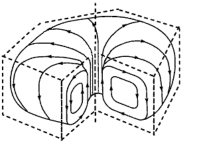
Figure 1: Sketch of an overturning hexagonal (dashed lines) convective cell with vertical extent $\ell$. Near the centre the gas raises from the hot bottom to the cooler top (surface) where it moves nearly horizontally towards the edges, thereby loosing heat. The cooled gas then descends along the edges to close the circular flow. Arrows indicate the direction of the flow pattern. Image adapted from Swenson (1997).

The first physical picture interprets the turbulent flow by direct analogy with kinetic gas theory. The motion is not steady and one imagines the overturning convective element to accelerate from rest followed by an instantaneous breakup after the element’s lifetime. Thus the nonlinear advection terms are neglected in the convective fluctuation equations but are taken to be responsible for the creation and destruction of the convective eddies (Spiegel, 1963; Gough, 1977a, b). By retaining only the acceleration terms the equations become linear and the evolution of the fluid properties carried by the turbulent parcels can be approximated by linear growth rates. The mixing length $\ell$ enters in the calculation of the eddy’s survival probability for determining the convective heat and momentum fluxes (see Appendix A).

In the second physical picture the fluid element maintains exact balance between buoyancy force and turbulent drag by continuous exchange of momentum with other elements and its surrounding (Prandtl, 1932). Thus the acceleration terms are unimportant in a static atmosphere and the evolution of the convective fluctuations are independent of the initial conditions. The nonlinear advection terms (i.e., momentum exchange) provide dissipation (of kinetic energy) that balances the driving terms, and are approximated appropriately (e.g., Kraichnan, 1962; Unno, 1967), leading to two nonlinear equations which need to be solved numerically together with the mean equations of the stellar structure.

The two physical pictures are complementary in envelopes that do not pulsate (Gough, 1977a). However, in a time-dependent formulation additional information is required how the initial state of a convective element depends on conditions at the time of its creation. Hence, the different versions of mixing-length models yield different formulae for the turbulent heat and momentum fluxes when applied to pulsating stars (Unno, 1967; Gough, 1977a, 2012a).

In the above discussed models, the overturning fluid parcels were still considered to move adiabatically. Öpik (1950) suggested to treat radiative heat exchange between the element and the background fluid in a similar way as for the momentum exchange. Based on this assumptions Vitense (1953) and Böhm-Vitense (1958) established a mixing-length description which is still widely used for calculating the convective heat flux in stellar models.

The perhaps simplest description to model the temporal modulation of the convection by the oscillations, put forward in the 1960s, is to presume that the convective fluxes simply relax exponentially on a timescale $\tau_{\mathrm{c}}$ towards the time-independent formula $\,\mathrm{d}F_{\mathrm{c}}/\,\mathrm{d}t=(F_{\mathrm{c0}}-F_{\mathrm{c}})/\tau_{\mathrm{c}}$, where $F_{\mathrm{c}}$ is a component of any turbulent flux and $F_{\mathrm{c0}}$ is the formula for $F_{\mathrm{c}}$ in a statistically steady environment. The constant $\tau_{\mathrm{c}}$ is a multiple of $w/\ell$ with $\ell$ being the mixing length and $w$ a characteristic convective velocity.
In the past, various time-dependent convection models were proposed, for example, by Schatzman (1956), Gough (1965, 1977a), Unno (1967, 1977), Xiong (1977, 1989), Stellingwerf (1982), Gonczi (1982a), Kuhfuß (1986), Unno et al. (1989), Canuto (1992), Gabriel (1996), Grossman (1996), and Grigahcène et al. (2005). Here, we shall review and compare the basic concepts of two, currently in use, convection models. The first model is that by Gough (1977a, b), which has been used, for example, by Baker and Gough (1979), Balmforth (1992a), Houdek et al. (1995), Rosenthal et al. (1995), Houdek (1997, 2000), Houdek et al. (1999a), and Chaplin et al. (2005). The second model is that by Unno (1967, 1977), upon which the generalized models by Gabriel (1996) and Grigahcène et al. (2005) are based, with applications by Dupret et al. (2005c, a, b, 2006a, 2006b, 2006c, 2009), Belkacem et al. (2008, 2009, 2012), and Grosjean et al. (2014).

3.2 Two time-dependent convection models for radially pulsating stars

Unno (1967) and Gough (1965, 1977a) generalized the mixing-length formulation for modelling the interaction of the turbulent velocity field with radial pulsation. Both authors adopted the Boussinesq approximation. The mean equation of motions were already discussed in Section 2.2 for a radially pulsating atmosphere. Therefore, we start here with the Boussinesq approximation for the convective fluctuations. This approximation is based on a careful scaling argument and an expansion in small parameters, i.e., the ratio of the maximum density variation across the layer over the (constant) spatial density average, and the ratio of the fluid layer height to the locally defined smallest scale height (Spiegel and Veronis, 1960; Mihaljan, 1962; Gough, 1969).

In this subsection we follow the discussion by Gough (1977a).

3.2.1 Boussinesq fluctuation equations

The Boussinesq approximation results in (i) an incompressible fluid, which renders the convective velocity field $\bm{u}$ in the continuity equation to be divergence-free, i.e., $\nabla\cdot\bm{u}=0$, (ii) neglecting the density fluctuations $\rho^{\prime}$ in the momentum equation, except when they are coupled to the gravitational acceleration in the (driving) buoyancy force, (iii) neglecting squares of fluctuating thermodynamic quantities, such as $\rho^{\prime}T^{\prime}$, where $T^{\prime}$ is the temperature fluctuation, and neglecting pressure fluctuations $p^{\prime}$ compared to $\rho^{\prime}$ or $T^{\prime}$, thus removing the acoustic energy flux in the momentum equation. The latter assumption also leads to the Boussinesq equation of state

$$\frac{\rho^{\prime}}{\overline{\rho}}=-\overline{\hat{\delta}}\frac{T^{\prime}}{\overline{T}}\,,$$ (31)

where $\hat{\delta}:=-(\partial\ln\rho/\partial\ln T)_{p}$ is the isobaric expansion coefficient. Also, under the restrictions outlined above, Spiegel and Veronis (1960) and Mihaljan (1962) demonstrated for the case for which $\bm{U}=\bm{0}$ that the viscous dissipation term, $\overline{\rho}\epsilon_{\mathrm{t}}$, in the mean thermal energy equation is negligibly small compared to the other terms in the thermal energy equation, such as the term of convection of internal energy $\rho\bm{u}\cdot\nabla e$. Therefore, the last two terms in Eq. (16) are neglected in Gough’s convection formulation.

The fluctuation equations are obtained from subtracting the horizontally averaged Eqs. (8), (9), and (16) from the instantaneous Eq. (1) – (3). Within the adopted coordinate system (20) the convective (Eulerian) fluctuation equations are then (Gough, 1977a):

$$\partial_{i}u_{i}=0\,,$$ (32)

$$\frac{\partial u_{i}}{\partial t}+\left(u_{j}\partial_{j}u_{i}-\overline{u_{j}\partial_{j}u_{i}}\right)-w\frac{\partial\ln(r^{2}\overline{\rho})}{\partial t}\delta_{i3}=-\frac{1}{\overline{\rho}}\,\partial_{i}p^{\prime}+\frac{g\overline{\hat{\delta}}}{\overline{T}}T^{\prime}\,\delta_{i3}\,,$$ (33)

$$\frac{\partial T^{\prime}}{\partial t}+\left(u_{j}\partial_{j}T^{\prime}-\overline{u_{j}\partial_{j}T^{\prime}}\right)+\left[\left(\overline{c_{pT}}-\overline{\hat{\delta}}\right)\frac{\partial\ln\overline{T}}{\partial t}-\overline{\nabla_{\mathrm{ad}}}\,{\overline{\hat{\delta}_{T}}}\,\frac{\partial\ln\overline{p}}{\partial t}\right]T^{\prime}-\beta w=-\frac{1}{\overline{\rho}\,\overline{c_{p}}}\,\partial_{j}F_{j}^{\prime}\,,$$ (34)

$$\partial_{j}F_{j}^{\prime}=4\pi\overline{\rho}\,\overline{\varkappa}\left[B^{\prime}-J^{\prime}+\left(\overline{\varkappa_{T}}-\overline{\hat{\delta}}\right)\left(\overline{B}-\overline{J}\right)\frac{T^{\prime}}{\overline{T}}\right]\,,$$ (35)

$$\partial_{i}J^{\prime}=-\frac{3}{4\pi}\overline{\rho}\,\overline{\varkappa}\left[F_{i}^{\prime}+\left(\overline{\varkappa}-\overline{\hat{\delta}}\right)\overline{F_{3}}\,\frac{T^{\prime}}{\overline{T}}\,\delta_{i3}\right]\,,$$ (36)

$$\partial_{i}:=\left(\frac{\partial}{\partial q_{1}},\frac{\partial}{\partial q_{2}},\overline{\rho}\frac{\partial}{\partial q_{3}}\right)\,,$$ (37)

where (with $q=q_{3}$)

$$\beta:=-\left(\overline{\rho}\frac{\partial\overline{T}}{\partial q}-\frac{\overline{\hat{\delta}}}{\overline{c_{p}}}\frac{\partial\overline{p}}{\partial q}\right)\,,$$ (38)

is the superadiabatic temperature gradient (or superadiabatic lapsrate), and

$$g=\frac{Gm}{r^{2}}+\left(\frac{\partial^{2}r}{\partial t^{2}}\right)_{\!q_{3}}\,,$$ (39)

is the effective magnitude of the gravitational acceleration; $\overline{\nabla_{\mathrm{ad}}}=\overline{p}\,\overline{\hat{\delta}}/\overline{c_{p}}\,\overline{\rho}\,\overline{T}$ is the adiabatic temperature gradient, and $c_{pT}$, $\hat{\delta}_{T}$, and $\varkappa_{T}$ are the logarithmic derivatives of the specific heat at constant pressure, $c_{p}$, isobaric expansion coefficient, $\hat{\delta}$, and opacity, $\varkappa$, with respect to ${T}$ at constant $p$; $\delta_{ij}$ is the Kronecker delta.

In these fluctuation equations geometrical terms, which distinguish Cartesian from the spherical coordinates $q_{i}$, are neglected, i.e., it is assumed that the convective velocity field is located in stellar layers where $\ell\ll r$. It is also assumed, in accordance with the Boussinesq approximation, that $\ell\ll H$, where $H$ represents any locally-defined scale height .

The third term on the left-hand side of Eq. (33) comes from substituting the mean continuity equation into the mean radial component of the nonlinear advection term of the mean momentum equation. With the help of Eq. (21), to relate time-derivatives in Eulerian convective fluctuations to the Lagrangian coordinates $q_{i}$, one obtains $\partial_{3}U=-\partial(\ln r^{2}\overline{\rho})/\partial t$. The third term of the left-hand side of Eq. (34) is a result of having taken into account the pulsationally induced time dependence of the mean temperature $\overline{T}$ and gas pressure $\overline{p}$ in a pulsating atmosphere.

3.2.2 Local mixing-length models for static atmospheres

Linear pulsation calculations perturb the stellar structure equations around a time-independent (on a dynamical time scale) equilibrium model, which must be constructed first from, e.g., stellar evolutionary calculations. We start the discussion of two versions of the mixing-length formulation first for a static stellar envelope before embarking on the model description for radially pulsating envelopes.

The convective Eulerian fluctuation equations for a Boussinesq fluid are obtained from setting the time derivatives of the mean (equilibrium) quantities to zero in the Eqs. (33) and (34), leading to

$$\frac{\partial u_{i}}{\partial t}+\left(u_{j}\partial_{j}w-\overline{u_{j}\partial_{j}w}\right)=-\frac{1}{\overline{\rho}}\,\partial_{i}p^{\prime}+\frac{g\overline{\hat{\delta}}}{\overline{T}}T^{\prime}\,\delta_{i3}\,,$$ (40)

$$\frac{\partial T^{\prime}}{\partial t}+\left(u_{j}\partial_{j}T^{\prime}-\overline{u_{j}\partial_{j}T^{\prime}}\right)-\beta w=-\frac{1}{\overline{\rho}\,\overline{c_{p}}}\,\partial_{j}F_{j}^{\prime}\,,$$ (41)

which must be supplemented by Eqs. (32), (35) and (36). The pressure gradient in the first term on the right-hand side of the fluctuating momentum equation (40) couples the vertical to the horizontal motion, and the third term on the left hand side of the fluctuating thermal energy equation (41) describes the deformation of the mean temperature field $\overline{T}$ by the turbulent heat transport.

In Section 3.1 we introduced two physical pictures of mixing-length models, both of which are based on the picture of an overturning convective cell (see Figure 1). In both pictures, the convective cell is created as a result of instability with the same average properties than its immediate surroundings. The overturning motion of a convective cell is then accelerated by the imbalance between buoyancy forces, nonlinear advection processes, pressure gradients, and heat losses by radiation. Various guises of convection models can be obtained by approximating these processes in different ways and even neglecting some of it. Also, different assumptions about the geometry of the turbulent flow does lead to different results in the turbulent fluxes. Two of the convection models will be described below which, to some extent, make different assumptions about the dynamics of the turbulence.

Convection model 1: Kinetic theory of accelerating eddies

The first model, which was generalized by Gough (1965, 1977a, 1977b) to the time-dependent case, interprets the turbulent flow by indirect analogy with kinetic gas theory. The motion is not steady and one imagines an overturning convective cell to accelerate and grow exponentially with time from a small perturbation according to the linearized version of the fluctuation equations (40) – (41). During this growth the nonlinear advection terms are neglected but taken entirely into account by the cell’s subsequent instantaneous destruction (annihilation) by internal stresses after its finite lifetime. The linearized equations thus become

$$\frac{\partial u_{i}}{\partial t}=-\frac{1}{\rho}\,\partial_{i}p^{\prime}+\frac{g\hat{\delta}}{T}T^{\prime}\,\delta_{i3}\,,$$ (42)

$$\frac{\partial T^{\prime}}{\partial t}-\beta w=-\frac{1}{\rho\,c_{p}}\,\partial_{j}F_{j}^{\prime}\,,$$ (43)

where from now on overbars will be omitted from mean variables to simply the notation. The equations can be further simplified if we can eliminate the pressure fluctuations. This can be obtained by taking the double curl of Eq. (42) leading to

$$\frac{\partial}{\partial t}\left(\partial_{i}\partial_{i}w\right)-\frac{g\hat{\delta}}{T}\left(\partial^{2}_{1}+\partial^{2}_{2}\right)T^{\prime}=0\,.$$ (44)

Eqs. (44) and (43) describe a linear stability problem for the vertical component of the convective velocity $w$ and the convective temperature fluctuation $T^{\prime}$. With the assumption that the coefficients are constant over the vertical extent of the convective cell the solutions to Eqs. (44) and (43) are separable (Chandrasekhar, 1961)

$$T^{\prime}=\Theta(q,t)f(q_{1},q_{2})\,,$$ (45)

$$w=W(q,t)f(q_{1},q_{2})\,,$$ (46)

with a horizontal flow structure $f(q_{1},q_{2})$ satisfying the Helmholtz equation

$$\left(\partial^{2}_{1}+\partial^{2}_{2}\right)f=-k^{2}_{\mathrm{h}}f\,,\qquad\overline{f^{2}}=1\,.$$ (47)

The separation constant $k_{\mathrm{h}}$ represents the horizontal wavenumber of the motion. With the advent of the horizontal wavenumber there is no longer only one single length scale associated with the fluid parcel, which brings its shape into play. This coupling between vertical and horizontal motion is due to the inclusion of the pressure fluctuations $\partial_{i}p^{\prime}$ in the momentum equation, diverting the vertical motion into horizontal flow and thus reducing the efficacy with which the motion might otherwise have released potential energy gained by the buoyancy forces (Gough, 1977a). The vertical motion in a convective cell near the central axis, as illustrated in Figure 1, is governed by buoyancy; the horizontal flow across the top of the cell to its edge, however, experiences only damping forces due to dissipative processes without any compensation. Hence, the horizontal motion is considerably wasteful. It is related to the vertical velocity field through the anisotropy or shape parameter $\Phi$ (26). Because the velocity field $u_{i}$, described by the linear Eqs. (43) and (44), has no vertical component of vorticity (e.g., Ledoux et al., 1961) the resulting flow geometry (Platzman, 1965) allows $\Phi$ to be related to $k_{\mathrm{h}}$ as

$$\Phi=1+\frac{k^{2}_{\mathrm{v}}}{k^{2}_{\mathrm{h}}}\,,$$ (48)

where $k_{\mathrm{v}}$ is the vertical wave number of an convective cell (eddy) with vertical extent $\ell$

$$k_{\mathrm{v}}:=\frac{\pi}{\ell}\,.$$ (49)

In this view, convective motion becomes most efficient for eddies with a geometry of tall thin needles, for which $\Phi\rightarrow 1$. The differential equation for the horizontal structure of the convective fluctuations (45) and (46) can be solved subject to proper periodic boundary conditions in the domain described by the planform $f(q_{1},q_{2})$, which is defined on the surface of a sphere (Spiegel, 1963). Thus the horizontal wavenumber $k_{\mathrm{h}}$ can take any value from an infinite discrete set of eigenvalues. Assuming the eigenvalue spectrum to be dense for relatively high harmonics and since the motion is unlikely to be coherent over the whole spherical surface, it might be a reasonable approximation to consider $\Phi$ as continuous. Within this approximation, Gough (1977a) has chosen a value for $k_{\mathrm{h}}$ that maximizes the convective velocity at fixed $k_{\mathrm{v}}$. This is equivalent to selecting the most rapidly growing mode in the theory of linear stability (Spiegel, 1963) and corresponds to an anisotropy value $\Phi=5/3$ (Gough, 1978).

Since the assumption of constant coefficients in the linear stability equations, which had led to the separation of the solutions (45) and (46), may not be satisfied in the very upper, optically thin, region of the convection zone, the last term in brackets of Eq. (36) may be neglected without the introduction of a larger assumption (Gough, 1977a), leading to

$$\partial_{i}J^{\prime}=-\frac{3}{4\pi}{\rho}\,{\varkappa}F_{i}^{\prime}\,.$$ (50)

The radiative heat loss of the convective eddy is then given in the general Eddington approximation to the radiative transfer (Unno and Spiegel, 1966) as

$$\partial_{j}F^{\prime}_{j}=\upphi Kk^{2}\Theta\,,$$ (51)

where

$$\upphi=\frac{1+1/4(\varkappa_{\mathrm{T}}-\hat{\delta})(1-J/B)}{1+\Phi\Sigma/(\Phi-1)}\,,\qquad\Sigma=\frac{1}{3}\frac{\pi^{2}}{\left(\rho\varkappa\ell\right)^{2}}\,,$$ (52)

provide a smooth transition between the optically thin and thick regions of the star, with $K=4acT^{3}/(3\rho\varkappa)$ being the radiative conductivity and $k^{2}=k^{2}_{\mathrm{h}}+k^{2}_{\mathrm{v}}$. The linearized fluctuating equations of motion (44) and (43) can then be reduced to

$$\Phi\frac{\partial W}{\partial t}=\frac{g\hat{\delta}}{T}\Theta\,,$$ (53)

$$\left(\frac{\partial}{\partial t}+\frac{\upphi K}{\rho c_{p}}k^{2}\right)\Theta=\beta W\,,$$ (54)

where the vertical derivatives have been replaced by ${\mathrm{i}}k_{\mathrm{v}}$ (e.g., $\partial_{3}^{2}W=-k^{2}_{\mathrm{v}}W$) for harmonic solutions. The shape parameter $\Phi$ effectively increases the inertia of the vertically moving fluid, without changing the functional form of the equation of motion. These linear equations can be solved with the ansatz $W\propto\exp(\sigma_{\mathrm{c}}t)$ and $\Theta\propto\exp(\sigma_{\mathrm{c}}t)$ where the convective linear growth rate $\sigma_{\mathrm{c}}$ is obtained from the characteristic equation

$$\sigma^{2}_{\mathrm{c}}+\frac{\upphi K}{\rho c_{p}}k^{2}\sigma_{\mathrm{c}}-\frac{g\hat{\delta}\beta}{\Phi T}=0\,,$$ (55)

with the solution

$$\sigma_{\mathrm{c}}=\eta^{-1}S^{-1/2}\left(\frac{g\hat{\delta}\beta}{\Phi T}\right)^{1/2}\left[\left(1+\eta^{2}S\right)^{1/2}-1\right]\,,\qquad S=\frac{g\left(\hat{\delta}/T\right)\beta\ell^{4}}{\left(\upphi K/\rho c_{p}\right)^{2}}\,,$$ (56)

where $\eta=2\pi^{-2}\Phi^{-3/2}(\Phi-1)$ is a geometrical factor. The last term on the right-hand side of Eq. (55) can be interpreted as $N^{2}/\Phi$, where

$$N^{2}:=-\frac{\hat{\delta}}{T}g\beta$$ (57)

is the Brunt–Väisälä frequency (in a homogeneous medium), which is negative for convective instability, and consequently $1/|N|$ represents a characteristic time scale of the convection (buoyancy time scale). The coefficient of the second term on the right-hand side of Eq. (55) accounts for the radiative cooling time. The squared ratio of these two time scales defines the convective efficacy $S=-(N\ell^{2}/\upphi\kappa)^{2}$ (where $\kappa=K/\rho\,c_{\mathrm{p}}$ is the thermal diffusivity), with which the convection transports the heat flux and which can be interpreted as the product of the molecular Prandtl number and the locally defined Rayleigh number. For efficient convection ($S\gg 1$) the linear convective growth rate $\sigma_{\mathrm{c}}\propto|N|$, i.e., convection is dominated by the buoyancy time scale. For inefficient convection ($S\ll 1$) the growth rate $\sigma_{\mathrm{c}}\propto|N|S^{1/2}$ and is therefore dominated by the thermal diffusion time scale. Gough and Weiss (1976) demonstrated that every local mixing-length formulation can be interpreted as an interpolation formula between efficient ($S\gg 1$) and inefficient ($S\ll 1$) convection. In solar-type stars and stars hotter than the Sun the transition between these two limits occurs in a very thin layer at the top of the bulk of the convection zone where the temperature gradient is substantially superadiabatic.

The turbulent fluxes are then obtained from the eddy annihilation hypothesis by means of an eddy survival probability (Spiegel, 1963; Gough, 1977a, b), which is discussed in more detail in Appendix A. Within this hypothesis the turbulent fluxes are

$$F_{\mathrm{c}}=\frac{1}{4}\frac{\rho c_{p}\Phi T\ell^{2}}{g\hat{\delta}}\,\sigma_{\mathrm{c}}^{3}\,,$$ (58)

$$p_{\mathrm{t}}=\frac{1}{4}\rho\ell^{2}\sigma_{\mathrm{c}}^{2}\,.$$ (59)

Convection model 2: Balance between buoyancy and turbulent drag

In the second convection model, adopted by Unno (1967, 1977), the turbulent element (eddy) maintains exact balance between buoyancy force and turbulent drag by continuous exchange of momentum with other elements and its surroundings. Thus the acceleration terms $\partial_{t}u_{i}$ and $\partial_{t}T^{\prime}$ in Eqs. (33) and (34) are omitted in a static atmosphere, and the nonlinear advection terms provide dissipation of kinetic energy that balances the driving terms. The nonlinear advection terms are approximated by

$$u_{j}\partial_{j}u_{i}-\overline{u_{j}\partial_{j}u_{i}}\simeq\frac{2w^{2}}{\ell}\,$$ (60)

$$u_{j}\partial_{j}T^{\prime}-\overline{u_{j}\partial_{j}T^{\prime}}\simeq\frac{2wT^{\prime}}{\ell}\,$$ (61)

which is based on Prandtl25 mixing-length idea of scaling the shear stress by means of a turbulent viscosity $\nu_{\mathrm{t}}\simeq w\ell$, i.e., $-\overline{\rho u_{i}u_{j}}\simeq\rho\nu_{\mathrm{t}}\,\partial_{3}w\simeq 2w^{2}/\ell$, with $\partial^{-1}_{3}\simeq\ell^{-1}$ (Kraichnan, 1962).

Unno assumes for the velocity field a structure similar to Eq. (46) with a vanishing vertical vorticity component, so that the pressure fluctuations in the momentum Eq. (40) can be eliminated by proper vector operations. With the nonlinear terms retained and the time derivatives omitted in (40) and (41) the fluctuating equations of motion in Unno’s model are

$$\Phi\frac{2w^{2}}{\ell}=\frac{g\hat{\delta}}{T}T^{\prime}\,,$$ (62)

$$\frac{2wT^{\prime}}{\ell}-\beta w=-\frac{\tilde{\upphi}K}{\rho c_{p}}\,k^{2}T^{\prime}\,.$$ (63)

Unno chooses $k^{2}_{\mathrm{h}}=k^{2}_{\mathrm{v}}$, which implies $\Phi=2$, a value which is also adopted in BohmVitense58 mixing-length model. For radiative losses Unno chooses

$$\tilde{\upphi}=\frac{2\pi^{-2}}{1+4\pi^{-2}\Sigma}$$ (64)

for describing the transition between optically thin and thick regions, which is similar to Eq. (52) if $J=B$, i.e., for radiative equilibrium.

The nonlinear Eqs. (62) and (63) are solved numerically for $w$ and $T^{\prime}$ from which the turbulent fluxes $F_{\mathrm{c}}\simeq\overline{\rho cp}\,\overline{wT^{\prime}}$ and $p_{\mathrm{t}}\simeq\overline{\rho}\,\overline{ww}$ are constructed. Unno (1967) neglects, however, the turbulent pressure $p_{\mathrm{t}}$ in the mean momentum equation (22).

3.2.3 Local mixing-length models for radially pulsating atmospheres

In the previous section, we discussed two mixing-length models in a static atmosphere. In a static atmosphere the (mean) coefficients $\rho$, $c_{p}$, and $\hat{\delta}$ are independent of time, which had led to Eqs. (53) and (54) for the convection model of accelerating eddies. What follows is a discussion of the time-dependent treatment of the two convection models in a radially pulsating atmosphere.

Convection model 1: Kinetic theory of accelerating eddies

In order to study the coupling between convection and a pulsating atmosphere the time-dependence of the mean values (coefficients) needs to be considered, i.e., all that is necessary is to restore the time derivatives in Eqs. (33) and (34) with the nonlinear advection terms neglected. We obtain (overbars for mean values are omitted)

$$\left[\frac{\partial}{\partial t}-\frac{1}{\Phi}\frac{\partial\ln(r^{2}\rho)}{\partial t}\right]W-\frac{g\hat{\delta}}{\Phi T}\Theta=0\,,$$ (65)

$$\left[\frac{\partial}{\partial t}+\left(c_{pT}-\hat{\delta}\right)\frac{\partial\ln T}{\partial t}-\hat{\delta}_{T}\nabla_{\mathrm{ad}}\frac{\partial\ln p}{\partial t}\right]\Theta-\beta W+\frac{\upphi K}{\rho c_{p}}k^{2}\Theta=0\,,$$ (66)

where, as before, $c_{pT}$, and $\hat{\delta}_{T}$ are the logarithmic derivatives of $c_{p}$ and $\hat{\delta}$ with respect to $T$ at constant gas pressure $p$.

In a static atmosphere the evolution process of a convective element is described by the linear growth rate, and the element itself is characterized by its wave number $\bm{k}$ ($k^{2}=k^{2}_{\mathrm{h}}+k^{2}_{\mathrm{v}}$), and thus by the constant values of the mixing-length $\ell$, Eq. (49), and shape-parameter $\Phi$, Eq. (48), at each point in the atmosphere. These latter parameters, however, are no longer constant in a pulsating atmosphere, because of the locally changing environment. The eddies are advected by the pulsating flow and, in a Lagrangian frame moving with the pulsation, they deform as they grow. Thus the evolution of the convective elements becomes influenced by the temporal behaviour of the atmosphere. Gough (1977a) adopted the theory of rapid distortion of turbulent shear flow (e.g., Townsend, 1976) to describe the shape distortion of a convective element advected by the pulsation. In this theory the eddy size varies approximately with the pressure scale height $H_{\mathrm{p}}$ if the lifetime of the eddy is short compared to the pulsation period, and with the local Lagrangian scale of the mean flow (pulsation) if the eddy lifetime is large compared to the pulsation period. Moreover, one has also to consider the initial conditions at the time $t_{0}$ the element was created. If the time dependence of the fluctuating quantities $W$ and $\Theta$ is taken to be proportional to $\exp(-{\mathrm{i}}\omega t)$, where $\omega$ denotes the complex pulsation frequency, their evolution with time is independent from the initial conditions at the time $t_{0}$. In a moving atmosphere, however, the phase between pulsation and the convective perturbations at the instant $t_{0}$ substantially influences the stability of pulsation. The dependence on the initial conditions at $t_{0}$ can be taken into account by linearizing the variation of the atmosphere about its equilibrium state and defining this state at the instant $t_{0}$, which provides the following expression for the linearized form of the vertical wave number as a function of the (complex) pulsation frequency $\omega$ (Gough, 1977a)

$$k_{\mathrm{v}}=\frac{\pi}{\ell}\left[1+\left(2\frac{\updelta r}{r_{0}}+\frac{\updelta\rho}{\rho_{0}}\right)\left(\mathrm{e}^{\mathrm{i}\omega t}-\mathrm{e}^{\mathrm{i}\omega t_{0}}\right)-\frac{\updelta H_{\mathrm{p}}}{H_{\mathrm{p0}}}\,\mathrm{e}^{\mathrm{i}\omega t_{0}}\right]:=k_{\mathrm{v0}}\left(1+k_{\mathrm{v10}}\mathrm{e}^{\mathrm{i}\omega t_{0}}+k_{v11}\mathrm{e}^{\mathrm{i}\omega t}\right)\,,$$ (67)

$$k_{\mathrm{h}}=k_{\mathrm{h0}}\left(1+k_{\mathrm{h10}}\mathrm{e}^{\mathrm{i}\omega t_{0}}+k_{\mathrm{h11}}\mathrm{e}^{\mathrm{i}\omega t}\right)\,,$$ (68)

where $\updelta X(q)$ is the pulsational perturbation of $X(q,t)=X_{0}(q)\left[1+\updelta X(q)/X_{0}(q)\exp({\mathrm{i}}\omega t)\right]$ in a Lagrangian frame of reference, and a subscript zero denotes the value in the static equilibrium model. The coefficient $k_{\mathrm{v0}}$ and $k_{\mathrm{h0}}$ are the wave numbers characterizing a convective element in a static atmosphere, and $k_{\mathrm{v10}}$, $k_{\mathrm{v11}}$, $k_{\mathrm{h10}}$ and $k_{\mathrm{h11}}$ are the linearized pulsational perturbations of it.

Combining Eqs. (65) and (66) and linearizing the result leads to a second-order differential equation for the evolving velocity fluctuations with coefficients depending on $k_{\mathrm{h}}$ and $k_{\mathrm{v}}$. The coupling of this equation with the pulsation is achieved by expressing these coefficients in the form such as given here for the shape parameter $\Phi$

$$\Phi=\Phi_{0}\left(1+\Phi_{10}\mathrm{e}^{\mathrm{i}\omega t_{0}}+\Phi_{11}\mathrm{e}^{\mathrm{i}\omega t}\right)\,,$$ (69)

where we used Eqs. (48), (68) and (67). Equation (69) represents the influence of the pulsating atmosphere on the shape of the eddy. The resulting expression for the vertical component of the velocity field becomes, to first order in pulsational perturbations

$$\frac{\partial^{2}W}{\partial t^{2}}+2\kappa\upphi k^{2}\left(1+\kappa_{10}\mathrm{e}^{\mathrm{i}\omega t_{0}}+\kappa_{11}\mathrm{e}^{\mathrm{i}\omega t}\right)\frac{\partial W}{\partial t}+\frac{N^{2}}{\Phi}\left(1+2\mu_{10}\mathrm{e}^{\mathrm{i}\omega t_{0}}+2\mu_{11}\mathrm{e}^{\mathrm{i}\omega t}\right)W=0\,,$$ (70)

where $N^{2}=-g\beta\hat{\delta}/T$ is, as already defined earlier, the squared Brunt–Väisälä frequency. The coefficients $\kappa_{10}$, etc, are given in the Appendix B. This equation can be solved exactly (for constant coefficients) and can be written for the convective elements travelled about one mixing length approximately as

$$W=W_{0}\left[1+W_{10}\mathrm{e}^{\mathrm{i}\omega t_{0}}+W_{11}\mathrm{e}^{\mathrm{i}\omega t}+\sigma_{\mathrm{c}}(t-t_{0})W_{12}\mathrm{e}^{\mathrm{i}\omega t_{0}}\right]\,,$$ (71)

where $W_{0}\simeq\widehat{W}_{0}\exp\left[\sigma_{\mathrm{c}}(t-t_{0})\right]$ represents the evolving convective velocity fluctuation in a static atmosphere as given by Eq. (149). A similar expression results for the convective temperature fluctuation $\Theta$. Thus the pulsationally induced perturbations of the convective fluxes may be obtained, with the help of Eq. (148), by substituting these solutions into the integral expressions (151) and (152), which become to first order in relative perturbations

$$\frac{\updelta F_{\mathrm{c}}}{F_{\mathrm{c,0}}}=\frac{\updelta\rho}{\rho_{0}}+\frac{\updelta c_{p}}{c_{p0}}+W_{11}+\Theta_{11}+W_{21}+(W_{10}+\Theta_{10}){\cal F}+(W_{12}+\Theta_{12}){\cal FG}+{\cal H}\,,$$ (72)

$$\frac{\updelta p_{\mathrm{t}}}{p_{\mathrm{t,0}}}=\frac{\updelta\rho}{\rho_{0}}+2W_{11}+W_{21}+2(W_{10}{\cal F}+W_{12}{\cal FG})+{\cal H}\,.$$ (73)

For the linearized perturbation of the shape parameter $\Phi$ one obtains

$$\frac{\updelta\Phi}{\Phi_{0}}=\Phi_{11}-\Phi_{10}{\cal F}\,.$$ (74)

The coefficients $W_{1i}$, $\Theta_{1i}$ and $W_{12}$, as well as the functional expressions ${\cal F,G}$ and ${\cal H}$ are given in Appendix B. The expressions ${\cal F,G}$ and ${\cal H}$ account for a statistical averaging of the convective fluctuations at the instant $t_{0}$ in form of a quadratic distribution function, because the mixing-length formulation provides information only about the largest scale of the turbulent spectrum. Thus those terms in Eqs. (72) and (73) which include the expressions ${\cal F,G}$ and ${\cal H}$ significantly influence the phases between the convective fluctuations and the pulsating environment of the background fluid and hence, the pulsational stability of a star.

The properties of any local time-dependent convection model leads to serious failure when applied to the problem of solving the linearized pulsation equations. It fails to treat properly the convective dynamics across extensive eddies. In deeper parts of the convection zone, where the stratification is almost adiabatic, convective heat transport is very efficient, thus radiative diffusion becomes unimportant and the perturbation of the heat flux is dominated by the advection of the temperature fluctuations. In this limit the convective elements grow very slowly compared to the pulsationally induced changes of the local stratification, i.e., $\omega/\sigma_{\mathrm{c}}\gg 1$, and local theory predicts

$$\frac{\updelta F_{\mathrm{c}}}{F_{\mathrm{c,0}}}\sim\frac{\updelta\Theta}{\Theta_{0}}\sim-\mathrm{i}\frac{\sigma_{\mathrm{c}}}{\omega}\frac{\updelta\beta}{\beta_{0}}\,,$$ (75)

hence, the perturbation of the heat flux is described by means of a diffusion equation with an imaginary diffusivity (Baker and Gough, 1979). This gives rise to rapid spatial oscillations of the eigenfunctions, introducing a resolution problem which is particularly severe in layers where the stratification is very close to being adiabatic [see also discussion about Eq. (107)]. This and the other drawbacks of a local theory, discussed before, may be obliterated by using a nonlocal convection model such as that discussed in Section 3.3.

Convection model 2: Balance between buoyancy and turbulent drag

In the model adopted by Unno (1967) the nonlinear advection terms representing the interaction of the convective elements with the small-scale turbulence are retained and approximated by the nonlinear terms $2W^{2}/\ell$ and $2W\Theta/\ell$, but the mean values $\rho$, $c_{p}$, and $\hat{\delta}$ are considered to be independent of time leading to the following fluctuation equations

$$\left[\frac{\partial}{\partial t}-\frac{2W}{\ell}\right]W-\frac{g\hat{\delta}}{2T}\Theta=0\,,$$ (76)

$$\left[\frac{\partial}{\partial t}+\frac{2W}{\ell}\right]\Theta-\beta W+\frac{\tilde{\upphi}K}{\rho c_{p}}k^{2}\Theta=0\,,$$ (77)

which may be compared with Eqs. (65) and (66). These equations are perturbed to first order in the relative pulsational (Lagrangian) variations ($\updelta X/X_{0}$) the outcome of which is (Unno, 1967)

$$\left({\mathrm{i}}\omega+\frac{2}{\tau_{\mathrm{c}}}\right)\frac{\updelta W}{W_{0}}-\frac{1}{\tau_{\mathrm{c}}}\frac{\updelta\Theta}{\Theta_{0}}=\frac{1}{\tau_{\mathrm{c}}}\left(\frac{\partial\updelta p}{\partial p_{0}}+2\frac{\updelta r}{r_{0}}-\frac{\updelta T}{T_{0}}+\frac{\updelta\hat{\delta}}{\hat{\delta}_{0}}+\frac{\updelta\ell}{\ell_{0}}\right)\,,$$ (78)

$$\left({\mathrm{i}}\omega+\frac{1}{\tau_{\mathrm{c}}}+\frac{1}{\tau_{\mathrm{R}}}\right)\frac{\updelta\Theta}{\Theta_{0}}-\frac{1}{\tau_{\mathrm{R}}}\frac{\updelta W}{W_{0}} = -\frac{3}{\tau_{\mathrm{R}}}\frac{\updelta T}{T_{0}}+\left(\frac{1}{\tau_{\mathrm{c}}}+\frac{1}{\tau_{\mathrm{R}}}\right)\frac{\updelta\beta}{\beta_{0}}+\left(\frac{1}{\tau_{\mathrm{c}}}+\frac{2}{\tau_{\mathrm{R}}}\right)\frac{\updelta\ell}{\ell_{0}}$$ (79)

$$+\frac{1}{\tau_{\mathrm{R}}}\left(\frac{\updelta c_{p}}{c_{p0}}+\frac{\updelta\kappa}{\kappa_{0}}+\frac{2\updelta\rho}{\rho_{0}}\right)\,,$$

where $\tau_{\mathrm{c}}:=\ell_{0}/2W_{0}$ defines the dynamical and $\tau_{\mathrm{R}}:=c_{p0}/2\pi^{2}ac\tilde{\upphi}_{0}\kappa_{0}T^{3}_{0}$ the radiative time scales of the convection, and $\updelta\beta/\beta_{0}$ is obtained from perturbing Eq. (38). The time dependence of the fluctuating quantities $W$ and $\Theta$ is taken to be proportional to $\exp(-{\mathrm{i}}\omega t)$, but the evolution of the turbulent fluctuations is independent from any initial conditions.

As for the convection model 1 there is still need for finding a prescription how to perturb the mixing length $\ell$. Unno (1967) chooses (see also Section 3.4.6)

$$\frac{\updelta\ell}{\ell_{0}}\simeq\left\{\begin{array}[]{lll}\updelta H_{\mathrm{p}}/H_{{\mathrm{p}}0}&\quad\mathrm{for}\ \omega\tau_{\mathrm{c}}\leq 1\,,\\ \\ \updelta r/r_{0}&\quad\mathrm{for}\ \omega\tau_{\mathrm{c}}>1\,,\end{array}\right.$$ (80)

which is for the limit $\omega\tau_{\mathrm{c}}>1$ similar to the result for rapid distortion theory, i.e., $\ell$ would vary with the local Lagrangian scale of the mean flow, but only if the pulsations were homologous. It is also assumed that the eddy shape $\Phi$ does not change with the pulsating atmosphere. Later, Unno (1977) and Unno et al. (1979, 1989) improved on Eq. (80) [see Eq. (122)].

From solving numerically Eqs. (78) – (80) the pulsationally perturbed convective heat flux is then obtained from

$$\frac{\updelta F_{\mathrm{c}}}{F_{\mathrm{c,0}}}=\frac{\updelta\rho}{\rho_{0}}+\frac{\updelta c_{p}}{c_{p0}}+\frac{\updelta W}{W_{0}}+\frac{\updelta\Theta}{\Theta_{0}}\,,$$ (81)

which may be compared with Eq. (72).

3.3 A nonlocal mixing-length model

One of the major assumptions in the above described local mixing-length theory is that the characteristic length scale $\ell$ must be shorter than any scale length associated with the structure of the star. This condition is violated, however, for solar-like stars and red giants where evolution calculations reveal a typical value for the mixing-length parameter $\alpha=\ell/H_{\mathrm{p}}$ of order unity, where $H_{\mathrm{p}}$ is the pressure scale height. This implies that fluid properties vary over the extent of a convective element and the superadiabatic gradient can vary on a scale much shorter than $\ell$.

The nonlocal theory takes some account of the finite size of a convective element and averages the representative value of a variable throughout the eddy. Spiegel (1963) proposed a nonlocal description based on the concept of an eddy phase space and derived an equation for the convective flux which is familiar in radiative transfer theory. The solution of this transfer equation yields an integral expression which would convert the usual ordinary differential equations of stellar model calculations into integro-differential equations. An approximate solution can be found by taking the moments of the transfer equation and using the Eddington approximation to close the system of moment equations at second order (Gough, 1977b). The next paragraphs provide a brief overview of the derivation of the nonlocal convective fluxes, following Gough (1977b) and Balmforth (1992a).

3.3.1 Formulation for stationary atmospheres

In the generalized mixing-length model proposed by Spiegel (1963), the turbulent convective elements are described by a distribution function $\psi(x_{i},u_{i},t)$ representing the number density of elements within an ensemble in the six-dimensional phase space $(x_{i},u_{i})$, where $u_{i}$ is the velocity vector of an eddy at the position $x_{i}$. The conservation of the eddies within the ensemble gives rise to an equation for the evolution of $\psi$

$$\frac{\partial\psi}{\partial t}+\frac{\partial}{\partial x_{i}}(u_{i}\psi)+\frac{\partial}{\partial u_{i}}(\dot{u}_{i}\psi)=q-\frac{u\psi}{\ell}\,,$$ (82)

where a dot denotes an Eulerian time derivative. The source term $q$ describes the local creation of convective elements, whereas the last term on the right hand side accounts for their annihilation after having travelled a distance of one mixing length.

In the static mean atmosphere the eddy ensemble is described by a statistically steady-state distribution function with vanishing time-derivative and the conservation equation in a plane parallel geometry becomes

$$\mu\frac{\,\mathrm{d}\Psi}{\,\mathrm{d}z}+\frac{\Psi}{\ell}=\frac{{\cal Q}}{\ell}\,,$$ (83)

where $\Psi=u\psi$ and $\mu=\cos\theta$, with $\theta$ being the angle between the vertical co-ordinate $z$ and the direction of fluid element trajectories. The nonlinear term $\partial(\dot{u}_{i}\psi)/\partial u_{i}$ in Eq. (82) describes the acceleration of the elements through buoyancy and pressure forces, and has been absorbed into the source function ${\cal Q}$, which changes Eq. (83) into a form like the radiative transfer equation in a grey atmosphere. Thus the equation can be formally solved for $\Psi$ as function of ${\cal Q}$ (e.g., Chandrasekhar, 1950), where the first moment, obtained by multiplying Eq. (83) by $h^{\prime}\ell$ and integrating with respect to $\mu$, can be interpreted as the convective heat flux written as

$${\cal F}_{\mathrm{c}}=\int_{-1}^{1}|h^{\prime}|\Psi\mu\,\mathrm{d}\mu=\int_{0}^{\infty}|h^{\prime}|{\cal Q}(\xi_{0})E_{2}(|\xi_{0}-\xi|)\,\mathrm{d}\xi_{0}\,,$$ (84)

where $E_{2}$ denotes the second exponential integral and we assumed symmetry for upward and downward moving elements (compatible to the Boussinesq equations, which are up-down symmetric, but not necessarily their solutions) each having a specific enthalpy fluctuation of $h^{\prime}$. The vertical displacement of an element from its initial position has been redefined by the more natural variable

$$\,\mathrm{d}\xi=-\frac{\,\mathrm{d}z}{\ell}\,.$$ (85)

There is still to define the source function $|h^{\prime}|{\cal Q}(\xi_{0})$ for which Spiegel (1963) chooses in the limit for small mixing lengths to set it equal to the convective heat flux $F_{\mathrm{c}}(\xi_{0})$, as it would be computed in a purely local way, i.e., as given by Eq. (58). Thus we still have in this formulation inherent the approximation that the mixing length has to be small compared to any scale length in the star. The convective heat flux is proportional to the cube of the eddy growth rate $\sigma_{\mathrm{c}}$, and $\sigma_{\mathrm{c}}$ is proportional to the superadiabatic temperature gradient $\beta$ (38). In order to account for the case where the trajectories of the eddies are in the order or larger than the local scale height of the envelope, Spiegel (1963) used variational calculations to suggest that $\beta$ in Eq. (56) should be replaced by its average value

$${\cal B}(z)=\frac{2}{\ell}\int_{z-\ell/2}^{z+\ell/2}\beta(z_{0})\cos^{2}\left[\frac{\pi}{\ell}(z_{0}-z)\right]\,\mathrm{d}z_{0}\,.$$ (86)

We are now faced with integral expressions, which would convert the ordinary differential equations of stellar structure into integro-differential equations, increasing considerably the complexity of the numerical treatment. Fortunately, an approximate solution of Eq. (83) for $\Psi$ and thus for the convective fluxes may be obtained by taking moments of the transfer equation and using the Eddington approximation to close the system of equations at second order (Gough, 1977b). This reduces the integral equation to

$$\frac{1}{a^{2}}\frac{\,\mathrm{d}^{2}{\cal F}_{\mathrm{c}}}{\,\mathrm{d}\xi^{2}}={\cal F}_{\mathrm{c}}-F_{\mathrm{c}}\,,$$ (87)

when using for the source function $|h^{\prime}|{\cal Q}=F_{\mathrm{c}}$ and for the additional parameter $a=\sqrt{3}$. The exact solution of this equation is

$${\cal F}_{\mathrm{c}}(\xi)=\int_{-\infty}^{\infty}F_{\mathrm{c}}(\xi_{0}){\cal K}(\xi,\xi_{0})\,\mathrm{d}\xi_{0}\,,$$ (88)

where the kernel ${\cal K}$ is given by

$${\cal K}(\xi,\xi_{0})=\frac{1}{2}a\exp(a|\xi-\xi_{0}|)\,.$$ (89)

Thus, the approximation (87) is equivalent to replacing the kernel $E_{2}(|\xi_{0}-\xi|)$ in (84) by the simpler form of Eq. (89). This suggests, however, a different value for the coefficient $a$, which can be determined by demanding that terms in the Taylor expansions about $\xi$ of ${\cal K}$ and $E_{2}$ differ only at fourth order, which yields $a=\sqrt{2}$.

The expression for the averaged superadiabatic temperature gradient ${\cal B}$, Eq. (86), may be obtained in a similar way. The integration limits can be formally set to $\pm\infty$, if contributions to ${\cal B}$ from beyond the trajectory of the eddy are assumed to vanish. By approximating the kernel, which may be written as $2\cos^{2}[\pi(\xi_{0}-\xi)]$, by ${\cal K}$, one obtains

$$\frac{1}{b^{2}}\frac{\,\mathrm{d}^{2}{\cal B}}{\,\mathrm{d}\xi^{2}}={\cal B}-\beta\,,$$ (90)

where $b\simeq\sqrt{61}$ using the Taylor-expansion technique described above.

The momentum flux of the eddies within the ensemble can be treated using exactly the same approach as for the convective heat flux, where one obtains a similar expression for the turbulent pressure written as

$$\frac{1}{a^{2}}\frac{\,\mathrm{d}^{2}{\cal P}_{\mathrm{t}}}{\,\mathrm{d}\xi^{2}}={\cal P}_{\mathrm{t}}-p_{\mathrm{t}}\,.$$ (91)

The nonlocal equations discussed above were derived in the physical picture in which the convective elements are accelerated from rest and whose evolutions along their trajectories are described by linear growth rates, as already discussed in the local theory. Obviously the nonlocal equations may also be discussed in the view of the second picture, where the eddies are regarded as cells with the size of one mixing-length and centred at some fixed height, again, similar as in the local treatment of mixing length theory. This is the picture in which Gough (1977b) discussed the derivation of the nonlocal equations, which corresponds to treating the finite extent of the eddy and the nonlocal transfer of heat and momentum across it by using the averaging idea which had led to the equation for ${\cal B}$ described above. The integral expression (86) may then be interpreted such that an eddy centred at $z_{0}$ samples ${\cal B}$ over the range determined by the extend of the eddy, i.e.$\;(z_{0}-\ell/2,z_{0}+\ell/2)$. Moreover, the averaged convective fluxes ${\cal F}_{\mathrm{c}}$ and ${\cal P}_{t}$ are constructed not only by eddies located at $z_{0}=z$, but by all the eddies centred between $z_{0}-\ell/2$ and $z_{0}+\ell/2$. Hence the two additionally parameters $a$ and $b$ (three, if the kernels for the convective heat flux and turbulent pressure are treated differently) control the spatial coherence of the ensemble of eddies contributing to the total heat and momentum flux ($a$), and the degree to which the turbulent fluxes are coupled to the local stratification ($b$). Theory suggests values for these parameters, but the quoted values are approximate and to some extent these parameters are free. These parameters control the degree of “nonlocality” of convection, where low values imply highly nonlocal solutions and in the limit $a,b\rightarrow\infty$, the system of equations reduces to the local theory. Balmforth (1992a) explored the effect of $a$ and $b$ on the turbulent fluxes in the solar case very thoroughly and Tooth and Gough (1988) calibrated $a$ and $b$ against laboratory convection.

Dupret et al. (2006a) proposed to calibrate the nonlocal convection parameters $a$ and $b$ against 3D large-eddy simulations (LES) in the convective overshoot regions.

3.3.2 Formulation for radially pulsating atmospheres

In order to derive expressions for the pulsationally induced perturbations of the nonlocal turbulent fluxes, the time derivative in Eq. (82) has to be taken into account. One can then proceed as in the static atmosphere and take moments of this equation to derive an expression for the convective flux. This expression may be linearized which provides a differential form for the perturbations to the turbulent fluxes including the term of the time-dependent source function $\cal Q$. The time-dependence of $\cal Q$, as introduced in the static discussion, can be described as the instantaneous creation of elements, whereas the term $\partial\psi/\partial t$ in Eq. (82) accounts for the phase delay between the source function and the response of the distribution function $\psi$. In the local prescription of Gough, the distortion of the mean eddy size between creation and annihilation with the mean environment is accounted for appropriately and thus also the phase lag between the deformation of the mean environment and the response of the turbulent fluxes. Hence, the phase lag due to the $\partial\psi/\partial t$ term is already taken into account by the source function $\cal Q$, when it is set to Gough’s locally computed turbulent fluxes. Thus Eq. (82) becomes essentially the form of Eq. (83) and the perturbations to the turbulent fluxes are obtained by perturbing linearly equations (87), (90) and (91) leading to (Balmforth, 1992a)

$$\frac{1}{\epsilon^{2}}\frac{\partial}{\partial\xi}\left[\frac{\partial}{\partial\xi}(\delta{\cal T})-\frac{\partial}{\partial\ln p_{0}}\left(\frac{\updelta p}{p_{0}}\right)\frac{\partial{\cal T}}{\partial\xi}\right]=\delta{\cal T}-\delta{\cal S}+({\cal T}-{\cal S})\frac{\partial}{\partial\ln p_{0}}\left(\frac{\updelta p}{p_{0}}\right)\,,$$ (92)

where ${\cal T}$ is either of ${\cal F}_{\mathrm{c}}$, ${\cal P}_{\mathrm{t}}$ or ${\cal B}$, and $\cal S$ is the corresponding source function or $\beta$. The Lagrangian perturbations to the pressure and the quantity ${\cal T}$ are represented by $\delta p$ and $\delta{\cal T}$, respectively, and the parameter $\epsilon$ is either $a$ or $b$. The corresponding perturbation to the local quantities $\cal S$ are obtained from Gough’s local, time-dependent convection formulation, as discussed in Section 3.2.3.

Gough’s nonlocal generalization was adopted, in a simplified form, by Dupret et al. (2006c) for GrigahceneEtal05 convection model. It was implemented only in the pulsation calculations and, instead of perturbing the nonlocal equations as shown by Eq. (92), Dupret et al. (2006c) replaced the turbulent fluxes, $(F_{\mathrm{c}},{\cal{F}_{\mathrm{c}}})$ and $(p_{\mathrm{t}},{\cal{P}_{\mathrm{t}}})$ in Eqs. (87) and (91) by their Lagrangian perturbations.

3.4 Unno’s convection model generalized for nonradial oscillations

In this section, we summarize the model by Grigahcène et al. (2005), who adopted and generalized Unno67 description for approximating the nonlinear terms in the fluctuating convection equations and Gabriel et al.’s (1975, see also Gabriel, 1996) approach for describing time-dependent convection in nonradially pulsating stellar models.

For completeness we summarize the nonradial pulsation equations of the stellar mean structure in Appendix C.

3.4.1 Equations for the convective fluctuations

As in the previous section of radially pulsating stars, we also adopt the Boussinesq approximation to the convective fluctuation equations for nonradially pulsating stars. The detailed discussion of the derivation is presented in Appendix D. Here, we introduce and discuss the final equations that are used in the stability computations.

The continuity equation is the same as for the radial case. The fluctuating momentum and thermal energy equations for a nonradially pulsating star, describing the (Eulerian) convective velocity field $\bm{u}$ and (Eulerian) entropy fluctuation $s^{\prime}$ are

$$\nabla\cdot\bm{u}=0\,,$$ (93)

$$\overline{\rho}\,\frac{\,\mathrm{d}\bm{u}}{\,\mathrm{d}t}+\Lambda\frac{\overline{\rho}\bm{u}}{\tau_{\mathrm{c}}}+\overline{\rho}(\bm{u}\cdot\nabla)\bm{U}=-\nabla p^{\prime}-\frac{\overline{\rho}\,\overline{\hat{\delta}}}{\overline{c_{p}}}s^{\prime}\left(\bm{{g}}-\frac{\,\mathrm{d}\bm{U}}{\,\mathrm{d}t}\right),$$ (94)

$$\overline{\rho}\,\overline{T}\frac{\,\mathrm{d}s^{\prime}}{\,\mathrm{d}t}+\overline{\rho}\,\overline{T}\frac{s^{\prime}}{\tau_{\mathrm{c}}}+{\left(\rho T\right)^{\prime}}\frac{\,\mathrm{d}\overline{s}}{\,\mathrm{d}t}+\overline{\rho}\,\overline{T}\nabla\overline{s}\cdot\bm{u}=-\nabla\cdot\bm{F}^{\prime}_{\mathrm{R}}\,,$$ (95)

in which we set the nuclear reaction rate $\varepsilon=0$, because we consider only convective envelopes, and $\overline{\hat{\delta}}:=(\partial\ln\overline{\rho}/\ln\overline{T})_{p}$ is, as before, the isobaric expansion coefficient.

Note that the radial component $(\overline{\rho}\,\overline{T}\nabla\overline{s}\cdot\bm{u})_{r}$ = $-\overline{\rho}\,\overline{c_{p}}\beta w$, where the superadiabatic lapsrate $\beta$ is defined by Eq. (38) and $w$ is the vertical component of $\bm{u}$.

The second term on the left-hand side of both Eqs. (94) and (95) approximate the nonlinear terms [see also Eqs. (60) and (61)]

$$\nabla\cdot(\rho\bm{u}\bm{u}-\overline{\rho\bm{u}\bm{u}}\,)\simeq\overline{\rho}\left[(\bm{u}\cdot\nabla)\bm{u}-\overline{(\bm{u}\cdot\nabla)\bm{u}}\right]\simeq\Lambda\frac{\overline{\rho}\bm{u}}{\tau_{\mathrm{c}}}\,,$$ (96)

and

$$\overline{\rho}\left[\bm{u}\cdot(T\nabla s)^{\prime}-\overline{\bm{u}\cdot(T\nabla s)^{\prime}}\right]-\bm{\upsigma}:\nabla\bm{u}+\overline{\bm{\upsigma}:\nabla\bm{u}}\simeq\overline{\rho}\overline{T}\frac{s^{\prime}}{\tau_{\mathrm{c}}}\,,$$ (97)

respectively, as suggested by Gabriel (1996), following the approximation by Unno (1967, see also Section 3.2.2), to close the system of equations. This approximation of the nonlinear terms by means of a scalar drag coefficient assumes that the nonlinear terms are parallel to $\bm{u}$, which corresponds in a sense to Heisenberg46 formulation. Note that $\overline{\bm{\upsigma}:\nabla\bm{u}}=:\overline{\rho}\epsilon_{\mathrm{t}}$.

The parameter $\Lambda$ is a dimensionless constant of order unity, and $\tau_{\mathrm{c}}$ is the characteristic turn-over time of the convective elements. It can be related to the mixing length $\ell=-\alpha(\,\mathrm{d}\ln\overline{p}/\,\mathrm{d}r)^{-1}$ and the radial component of mean turbulent velocity

$$\tau_{\mathrm{c}}=\ell/\sqrt{\overline{u_{r}^{2}}}.$$ (98)

The gradient of the pressure fluctuations in Eq. (94) can be eliminated by adopting for the velocity field a structure similar to Eq. (46), as discussed also in Section (3.2.3). These are the equations adopted by Grigahcène et al. (2005) for nonradially pulsating stars with convective envelopes and may be compared with Gough’s Eqs. (32) – (34) for radially pulsating atmospheres.

For the radiative transfer we adopt the diffusion approximation and express $\nabla\cdot\bm{F}^{\prime}_{\mathrm{R}}$ as

$$\nabla\cdot\bm{F}^{\prime}_{\mathrm{R}}=\omega_{\mathrm{R}}s^{\prime}\overline{\rho}\,\overline{T},$$ (99)

with

$$\omega_{\mathrm{R}}=\frac{1}{\tau_{\mathrm{R}}}=\frac{4ac}{3}\frac{\overline{T}^{3}}{c_{\mathrm{p}}\overline{\kappa}\overline{\rho}^{2}\mathcal{L}^{2}}\,,$$ (100)

where $\tau_{\mathrm{R}}$ is the characteristic cooling time of turbulent eddies due to radiative losses. $\mathcal{L}$ is the characteristic length of the eddies. It is related to the mixing length $\ell$ by $\mathcal{L}^{2}=(2/9)\ell^{2}$ to recover the mixing-length formulation by Böhm-Vitense (1958). With these definitions the energy Eq. (95) can be rewritten as:

$$\frac{\left(\rho T\right)^{\prime}}{\overline{\rho T}}\frac{\,\mathrm{d}\overline{s}}{\,\mathrm{d}t}+\frac{\,\mathrm{d}s^{\prime}}{\,\mathrm{d}t}+\bm{u}\cdot\nabla\overline{s}=-\frac{\omega_{\mathrm{R}}\tau_{\mathrm{c}}+1}{\tau_{\mathrm{c}}}\,s^{\prime}.$$ (101)

As shown by Unno (1967), searching for stationary solutions of Eqs. (93), (94) and (101), leads to the classical mixing-length equation with the well-known cubic equation for the radiative dimensionless temperature gradient $\nabla_{\mathrm{rad}}:=(\,\mathrm{d}\ln T/\,\mathrm{d}\ln p)_{\mathrm{rad}}$

$$\frac{9}{4}\;{\tilde{S}}^{3}\;+\;{\tilde{S}}^{2}\;+\;{\tilde{S}}\;=\;A\;(\nabla_{\mathrm{rad}}-\nabla_{\mathrm{ad}})\;,$$ (102)

where $\nabla_{\mathrm{ad}}$ is the dimensionless adiabatic temperature gradient, ${\tilde{S}}=\tau_{\mathrm{R}}/\tau_{\mathrm{c}}=:S^{1/2}$ is the (square root of the) convective efficacy [see also Eq. (56)], and

$$A:=\frac{\overline{p}+p_{\mathrm{t}}}{\Phi H_{\mathrm{p}}^{2}}\frac{\tau_{\mathrm{r}}^{2}\overline{\hat{\delta}}}{\Lambda\overline{\rho}}\,.$$ (103)

For models with turbulent pressure included, $\nabla_{\mathrm{ad}}$ in Eq. (102) needs to be multiplied by $\,\mathrm{d}\ln\overline{p}/\,\mathrm{d}\ln(\overline{p}+p_{\mathrm{t}})$. This is, however, neglected in most stellar evolutionary codes because it leads to convergence problems in any local convection formulation (e.g., Gough, 1977b). For isotropic turbulence and $\Lambda=8/3$ Eqs. (102) and (103) represent the cubic equation as found, for example, in the probably most commonly adopted mixing-length formulations by Böhm-Vitense (1958) and Paczyński (1969).

3.4.2 Perturbation of the convection

In order to determine the pulsational perturbations of the terms linked to convection we proceed as follows. We perturb Eqs. (93), (94) and (101). Then we search for solutions of the form $\delta\left(X^{\prime}\right)=\delta\left(X^{\prime}\right)_{\bm{k}}\,\mathrm{e}^{i\,\bm{k}\cdot\bm{r}}\,\mathrm{e}^{-{\mathrm{i}}\omega\,t}$, assuming constant coefficients, where $\delta$ denotes a linear pulsational perturbation in a Lagrangian frame of reference, and $\omega$ is the (complex) eigenfrequency of the pulsations. These particular solutions are integrated over all wavenumber values of $k_{\theta}$ and $k_{{\varphi}}$ such that $k_{\theta}^{2}+k_{{\varphi}}^{2}=k_{r}^{2}/({\Phi}-1)$, assuming ${\Phi}$ to be constant, and that every direction of the horizontal component of $\bm{k}$ has the same probability. We have to introduce this distribution of $\bm{k}$ values to obtain an expression for the perturbation of the Reynolds stress tensor which allows the proper separation of the variables in the equation of motion (Gabriel, 1987).

Horizontal averages are computed on a scale larger than the size of the eddies but smaller than the horizontal wavelength of the nonradial oscillations ($r/l$).

The perturbed Eq. (93) becomes, for a given $\bm{k}$,

$$\bm{k\cdot}\delta\bm{u}=0.$$ (104)

The perturbation of Eq. (101) gives:

$$\left(\frac{\rho^{\prime}}{\overline{\rho}}+\frac{T^{\prime}}{\overline{T}}\right)\frac{\,\mathrm{d}\delta\overline{s}}{\,\mathrm{d}t}+\frac{\,\mathrm{d}\left(\delta s^{\prime}\right)}{\,\mathrm{d}t}+\delta\bm{u}\cdot\nabla\overline{s}+\bm{u}\cdot\delta\left(\nabla\overline{s}\right)$$

$$=-\omega_{\mathrm{R}}\,\delta s^{\prime}-\delta\omega_{\mathrm{R}}s^{\prime}-\delta\left(\frac{s^{\prime}}{\tau_{\mathrm{c}}}\right).$$ (105)

We recall that the term $s^{\prime}/\tau_{\mathrm{c}}$ corresponds to the closure approximation adopted in the mixing-length formulation by Unno (1967) for the energy equation [Eq. (97)]. When $\omega\,\tau_{\mathrm{c}}\ll 1$, convection instantaneously adapts to the changes due to oscillations and we could expect that its perturbation behaves like:

$$\delta\left(\frac{s^{\prime}}{\tau_{\mathrm{c}}}\right)=\frac{s^{\prime}}{\tau_{\mathrm{c}}}\left(\frac{\delta s^{\prime}}{s^{\prime}}-\frac{\delta\tau_{\mathrm{c}}}{\tau_{\mathrm{c}}}\right).$$ (106)

This is the treatment adopted by Gabriel (1996).

However, many complex physical process, including the whole cascade of energy are extremely simplified in this approach. Therefore, it is clear that much uncertainty is associated to the perturbation of this term. A point to emphasize is that the occurrence of the non-physical spatial oscillations [see discussion about Eq. (75)] is directly linked to the perturbation of this closure term. When these oscillations occur ($\omega\,\tau_{\mathrm{c}}\gg 1$), the radial derivatives of $\delta\overline{s}$ and $\delta s^{\prime}$ are of the order of $(\omega\tau_{\mathrm{c}}/\ell)\delta\overline{s}$ and $(\omega\tau_{\mathrm{c}}/\ell)\delta s^{\prime}$ respectively. Therefore, if we take equation (106), we see that the order of magnitude of the perturbation on the right-hand side of Eq. (97) is $\omega\tau_{\mathrm{c}}$ times larger than the left-hand side. To have the same order of magnitude, the perturbation of the left-hand side should rather be given by

$$\delta\left(\frac{s^{\prime}}{\tau_{\mathrm{c}}}\right)={\hat{\beta}}\,\omega\,{\delta s^{\prime}}-s^{\prime}\frac{\delta\tau_{\mathrm{c}}}{\tau_{\mathrm{c}}^{2}},\$$ (107)

where ${\hat{\beta}}$ is a (complex) coefficient of order unity. For a continuous transition between $\omega\,\tau_{\mathrm{c}}\ll 1$ [Eq. (106)] and $\omega\,\tau_{\mathrm{c}}\gg 1$ Eq. (107)] Grigahcène et al. (2005) proposed the expression

$$\delta\left(\frac{s^{\prime}}{\tau_{\mathrm{c}}}\right)=\frac{s^{\prime}}{\tau_{\mathrm{c}}}\left[(1+{\hat{\beta}}\omega\tau_{\mathrm{c}})\frac{\delta s^{\prime}}{s^{\prime}}-\frac{\delta\tau_{\mathrm{c}}}{\tau_{\mathrm{c}}}\right]\,.$$ (108)

We note, however, that a nonlocal treatment of the convective fluxes, such as the model discussed in Section 3.3, does not necessarily need the ad-hoc introduction of the additional parameter $\hat{\beta}$.

Perturbing Eq. (98) leads to

$$\frac{\delta\tau_{\mathrm{c}}}{\tau_{\mathrm{c}}}=\frac{\delta\ell}{\ell}-\frac{\overline{u_{r}\delta u_{r}}}{\overline{u_{r}^{2}}}\,,$$ (109)

and perturbing equation (94) provides

$$-{\mathrm{i}}\omega\overline{\rho}\delta\bm{u} = \delta\left(\frac{\rho^{\prime}}{\overline{\rho}}\right)\nabla\overline{p}+\frac{\rho^{\prime}}{\overline{\rho}}\delta\left(\nabla\overline{p}\right)-\delta\left(\nabla{p^{\prime}}\right)$$ (110)

$$- \overline{\rho}\bm{u}\cdot\delta\nabla\bm{U}-\frac{\Lambda\overline{\rho}\bm{u}}{\tau_{\mathrm{c}}}\left(\frac{\delta\overline{\rho}}{\overline{\rho}}-\frac{\delta\tau_{\mathrm{c}}}{\tau_{\mathrm{c}}}\right)-\frac{\Lambda\overline{\rho}\delta\bm{u}}{\tau_{\mathrm{c}}}.$$

Taking the divergence of this equation leads to an expression for $\delta p^{\prime}$. Another approach is to take the curl of these expression, which eliminates the pressure fluctuations (see also discussion in Section 3.2.2).

The expressions for the remaining perturbed quantities are listed in Appendix E.

3.4.3 Perturbation of the convective heat flux

We see in Eq. (194) the appearance of the convective flux perturbation. To obtain it, we perturb Eq. (19) leading to (overbars of mean values are omitted)

$$\delta\bm{F}_{\mathrm{c}}=\bm{F}_{\mathrm{c}}\left(\frac{\delta\rho}{\rho}+\frac{\delta T}{T}\right)+{\rho}{T}\left(\overline{\delta s^{\prime}\bm{u}}+\overline{s^{\prime}\delta\bm{u}}\right).$$ (111)

The radial component of this equation is

$$\frac{\delta F_{\mathrm{c},\mathrm{r}}}{F_{\mathrm{c,\mathrm{r}}}}=\left(\frac{\delta\rho}{\rho}+\frac{\delta T}{T}\right)+\frac{\overline{u_{\mathrm{r}}\delta s^{\prime}}}{\overline{u_{\mathrm{r}}s^{\prime}}}+\frac{\overline{u_{\mathrm{r}}\delta u_{\mathrm{r}}}}{\overline{u_{\mathrm{r}}^{2}}},$$ (112)

and the horizontal component

$$\frac{\delta F_{\mathrm{c,h}}}{F_{\mathrm{c,r}}}=\frac{\overline{u_{\mathrm{h}}\delta s^{\prime}}}{\overline{u_{\mathrm{r}}s^{\prime}}}+\frac{\overline{u_{\mathrm{r}}\delta u_{\mathrm{h}}}}{\overline{u_{\mathrm{r}}^{2}}}.$$ (113)

From Eqs. (202), (109) and (201) we obtain the explicit form for the radial component of the perturbation of the convective flux

$$\frac{\delta F_{\mathrm{c,r}}}{F_{\mathrm{c,r}}} = \frac{\delta\rho}{\rho}+\frac{\delta T}{T}{\mathrm{i}}\omega\tau_{\mathrm{c}}D\left(1-\delta\right)\frac{\delta s}{c_{\mathrm{p}}}+C\left[\frac{\,\mathrm{d}\delta s}{\,\mathrm{d}s}-\frac{\,\mathrm{d}\xi_{\mathrm{r}}}{\,\mathrm{d}r}\right]$$ (114)

$$-\omega_{\mathrm{R}}\tau_{\mathrm{c}}D\left(3\frac{\delta T}{T}-\frac{\delta c_{\mathrm{p}}}{c_{\mathrm{p}}}-\frac{\delta\kappa}{\kappa}-2\frac{\delta\rho}{\rho}\right)$$

$$+(-{\mathrm{i}}\omega\tau_{\mathrm{c}}+2\omega_{\mathrm{R}}\tau_{\mathrm{c}}+1)D\frac{\overline{u_{\mathrm{r}}\delta u_{\mathrm{r}}}}{\overline{u_{\mathrm{r}}^{2}}}$$

$$+(2\omega_{\mathrm{R}}\tau_{\mathrm{c}}+1)D\,\frac{\delta\ell}{\ell},$$

where the expressions $B$, $C$, $D$ and $\overline{u_{\mathrm{r}}\delta u_{\mathrm{r}}/u_{\mathrm{r}}^{2}}$ are given in Appendix E. From Eqs. (202) and (205), and using the notation (196) for the convective heat flux, we find after some algebra that

$$\frac{\delta F_{\mathrm{c,h}}}{F_{\mathrm{c,r}}} = \frac{({\Phi}-1)C\left(B+1\right)}{2\left(B-C\right)}\frac{\delta s}{\,\mathrm{d}s/\,\mathrm{d}\ln r}$$ (115)

$$+\>\frac{{\Phi}-1}{2B}\left[\frac{C\left(B+1\right)}{B-C}+\frac{2{\Phi}-1}{\Phi-1}\right]\frac{\delta p}{\,\mathrm{d}p/\,\mathrm{d}\ln r}$$

$$+\left[\frac{{\Phi}-1}{{\Phi}}\left(\frac{C(B+1)}{B-C}+\frac{B-1}{2B}+({\Phi}-1)\frac{C(B+1)^{2}}{2B(B-C)}\right)\right.$$

$$\;\;\;\left.+\frac{2{\Phi}-1}{2B}\right]\,\left(\frac{\xi_{\mathrm{h}}}{r}-\frac{\xi_{\mathrm{r}}}{r}\right)$$

$$-\>\frac{({\Phi}-1)(B-1)}{2{\Phi}B}\left[\frac{C\left(B+1\right)}{B-C}+\frac{2{\Phi}-1}{{\Phi}-1}\right]\frac{\,\mathrm{d}\xi_{\mathrm{h}}}{\,\mathrm{d}r}.$$

3.4.4 Perturbation of the turbulent pressure

The perturbed turbulent pressure (appearing explicitly in Eqs. 192, 193, 203, 205, 206) is directly obtained by perturbing Eq. (12) leading to

$$\frac{\delta p_{\mathrm{t}}}{p_{\mathrm{t}}}=\frac{\delta\rho}{\rho}+2\frac{\overline{u_{\mathrm{r}}\delta u_{\mathrm{r}}}}{\overline{u_{\mathrm{r}}^{2}}}\,,$$ (116)

where $\overline{u_{\mathrm{r}}\delta u_{\mathrm{r}}}/\overline{u_{\mathrm{r}}^{2}}$ is given by Eq. (203). Since a term proportional to $\,\mathrm{d}\delta s/\,\mathrm{d}s$ is present in Eq. (203), the order of the system of differential equations is increased by one with the inclusion of the turbulent pressure in the mean equation of motion (see also Gough, 1977b).

3.4.5 Perturbation of the rate of dissipation of turbulent kinetic energy into heat

We consider now the perturbation of the last term appearing in the perturbed energy equation (194), $\delta\left(\epsilon_{\mathrm{t}}+\overline{\bm{u}\cdot\nabla p}/\overline{\rho}\right)$. This term also appears in the conservation equation of kinetic turbulent energy. We can thus determine it by perturbing Eq. (15), and obtain

$$\delta\left(\rho\epsilon_{\mathrm{t}}+\overline{\bm{u}\cdot\nabla p}\right)={\mathrm{i}}\omega\rho\>\delta\left(\frac{\overline{\rho\bm{u}^{2}}}{2\rho}\right)+{\mathrm{i}}\omega\overline{\rho\bm{uu}}\,:\,\nabla\bm{\xi}.$$ (117)

The evaluation of the first term gives, using equation (207),

$${\mathrm{i}}\omega\rho\,\delta\left(\frac{\overline{\rho\bm{u}^{2}}}{2\rho}\right) = {\mathrm{i}}\omega p_{\mathrm{t}}\left[\frac{\overline{u_{\mathrm{r}}\delta u_{\mathrm{r}}}}{\overline{u_{\mathrm{r}}^{2}}}+\frac{\overline{\delta u_{\theta}u_{\theta}}}{\overline{u_{\mathrm{r}}^{2}}}+\frac{\overline{\delta u_{{\varphi}}u_{{\varphi}}}}{\overline{u_{\mathrm{r}}^{2}}}\right]$$ (118)

$$= {\mathrm{i}}\omega p_{\mathrm{t}}\,{\varphi}\>\frac{\overline{u_{\mathrm{r}}\delta u_{\mathrm{r}}}}{\overline{u_{\mathrm{r}}^{2}}}.$$

The second term of equation (117) leads to

$$\overline{\rho\bm{uu}}\,:\,\nabla\bm{\xi}{=}p_{\mathrm{t}}\left[\frac{\,\mathrm{d}\xi_{\mathrm{r}}}{\,\mathrm{d}r}+\frac{{\Phi}-1}{2}\left(2\frac{\xi_{\mathrm{r}}}{r}-l\left(l+1\right)\frac{\xi_{\mathrm{h}}}{r}\right)\right].$$ (119)

We finally obtain

$$\delta\left(\rho\epsilon_{\mathrm{t}}+\overline{\bm{u}\cdot\nabla p}\right)=\mathrm{i}\omega p_{\mathrm{t}}\left[\frac{{\Phi}}{2}\left(\frac{\delta p_{\mathrm{t}}}{p_{\mathrm{t}}}-\frac{\delta\rho}{\rho}\right)+\frac{\,\mathrm{d}\xi_{\mathrm{r}}}{\,\mathrm{d}r}+\frac{{\Phi}-1}{2}\left(2\frac{\xi_{\mathrm{r}}}{r}-l\left(l+1\right)\frac{\xi_{\mathrm{h}}}{r}\right)\right].$$ (120)

As shown by Ledoux and Walraven (1958) and Grigahcène et al. (2005), it is important to emphasize that the turbulent pressure variation and the turbulent kinetic energy dissipation variations have an opposite effect on the driving and damping of the modes. This can be seen clearly by considering the contributions of these terms to the work integral.

3.4.6 Perturbation of the mixing length

In Section 3.2.3, we discussed two descriptions for the pulsationally distorted convective eddy shape and therefore also for the pulsationally modulated mixing length. One of the earliest suggestions was provided by Cowling (1934), who proposed $\delta\ell/\ell=\xi_{\mathrm{r}}/r$. Cowling’s suggestion was adopted by Boury et al. (1975), and by Unno (1967) in the limit $\omega\tau_{\mathrm{c}}\gg 1$ [see also Eq. (80)], where $\tau_{\mathrm{c}}$ is the convective turn-over time scale. In this limit $\ell$ would vary with the local Lagrangian scale of the mean flow, a result similar to rapid distortion theory (see Section 3.2.3).

Based on the definition $\ell=\alpha H_{\mathrm{p}}$, Schatzman (1956), Kamijo (1962), and Unno (1967) adopted the expression

$$\frac{\delta\ell}{\ell}=\frac{\delta H_{\mathrm{p}}}{H_{\mathrm{p}}}=\frac{\delta(p+p_{\mathrm{t}})}{p+p_{\mathrm{t}}}-\frac{\,\mathrm{d}\delta(p+p_{\mathrm{t}})}{\,\mathrm{d}(p+p_{\mathrm{t}})}+\frac{\,\mathrm{d}\xi_{\mathrm{r}}}{\mathrm{d}r}\,,$$ (121)

in the limit $\omega\tau_{\mathrm{c}}\ll 1$ [see also Eq. (80)].

Assuming that the convective element, with a constant convective turn-over time $\tau_{\mathrm{c}}$, has at the time of its creation the vertical extent of the locally defined pressure scale height, $\ell=\alpha H_{\mathrm{p}}$, and that $\rho\ell^{3}=$ constant during $\tau_{\mathrm{c}}$, Unno (1977) and Unno et al. (1989) suggested

$$\frac{\delta\ell}{\ell}=\frac{1}{1-{\mathrm{i}}\omega\tau_{\mathrm{c}}}\left[\frac{\delta H_{\mathrm{p}}}{H_{\mathrm{p}}}+\frac{{\mathrm{i}}\omega\tau_{\mathrm{c}}}{3}\frac{\delta\rho}{\rho}\right].$$ (122)

By comparing this expression with Eq. (67) from rapid distortion theory, adopted by Gough (1977a), we conclude that Unno et al. (1989) implicitly assumed that the eddy shape $\Phi$ is invariant ($\delta\Phi=0$) during the pulsation, irrespective of the distortion of the background state.

Grigahcène et al. (2005) adopts Unno’s expression (122) under the assumption that the perturbation of the mixing length becomes negligible in the limit $\omega\tau_{\mathrm{c}}\ll 1$, i.e.,

$$\frac{\delta\ell}{\ell}=\frac{1}{1+\left(\omega\tau_{\mathrm{c}}\right)^{2}}\frac{\delta H_{\mathrm{p}}}{H_{\mathrm{p}}}.$$ (123)

Leaving aside the hypothesis $\rho\ell^{3}=\mathrm{const}$, the real part of Eq. (122) leads to Eq. (123).

Expressions for the perturbation of the non-diagonal components of the Reynolds stresses were reported by Gabriel (1987, see also , and ).

3.5 Differences between Gough’s and Unno’s local convection models

Section 3.2 discussed the detailed equations of Gough65, Gough77a and Unno67 local, time-dependent mixing-length models.

Gough’s model puts much attention on the dynamics of the linearly growing convective elements by means of an eddy creation and annihilation model. In particular, the phase between the pulsating background state and the convective fluctuations are considered by adopting a quadratic distribution function for the convective temperature fluctuations at the time of the eddy creation (zero velocity of the eddies) in order to describe more realistically the initial conditions of the convective elements. This turns out to be crucial for the damping and driving of the stellar pulsations and consequently for their stability properties. Although the nonlinear effects are taken into account by the instantaneous eddy disruption (annihilation) after the eddy’s mean lifetime $\tau\propto\sigma_{\mathrm{c}}^{-1}$, where $\sigma_{\mathrm{c}}$ is the linear convective growth rate [see Eq. (56) and Appendix A], the continuous damping effects of the small-scale turbulence are omitted, which are expected to limit both the velocity and the temperature fluctuations of an eddy and consequently the convective velocity.

Unno’s convection model includes the nonlinear advection terms, though in a simplified manner, by means of a scalar turbulent viscosity [Eqs. (60) and (61), see also discussion in Section 4], but the evolution of the turbulent fluctuations is independent from any initial conditions. Additional simplifications in Unno’s model are the omission of the time-derivatives of the mean quantities in the fluctuating convection equations, i.e., the third terms on the left-hand side of Eqs. (33) and (34), and of the (mean) turbulent pressure $p_{\mathrm{t}}$ in the equation of hydrostatic support (22).

Another substantial difference between the two convection models by Gough and Unno is the treatment of the anisotropy of the turbulent velocity field (or eddy shape) in both the static and pulsating stellar model. The way how Unno eliminates the fluctuating pressure gradient $\nabla p^{\prime}$ in Eq. (33) leads to $k_{\mathrm{v}}^{2}=k_{\mathrm{h}}^{2}$, i.e., to an (fixed) anisotropy parameter $\Phi=2$ (this is also the value adopted by Böhm-Vitense 1958). Gough parametrizes $\Phi$, i.e., how the pressure fluctuations couple the horizontal to the vertical motion. The most important difference is, however, the modelling of the pulsationally modulated eddy shape $\Phi$ and consequently also mixing length $\ell$. While Gough adopts rapid distortion theory for describing the variation of both $\Phi$ and $\ell$ [Eq. (67), see also discussion in Sections 3.2.3 and 3.4.6], assumes Unno the eddy shape to be invariant despite of an pulsating background, and adopts Eq. (80) for describing the pulsational variation of $\ell$ (see also Section 3.4.6). These differences affect the stability of the pulsations (Gough, 1977b; Balmforth, 1992a).

Radiative losses of the convective elements play also a role in determining convective efficacy and dynamics. Unno adopts the diffusion approximation to radiative transfer [Eqs. (63) and (64)]. Gough describes the radiative losses by means of the Eddington approximation by Unno and Spiegel (1966) [Eqs. (35) and (36); see also Eqs. (51 and (52)].

It should also be noted that Gough’s model has only been applied to linear radial pulsations. Efforts to generalize this model to nonradial oscillations have been reported by Houdek and Gough (2001), Gough and Houdek (2001), and Smolec et al. (2011, 2013).

3.6 Differences between Unno’s and Grigahcène et al.’s local convection models

Gabriel (1996), and GrigahceneEtal05 (G96-05) models are a generalization of Unno67 approach to nonradial oscillations. They treat the momentum equation in its fully vectorial form for the oscillations and for the convection.

There are also more subtle improvements in the treatment of the closure terms in the momentum and energy equations for convection. In the momentum equation for the convective fluctuations, the linear part of the advection term is treated rigorously in G96-05 [term $-\rho\bm{u}\cdot\nabla\bm{U}$ in Eq. (94)], while it is neglected in Unno (1967). G96-05 models use an approximation for the nonlinear terms similar to Unno (1967) [Eq. (96)], but G96-05 use $\Lambda=8/3$ instead of $2$ in order to be consistent with their equilibrium structure models. Concerning the energy equation for the convective fluctuations (101), the first term $(\rho T)^{\prime}/\overline{\rho T}\,\mathrm{d}\overline{s}/\,\mathrm{d}t$ is included in G96-05 while it is neglected in Unno (1967). G96-05 models use the same approximation for the nonlinear terms as Unno (1967) [Eqs. (97) and (99)] but again with different dimensionless geometrical factors in order to be consistent with their equilibrium structure models. Finally, Grigahcène et al. (2005) introduced an additional parametrization for the perturbation of the closure term of the energy equation (107). The complex parameter ${\hat{\beta}}$ introduced in this last approach allows to avoid unphysical short wavelength oscillations of the mean entropy perturbation. It also requires calibration in order to fit the solar damping rates as discussed in more detail in Section 6.3.

We now consider the pulsation equations. In addition to the fact that the G96-05 theory can deal with nonradial oscillations, it includes several improvements. The perturbation of the turbulent pressure [Eq. (116)] is included in the momentum equation for the pulsations [Eqs. (192) and (193)]. The perturbation of the non-diagonal components of the Reynolds stress can also be obtained (Gabriel, 1987). The perturbation of the dissipation rate of turbulent kinetic energy into heat [Eq. (120)] is included in the energy equation for the pulsations [Eq. (194)]. All these terms are neglected in Unno (1967).

4 Reynolds Stress Models

In the previous section, we derived two pictures of mixing-length models starting from the Eqs. (40) – (41) for the (Eulerian) velocity and temperature fluctuations $\bm{u}$ & $T^{\prime}$ or from Eqs. (94) – (95) for $\bm{u}$ and the entropy fluctuation $s^{\prime}$. These equations were obtained from subtracting the averaged (mean) equations of motion from the instantaneous equations of motion. The most general averaging process in the Reynolds stress approach is an ensemble average. In stellar astrophysics, however, it is the practice to adopt horizontal averages. The resulting fluctuating equations describe the evolution of the first-order moments, $\bm{u}$, $T^{\prime}$ or $\bm{u}$, $s^{\prime}$ in time and space and can only be closed, and therefore solved, if appropriate expressions for the nonlinear, second-order moments, e.g., $\overline{\bm{u}\bm{u}}$ or $\overline{\bm{u}T^{\prime}}$ are found. In the mixing-length approach these second-order moments are either neglected during the linear growth of the convective fluctuations but taken into account in the subsequent instantaneous annihilation of the convective eddies (see Appendix A), or approximated in terms of a (constant) scalar turbulent viscosity $\nu_{\mathrm{t}}:=(\overline{u_{\mathrm{r}}u_{\mathrm{r}}})^{1/2}\hat{\ell}$, where $\hat{\ell}$ is a length scale, typically of the order of the mixing length $\ell$, such as [see also Eqs. (60) – (61) or (96) – (97)]

$$-\,\nabla\cdot\left(\overline{\bm{u}\bm{u}}\right)\simeq\,\nabla\cdot\left(\nu_{\mathrm{t}}\nabla\bm{u}\right)\mathrel{\vbox{ \offinterlineskip\halign{\hfil$#$\cr\propto\cr\kern 2.0pt\cr\sim\cr\kern-2.0pt\cr}}}\bm{u}\tau_{\mathrm{c}}^{-1}\,,$$ (124)

where $\tau_{\mathrm{c}}:=\hat{\ell}/(\overline{u_{\mathrm{r}}u_{\mathrm{r}}})^{1/2}$ is a characteristic turn-over time (98) of the convection. The terms in parentheses, $-\overline{\bm{u}\bm{u}}\simeq\,\nu_{\mathrm{t}}\nabla\bm{u}$, represent the so-called diffusion or ‘down-gradient’ approximation.

Instead of adopting approximations for the second-order moments, dedicated transport equations can be constructed, for example for $\overline{\bm{u}T^{\prime}}$, from multiplying Eq. (40) by $T^{\prime}$, Eq. (41) by $\bm{u}$, summing the results followed by averaging, in a similar way as we did for the averaged, turbulent kinetic energy equation (13). The so-constructed transport equations for the second-order moments constitute the Reynolds stress approach, as proposed first by Keller and Friedmann (1924), and first completely derived by Chou (1945). The transport equation for the second-order moments, however, include terms of third-order moments which need, as discussed above for the second-order moments, to be represented by appropriate approximations or by additional transport equations, which will contain terms of fourth-order moments. This can, in principle, be continued to ever higher-order moments, but there will always be more variables (higher-order moments) than equations, representing the so-called closure problem of turbulence.

Xiong (1977, 1989) and Xiong et al. (1997) applied the Reynolds stress approach to stellar convection by constructing, for a Boussinesq fluid, four transport equations for the second-order moments $\overline{u_{\mathrm{r}}u_{\mathrm{r}}}$, $\overline{u_{\mathrm{r}}T^{\prime}}$, $\overline{T^{\prime}T^{\prime}}$, and for the $(r,r)$-component of the deviatoric part $\mathbf{\Sigma}$ of the velocity correlation tensor $\overline{\bm{u}\bm{u}}:=\overline{u_{\mathrm{r}}u_{\mathrm{r}}}\,\mathbf{I}+\mathbf{\Sigma}$ [see also Eq. (10)]. In order to form a closed system, these transport equations need to be supplemented by approximations for the second-order moments of the rate of turbulent kinetic energy dissipation, $\epsilon_{\mathrm{t}}$ [see Eq. (16)], the dissipation rate $\epsilon_{T^{\prime}}$ of thermal potential energy (temperature variance $\overline{T^{\prime}T^{\prime}}$), and for the third-order moments, such as for the turbulent kinetic energy flux. Xiong adopts the local approximation ${\epsilon_{\mathrm{t}}}=2\sqrt{3}\chi(c_{1}\,H_{\mathrm{p}})^{-1}\,(\overline{u_{\mathrm{r}}u_{\mathrm{r}}})^{3/2}$, where $\chi=0.45$ is the Heisenberg eddy coupling coefficient (Heisenberg, 1946) and $c_{1}$ is one out of three closure coefficients of order unity, which needs to be calibrated in a similar way as the mixing-length parameter $\alpha$ in the models discussed in the previous chapter. A similar local expression was adopted for the dissipation rate $\epsilon_{T^{\prime}}$. For the third-order moments Xiong adopts the (local) down-gradient approximation [see also Eq. (124)]

$$-\,\overline{u_{\mathrm{r}}xy}\mathrel{\vbox{ \offinterlineskip\halign{\hfil$#$\cr\propto\cr\kern 2.0pt\cr\sim\cr\kern-2.0pt\cr}}}\,\nu_{\mathrm{t}}\nabla\overline{xy}\,,$$ (125)

in which $x$ and $y$ represent either $u_{\mathrm{r}}$ or $T^{\prime}$, thereby introducing the length scale $\hat{\ell}$ in the scalar turbulent viscosity $\nu_{\mathrm{t}}:=(\overline{u_{\mathrm{r}}u_{\mathrm{r}}})^{1/2}\hat{\ell}$ which is, similar to the mixing length $\ell$, proportional to the locally-defined pressure scale height $H_{\mathrm{p}}$, i.e., $\hat{\ell}=c_{2}H_{\mathrm{p}}$, where $c_{2}$ is of order unity and needs, as $c_{1}$ before, to be calibrated. A third closure coefficient, $c_{3}$, is introduced by Xiong to parametrize the anisotropy of the turbulent velocity field similarly to the anisotropy parameter $\Phi$ [see Eq. (11)], as a result of the coupling of the vertical to the horizontal motion by the pressure fluctuations (pressure correlations; see also discussion in Section 3.2.2).

Xiong’s model was applied to stability computations of solar oscillations (Xiong et al., 2000) and of classical pulsators (Xiong et al., 1998; Xiong and Deng, 2007). These calculations could successfully reproduce the location of the cool edge of the classical instability strip (see discussion in Section 6.2), but report for a solar model overstable (unstable) radial modes with radial order $n=11-23$, which is in disagreement with the observed finite mode lifetimes discussed in Section 6.3.

Canuto (1992, 1993) went beyond Xiong’s treatment by proposing, additionally to the second-order transport equations, including also nonlocal expressions for $\epsilon_{\mathrm{t}}$ and $\epsilon_{T^{\prime}}$, separate transport equations for the third-order moments, which imply fourth-order moments. Canuto adopts the Eddy-Damped Quasi-Normal approximation (Orszag, 1977; Hanjalic and Launder, 1976), which is based on the quasi-normal approximation by Millionshtchikov (1941), to close the fourth-order moments. This approximation assumes the fourth-order moments to be Gaussian random variables, leading to an expression of products and sums of second-order moments. The fourth-order pressure correlation terms are approximated by third-order damping terms. In this approximation, all six third-order terms are expressed by six, partial differential equations which now include only second- and third-order moments with five closure coefficients (see Canuto and Dubovikov, 1998, Eq. 37g). For the stationary case ($\partial/\partial t=0$) the third-order terms form a set of six linear algebraic equations from which the third-order moments can be solved analytically as functions of low-order moments. If the dissipation rate $\epsilon_{T^{\prime}}$ of thermal potential energy is approximated by a local expression, the whole turbulent convection problem is described by five coupled partial differential equations for the second-order moments $\overline{wT^{\prime}}$, $\overline{T^{\prime}T^{\prime}}$, $\overline{ww}$, $\overline{\bm{u}\cdot\bm{u}}$ and $\epsilon_{\mathrm{t}}$, where the velocity field $\bm{u}=(u,v,w)$ in a plane-parallel geometry. The five transport equations for the second-order moments use five empirical closure coefficients (see Canuto and Christensen-Dalsgaard, 1998, Eqs. (13) – (16)), additionally to the five closure coefficients for the third-order moments.

Canuto and Dubovikov (1998) extended Canuto93 Reynolds stress model by deriving improved expressions for the dissipation terms $\epsilon_{\mathrm{t}}$ and $\epsilon_{T^{\prime}}$, and for the empirical constants that were used in Canuto93 model, using renormalization group techniques. Canuto and Dubovikov’s model, together with a simplified version of the third-order moments in the stationary limit, was implemented by Kupka (1999) and applied to non-pulsating (stationary) envelope models of A-stars and white dwarfs by Kupka and Montgomery (2002) and Montgomery and Kupka (2004).

5 Convection Effects on Pulsation Frequencies

Convection affects not only the structure of stars but also the properties of the global oscillation modes. The most prominent observable is perhaps the oscillation frequency, which can be compared with stellar models using different guises of convection treatment. Today’s observation techniques of stellar oscillation frequencies have reached an accuracy that allows us to interpret the differences between observed and computed stellar eigenfrequencies to stem solely from the incomplete physics describing the equilibrium and pulsation models. We should, however, remain aware that in addition to convection, effects due to opacity, rotation, magnetic fields, equation of state, and element diffusion also play an important role in modelling stellar pulsation frequencies. The latter effects have been investigated by various authors, e.g., Christensen-Dalsgaard and Dappen (1992), Guzik and Cox (1993), Guenther (1994), Tripathy and Christensen-Dalsgaard (1996), Guzik and Swenson (1997), Christensen-Dalsgaard et al. (2009b), and Suárez et al. (2013). In particular the increase of low-temperature opacities and the use of more sophisticated thermodynamics have reduced the discrepancy between computed and observed solar frequencies (e.g., Christensen-Dalsgaard and Dappen, 1992; Guzik et al., 1996). Although these improvements in stellar physics have brought the models closer to the observations, we still have to explain the remaining frequency differences between observations and computed adiabatic eigenfrequencies, particularly for modes with high-radial order. For solar frequencies these differences between a ‘standard’ solar model (e.g., Christensen-Dalsgaard et al., 1996) and the Sun are as large as $\sim 13~{}\mu\mathrm{Hz}$. Figure 2a shows the inertia-scaled differences between the solar and model frequencies. It demonstrates that adiabatically computed frequencies not only overestimate severely the eigenfrequencies for modes with frequencies $\nu\gtrsim 2.5\mathrm{\ mHz}$, but also that these frequency differences are predominantly a function of frequency alone with little dependence on mode degree $l$ (e.g., Christensen-Dalsgaard, 1984; Christensen-Dalsgaard and Berthomieu, 1991). This indicates that the effects are essentially confined to the very surface layers, where the modelling details depend crucially on the functional form of the acoustic cutoff frequency $\nu_{\mathrm{ac}}$ (as it affects the acoustic potential) with radius. For an isothermal atmosphere $\nu_{\mathrm{ac}}=c/4\pi H$, where $c$ is the adiabatic sound speed and $H$ the pressure scale height. In the Sun $\nu_{\mathrm{ac}}\simeq 5.5\mathrm{\ mHz}$. The cutoff frequency determines the location at which an incident acoustic wave is reflected back into the stellar interior, and the lower the frequency $\nu$, the deeper the location at which this reflection takes place. For modes with frequencies $\nu$ much less than $\nu_{\mathrm{ac}}$ reflection takes place so deep in the star that the modes are essentially unaffected by the near-surface structure. When $\nu$ is comparable with $\nu_{\mathrm{ac}}$, however, the inertia, in units of mass, of the near-surface layers is a considerable fraction of the total mass above the reflecting layer, leading to a greater modification to the phase shift in the spatial oscillation eigenfunctions, and, through the dispersion relation, also to a change in frequency (Christensen-Dalsgaard and Gough, 1980). The inertia of the essentially hydrostatically moving near-surface layers depends on mass and consequently on the equilibrium pressure near the photosphere. Moreover, these upper layers are dominated by the convection dynamics and treatment of the radiation field, which crucially influence the shape of the eigenfunctions of high-order modes and consequently many aspects of mode physics. These effects have become known as “surface effect” (e.g., Christensen-Dalsgaard and Gough, 1980; Gough, 1984; Christensen-Dalsgaard, 1984; Christensen-Dalsgaard and Berthomieu, 1991; Balmforth, 1992b; Rosenthal et al., 1995; Houdek, 1996; Rosenthal et al., 1999; Kjeldsen et al., 2008; Houdek, 2010; Grigahcène et al., 2012). Gough (1984), for example, used the local convection model 1 in Section 3 and a simplified analytical approximation of the eigenfunctions in the atmosphere. Balmforth (1992b) studied these effects with the more sophisticated nonlocal time-dependent mixing-length model introduced in Section 3.3. Both authors concluded that the correction of the stratification of the superadiabatic boundary layers due to the inclusion of the mean turbulent pressure substantially decreases the adiabatic frequency residuals.

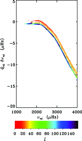
(a)   (b)

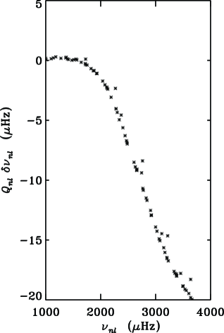
Figure 2: (a) Scaled differences between observed GONG frequencies and adiabatically computed frequencies of the ‘standard’ solar Model S. The degree $l$ of the oscillation modes is indicated by the colour bar. Image reproduced with permission from Christensen-Dalsgaard et al. (1996), copyright by AAAS. (b) Scaled adiabatic frequency differences between a model for which the near-surface layers were represented by a hydrodynamical simulation, and the ‘standard’ solar Model S, which does not include the turbulent pressure. Image adapted from Rosenthal et al. (1995).

Convection modifies pulsation properties of stars principally through two effects: (i) dynamical effects through the additional turbulent pressure term $p_{\mathrm{t}}$ (12) in the mean momentum equation (22), and its perturbation $\delta p_{\mathrm{t}}$ (73), (92), where $\delta$ denotes here a linear perturbation in a Lagrangian-mean frame of reference, in the pulsationally perturbed mean momentum equation; (ii) nonadiabatic effects, additional to the perturbed radiative heat flux $\delta\bm{F}_{\mathrm{r}}$, through the perturbed convective heat (enthalpy) flux $\delta\bm{F}_{\mathrm{c}}$ (72), (92) in the pulsationally perturbed mean thermal heat (energy) equation.

5.1 The effect of the Reynolds stress in the equilibrium stellar model

From the discussion before we conclude that the details of modelling the hydrostatic equilibrium structure in the near-surface layers play an important role in describing the residuals between observed and modelled oscillation frequencies, particularly for modes with $\nu$ close to $\nu_{\mathrm{ac}}$. Almost all stellar model calculations consider only the gradient of the gas pressure $p$ in the equation of hydrostatic support. In the convectively unstable surface layers, however, the additional contribution from the turbulent pressure $p_{\mathrm{t}}$ (12) to the hydrostatic support can be significant [see, e.g., Eq. (22)]. Hydrodynamical simulations of stellar convection have enabled us to estimate this contribution from the turbulent pressure $p_{\mathrm{t}}$. Figure 3 shows $p_{\mathrm{t}}$ for three different simulations and models of the Sun. It indicates that $p_{\mathrm{t}}$ can be as large as 15% of the total pressure $\hat{p}=p+p_{\mathrm{t}}$.

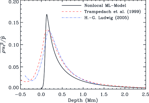
Figure 3: Turbulent pressure $p_{\mathrm{t}}:=\overline{\rho u^{2}_{r}}$ over total pressure $\hat{p}=p+p_{\mathrm{t}}$ as a function of the depth variable $R_{\odot}-r$ for various solar simulations and models ($R_{\odot}$ is the photospheric solar radius). Results are shown for the nonlocal mixing-length model of Section 3.3.1 by Gough (1977a, b, solid curve) and from hydrodynamical simulations by Regner Trampedach (1999, personal communication, dashed curve) and H.-G. Ludwig (2005, personal communication, dot-dashed curve).

Rosenthal et al. (1995), for example, investigated the effect of the contribution that $p_{\mathrm{t}}$ makes to the mean hydrostatic stratification on the adiabatic solar eigenfrequencies. They examined a hydrodynamical simulation by Stein and Nordlund (1991) of the outer 2% by radius of the Sun, matched continuously in sound speed to a model envelope calculated, as in a ‘standard’ solar model, with a local mixing-length formulation without $p_{\mathrm{t}}$. The resulting frequency shifts of adiabatic oscillations between the simulations and the ‘standard’ solar reference model, Model S, are illustrated in Figure 2b. The frequency residuals behave similarly to the solar data depicted in the left panel of that figure, though with larger frequency shifts at higher oscillation frequencies.

If turbulent pressure is considered in the mean structure, however, additional assumptions have to be made about the turbulent pressure perturbation in the adiabatic pulsation equations. The first adiabatic exponent $\gamma_{1}=(\partial\ln p/\partial\ln\rho)_{s}$ ($s$ being the specific entropy), is a purely thermodynamic quantity and is expressed by means of the gas pressure $p$. Consequently, in the presence of turbulent pressure $p_{\mathrm{t}}$, such that the total pressure $\hat{p}=p+p_{\mathrm{t}}$ satisfies the equation of hydrostatic equilibrium, $\gamma_{1}$ experiences a modification of the form

$$\gamma_{1}=\left(\frac{\partial\ln\hat{p}}{\partial\ln\rho}\right)_{\!\!s}=\frac{1}{\hat{p}}\left[\left(\frac{\partial p}{\partial\ln\rho}\right)_{\!\!s}+\left(\frac{\partial p_{\mathrm{t}}}{\partial\ln\rho}\right)_{\!\!s}\right]$$ (126)

and the relative Lagrangian perturbation in the total pressure is

$$\frac{\delta\hat{p}}{\hat{p}}=\frac{\delta p}{\hat{p}}+\frac{\delta p_{\mathrm{t}}}{\hat{p}}=\gamma_{1}\,\frac{\delta\rho}{\rho}\,.$$ (127)

Nonadiabatic pulsation calculations with the inclusion of the turbulent pressure perturbation $\delta p_{\mathrm{t}}$ (Houdek, 1996), and hydrodynamical simulation results (Rosenthal et al., 1995, 1999) indicate that $\delta p_{\mathrm{t}}$ varies approximately in quadrature with the other terms in the linearized momentum equation, and hence contributes predominantly to the imaginary part of the frequency shift, i.e., to the linear damping rate. The Lagrangian gas-pressure perturbation $\delta p$, however, responds adiabatically. Therefore, $\delta p_{\mathrm{t}}$ can be neglected in Eq. (127), i.e., in the calculation of the (real) adiabatic eigenfrequencies it is assumed that $\delta\hat{p}/\hat{p}\simeq\delta p/\hat{p}\simeq\tilde{\gamma}_{1}\delta\rho/\rho$. With this assumption $\tilde{\gamma}_{1}\simeq(p/\hat{p})\gamma_{1}$, and the only modification to the adiabatic oscillation equations is the replacement of $\gamma_{1}$ by $\tilde{\gamma}_{1}$ (Rosenthal et al., 1995).

5.2 The effects of nonadiabaticity and momentum flux perturbation

The effects of nonadiabaticity and convection dynamics on the pulsation frequencies were, for example, studied by Balmforth (1992b); Rosenthal et al. (1995) and Houdek (1996). In these studies, the nonlocal, time-dependent generalization of the mixing-length formulation by Gough (1977a, b) was adopted to model the heat and momentum flux consistently in both the equilibrium envelope model and in the nonadiabatic stability analysis. Houdek (1996) considered the following models:

• A local mixing-length formulation without turbulent pressure $p_{\mathrm{t}}$ was used to construct the mean envelope model. Frequencies were computed in the adiabatic approximation assuming $\delta p_{\mathrm{t}}=0$.

• Gough77a,Gough77b nonlocal, mixing-length model, including turbulent pressure, was used to construct the mean envelope model. Frequencies were computed in the adiabatic approximation assuming $\delta p_{\mathrm{t}}=0$.

• The mean envelope model was constructed as in NL.a. Nonadiabatic frequencies were computed including consistently the Lagrangian perturbations of the convective heat flux $\delta\bm{F}_{\mathrm{c}}$, additionally to $\delta\bm{F}_{\mathrm{r}}$, and turbulent momentum flux $\delta p_{\mathrm{t}}$.

  Additional care was necessary when frequencies between models with different convection treatments were compared, such as in the models L.A and NL.a. In order to isolate the effect of the near-surface structures on the oscillation frequencies the models had to posses the same stratification in their deep interiors. This was obtained by requiring the models to lie on the same adiabat near the base of the (surface) convection zone and to have the same convection-zone depth. Varying the mixing-length parameter $\alpha=\ell/H_{\mathrm{p}}$ and hydrogen abundance by iteration in model L.a, the same values for temperature and pressure were found at the base of the convection zone as those in models NL.a and NL.na. The radiative interior of the nonlocal models NL.a and NL.na were then replaced by the solution of the local model L.a, and the convection-zone depth was calibrated to $0.287\,R_{\odot}$ (Christensen-Dalsgaard et al., 1991). Further details of the adopted physics in the model calculations can be found in Houdek et al. (1999a).

  The outcome of these calculations is shown in Figure 4a. As for the hydrodynamical simulations (Figure 2b) the effect of the Reynolds stresses in the mean structure decreases the adiabatic frequencies (NL.a-L.a, solid curve) for frequencies larger than about 2 mHz, though the maximum deficit of about $12~{}\mu\mathrm{Hz}$ is smaller than in the hydrodynamical simulations. The effects of nonadiabaticity ($\delta\bm{F}_{\mathrm{r}}+\delta\bm{F}_{\mathrm{c}})$ and $\delta p_{\mathrm{t}}$ (NL.na-NL.a, dashed curve), however, lead to an increase of the mode frequencies by as much as $\sim 9~{}\mu\mathrm{Hz}$, nearly cancelling the downshifts from the effect of $p_{\mathrm{t}}$ in the mean structure, as illustrated by the dot-dashed curve (NL.na-L.a).

  (a)   (b)

  
  

  Figure 4: Frequency residuals between stellar models calculated with Gough’s nonlocal time-dependent mixing-length formulation (Section 3.3). (a) Results are shown for solar models: the solid curve (NL.a-L.a) shows the adiabatic radial oscillation frequency shifts, under the assumption $\delta p_{\mathrm{t}}=0$, caused by the turbulent pressure $p_{\mathrm{t}}$ in the mean envelope. The dashed curve (NL.na-NL.a) is the frequency shift caused by nonadiabaticity and effects of including consistently $\delta p_{\mathrm{t}}$. The overall frequency shift (NL.na-L.a) is plotted by the dot-dashed curve. (b) Results are shown for models for the solar-like star $\eta$ Boo. The model calculations and line styles are as in panel (a). Images reproduced from Houdek (1996).

  If, however, the positive frequency shifts between models NL.na and NL.a (dashed curve) are interpreted as the nonadiabatic and momentum flux corrections to the oscillation frequencies then their effects are to bring the frequency residuals of the hydrodynamical simulations (Figure 2b) in better agreement with the data plotted in Figure 2a.

  The effects of the near-surface regions in the Sun were also considered by Rosenthal et al. (1999) and Li et al. (2002) based on hydrodynamical simulations.

  A similar conclusion as in the solar case was found for the solar-like star $\eta\,$Boo by Christensen-Dalsgaard et al. (1995) and Houdek (1996), demonstrated in Figure 4b, and more recently by Straka et al. (2006). Grigahcène et al. (2012) studied the surface effects in the Sun and in three solar-type stars with the conclusion that the use of the local time-dependent convection treatment of Section (3.4) reduces the frequency residuals between observations and stellar models. In these calculations, however, the hydrostatic equilibrium model was corrected a posteriori by the effect of the mean turbulent pressure with some consequent inconsistencies in the thermal equilibrium structure.

  The near-surface frequency corrections also affect the determination of the modelled mean large frequency separation $\Delta\nu:=\langle\nu_{n+1l}-\nu_{nl}\rangle$ (angular brackets indicate an average over $n$ and $l$). In both models for the Sun (Christensen-Dalsgaard and Gough, 1980) and for $\eta\,$Boo the resulting corrections to $\Delta\nu$ are about $-1~{}\mu\mathrm{Hz}$. Although this correction is less than 1% it does affect the determination of the stellar radii and ages from the observed values of $\Delta\nu$ and small frequency separation $\delta\nu_{02}$ in distant stars.

  A simple procedure for estimating the near-surface frequency corrections was suggested by Kjeldsen et al. (2008). It is based on the ansatz that the frequency shifts can be scaled as $a(\nu/\nu_{0})^{b}$ (Christensen-Dalsgaard and Gough, 1980), where $\nu_{0}$ is a suitable reference frequency, $b$ is obtained from solar data, and the surface-correction amplitude $a$ is determined from fitting this expression to the observed frequencies.

  Kjeldsen et al.’s empirical power-law has been applied to the modelling of a large number of solar-type Kepler stars (e.g., Metcalfe et al., 2012; Mathur et al., 2012; Gruberbauer et al., 2013; Metcalfe et al., 2014). Mathur et al., for example, determined statistical properties of the surface-correction amplitude $a$ from 22 Kepler stars. The model frequencies were, however, obtained in the adiabatic approximation neglecting, as did Metcalfe et al. (2012) and Metcalfe et al. (2014), any convection dynamics in both the equilibrium and pulsation calculations. Mathur et al. (2012) concluded that the surface-correction amplitude $a$ is nearly a constant fraction of the mean large-frequency separation $\Delta\nu$. Information like this could provide additional insight into the physical processes responsible for the high radial-order frequency shifts between observations and stellar models. Gruberbauer et al. (2013, see also , ) analysed the surface effects in 23 Kepler stars with a Bayesian approach neglecting, however, convection dynamics in both the equilibrium and in the nonadiabatic eigenfrequency calculations.

  Christensen-Dalsgaard (2012) suggested an improved functional form for the high-order frequency shifts between observations and stellar models. This improved functional form can be determined for the Sun from the surface term in Duvall’s differential form for the asymptotic expression for frequencies using a large range of mode degrees $l$. This leads to a better representation of the solar frequency residuals brought about by the very surface layers. By adopting the acoustic cutoff frequency as the relevant frequency scale the scaled solar-surface functional form can also be applied to other stars that are not too dissimilar to the Sun. Christensen-Dalsgaard (2012) applied it to Kepler data for the solar-type star 16 Cyg A and reported a better representation of the frequency surface correction compared to the empirical power law by Kjeldsen et al. (2008). Another empirical approach was recently reported by Ball and Gizon (2014), which is based on the scaling relation for mode inertia by Gough (1990).

  Although these empirical approaches offer some description of the surface effects, they do not provide the much needed insight for describing the relevant physical processes. The most promising approach today for a better understanding of these surface effects is the use of the latest implementations of three-dimensional (3D) hydrodynamical simulations, and their results, for developing improved one-dimensional (1D) convection models. Several international groups are now pursuing this approach.

  6 Driving and Damping Mechanisms

  The question of whether the amplitude (or energy) of a particular oscillation mode in a star is growing or declining with time is related to the problem of vibrational stability. Because vibrational stability (or instability) is characterized by the existence of a periodicity in the temporal behaviour of the perturbations, a reasonable useful criteria is the sign of the total energy change (thermal and mechanical) over one pulsation period assuming that the system returns precisely to its original state at the end of the period. This is the definition of the work integral $W$.

  6.1 The work integral

  6.1.1 Expressions for radial pulsations

  It was Eddington (1926), who recognized first that a non-vanishing expression for the work integral $W$, which is of second order in the pulsation quantities, can be obtained from the vanishing expression of the integrated (specific) entropy, $s$, over one pulsation period, i.e., from $\oint\,\mathrm{d}s=0$, because $s$ is a state variable. For the nonadiabatic contributions $W$ is obtained from the (linearly) perturbed thermal energy equation (3). Recognizing that $\rho\,\mathrm{d}e/\,\mathrm{d}t+p\nabla\cdot\bm{v}=\rho T\,\mathrm{d}s/\,\mathrm{d}t$, where $\,\mathrm{d}/\,\mathrm{d}t$ is the substantial (or material) derivative in a frame with (total) velocity $\bm{v}$, we obtain

  $$W=\int_{0}^{M}\,\mathrm{d}m\oint\delta T\frac{\partial\delta s}{\partial t}\,\mathrm{d}t\,,$$ (128)

  for a star with zero gas pressure $p$ at the stellar surface $r=R$ and mass $M$. The boundary condition, $p=0$ at the surface $R$, expresses that no work ($\int_{A}p\,\bm{U}\cdot\,\mathrm{d}\bm{A}=0$, $\bm{A}$ is the star’s surface area, and $\bm{U}$ is the pulsation velocity) is exerted from outside, i.e., from layers with radius $r>R$. If $W>0$ the energy (pulsation amplitude) increases with time and consequently the pulsation mode is unstable or overstable. For $W<0$ the mode is said to be (intrinsically) stable or damped.

  Alternatively, one can also interpret the work integral $W$ as the amount of energy that is required to be added to (damped, stable mode) or subtracted from (unstable mode) the pulsating system to maintain exact periodicity. This concept was adopted by Baker and Kippenhahn (1962, 1965), who started from the expression for the work done on the (stellar) sphere with volume $V$ during one pulsation period, i.e.,

  $$W=-\oint p\,\frac{{\partial}V}{{\partial}t}\,\mathrm{d}t=-\oint p\,\bm{U}\cdot\,\mathrm{d}\bm{A}\,\mathrm{d}t\,.$$ (129)

  From this expression they derived the work integral

  $$W_{\mathrm{g}}=\pi\int_{0}^{M}\frac{1}{\rho^{2}}\Im\left({\delta p^{\ast}\delta\rho}\right)\,\mathrm{d}m\,,$$ (130)

  associated with the gas pressure $p$, for radial pulsations without convection dynamics and under the assumption that the imaginary part, $\omega_{\mathrm{i}}=\Im\left({\omega}\right)$, of the complex pulsation eigenfrequency, $\omega$, vanishes; the asterisk denotes complex conjugate.

  Baker and Gough (1979) considered the fully nonadiabatic linearized stability problem for radial modes with the inclusion of convection dynamics by adopting the local time-dependent convection model of Section (3.2.3). Their derivation of the work integrals starts from the pulsationally linearized form of the mean momentum equation (9) which, after multiplication by the complex conjugate of the radial component $\xi_{\mathrm{r}}=:\delta r$ of the displacement vector $\bm{\xi}$, leads to the work-integral contribution from the turbulent pressure $p_{\mathrm{t}}$

  $$W_{\mathrm{t}}(m) = \pi\int_{m_{\mathrm{b}}}^{M_{\star}}\Im(\delta p_{\mathrm{t}}\,^{\ast}\,\delta\rho)\frac{\,\mathrm{d}m}{\rho^{2}}$$ (131)

  $$+ \pi\int_{m_{\mathrm{b}}}^{M_{\star}}\Biggl{\{}(3-\Phi)\left[\Im(\delta r\,^{\ast}\,\delta p_{\mathrm{t}})-\frac{p_{\mathrm{t}}}{\rho}\Im(\delta r\,^{\ast}\,\delta\rho)\right]-p_{\mathrm{t}}\Im(\delta r\,^{\ast}\,\delta\Phi)\Biggr{\}}\frac{\,\mathrm{d}m}{\rho r}\,,$$ (132)

  additionally to expression (130) for the gas-pressure contribution $W_{\mathrm{g}}$, but with the lower integration boundary replaced by the mass $m_{\mathrm{b}}$ at the bottom boundary of the stellar envelope model. The complex pulsation frequency $\omega=\omega_{\mathrm{r}}+\mathrm{i}\,\omega_{\mathrm{i}}$ is then related to the work integrals by

  $$\frac{\omega_{\mathrm{i}}}{\omega_{\mathrm{r}}}=\frac{W_{\mathrm{g}}+W_{\mathrm{t}}+F}{2\pi\omega^{2}_{\mathrm{r}}\int_{m_{\mathrm{b}}}^{M}|\delta r|^{2}\,\mathrm{d}m}:=\frac{-\eta_{\mathrm{g}}-\eta_{\mathrm{t}}+\tilde{F}}{\omega_{\mathrm{r}}}:=\hat{\eta}_{\mathrm{g}}+\hat{\eta}_{\mathrm{t}}+\hat{F}\,,$$ (133)

  where $\eta_{\mathrm{g}}$ and $\eta_{\mathrm{t}}$ are respectively the linear damping rates of the gas and turbulent pressure contributions, $\hat{\eta}_{\mathrm{g}}$ and $\hat{\eta}_{\mathrm{t}}$ are the associated stability coefficients, and $F:=\left[4\pi^{2}r^{2}\Im({\delta p^{\ast}\delta r})\right]^{M}_{m_{\mathrm{b}}}$ is typically negligible.

  6.1.2 Expressions for nonradial pulsations

  Expressions of work integrals for nonradial pulsations were reported by, e.g., Grigahcène et al. (2005) in the framework of applying the time-dependent convection model of Section 3.4 to several classes of pulsating stars. As before, the work integrals can be obtained by taking the scalar product of the linearly perturbed average momentum equation with the displacement vector $\bm{\xi}^{\ast}$, followed by integration by part over the total stellar mass and considering only the imaginary part of the final result, which is:

  $$\omega_{\mathrm{i}} = \frac{\displaystyle{\int_{0}^{M}\Im\left\{\frac{{\delta\rho}}{\rho}\frac{\delta\hat{p}^{*}}{\rho}+\,\mathrm{d}W_{\mathrm{Rey}}\right\}\,\mathrm{d}m}}{2\,\omega_{\mathrm{r}}\int_{0}^{M}{\left|\bm{\xi}\right|}^{2}\,\mathrm{d}m}\,,$$ (134)

  where $\Im\{{\delta\rho}\delta\hat{p}^{*}/\rho^{2}\}$ and $\,\mathrm{d}W_{\mathrm{Rey}}\simeq\left(\xi_{\mathrm{r}}^{*}\Xi_{\mathrm{r}}+l(l+1)\xi_{\mathrm{h}}^{*}\Xi_{\mathrm{h}}\right)/\rho$ are the work contributions per unit mass produced during one pulsation cycle by the total (gas + radiation + turbulence) pressure $\hat{p}$ and by the non-diagonal components of the Reynolds stress tensor, respectively, and $\Xi_{\mathrm{r}}$ and $\Xi_{\mathrm{h}}$ are defined in Eq. (191). As for the radial case the work produced by the total pressure can be separated into contributions from the gas and radiation pressure ($p$) and from the turbulent pressure ($p_{\mathrm{t}}$), i.e.,

  $$\Im\left\{\frac{{\delta\rho}}{\rho}\frac{\delta\hat{p}^{*}}{\rho}\right\} = \Im\left\{\frac{{\delta\rho}}{\rho}\frac{\delta p^{*}}{\rho}\right\}+\,\mathrm{d}W_{\mathrm{t}}\,,$$ (135)

  where $\,\mathrm{d}W_{\mathrm{t}}=\Im\{{\delta\rho}\delta p_{\mathrm{t}}^{*}/\rho^{2}\}$ is the work by the turbulent pressure. From the equations of state and energy conservation we obtain for the contribution of the gas (and radiation) pressure

  $$\Im\left\{\frac{{\delta\rho}}{\rho}\frac{\delta p^{*}}{\rho}\right\} = \,\mathrm{d}W_{\mathrm{FR}}+\,\mathrm{d}W_{\mathrm{FC}}+\,\mathrm{d}W_{\epsilon_{\mathrm{t}}}\,,$$ (136)

  where $W_{\mathrm{FR}}$, $W_{\mathrm{FC}}$ and $W_{\epsilon_{\mathrm{t}}}$ are the contributions from the radiative and convective heat flux, and from the dissipation of turbulent kinetic energy, respectively. For simplicity we neglect in the next equations the terms corresponding to the horizontal component of the flux divergence. These terms are very small because the pressure and temperature scale heights are much smaller compared to the term, $r/l$, for modes with low spherical degree $l$, and we also neglect the nuclear reactions. We then obtain

  $$\,\mathrm{d}W_{\mathrm{FR}}+\,\mathrm{d}W_{\mathrm{FC}}=-\Re\left\{\frac{{\delta T}^{*}}{T\omega}\frac{\,\mathrm{d}\,\delta\left(L_{\mathrm{R}}+L_{\mathrm{c}}\right)}{\,\mathrm{d}m}\right\}\,,$$ (137)

  and for the last term in Eq. (136), which is the contribution from the viscous dissipation of turbulent kinetic energy into heat, we obtain, after neglecting the contributions of the last geometrical term in Eq. (120), the work contribution

  $$\,\mathrm{d}W_{\epsilon_{\mathrm{t}}}\;\simeq\;-({\gamma_{3}}-1)\frac{{\Phi}}{2}\Im\left\{\frac{{\delta\rho}}{\rho}\frac{\delta p_{\mathrm{t}}^{*}}{\rho}\right\}\,,$$ (138)

  where $\gamma_{3}$ is the third adiabatic exponent defined as $\gamma_{3}-1:=(\partial\ln T/\partial\ln\rho)_{s}$, and $s$ is the specific entropy. As noted by Ledoux and Walraven (1958) and Grigahcène et al. (2005), the terms $\,\mathrm{d}W_{\mathrm{t}}$ and $\,\mathrm{d}W_{\epsilon_{\mathrm{t}}}$ cancel exactly for a completely ionized gas without radiation (${\gamma_{3}}-1=2/3$) and for isotropic turbulence (${\Phi}=3$).

  It should be noted that in Gough77a, Gough77b convection model the viscous dissipation by turbulent kinetic energy into heat is neglected in the thermal energy equation, as suggested by Spiegel and Veronis (1960) for a (static, i.e., $\bm{U}=\bm{0}$) Boussinesq fluid.

  In the following sections, we shall review and compare results of stability calculations between the two time-dependent convection formulations by Gough (1977a, b) and Grigahcène et al. (2005) for various classical pulsators and for stars with stochastically excited oscillations.

  6.2 Intrinsically unstable pulsators

  One of the most prominent stability computations in stars has been the modelling of the location of the classical instability strip in the Hertzsprung–Russell diagram. Since the seminal work by Baker and Kippenhahn (1962, 1965) for modelling linear stability coefficients in Cepheids, various attempts have been made to reproduce theoretically the observed location of the instability strip. The properties of the hotter, blue edge of the instability strip could be explained first (e.g., Castor, 1970; Petersen and Jørgensen, 1972; Dziembowski and Kozlowski, 1974; Stellingwerf, 1979, and references therein), mainly because for these hotter stars the rather thin surface convection zone does not affect pulsation dynamics too severely. The modelling of the return to pulsational stability at the cooler, red edge, however, has been less successful, despite the first promising attempts by, e.g., Deupree (1977a), who solved the nonlinear hydrodynamic equations, using a time-varying eddy viscosity, for studying the stability properties of RR Lyrae stars. The need for a time-dependent convection treatment for modelling the low-temperature, red edge of the instability strip was recognized by Baker and Kippenhahn (1965, see also , ).

  6.2.1 Cepheids and RR Lyrae stars

  The first theoretical studies describing successfully the location of the cool edge of the classical Cepheid instability strip were reported by Baker and Gough (1979) for RR Lyrae stars, using linear stability analyses of radial modes and the local time-dependent convection formulation of Section 3.2.3. Shortly thereafter, Xiong (1980) was successful with Cepheid models, using his own local time-dependent convection model (Xiong, 1977, see Section 4). In the same year Gonczi and Osaki (1980) used Unno’s (1967, see Section 3.2.3) time-dependent convection model for analysing stability properties of Cepheid models, but only with the inclusion of an additional scalar turbulent viscosity, brought about by the small-scale turbulence [see Eq. (139)], could Gonczi (1981) successfully model the return to stability near the cool edge of the instability strip.

  Later, Stellingwerf (1986), using Stellingwerf82 turbulence formulation with a simplified extension for one-zone pulsation models (Baker, 1966; Baker et al., 1966), conducted linear and nonlinear Cepheid stability analyses. He reported that the coupling between pulsation and convection can describe a return to stability for cooler Cepheid models. In this study, however, the effect of turbulent pressure was omitted in the calculations, but later included by Munteanu et al. (2005), who concluded that the turbulent pressure appears to be a driving mechanism. Nonlinear pulsation modelling of Cepheids, using the nonlocal, time-dependent, one-equation, convection formulation by Kuhfuß (1986), were reported by Smolec and Moskalik (2008); Buchler (2009), and Smolec and Moskalik (2010).

  Linear stability analyses of radial Cepheid pulsations were also conducted by Balmforth and Gough (1988), using Gough77a local convection model of Section 3.2.3. Houdek et al. (1999b) discussed linear stability analyses and nonadiabatic pulsation-period ratios in double-mode Cepheids, using Gough77b nonlocal convection formulation of Section 3.3.2. Both studies reproduced the cool edge of the classical instability strip, with the pulsationally perturbed turbulent pressure being the main contributor for stabilizing the pulsation modes. Yecko et al. (1998), on the other hand, found the damping effect of the small-scale turbulent eddy viscosity (see Eq. 139) to be the main agent for making the pulsation modes stable at the cool side of the instability strip. The authors adopted the convection model by Gehmeyr (1992), which is based on Stellingwerf82 turbulence model, for their linear stability computations.

  6.2.2 Mira variables

  Mira variables are long-period variables (LPV) with radial pulsation periods $P\gtrsim 80\mathrm{\ days}$ located to the red of the classical instability strip with typical surface temperatures between 2500 and 3500 K and luminosities between $\sim 10^{3}$ and $\sim 7\times 10^{3}\,\mathrm{L}_{\odot}$. The detailed driving mechanism of these low-order radial oscillations depends crucially on the treatment of the coupling of the pulsations to the convection. Several attempts have been made in the past to model this coupling in both linear and nonlinear calculations with rather oversimplified descriptions (e.g., Kamijo, 1962; Keeley, 1970; Langer, 1971; Cox and Ostlie, 1993). The first attempt to describe the coupling in a more realistic way was conducted by Gough (1966, 1967), who included the pulsational perturbations of both the convective heat (enthalpy) flux $\delta F_{\mathrm{c}}$ and momentum flux $\delta p_{\mathrm{t}}$ in the linear stability analyses. Gough concluded that in particular the momentum flux perturbation $\delta p_{\mathrm{t}}$ has a stabilizing effect on the pulsations if the pulsation period is much shorter than the characteristic time scale of the convection, whereas for long-period pulsations, such as in Mira variables or supergiants, the turbulent pressure fluctuations $\delta p_{\mathrm{t}}$ destabilizes (drives) the stellar pulsations. It is perhaps interesting to note that a similar effect was noticed in linear Delta Scuti stability computations by Houdek (1996) and more recently by Antoci et al. (2014) (see Section 6.2.3), in which $\delta p_{\mathrm{t}}$ was found to drive high-order radial pulsations, in agreement with observations. Using the local time-dependent formulation by Gough (1977a), Balmforth et al. (1990) concluded that including the turbulent pressure in the mean model of Mira variables modifies the equilibrium structure such as to make the observed radial pulsations overstable in the pulsation computations which is, however, partially offset by the stabilizing influence of $\delta p_{\mathrm{t}}$. Xiong et al. (1998), on the other hand, found $\delta p_{\mathrm{t}}$, together with the turbulent eddy viscosity [see Eq. (139)], to be the main stabilizing contribution to linear Mira pulsations. Munteanu et al. (2005) and Olivier and Wood (2005) conducted nonlinear pulsation models using the one-equation turbulence models by Stellingwerf (1986) and Kuhfuß (1986) respectively, and reported about the destabilizing effect of $\delta p_{\mathrm{t}}$, i.e., in accordance with the earlier findings by Gough (1966, 1967). It appears that further progress on modelling the interaction between convection and pulsations in Mira variables is required.

  

  Figure 5: Mode stability of an $1.7\,M_{\odot}$ Delta Scuti star computed with Gough77a, Gough77b convection model. Left: Stability coefficient $\hat{\eta}=\omega_{\mathrm{i}}/\omega_{\mathrm{r}}$ as a function of surface temperature $T_{\mathrm{eff}}$ across the instability strip. Results are shown for the fundamental radial mode ($n=1$). Positive $\hat{\eta}$ values indicate mode instability. The separate contributions to $\hat{\eta}$ arising from the gas pressure perturbations, $\eta_{\mathrm{g}}$, and from the perturbation of the momentum flux, $\eta_{\mathrm{t}}$, with $\eta=\eta_{\mathrm{g}}$+ $\eta_{\mathrm{t}}$, are obtained from the evaluation of the work integral (133). Right: Integrated work integral $W$ as a function of the depth co-ordinate $\log(T)$ for a model lying just outside the cool edge of the instability strip (surface temperature $T_{\mathrm{eff}}=6813\mathrm{\ K}$). Results are plotted in units of $\hat{\eta}$. Contributions to $W$ (solid curve) arising from the gas pressure perturbation, $W_{\mathrm{g}}$ (dashed curve), and the turbulent pressure perturbations, $W_{\mathrm{t}}$ (dot-dashed curve), are illustrated ($W=W_{\mathrm{g}}+W_{\mathrm{t}}$). The dotted curve is the ratio of the convective to the total heat flux ${F_{\mathrm{c}}/F}$. Ionization zones of H and He (5% to 95% ionization) are indicated (from Houdek, 2000).

  6.2.3 Delta Scuti stars

  Already before the successful space missions CoRoT (Baglin et al., 2009) and Kepler (Christensen-Dalsgaard et al., 2009a) several observing campaigns, e.g., the Delta Scuti Network (DNS) or the Whole Earth Telescope (WET), have been providing excellent oscillation data of Delta Scuti stars. For example, Breger et al. (1999) identified 24 pulsation frequencies in the Delta Scuti star FG Vir. Such high-quality seismic data also provided well-defined observed locations of the lower part of the classical instability strip (e.g., Rodríguez et al., 2000), which modellers could use to test their time-dependent convection models.

  For example, Houdek et al. (1999a) reported linear stability results about the locations of the lower instability strip for the fundamental and first overtone radial modes. For one of these models, detailed stability computations were reported by Houdek (2000). These computations included consistently the Reynolds stresses in both the equilibrium envelope models [$p_{\mathrm{t}}$ in Eq. (22)] and in the linear pulsation calculations ($\delta p_{\mathrm{t}}$, Eqs. 73, 92). The left panel of Figure (6.2.2) displays the stability coefficient $\hat{\eta}:=\omega_{\mathrm{i}}/\omega_{\mathrm{r}}$ ($\omega=\omega_{\mathrm{r}}+\mathrm{i}\omega_{\mathrm{i}}$) of the fundamental mode (solid curve) for an evolving $1.7\,M_{\odot}$ Delta Scuti star crossing the lower instability strip. The individual contributions from the gas (and radiation) pressure, $\eta_{\mathrm{g}}$ (dashed curve), and (perturbed) turbulent pressure, $\eta_{\mathrm{t}}$ (dot-dashed curve), are indicated. The return to stability ($\hat{\eta}<0$) near the red edge, at about 6895 K, is entirely determined by the turbulent pressure contribution $\eta_{\mathrm{t}}$ to the work integral. Another way to demonstrate this result is to analyse the work integral $W$. The right panel of Figure 6.2.2 shows $W$ and its individual contributions $W_{\mathrm{g}}$ [dashed curve; see Eq. (130)] and $W_{\mathrm{t}}$ [dot-dashed curve; see Eq. (132)] for a stellar model (with a surface temperature $T_{\mathrm{eff}}=6799\mathrm{K}$) located just outside the red edge of the instability strip. From this it is obvious that the dominating damping term to the work integral $W$ is the contribution from the turbulent pressure perturbations $W_{\mathrm{t}}$ (dot-dashed curve with negative value at the stellar surface), whereas the gas (and radiation) pressure contribution $W_{\mathrm{g}}$ (dashed curve) contribute to the driving (positive value at the stellar surface).

  

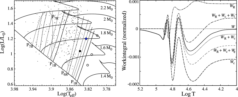
  Figure 6: Stability computations of Delta Scuti stars, which include the viscous dissipation rate $\epsilon_{\mathrm{t}}$ of turbulent kinetic energy according to Grigahcène et al. (2005). Left: Blue and red edges of the instability strip superposed on evolutionary tracks on the theorists Hertzsprung–Russel diagram. The locations of the edges, labelled $\mathrm{p}_{n\mathrm{B}}$ and $\mathrm{p}_{n\mathrm{R}}$, are indicated for radial modes with orders $1\leq n\leq 7$. Results by Houdek (2000, $\alpha=2.0$, see Figure 6.2.2) and Xiong and Deng (2001) for the gravest p modes are plotted as filled and open circles respectively. The small dots are observed Delta Scuti Stars (Rodríguez et al., 2000). Right: Integrated work integral $W$ as a function of the depth co-ordinate $\log(T)$ for a stable $n=3$ radial mode of a $1.8\,M_{\odot}$ star (see ‘star’ symbol in the left panel). Contributions to $W$ arising from the radiative flux, $W_{\mathrm{R}}$, the convective flux, $W_{\mathrm{c}}$, the turbulent pressure perturbations, $W_{\mathrm{t}}$ ($W_{\mathrm{R}}+W_{\mathrm{c}}+W_{\mathrm{t}}$), and from the perturbation of the turbulent kinetic energy dissipation, $W_{\epsilon_{\mathrm{t}}}$ ($W_{\mathrm{R}}+W_{\mathrm{c}}+W_{\epsilon_{\mathrm{t}}}$), are indicated. Images adapted from Dupret et al. (2005c).

  Dupret et al. (2005c) used the local time-dependent convection treatment of Grigahcène et al. (2005, see Section 3.4), to study the stability properties of radial and nonradial pulsations in $\delta$ Sct stars. In these calculations the perturbations of both the convective heat flux $\delta F_{\mathrm{c}}$ and turbulent pressure $\delta p_{\mathrm{t}}$ were included in the linear pulsation computations, but the (mean) turbulent pressure $p_{\mathrm{t}}$ was omitted in the construction of the equilibrium structure. Dupret et al. (2005c) found well defined red edges of the instability strip for both radial and nonradial modes using Grigahcéne et al.’s time-dependent convection model. The authors found that the $\delta$ Sct low-order p modes become stable again with decreasing $T_{\mathrm{eff}}$ when the two thin convective zones, associated with the partial ionization of hydrogen and helium, merge to form one large surface convection zone. For a solar-calibrated mixing-length parameter $\alpha=\ell/H$ ($\ell$ is the mixing length and $H$ is the pressure scale height) the return to stability occurs at the observed location in the Hertzsprung–Russell diagram. For smaller values of $\alpha$ the calculated cool edge of the instability strip is shifted towards cooler surface temperatures $T_{\mathrm{eff}}$ (Dupret et al., 2005c), in accordance with the findings by Houdek (2000), i.e., the observed location of the red edge could be used to calibrate the mixing-length parameter.

  The results of Dupret et al.’s stability analysis for Delta Scuti stars are depicted in Figure 6. The left panel compares the location of the red edge with results reported by Houdek (2000, see also Figure 6.2.2) and Xiong and Deng (2001). The right panel of Figure 6 displays the individual contributions to the accumulated work integral $W$ for a star located near the red edge of the $n=3$ mode (indicated by the ‘star’ symbol in the left panel). It demonstrates the near cancellation effect between the contributions of the turbulent kinetic energy dissipation, $W_{\epsilon_{\mathrm{t}}}$, and turbulent pressure, $W_{\mathrm{t}}$, making the contribution from the perturbations of the convective heat flux, $W_{\mathrm{c}}$, the dominating damping term. Moreover, even calculations without the inclusion of $\delta p_{\mathrm{t}}$ in the stability analysis led to a definition of the theoretical red edge of the instability strip. This is in contrast to the finding by Houdek et al. (1999a) and Houdek (2000), who reported the turbulent pressure perturbations, $\delta p_{\mathrm{t}}$, as the main mechanism for defining the red edge of the instability strip.

  

  Figure 7: Accumulated work integral $W$ as a function of the depth co-ordinate $\log(p)$. Results are shown for the $n=1$ radial mode of a Delta Scuti star located inside the instability strip (left panel) and outside the red edge of the instability strip (right panel). The stability calculations include viscous dissipation by the small-scale turbulence (Xiong, 1989, see Eq. (139)). Contributions to $W$ (solid curve) arising from the gas pressure perturbations, $W_{\mathrm{g}}$ (dashed curve), the turbulent pressure perturbations, $W_{\mathrm{t}}$ (long-dashed curve), and from the turbulent viscosity, $W_{\nu}$ (dotted curve), are illustrated ($W=W_{\mathrm{g}}+W_{\mathrm{t}}+W_{\nu}$). The ionization zones of H and He are indicated. Images adapted from Xiong and Deng (2007).

  The convection model by Xiong (1977, 1989) uses transport equations for the second-order moments of the convective fluctuations (see Section 4). Similar to Gough (1977a, b), Xiong does not include a work integral for the viscous dissipation of turbulent kinetic energy, $W_{\epsilon_{\mathrm{t}}}$ (neither does Unno et al. (1989, $\mathsection$26, $\mathsection$30), but includes the viscous damping effect of the small-scale turbulence in his model. All the convection models described in this review consider only the largest, most energy-containing, eddies and ignore the dynamics of the small-scale eddies lying further down the turbulent cascade. Small-scale turbulence does, however, contribute directly to the turbulent fluxes and, under the assumption that they evolve isotropically, they generate an effective viscosity $\nu_{\mathrm{t}}$, which is felt by a particular pulsation mode as an additional damping effect. The turbulent viscosity can be estimated as (e.g., Gough, 1977b; Unno et al., 1989, $\mathsection$20) $\nu_{\mathrm{t}}\simeq\lambda(\overline{ww})^{1/2}\ell$, where $\lambda$ is a parameter of order unity. The associated work integral $W_{\nu}$ can be written in cartesian coordinates as (Ledoux and Walraven, 1958, $\mathsection$63)

  $$W_{\nu}=-2\pi\;\omega_{\mathrm{r}}\int_{m_{\mathrm{b}}}^{M}\nu_{\mathrm{t}}\left[e_{ij}e_{ij}-\frac{1}{3}\left(\nabla\cdot\bm{\xi}\right)^{2}\right]\,\mathrm{d}m\,,$$ (139)

  where $e_{ij}=(\partial_{j}\xi_{i}+\partial_{i}\xi_{j})/2$ and $\bm{\xi}$ is the displacement eigenfunction. Xiong and Deng (2001, 2007) modelled successfully the instability strip of Delta Scuti and red giant stars and found the dominating damping effect to be the turbulent viscosity (139). This is illustrated in Figure 7 for models of two Delta Scuti stars: one model is located inside the instability strip (left panel), the other model is located outside the cool edge of the instability strip (right panel). The contribution from the small-scale turbulence was also the dominant damping effect in the stability calculations by Xiong et al. (2000) of radial p modes in the Sun, although the authors still found unstable modes with radial orders between $11\leq n\leq 23$. In contrast, Balmforth (1992a), who adopted the convection model of Gough (1977a, b), found all solar p modes to be stable due mainly to the damping of the turbulent pressure perturbations, $W_{\mathrm{t}}$, and reported that viscous damping, $W_{\nu}$, is about one order of magnitude smaller than the contribution of $W_{\mathrm{t}}$. Small-scale turbulent viscosity (139) leads always to mode damping, where as the perturbation of the turbulent kinetic energy dissipation, $\updelta\epsilon_{\mathrm{t}}$, can contribute to both damping and driving of the pulsations (Gabriel, 1996). The driving effect of $\updelta\epsilon_{\mathrm{t}}$ was shown by Dupret et al. (2005b) for $\gamma$ Doradus stars (see Section 6.2.4).

  It is clear from the discussion above that all three time-dependent convection models (Gough, 1977a; Xiong, 1989; Grigahcène et al., 2005) are able to reproduce theoretically the red edge of the instability strip, and about at the same location as observations suggest. The very detailed physical processes, however, that lead to the definition of the red edge are different in all three convection models: Gough’s model predicts that it is the perturbed Reynolds stress, Xiong (1989) the viscous dissipation by the small-scale turbulence, and the model by Grigahcène et al. (2005) predicts that it is the perturbed convective heat flux, which is responsible for the return to stability.

  Form these results it is obvious that further research is necessary to identify the correct processes that define the location of the cool edge of the classical instability strip.

  6.2.4 Gamma Doradus stars

  $\gamma$ Dor stars are F-type g-mode pulsators located near the red edge of the $\delta$ Scuti instability strip. A driving mechanism for these modes was proposed by Guzik et al. (2000), who used a standard time-independent, or frozen, convection model. The time scale associated to convective motions is, however, shorter than the pulsation periods in most of the convective envelope $\gamma$ Doradus stars, and the validity of frozen convection models for estimating stability properties of oscillations is therefore doubtful in these stars. This motivated Dupret et al. (2004b) and Dupret et al. (2005a, b) to use the time-dependent convection treatment of Grigahcène et al. (2005) for studying the driving mechanisms in $\gamma$ Dor stars. The important result was that unstable g modes are also obtained with this time-dependent convection treatment, with a range of frequencies (from $\sim$ 0.3 to 3 days) in agreement with typical observations. The theoretical instability strip could be computed and good agreement with observations was obtained for certain values of the mixing-length parameter $\alpha$.

  In the study of nonadiabatic processes we generally define the transition region in a star as the region where the thermal relaxation time is of the same order as the pulsation period. This region generally plays the major role in the driving or damping (see e.g., Cox, 1974). Efficient driving of $\gamma$ Dor g modes occurs when much of the region lies just above the base of the convective envelope, for there the mode of heat transport changes dramatically. Because convection typically carries most of the heat, yet the flux is presumed to be frozen, it dams up heat when the radiative flux from below is relatively high and transmits more when the incident flux is low. The radiative component of the flux in the convection zone is essentially unchanged, aside from that resulting directly from the modification by convection of the mean thermal stratification. The process can drive the pulsations, and is often called “convective blocking”, a terminology that could be misleading. A more accurate term would be “convective shunting”, because convection essentially redistributes the radiative flux, thereby reducing the relative modulation by radiation of the total flux.

  For the mixing-length parameter $\alpha=2$, and adopting Grigahcène et al.’s convection model, the transition region and bottom of the convective envelope coincide for stellar models that are located in the Hertzsprung–Russell diagram where $\gamma$ Dor stars are observed. For smaller values of $\alpha$, stellar models with lower effective temperatures are required to have a sufficiently deep convective envelopes, i.e., the location of the theoretically determined instability strip is shifted to lower temperatures in the Hertzsprung–Russell diagram. An important issue that has not yet been fully studied is the role of the non-diagonal components of the Reynolds stress in the driving. Preliminary studies using the formulation of Gabriel (1987) indicate that it is important, but numerical instabilities make this problem very delicate (see also Gough and Houdek, 2001).

  6.2.5 Rapidly oscillating Ap stars

  Rapidly oscillating Ap stars (hereafter roAp stars) are main-sequence stars with typical masses between 1.5 and $2.0\,M_{\odot}$ and with effective temperatures $T_{\mathrm{eff}}$ between 6800 and 8400 K. They are the coolest stars amongst the chemically peculiar A-type (Ap) stars with high overabundances of Sr, Cr and Eu. They show strong, predominantly dipolar, large-scale magnetic fields with magnitudes varying typically from 1 to about 25 kG, leading to antipodal spots. The roAp stars have in general rotation periods larger than about two days. The periods of the light variability range from roughly 5 to 21 minutes and are interpreted as high-order, low-degree acoustic modes. The first roAp star was discovered photometrically by Kurtz (1978) and their number has increased today to about 43 (Kurtz et al., 2011). Recent reviews on roAp stars were given by Gough (2005); Cunha (2007), Shibahashi (2008) and Kochukhov (2009).

  The observed pulsation properties in roAp stars suggest that the pulsation axis is not aligned with the rotation axis. This had led to the so-called oblique pulsator model (Kurtz, 1982), in which the observed cyclically varying oscillation amplitudes are explained by dipole oscillations being aligned with the magnetic axis, which itself is oblique to the rotation axis of the star. The pulsation eigenfunction differs, however, from a simple spherical harmonic (e.g., Takata and Shibahashi, 1994, 1995; Montgomery and Gough, 2003; Saio and Gautschy, 2004). By taking into account the effects of rotation and magnetic field, Bigot and Dziembowski (2002) generalized the oblique pulsator model, suggesting that the pulsation axis can be located anywhere between the magnetic and rotation axis.

  Several models were suggested for the mechanism that drives the low-degree high-order acoustic modes to the relatively low (up to 6 mmag) observed amplitudes (for a review see, e.g., Houdek, 2003). In the first theoretical paper on roAp stars by Dolez and Gough (1982), the authors assumed a strong dipolar magnetic field which inhibits convection totally in the polar spot-like regions, whereas in the equatorial region the convection is unaffected. The high-order acoustic oscillations are excited by the $\kappa$ mechanism in the hydrogen layers of the radiative polar spot-like regions. This model was adopted by Balmforth et al. (2001) using updated opacity tables and the nonlocal, time-dependent convection model by Gough (1977a, b). Depending on the assumed size of the polar spot-like regions Balmforth et al. (2001) did find overstable, high-order, axisymmetric dipole modes and other overstable modes with increasing spot size.

  This encouraging result has led Cunha (2002) to model the instability strip for roAp stars, but the author concluded that the models cannot explain the presence of observed oscillations in the coolest roAp stars. Even if the metallicity is varied (Théado et al., 2009) the agreement between theory and observation could not be improved.

  Dolez and Gough (1982) also addressed the question why the axisymmetric oscillations should always be nearly aligned with the spots, even if those spots are located near the (rotational) equator. They proposed that the (essentially standing) eigenmodes of oscillation suffer retrograde Coriolis precession in a frame of reference rotating with the star, and are therefore excited to observable amplitudes by the $\kappa$ mechanism only if they are nearly aligned with the spots. A more detailed discussion on this model was recently presented by Gough (2012b).

  The theory of roAp stars is further complicated by the still not fully understood mechanism that limits the pulsation amplitudes to the rather small values of $\lesssim$ 6 mmag, compared to the amplitudes of classical pulsators such as Cepheids or Delta Scuti stars. A possible explanation could be energy dissipation in the higher atmospheric layers brought about by shocking characteristics leading to steepening of the eigenfunctions which can then be thought of as a temporally harmonic series (Gough, 2013), with the high harmonics propagating farther out into the atmosphere where they dissipate the energy. Obviously, there is still much more to investigate in this type of stars.

  6.3 Mode lifetimes in stars supporting solar-like oscillations

  It is now generally accepted that stochastically excited oscillations are intrinsically damped. The excellent data from the Kepler spacecraft of solar-like oscillations in many distant stars have further strengthened this picture (e.g., Appourchaux et al., 2014). Nonadiabatic effects contribute, however, to the destabilization of stochastically excited modes, known as the “general kappa-mechanism” (Balmforth, 1992a), which are believed to be responsible, at least in part, for the local depression in the linear mode damping rates at an oscillation frequency near the maximum of the spectral mode heights in the Fourier power spectrum (see also discussion about Figure 10). Some early studies about solar mode stability discussed the possibility that stochastically excited modes could be overstable (Ulrich, 1970; Antia et al., 1988). This idea was reconsidered recently by Xiong and Deng (2013), but no convincing explanation was given by these authors about a mechanism that could limit the amplitudes to the observed values. If solar-like acoustic modes were indeed overstable some nonlinear mechanism must limit their amplitudes. The only convincing mechanism, reported until today, that could limit the growth of overstable modes is nonlinear mode coupling proposed by Kumar and Goldreich (1989). For the rather small amplitudes of stochastically excited oscillations only three-mode coupling is important. Kumar and Goldreich (1989) studied the three-mode coupling analytically and concluded that this nonlinear mechanism cannot limit the growth of unstable modes within the observed amplitude values. The remaining discussion on the properties of stochastically excited modes will therefore interpret the full width at half maximum (FWHM), or linewidth, of the spectral peaks in the Fourier power spectrum as (approximately) twice the linear damping rate, $2\eta$, and $\tau:=\eta^{-1}$, where $\eta$ is in units of angular frequency, as the lifetime of the mode amplitude.

  

  Figure 8: Physical processes contributing to the linear damping rate $\eta$. They can be associated with the effects arising from the momentum balance ($\eta_{\mathrm{dyn}}$) and from the thermal energy balance ($\eta_{\mathrm{g}}$). The contributions $\eta_{\mathrm{scatt}}$ and $\eta_{\mathrm{leak}}$ are in parentheses because they have not been taken into account in the computations reported in this paper. The influence of Reynolds stresses on solar modes, contributing to $\eta_{\mathrm{t}}$, has been treated by Goldreich and Keeley (1977) in the manner of a time-independent scalar turbulent viscosity. The width of the line in the Fourier power spectrum of the oscillations is influenced also by nonlinearities, both those coupling a mode to others (Kumar and Goldreich, 1989) and those intrinsic to the mode itself. Image reproduced with permission from Houdek et al. (1999a), copyright by ESO.

  6.3.1 Solar-type stars

  Damping of stellar oscillations arises basically from two sources: processes influencing the momentum balance, and processes influencing the thermal energy equation. Each of these contributions can be divided further according to their physical origin as summarized in Figure 8. A more detailed discussion about the individual contributions to $\eta$ was given by Houdek et al. (1999a).

  Important processes that influence the thermal energy balance are nonadiabatic processes attributed to the modulation of the convective heat flux by the pulsation. This contribution is related to the way that convection modulates large-scale temperature perturbations induced by the pulsations which, together with the conventional $\kappa$-mechanism, influences pulsational stability.

  Current models suggest that an important contribution that influences the momentum balance is the exchange of energy between the pulsation and the turbulent velocity field through dynamical effects of the perturbed Reynolds stress. In fact, it is the modulation of the turbulent fluxes by the pulsations that seems to be the predominant mechanism responsible for the driving and damping of solar-type acoustic modes. It was first reported by Gough (1980), using his local time-dependent convection model of Section 3.2.3, that the dynamical effects, arising from the turbulent momentum flux perturbation $\updelta p_{\mathrm{t}}$, contribute significantly to the damping $\Gamma=2\eta$. Detailed analyses by Balmforth (1992a), Houdek et al. (1999a), and Chaplin et al. (2005) revealed how damping is controlled largely by the phase difference between the momentum and density perturbations. Those authors used the nonlocal generalization (Section 3.3) of Gough’s convection model including consistently the Reynolds stresses (turbulent pressure) in both the equilibrium and pulsation calculations. Damping arising from incoherent scattering, $\eta_{\mathrm{scatt}}$, (Goldreich and Murray, 1994, see Figure 8) was not modelled in these calculations.

  

  Figure 9: Linear damping rates $\eta$ for a solar model as a function of cyclic frequency. Contributions from the modulation of the radiative and convective heat flux, $\eta_{\mathrm{g}}$, and turbulent moment flux (turbulent pressure), $\eta_{\mathrm{t}}$, to the total damping rate (solid curve), $\eta$, are indicated by the dashed and dot-dashed curves respectively. Image reproduced with permission from Houdek et al. (1999a), copyright by ESO.

  Results with Gough’s convection model are shown in Figure 9. It plots the total linear damping rate $\eta$ as a function of cyclic frequency for a solar model. At a cyclic frequency of $\nu\simeq 2.8\mathrm{\ mHz}$ the net damping rate is characteristically flat. This local reduction in $\eta$ is predominantly determined by radiative processes in the upper superadiabatic boundary layer of the convection zone, which are locally destabilizing. It is interesting to note that the thermal relaxation time of the solar superadiabatic boundary layer is of the same order than the period of a $\sim 2.8\mathrm{\ mHz}$ mode (Balmforth, 1992a). Moreover, Figure 9 illustrates how $\eta$ is determined by the delicate balance between the driving (destabilizing) and damping processes responsible for the energy exchange between the pulsations and (turbulent) background state.

  The analysis by Dupret et al. (2004a) also included the pulsational perturbations of both the turbulent pressure and the convective heat in the pulsation computations using the local time-dependent convection formulation by Grigahcène et al. (2005). The mean turbulent pressure in the hydrostatic equilibrium model was, however, omitted. Interestingly, Dupret et al. (2004a) found the perturbed convective heat flux $\updelta\bm{F}_{\mathrm{c}}$ as the main mechanism for making solar oscillations stable, similarly to the results found in Delta Scuti stars by Dupret et al. (2005c) (Section 6.2.3). The turbulent momentum flux perturbation $\updelta p_{\mathrm{t}}$, however, acts as a driving agent in these calculations. Obviously, turbulent pressure perturbations must not be neglected in stability analyses of solar-type p modes.

  

  Figure 10: Top: Power spectrum of solar low-degree p modes obtained from a 3456-d data set collected by BiSON (Chaplin et al., 2005). The two insets show Lorentzian profile fits (and their full-width at half-maximum (FWHM); solid, blue curves) to the spectral peaks of radial modes with order $n=13$ (left) and $n=21$ (right); both spectral peaks are indicated by vertical arrows in the power spectrum. Bottom: The symbols in the left-hand panel are the measured BiSON linewidths (we denote the FWHM in units of cyclic frequency by $\Delta_{nl}$) which are compared with the theoretical damping rates $\pi^{-1}\eta_{nl}$ (connected by the solid curve) obtained with the nonlocal convection model of Section 3.3 (from Chaplin et al., 2005). In the right-hand panel theoretical results of $(2\pi)^{-1}\eta_{nl}$ (solid curve) by Dupret et al. (2004a) are compared with observations of $\Delta_{nl}/2$ from the BiSON (red pluses) and the GOLF instrument (blue crosses).

  A comparison between solar linewidth measurements from the BiSON (Birmingham Solar Oscillation Network) and from the GOLF (Global Oscillations at Low Frequency) instrument on board of the SOHO (SOlar and Heliospheric Observatory) spacecraft and theoretical damping rates, computed with both time-dependent convection models by Gough (1977a, b, left panel) and Grigahcène et al. (2005, right panel), is given in Figure 10. The top panel shows the Fourier power spectrum of the observational time series from BiSON (Chaplin et al., 2005) obtained from a data set of length $T_{\mathrm{obs}}=3456\mathrm{\ d}$ between 1991 and 2000. Because the linewidths $\Delta_{nl}$ (FWHM) of this temporal power spectrum extend over many frequency bins $(2T_{\mathrm{obs}})^{-1}$, $\Delta_{nl}$ is related, in units of cyclic frequency, to the damping rate $\eta$, which is in units of angular frequency, according to

  $$\Delta_{nl}=\pi^{-1}\eta_{nl}\,.$$ (140)

  ChaplinEtal05 linewidth estimates, using Gough77a, Gough77b convection model, of solar radial modes (solid curve) are compared with BiSON data (red pluses) in the lower left panel of Figure 10. The outcome of DupretEtal04a stability computations for the Sun, using the local time-dependent mixing-length formulation by Grigahcène et al. (2005, see Section 3.4), is illustrated in the lower right panel of Figure 10 for a calibrated value of the complex parameter $\hat{\beta}$ [see Eq. (107)]. The value of $\hat{\beta}$ needs additional calibration (see also Section 3.6) for it affects the estimated linewidths, which can vary up to a factor of four (M. Grosjean, personal communication). In a nonlocal treatment, such as that given in the left panel of Figure 10, no additional parameter is needed to suppress the rapid spatial oscillations in the pulsation eigenfunctions (see discussions in Sections 3.2.3 and 3.4.2).

  Although both calculations provide similar results, the very physical mechanism for defining the frequency-dependent function of the estimated linear damping rates is very different between these two calculations: whereas Dupret et al. (2004a, right panel of Figure 10) reports that it is predominantly the perturbed convective heat flux that stabilizes the solar p modes, the results from Chaplin et al. (2005, left panel of Figure 10; see also Figure 9) suggest that it is the perturbed turbulent pressure (Reynolds stress) that makes all modes stable.

  Belkacem et al. (2012) repeated the pulsation calculations with a (simplified) nonlocal generalization (see Section 3.3.2) of GrigahceneEtal05 convection model, still omitting the turbulent pressure in the equilibrium structure. Interestingly, these authors report, in agreement with the previous finding by e.g., Balmforth (1992a), that it is the turbulent pressure perturbations that stabilize the modes in the Sun (see also discussion further down about Figure 6.3.1).

  Estimates of linear damping rates in other solar-type stars were reported by Houdek (1996), Houdek et al. (1999a); Chaplin et al. (2009) and more recently by Belkacem et al. (2012). Houdek (1997) and Houdek et al. (1999a) discussed the frequency-dependence of linear damping rates in main-sequence models with masses $(0.9\mbox{\,--\,}2.0)\,M_{\odot}$. Chaplin et al. (2009) discussed mean linear damping rates and linewidths around the maximum pulsation mode height in several solar-type stars. Belkacem et al. (2012) compared linear damping rates at the maximum pulsation mode height with linewidth measurements from the CoRoT (Convection and RoTation) and Kepler space crafts.

   

  Figure 11: Comparison of CoRoT (red-filled circles) and Kepler (blue-filled triangles) linewidths $\Gamma$ (Appourchaux et al., 2012) at maximum mode heights, in units of the solar linewidth $\Gamma\simeq 0.95~{}\mu\mathrm{Hz}$, with theoretical stability calculations (open rectangles) as a function of surface temperature $T_{\mathrm{eff}}$. The 3-$\sigma$ error bars are indicated. Left panel: Results using Grigahcéne et al.’s time-dependent convection model, who obtained a power-law fit, $\Gamma\propto T_{\mathrm{eff}}^{10.8}$, to the model results (open rectangles). Image reproduced with permission from Belkacem et al. (2012), copyright by ESO. Right panel: results are shown from Houdek et al.  (in preparation) using Gough77a, Gough77b time-dependent convection model. In this panel only Kepler data (blue-filled triangles) are shown and only from a single group (IAS) of mode fitters using a maximum likelihood estimator. The dotted curve is a power-law fit, $\Gamma\propto T_{\mathrm{eff}}^{7.5}$, to the model results (open rectangles). The red-filled triangle indicates half the measured linewidth value for the Kepler star KIC 3733735.

  Beside from testing and improving time-dependent convection models, the comparison of damping rate estimates with measured linewidths may also provide general scaling relations for mode linewidths (or lifetimes) of solar-like oscillations. A first attempt was made by Chaplin et al. (2009), using a limited number of estimated damping rates and measured linewidths from predominantly ground-based instruments in solar-type stars. The authors reported that the largest dependence of the linewidths is given by the star’s surface temperature and proposed the scaling relation $\eta\propto\Delta_{nl}\propto T_{\mathrm{eff}}^{4}$. This scaling relation was challenged later by measurements from the high-quality Kepler data. Appourchaux et al. (2012, see also , ) measured linewidths at both the maximum mode amplitude and mode height in 42 Kepler stars, supporting solar-like oscillations, and reported a steeper surface-temperature dependence of $\Delta_{nl}\propto T_{\mathrm{eff}}^{13}$. Belkacem et al. (2012) compared these Kepler measurements with theoretical estimates, $\Gamma=2\eta$, and reported reasonable agreement between observations and model computations (see left panel of Figure 6.3.1). Using a nonlocal generalization (Dupret et al., 2006c, see also Section 3.3.2) of Grigahcéne et al.’s time-dependent convection model in the pulsation computations only, Belkacem et al. (2012) found a surface-temperature dependence of $\Gamma=2\eta\propto T_{\mathrm{eff}}^{10.8}$, which is in reasonable agreement with the measurements by Appourchaux et al. (2012). The hydrostatic equilibrium models were constructed with the local mixing-length formulation of Section (3.4.1) neglecting the mean turbulent pressure $p_{\mathrm{t}}$ in the equation of hydrostatic support. Moreover, BelkacemEtal12 computations suggest that in the stability computations the main contribution to mode damping is now the turbulent pressure perturbation $\delta p_{\mathrm{t}}$. The use of a nonlocal treatment of the turbulent fluxes, though still only in the pulsation computations and in a simplified manner (see Section 3.3.2), has changed the effect of $\delta p_{\mathrm{t}}$ from a driving agent in Grigahcène et al.’s local convection model to a damping agent in Belkacem et al.’s nonlocal stability analyses. The damping effect of $\delta p_{\mathrm{t}}$ is in accordance with the previously reported findings by Gough (1980), Balmforth (1992a), Houdek et al. (1999a), and Chaplin et al. (2005). In Belkacem et al.’s calculations a new strategy was adopted for selecting a value for the parameter $\hat{\beta}$ [see Eq. (107)]: it was calibrated such as to make the frequency of the local reduction (depression) in the linear damping rate $\eta$ (see, e.g., Figure 9 for solar model) coincide with the frequency $\nu_{\max}$ at which the power in the oscillation Fourier spectrum is largest, using the linear scaling relation by Kjeldsen and Bedding (1995, see also , ) between $\nu_{\max}$ and (isothermal) cutoff frequency.

  Preliminary results by Houdek et al. (in preparation), using Gough77a, Gough77b nonlocal convection model and with the Reynolds stresses consistently included in both the equilibrium and pulsation calculations, suggest a less steep surface-temperature dependence of $\Gamma=2\eta\propto T_{\mathrm{eff}}^{7.5}$ (see right panel of Figure 6.3.1). The Kepler data suggest a steeper surface-temperature dependence of about 13 (Appourchaux et al., 2012) in the considered temperature range $5300<T_{\mathrm{eff}}<6400\mathrm{\ K}$. It is, however, interesting to note that the observed mode linewidths may be affected by a short-periodic (magnetic) activity cycle, which modulates (periodically shifts) the mode frequencies and thereby effectively augments the mode linewidths when measured over a period longer than the activity cycle. Possible evidence of such an effect was recently reported by R. García and T. Metcalfe (personal communication, see also García et al., 2010) for the Kepler star KIC 3733735 with a preliminary estimated effective linewidth broadening of up to a factor of two. If this is indeed the case, a substantial amount of active stars would then have smaller intrinsic linewidths than those plotted in Figure 6.3.1 by the blue-filled triangles, thereby bringing the observations closer to the model estimates (open rectangles) in the right panel of this figure as illustrated, for example, by the red-filled triangle for the Kepler star KIC 3733735. The remaining discrepancy between theory and observation indicate that most likely a physical mechanism is still missing in our current theory. One such crucial mechanism is incoherent scattering at the inhomogeneous upper boundary layer (Goldreich and Murray, 1994, see also Figure 8), which becomes increasingly more important for stars with higher effective temperatures (Houdek, 2012).

  6.3.2 Red-giant stars

  From the scaling relations for stochastically excited modes (e.g., Kjeldsen and Bedding, 1995; Houdek et al., 1999a; Houdek, 2006; Samadi et al., 2007, see also Christensen-Dalsgaard and Frandsen, 1983) it is expected to observe such modes with even larger pulsation amplitudes in red-giant stars. First evidence of stochastically excited oscillations in red-giant stars were reported by Smith et al. (1987); Innis et al. (1988) and Edmonds and Gilliland (1996). A comprehensive review about asteroseismology of red giants was recently provided by Christensen-Dalsgaard (2011).

  The first convincing detection of solar-type oscillations in a red-giant star was announced by an international team of astronomers (Frandsen et al., 2002) for the star $\xi$ Hydrae (HR 4450). Houdek and Gough (2002) calculated mode properties for the red-giant star $\xi$ Hydrae, using the nonlocal time-dependent formulation by Gough (1977a, b, see Section 3.3.2), and reported velocity amplitudes that were in good agreement with the observations. Moreover, these authors also predicted theoretical mode lifetimes and reported for the most prominent p modes a lifetime $\tau$ of 15 – 17 days. Their theoretical predictions of the radial damping rates and mode lifetimes for $\xi$ Hydrae are shown Figure 12.

    

  Figure 12: Model computations for the red giant star $\xi$ Hydrae (from Houdek and Gough, 2002). Left panel: The solid curve represents the theoretically predicted linear damping rates as a function of cyclic pulsation frequency. The dashed curve is the result after applying a median smoothing filter with a width in frequency corresponding to seven radial modes. Right panel: Predicted mode lifetime $\tau=\eta^{-1}$ (where $\eta$ is in units of angular frequency) for the median-smoothed damping rate (dashed curve) in the left panel. The horizontal dotted line indicates a mode lifetime of 15 days.

  Detailed structure modelling of $\xi$ Hydrae was carried out by, e.g., Teixeira et al. (2003), who concluded that $\xi$ Hydrae could either be in the ascending phase on the red giant branch or in the later phase of stable helium-core burning, i.e., located in the so-called ‘red clump’ in the Hertzsprung–Russell diagram. Because the stable helium-core burning phase lasts by far much longer than the ascending phase, it is more likely that $\xi$ Hydrae is a ‘red clump’ star. Regardless of its detailed evolutionary phase, the model’s mean large frequency separation $\Delta\nu:=\langle\nu_{n+1l}-\nu_{nl}\rangle$ was identified to be similar to the frequency separation between two consecutive peaks in the observed Fourier power spectrum, i.e., identifying all the observed modes to be of only one single spherical degree, presumably of radial order. Supported by previous arguments by Dziembowski (1977b) and Dziembowski et al. (2001), Christensen-Dalsgaard (2004) discussed qualitatively the possibility that all nonradial modes in red-giant stars are strongly damped and therefore have small amplitudes and peaks in the Fourier power spectrum. Adopting this idea, Stello et al. (2004, 2006) developed a new method for measuring mode lifetimes from various properties of the observed oscillation power spectrum and reported mode lifetimes of only about 2 – 3 days for the star $\xi$ Hydrae. This is in stark contrast to the predicted values of 15 – 17 days by Houdek and Gough (2002, see Figure 12).

  This discrepancy was resolved later by more detailed observations of red-giant stars. Spectroscopic observation of oscillation modes in red-giant stars by Hekker et al. (2006) reported first evidence of the presence of nonradial pulsation modes and Kallinger et al. (2008) reported possible nonradial oscillations in a red-giant star using data from the Canadian spacecraft MOST (Microvariability and Oscillations of STars). It was, however, the high-quality data from the CoRoT satellite that showed clear evidence of nonradial oscillations in several hundreds of red-giant stars (De Ridder et al., 2009, see also Mosser et al., 2011) and later also from the NASA spacecraft Kepler (Huber et al., 2010). Lifetime measurements from these high-quality space data provided values of about 15 days (Carrier et al., 2010; Huber et al., 2010; Baudin et al., 2011) which are in good agreement with the earlier predictions for radial modes by Houdek and Gough (2002).

    

  Figure 13: Estimated mode lifetimes for red-giant models. Results are shown for radial modes (pluses connected by solid lines) and for nonradial modes of spherical degree $l=1$ (open circles connected by dashed lines) and $l=2$ (filled circles connected by dotted lines). The horizontal dashed line at 75 days indicates the border between unresolved and resolved modes for the CoRoT long run of ${\cal T}$ = 150 days. Left panel: Results for a $2\,M_{\odot}$ red-giant model located approximately half-way up the ascending red-giant branch in the Hertzsprung–Russell diagram, i.e., in the phase of hydrogen-shell burning. Right panel: Results for a $3\,M_{\odot}$ red-giant model in the phase of central-helium burning. Image reproduced with permission from Dupret et al. (2009), copyright by ESO.

  A theoretical explanation of the observed properties of nonradial oscillations in red-giant stars was provided by Dupret et al. (2009). In the pulsation calculations the authors used DupretEtal02 simplified, nonlocal generalization (see Section 3.3.2) of GrigahceneEtal05 convection model. The equilibrium model was constructed with the local mixing-length formulation of Section (3.4.1) omitting the mean turbulent pressure $p_{\mathrm{t}}$ in the equation of hydrostatic support. Figure 13 shows theoretical mode lifetimes of radial ($l=0$) and nonradial ($l=1,2$) modes for two red-giant models in different evolutionary phases. The pluses connected by the solid lines are the solutions for radial modes, with values of about 15 – 20 days at mid-frequency values, and may be compared with the theoretical results in the right panel of Figure 12 by Houdek and Gough (2002). Except at lowest frequencies the lifetimes of radial modes are shorter than half of the assumed observing time, ${\cal T}/2$, of 75 days (horizontal dashed line in Figure 13), corresponding to a long-run observation of ${\cal T}=150\mathrm{\ days}$ by CoRoT. The ‘observational’ damping time of ${\cal T}/2=75\mathrm{\ days}$ represents the border between unresolved and resolved oscillation modes. The radial modes in Figure 13) are therefore well resolved with mode heights $H=2\tau V^{2}_{\mathrm{rms}}$ (Chaplin et al., 2005, see also Christensen-Dalsgaard 2011) of the spectral peaks in the observed Fourier power spectrum, where $V_{\mathrm{rms}}$ is the root-mean-square of the velocity amplitude of the oscillation modes. Because the mode height $H$ is independent of mode inertia (e.g., Dupret et al., 2009) one would expect all modes of any degree $l$ in a given frequency interval to have similar heights $H$. This behaviour was, however, not observed in $\xi$ Hydrae, for example. The explanation for this behaviour is provided by the properties of the nonradial-mode lifetimes ($l=1$: open circles connected by dashed lines; $l=2$: filled circles connected by dotted lines) as demonstrated for two red-giant models in Figure 13, calculated by Dupret et al. (2009). The nonradial modes of these red-giant models are mixed modes with g-mode character in the core and p-mode character near the surface (see also Dziembowski et al., 2001; Christensen-Dalsgaard, 2004). Nonradial modes that are dominated by p-mode characteristics have the shortest lifetimes with values only slightly larger than those of the radial modes. The majority of nonradial modes in the models depicted in Figure 13, however, are dominated by g-mode characteristics with lifetimes substantially larger than the ‘observational’ damping time of ${\cal T}/2$ of 75 days. These g-dominated nonradial modes are, therefore, unresolved with spectral peaks in the Fourier power spectrum resembling that of a simple undamped sine wave. The width of the spectral peaks is than proportional to ${\cal T}^{-1}$, and the corresponding mode height is rather small because $H\propto{\cal T}V^{2}_{\mathrm{rms}}$ for ${\cal T}\ll\tau$ (e.g., Chaplin et al., 2005; Fletcher et al., 2006; Dupret et al., 2009), making the modes very likely invisible. Another reason for the non-detection of g-dominated modes is radiative damping near the bottom of the hydrogen-burning shell, such as in the model depicted in the left panel of Figure 13, which becomes stronger with increasing density contrast between core and envelope. The Fourier power spectrum of red-giant stars can, therefore, be of large complexity (Dupret et al., 2009; Grosjean et al., 2014).

  7 Multi-colour Photometry and Mode Identification

  Mode identification is an important but difficult problem for classical pulsators. If the effect of rotation is neglected and some other approximations are done, a simple semi-analytical formula can be obtained (Dziembowski, 1977a; Balona and Stobie, 1979; Stamford and Watson, 1981; Watson, 1988; Cugier et al., 1994) for the monochromatic magnitude variations $\delta m_{\lambda}$ of nonradial oscillations in different colour passbands of wavelength $\lambda$. Because of its importance, we give it here in the form proposed by Dupret et al. (2003)

  $$\delta m_{\lambda} = -\>\frac{2.5}{\ln 10}\;\epsilon\,\>P_{l}^{m}(\cos i)\>b_{l\lambda}$$ (141)

  $$\Big{[}\,-\>(l-1)(l+2)\>\cos(\omega\,t)$$

  $$\hskip 8.5359pt+\;f_{T}\>\cos(\omega\,t+\psi_{T})\,\left(\alpha_{T\lambda}\,+\,\beta_{T\lambda}\,\right)$$

  $$\hskip 8.5359pt-\;f_{g}\>\cos(\omega\,t)\,\left(\alpha_{g\lambda}\,+\,\beta_{g\lambda}\,\right)\,\Big{]}\,,$$

  where $\epsilon$ is the relative amplitude of the radial displacement $\xi_{\mathrm{r}}$, $P_{l}^{m}$ is the associated Legendre function of degree $l$ and azimuthal order $m$, $i$ is the inclination angle between the stellar axis and the observer’s line of sight, and $\omega$ is the angular oscillation frequency. This equation depends directly on the spherical degree $l$ of the modes. Therefore, a comparison between theoretical and observed amplitude ratios and phase differences provides a possibility to identify $l$. Some coefficients of Eq. (141) depend on the equilibrium atmosphere model, i.e.,

  $$b_{l\lambda}=\int_{0}^{1}\,h_{\lambda}\>\mu\>P_{l}\,\mathrm{d}\mu\,,$$ (142)

  where $h_{\lambda}(\mu)$ is the normalized monochromatic limb-darkening law, and

  $$\alpha_{T\lambda} = \partial\ln F_{\lambda}/\partial\ln T_{\mathrm{eff}}|_{g}\,,$$ (143)

  $$\alpha_{g\lambda} = \partial\ln F_{\lambda}/\partial\ln g|_{T_{\mathrm{eff}}}\,,$$ (144)

  $$\beta_{T\lambda} = \partial\ln\,b_{l\lambda}/\partial\ln T_{\mathrm{eff}}|_{g}\,,$$ (145)

  $$\beta_{g\lambda} = \partial\ln\,b_{l\lambda}/\partial\ln g|_{T_{\mathrm{eff}}}\,.$$ (146)

  The two important theoretical ingredients in Eq. (141) are the amplitude, $f_{T}$, and phase, $\psi_{T}$, of local effective temperature variation of a pulsation mode. Several authors (e.g., Daszyńska-Daszkiewicz et al., 2003, but see results from Daszyńska-Daszkiewicz et al., 2005 in Section 7.1) represent these nonadiabatic parameter by a simple complex quantity $f$. The relation between the two is

  $$f=4\,f_{T}\,\exp(i\psi_{T})\,.$$ (147)

  The quantity $f_{g}$ is the relative amplitude of effective gravity variation of a pulsation mode. Linear pulsation models do not provide absolute amplitudes. Theoretical amplitude ratios and phase differences between different photometric passbands can be determined by integrating Eq. (141) over the passbands and taking the complex ratios.

  The quantities $f_{T}$ and $\psi_{T}$ can only be rigorously obtained from nonadiabatic computations. Mode identification methods based on multi-colour photometric observations are thus model dependent. This is particularly important for stars with convective envelopes (e.g., $\delta$ Sct and $\gamma$ Dor stars). For these stars the nonadiabatic predictions are very sensitive to the treatment of convection and its interaction with oscillations.

  7.1 Delta Scuti stars

  Mode identification based on multi-colour photometry has been widely applied to $\delta$ Sct stars. First studies considered $f_{T}$ and $\psi_{T}$ as free parameters (e.g., Garrido et al., 1990). Later, nonadiabatic computations were performed but with a time-independent convection treatment (frozen convection approximation), predominantly with local mixing-length models (Balona and Evers, 1999; Daszyńska-Daszkiewicz et al., 2003; Moya et al., 2004), and with Full Spectrum of Turbulence models (Montalbán and Dupret, 2007). The frozen convection approximation, however, is often not justified in $\delta$ Sct stars. Dupret et al. (2005a) used the local time-dependent treatment of Grigahcène et al. (2005) to determine the nonadiabatic photometric observables in $\delta$ Sct stars and compared their theoretical results with the observations for several stars (see also Houdek, 1996, who used Gough77a nonlocal time-dependent convection model to predict the complex $f$ quantity and phases in the $\delta$ Scuti star FG Vir). Dupret et al. (2005a) found that from the middle to the red border of the instability strip models with the time-dependent convection treatment provide significantly different predictions for the photometric amplitudes and phases compared to models in which the perturbation of the turbulent fluxes were neglected (frozen convection). The largest differences are found for models with values for the mixing-length parameter $\alpha$ of the order of the solar-calibrated value. With the frozen convection and a large value for $\alpha$ a significant phase lag is obtained in the hydrogen ionization zone. This phase lag is related to the huge time variations of the temperature gradient in this region. Using models with time-dependent convection, large variations of the entropy gradient (and thus the temperature gradient) are not allowed because of the control by the convective flux, and smaller phase-lags in the hydrogen zone are predicted. Therefore, a time-dependent treatment of the turbulent fluxes is required in the stellar model calculations for photometric mode identification in cooler $\delta$ Sct stars.

  Daszyńska-Daszkiewicz et al. (2005) compared the real and imaginary parts of the complex $f$ parameter between observations of the relatively cool $\delta$ Scuti star FG Vir (Breger et al., 1999) and model computations using the nonlocal, time-dependent convection model by Gough (1977b, see Section 3.3.1). The outcome is presented in Figure 14. Best agreement with observations are found for rather small values of the mixing-length parameters $\alpha$, i.e., for values that are small compared to the solar-calibrated value of $\alpha=2.03$ for the adopted nonlocal, time-dependent convection model by Gough (1977b). Using a standard, local, time-independent convection formulation leads to even smaller values for $\alpha$ relatively to a solar-calibrated value for the standard mixing-length formulation.

  

  Figure 14: Comparison of the observable $f$ between observations in the Delta Scuti star FG Vir (filled circles with errorbars) and theory (curves). Results are plotted as a function of frequency in units of cycles/day. The model results are shown for four different values of the mixing-length parameter $\alpha$. The turbulent fluxes were obtained from the nonlocal, time-dependent mixing-length formulation of Section 3.3. The real and imaginary parts of $f$ are shown in the left and the right panels, respectively. Image reproduced with permission from Daszyńska-Daszkiewicz et al. (2005), copyright by ESO.

  7.2 Gamma Doradus stars

  Mode identification based on multi-colour photometry can also be considered for $\gamma$ Dor stars. Dupret et al. (2005b) showed that frozen-convection models give phase-lags in complete disagreement with observations. Time-dependent convection models give a better agreement with observations and are thus required for photometric mode identification. In frozen-convection models the $\kappa$-mechanism plays some role in the He and H ionization zones, implying the wrong phase-lags. In time-dependent convection models, the control by the convective flux does not allow significant phase-lags inside the convective zone, which leads to a better agreement with observations. However, it must be mentioned that rotation through the action of the Coriolis force could affect significantly the geometry of the modes in $\gamma$ Dor stars, because their long pulsation periods are not much smaller than the rotation periods. Moreover, the Reynolds stress tensor perturbations, which were not included in Dupret et al. (2005b), could also significantly affect the nonadiabatic predictions. Hence, we must not be surprised that some disagreements between theoretical and observed amplitude and phases can be found when the effects of rotation and Reynolds stress perturbations are neglected.

  8 Brief Discussion and Prospects

  This review provides only a small cross section of the complex physics of how stellar pulsations are coupled to the convection and how simplified convection models can describe most of the relevant processes of this interaction. The discussions concentrated preliminarily on one-dimensional (1D) modelling, yet we know that convection is an inherently three-dimensional process, such as vortex-stretching which is believed to be the major nonlinear mechanism for transferring turbulent kinetic energy from larger to smaller scales, at least within the so-called inertial range of the turbulent kinetic energy spectrum. Three-dimensional (3D) hydrodynamical simulations do become more accessible now, thanks to the ever increasing calculation speed of modern computers, with many astrophysical applications such as modelling star formation, accretion disks, or supernovae explosions. In the context of stellar structure and dynamics, several 3D numerical codes are now available to simulate either the outer atmospheric stellar layers in a rectangular box (e.g., Stein and Nordlund, 2000; Wedemeyer et al., 2004; Trampedach et al., 2014a; Magic et al., 2015), cone-like geometries (e.g., Muthsam et al., 2010; Mundprecht et al., 2015), or even the whole star (e.g., Elliott et al., 2000; Brun et al., 2011, 2014).

  A promising approach today, and also for the near future, is the use of 3D simulation results in 1D stellar calculations. For example, an interesting approach is to replace the outer layers of 1D (equilibrium) model calculations by 3D simulations after applying appropriate averages (in space and time) to the 3D results. Such a procedure was adopted, for example, by Rosenthal et al. (1995, 1999) for estimating the so-called surface effects (see Section 5) on the solar acoustic oscillation frequencies, and is now being applied also to other stars by various research groups with interesting results to be expected soon. Another promising approach is to calculate a grid of 1D stellar atmospheric layers as a function of surface gravity and (effective) temperature obtained from properly averaged 3D simulations (Trampedach et al., 2014a, b). Here the atmospheric structure is provided as a $T-\tau$ relation ($T$ being temperature and $\tau$ the frequency-averaged optical depth) together with a calibrated value of the mixing length for a particular version of the mixing-length formulation. This allows a relatively simple integration of 3D simulation results into 1D stellar evolutionary calculations together with the selection of the correct adiabat in the deeper convectively unstable surface layers through the adoption of the 3D-calibrated mixing length. A first application of this approach was recently reported by Salaris and Cassisi (2015). Mundprecht et al. (2015) used 2D hydrodynamical simulation results to constrain the convection parameters of a 1D nonlinear stability analyses of (short-period) Cepheid pulsations by adopting the 1D time-dependent convection model by Kuhfuß (1986). The interesting outcome of this simulation study is that constant assumed convection parameters in 1D models can vary up to a factor of 7.5 over the pulsation cycle. The 2D simulation results can then be included in the 1D nonlinear stability computations by varying the (otherwise constant assumed) 1D convection parameters over the pulsation cycle according to the simulations. Hydrodynamical simulations of pulsations in classical variable stars were also conducted by Geroux and Deupree (2013). These are a few of the examples that point towards the direction in which this complex field of convection-pulsation interaction is heading.

  Although the move to 3D hydrodynamical simulations for describing stellar convection is the most promising path to go, we must remain aware of its current shortcomings. Firstly, the spatial dimensions of stellar simulations in a box are typically of the order of 10 Mm (e.g., Trampedach et al., 2014a), which therefore makes it difficult to describe the coupling of turbulent convection to oscillation modes of the lowest radial order. Secondly, the typical Reynolds numbers $R_{\mathrm{e}}\simeq 10^{12}$ in stars suggest that the ratio $l_{\mathrm{L}}/l_{\eta}\sim R_{\mathrm{e}}^{3/4}$ of the largest ($l_{\mathrm{L}}$) to the smallest ($l_{\eta}$) scales would require a total meshpoint number $N\simeq 10^{27}$ in the 3D numerical simulations. With today’s super computers, however, the maximum achievable number of meshpoints $N_{\max}\simeq 10^{12}$, and is therefore some 15 magnitudes too small for what is required to resolve all the turbulent scales of stellar convection. Consequently, only a very limited range of scales are resolved by today’s 3D hydrodynamical simulations, which are therefore called large-eddy simulations or just LES. LES require so-called sub-grid models for describing the dynamics of the numerically unresolved smaller scales of the turbulent cascade. Various models are available. The most commonly used models are hyperviscosity and Smagorinsky models. All sub-grid modes assume that the turbulent transport is a diffusive process. Hyperviscosity models, for example, use higher derivatives, a purely mathematical device, for the diffusion operator in the momentum equation, thereby extending the inertial range, which also leads to a better representation of the dynamics of the larger scales. More detailed discussions on large-eddy simulations and sub-grid models in the context of stellar convection can be found in, e.g., Elliott (2003) and Miesch (2005). It is also important to note that the Prandtl number in 3D simulations is currently about 0.01 – 0.25 (e.g., Elliott et al., 2000; Miesch et al., 2008). It is therefore substantially larger than the Prandtl number in solar-type stars.

  3D hydrodynamical simulations are the best tools we currently have at hand for extending our knowledge of stellar convection and for calibrating semi-analytical 1D convection models. 1D models will still be necessary, for many years to come, for stellar evolutionary calculations and for both linear and nonlinear stability analyses of stellar pulsations.

  Appendix A Gough’s Model: The Turbulent Fluxes

  In order to construct the expressions for the turbulent fluxes, we should have the following specific model in mind. The growth of the fluid parcels can be considered to be linear, at least initially, whereas nonlinear processes may become important at the end of the parcel’s lifetime and eventually responsible for its breakup. If, however, this final stage of the parcel’s existence is treated as occurring instantaneously, then we may approximate the entire evolution of the parcel by its linear growth rate, and use some mathematical device to account for the nonlinear destruction of the fluid parcel. Such a mathematical device can be established in terms of an eddy survival probability ${\cal P}(r,t,t_{0})$, where $t_{0}$ is the time at which the eddy was created. Depending on the cause what may break up an eddy different probabilities can be derived. For example, Gough (1978) sets the disruption probability proportional to the internal rms vorticity of an convective element, whereas Gough (2012a) and Smolec et al. (2013) set this probability proportional to the eddy’s internal rate of shear. Here we may follow Spiegel63 idea, where the probability of disruption of an eddy that has turned over by a distance $\,\mathrm{d}x$ along its trajectory of length $\ell$ is $\,\mathrm{d}x/\ell$. Thus the probability that the eddy will survive until a time $t$, can be set to

  $${\cal P}(r,t,t_{0})=\exp\left[-\int_{t_{0}}^{t}\frac{W(t^{\prime};t_{0})\,\mathrm{d}t^{\prime}}{\ell}\right]\,.$$ (148)

  Assuming that the initial conditions, or convective fluctuations at the eddy’s creation time, do not significantly contribute to the final heat flux, the time dependence of $W$ and $\Theta$ is described only by the linear growth rate, i.e.,

  $$W=\widehat{W}_{0}\exp\left[\sigma_{\mathrm{c}}(t-t_{0})\right]\,,\qquad\ \Theta=\widehat{\Theta}_{0}\exp\left[\sigma_{\mathrm{c}}(t-t_{0})\right]\,,$$ (149)

  and consequently the eddy’s survival probability can be approximated as

  $${\cal P}(r,t,t_{0})=\exp\left[-\frac{\widehat{W}_{0}\,\mathrm{e}^{\sigma_{\mathrm{c}}(t-t_{0})}}{\sigma_{\mathrm{c}}\ell}\right]\,,$$ (150)

  where $\widehat{W}_{0}$ and $\widehat{\Theta}_{0}$ are determined from the Eqs. (53) and (54), respectively.

  The turbulent fluxes are constructed in terms of the survival probability by the following integral expressions

  $$F_{\mathrm{c}}=n\,m\,c_{p}\int_{-\infty}^{t}W\Theta{\cal P}\,\mathrm{d}t_{0}\,,$$ (151)

  $$p_{\mathrm{t}}=n\,m\int_{-\infty}^{t}W^{2}{\cal P}\,\mathrm{d}t_{0}\,,$$ (152)

  where $n$ is the creation rate per unit volume of the convective eddies, each having mass $m$. In a statistically steady state, where as many eddies are created as destroyed, the following relation holds

  $$n\,m\int_{-\infty}^{t}{\cal P}\,\mathrm{d}t_{0}=\rho\,.$$ (153)

  Because the initial conditions of the eddies are unimportant, i.e., the amplitudes of $W_{0}$ and $\Theta_{0}$ are small compared to the average values of $W$ and $\Theta$, and because $\exp(\sigma_{\mathrm{c}}\tau)\gg 1$, with $\tau$ being the mean lifetime of the eddy, the eddy creation rate $n\,m$ can be expressed with the help of Eq. (150) as

  $$n\,m=\rho\tau^{-1}=\rho\sigma_{\mathrm{c}}\chi\,,$$ (154)

  where $\chi$ is a numerical constant, which can be calibrated from the turbulent fluxes, obtained from the Eqs. (53) and (54), yielding $\chi=1/2$.

  Appendix B Gough’s Model: Coefficients for the Perturbed Convection Equations

  Below, we summarize the coefficients for the linearized perturbations of the turbulent fluxes (72, 73) and eddy shape parameter (74), following Gough (1977a) and Baker and Gough (1979) (overbars of mean values are omitted):

  $$\hskip 20.0ptW_{10}= \frac{\delta g}{g_{0}}+\frac{\delta(\hat{\delta})}{\hat{\delta}_{0}}+\frac{\delta(\Delta)}{\Delta_{0}}-\epsilon^{2}\kappa_{10}-(1-\epsilon^{2})\mu_{10}+\frac{2\mathrm{i}}{\tilde{\sigma}}\frac{(1+\epsilon)\mu_{11}-\epsilon(1-\mathrm{i}\tilde{\sigma})\kappa_{11}}{2-\mathrm{i}\tilde{\sigma}(1-\epsilon)}$$ (156)

  $$+2(\Phi_{0}-1)\frac{\delta\chi}{\chi_{0}}\,,\hskip 298.6pt$$

  $$\hskip 20.0ptW_{11}=-\frac{2\mathrm{i}}{\tilde{\sigma}}\,\frac{(1+\epsilon)\mu_{11}-\epsilon\kappa_{11}}{2+\mathrm{i}\tilde{\sigma}(1-\epsilon)}\,,$$ (157)

  $$\hskip 20.0ptW_{12}=(1+\epsilon)\mu_{10}-\epsilon\kappa_{10}\,,$$ (158)

  $$\hskip 20.0ptW_{21}=-2\left[\left(W_{11}-\frac{\delta\ell}{\ell_{0}}\right)\left(1+\mathrm{i}\frac{\omega}{\tilde{\sigma}}\right)^{-1}-\frac{\delta r}{r_{0}}\right]\,,$$ (159)

  $$\hskip 20.0pt\Theta_{10}=W_{10}+W_{12}+\Phi_{10}\,,$$ (160)

  $$\hskip 20.0pt\Theta_{11}=(1+\mathrm{i}\tilde{\sigma})W_{11}+\Phi_{11}+{\frac{\delta T}{T_{0}}}-\frac{\delta g}{g_{0}}-\frac{\delta(\hat{\delta})}{\hat{\delta}_{0}}-\mathrm{i}\tilde{\sigma}\Phi_{0}^{-1}\left(\frac{\delta\rho}{\rho_{0}}+2\frac{\delta r}{r_{0}}\right)\,,$$ (161)

  $$\hskip 20.0pt\Theta_{12}=W_{12}\,,$$ (162)

  $$\hskip 20.0pt\Phi_{10}=-2\left(1-\Phi_{0}^{-1}\right)\left(3\frac{\delta r}{r_{0}}+\frac{\delta\rho}{\rho_{0}}+\Phi_{0}\frac{\delta\chi}{\chi_{0}}\right)\,,$$ (163)

  $$\hskip 20.0pt\Phi_{11}=2\left(1-\Phi_{0}^{-1}\right)\left(3\frac{\delta r}{r_{0}}+\frac{\delta\rho}{\rho_{0}}\right)\,,$$ (164)

  where

  $$\hskip 20.0pt\frac{\delta g}{g_{0}}=-\left(2+\frac{\omega^{2}\,r_{0}^{3}}{G\,m}\right)\frac{\delta r}{r_{0}}\,,$$ (165)

  $$\hskip 20.0pt2\mu_{10}=-\Phi_{10}\,,$$ (166)

  $$\hskip 20.0pt2\mu_{11}= \hat{\delta}_{p}\frac{\delta p}{p_{0}}+(\hat{\delta}_{T}-1)\frac{\delta T}{T_{0}}-\Phi_{0}^{-1}\tilde{\sigma}(1+\epsilon)^{-1}[\tilde{\sigma}(1-\epsilon)-2\mathrm{i}\epsilon]\left(\frac{\delta\rho}{\rho_{0}}+2\frac{\delta r}{r_{0}}\right)$$ (168)

  $$-2\left(1-\Phi_{0}^{-1}\right)\left(\frac{\delta\rho}{\rho_{0}}+3\frac{\delta r}{r_{0}}\right)+\frac{\delta\beta}{\beta_{0}}+\frac{\delta g}{g_{0}}\,,\hskip 192.0pt$$

  $$\hskip 20.0pt2\mu_{12}=\frac{\delta g}{g_{0}}+\frac{\delta(\hat{\delta})}{\hat{\delta}_{0}}+\frac{\delta\beta}{\beta_{0}}-\frac{\delta T}{T_{0}}+2(\Phi_{0}-1)\frac{\delta\chi}{\chi_{0}}\,,$$ (169)

  $$\hskip 20.0pt\kappa_{10}=-2\phi_{0}\left[\left(2-3\Phi_{0}^{-1}\right)\frac{\delta r}{r_{0}}+\left(1-\Phi_{0}^{-1}\right)\frac{\delta\rho}{\rho_{0}}+\frac{\delta H_{\mathrm{p}}}{H_{\mathrm{p0}}}-\frac{\delta\chi}{\chi_{0}}\right]\,,$$ (170)

  $$\hskip 20.0pt\kappa_{11} = 2\phi_{0}\left[\left(2-3\Phi_{0}^{-1}\right)\frac{\delta r}{r_{0}}-\Phi_{0}^{-1}\frac{\delta\rho}{\rho_{0}}\right]+3\frac{\delta T}{T_{0}}+(1-2\phi)\frac{\delta\varkappa}{\varkappa_{0}}$$ (173)

  $$-\frac{\delta c_{\mathrm{p}}}{c_{\mathrm{p0}}}+\frac{\mathrm{i}}{2}\tilde{\sigma}\left(\epsilon^{-1}-1\right)\Biggl{[}(1-\hat{\delta}_{0}+c_{p_{T}})\frac{\delta T}{T_{0}}-\hat{\delta}_{T}\frac{\nabla_{ad}}{1-\nu_{1}}\frac{\delta p}{p_{0}}-\frac{\delta g}{g_{0}}$$

  $$-\frac{\delta(\hat{\delta})}{\hat{\delta}_{0}}+2(3-4\Phi_{0}^{-1})\frac{\delta r}{r_{0}}+(2-3\Phi_{0}^{-1})\frac{\delta\rho}{\rho_{0}}\Biggr{]}\,,\hskip 182.14pt$$

  $$\hskip 20.0pt\kappa_{12}=3\frac{\delta T}{T_{0}}-2\phi\left(\frac{\delta\ell}{\ell_{0}}+\frac{\delta\rho}{\rho_{0}}-\frac{\delta\chi}{\chi_{0}}\right)+(1-2\phi)\frac{\delta\varkappa}{\varkappa_{0}}-\frac{\delta c_{\mathrm{p}}}{c_{\mathrm{p0}}}\,,$$ (174)

  $$\hskip 20.0pt\frac{\delta(\Delta)}{\Delta_{0}}=\frac{\delta\ell}{\ell_{0}}+\frac{\delta\beta}{\beta_{0}}-\frac{\delta T}{T_{0}}+\epsilon(1-\epsilon)(\mu_{12}-\kappa_{12})\,,$$ (175)

  $$\hskip 20.0pt\frac{\delta\chi}{\chi_{0}} = \frac{1}{8}\Biggl{[}\frac{\delta(\hat{\delta})}{\hat{\delta}_{0}}-\left(2+\frac{\omega^{2}}{\Omega^{2}}\right)\frac{\delta r}{r_{0}}+2\left(\frac{\delta c_{\mathrm{p}}}{c_{\mathrm{p0}}}-\frac{\delta\varkappa}{\varkappa_{0}}\right)+4\left(\alpha_{0}\frac{\delta p_{\mathrm{g}}}{p_{\mathrm{g0}}}-\hat{\delta}_{0}\frac{\delta T}{T_{0}}\right)$$ (177)

  $$+4\frac{\delta\ell}{\ell_{0}}+\frac{\delta\beta}{\beta_{0}}-7\frac{\delta T}{T_{0}}\Biggr{]}\,,\hskip 278.7pt$$

  $$\hskip 20.0pt\frac{\delta\beta}{\beta_{0}} = \left(1+\frac{\hat{\delta}_{0}g_{0}}{\tilde{\mu}\beta_{0}c_{\mathrm{p0}}}\right)\left(2\frac{\delta r}{r_{0}}+\alpha_{0}\frac{\delta p_{\mathrm{g}}}{p_{\mathrm{g0}}}-\hat{\delta}_{0}\frac{\delta T}{T_{0}}\right)+\frac{\hat{\delta}_{0}g_{0}}{\tilde{\mu}\beta_{0}c_{\mathrm{p0}}}\Biggl{\{}\left(\frac{\rho_{0}c_{\mathrm{p0}}T_{0}}{\hat{\delta}_{0}p_{0}}\nabla+\nu_{2}\delta_{0}\right)\frac{\delta T}{T_{0}}$$ (181)

  $$+\frac{\rho_{0}c_{\mathrm{p0}}T_{0}}{\hat{\delta}_{0}p_{0}}\frac{\partial}{\partial\ln p_{0}}\left(\frac{\delta T}{T_{0}}\right)+(1-\nu_{2})\left(\frac{\delta c_{\mathrm{p}}}{c_{\mathrm{p0}}}-\frac{\delta(\hat{\delta})}{\hat{\delta}_{0}}\right)+\tilde{\mu}\left(2+\frac{\omega^{2}r_{0}^{3}}{Gm}\right)\frac{\delta r}{r_{0}}$$

  $$+\nu_{1}\frac{\partial}{\partial\ln p_{0}}(\frac{\delta p_{\mathrm{t}}}{p_{\mathrm{t0}}})+\nu_{2}(\frac{\delta p_{\mathrm{t}}}{p_{\mathrm{t0}}}-\alpha_{0}\frac{\delta p_{\mathrm{g}}}{p_{\mathrm{g0}}})\Biggr{\}}$$

  $$-\frac{\nu_{1}\hat{\delta}_{0}p_{0}}{\beta_{0}\rho_{0}c_{\mathrm{p0}}r_{0}}\left[(3-\Phi_{0})\left(\frac{\delta p_{\mathrm{t}}}{p_{\mathrm{t0}}}-\alpha_{0}\frac{\delta p_{\mathrm{g}}}{p_{\mathrm{g0}}}+\hat{\delta}_{0}\frac{\delta T}{T_{0}}-\frac{\delta r}{r_{0}}\right)-\delta\Phi\right]\,,\hskip 107.0pt$$

  $$\hskip 20.0pt\frac{\delta H_{\mathrm{p}}}{H_{\mathrm{p0}}} = \frac{\delta p}{p_{0}}-\tilde{\mu}\Biggl{\{}\alpha_{0}\frac{\delta p_{\mathrm{g}}}{p_{\mathrm{g0}}}-\hat{\delta}_{0}\frac{\delta T}{T_{0}}-\left(2+\frac{\omega^{2}r_{0}^{2}}{Gm}\right)\frac{\delta r}{r_{0}}$$ (183)

  $$+\nu_{1}\frac{p_{0}r_{0}}{Gm\rho_{0}}\left[(3-\Phi_{0})\left(\frac{\delta p_{\mathrm{t}}}{p_{\mathrm{t0}}}-\frac{\delta r}{r_{0}}\right)-\delta\Phi\right]\Biggr{\}}\,,\hskip 175.0pt$$

  and where $\epsilon:=(1+\eta_{0}^{2}S)^{-1/2}$ [see Eq. (56)], $\alpha_{0}:=(\partial\ln\rho/\partial\ln p)_{T}$, $\tilde{\mu}:=[1+(3-\Phi)p_{\mathrm{t}}/g\rho r]^{-1}$, $\tilde{\sigma}:=\omega/\sigma_{\mathrm{c}}$, $\nu_{1}:=p_{\mathrm{t}}/\tilde{p}$, $\nu_{2}:=\,\mathrm{d}p_{\mathrm{t}}/\,\mathrm{d}\tilde{p}$ with $\tilde{p}:=p+p_{\mathrm{t}}$, and $\delta\ell/\ell_{0}$ is obtained from Eq. (67) using definition (49).

  The remaining functional expressions ${\cal F},\;{\cal G}$, and ${\cal H}$ in Eqs. (72), (73) and (74) are defined as

  $$\hskip 20.0pt{\cal F}={\cal I}\Gamma(2-\mathrm{i}\tilde{\sigma})\,,$$ (184)

  $$\hskip 20.0pt{\cal G}={\cal J/I}+\digamma(2-\mathrm{i}\tilde{\sigma})\,,$$ (185)

  $${\cal H}=\left[2\frac{\delta r}{r_{0}}+(1+\epsilon)\mu_{12}-\epsilon\kappa_{12}\right]{\cal F}-(2-\mathrm{i}\tilde{\sigma})(W_{10}-W_{12}){\cal F}-W_{12}{\cal F}[1+(2-\mathrm{i}\tilde{\sigma}){\cal G}]\,,$$ (186)

  where

  $$\hskip 20.0pt{\cal I}=107\{E_{1}[2.88(1+\mathrm{i}\tilde{\sigma})]-320E_{1}[2.88(3+\mathrm{i}\tilde{\sigma})]\}\,,$$ (187)

  $$\hskip 20.0pt{\cal J}=\mathrm{i}\frac{\,\mathrm{d}\cal J}{\,\mathrm{d}\tilde{\sigma}}=\frac{12}{(1+\mathrm{i}\tilde{\sigma})(3+\mathrm{i}\tilde{\sigma})}\,\left(\frac{5^{1/2}s}{2}\right)^{\mathrm{i}\tilde{\sigma}}\,,$$ (188)

  and where $\Gamma$, $\digamma$ are the gamma and digamma functions, $E_{1}$ the exponential integral of first order, and $s=0.05$.

  Appendix C Grigahcène et al.’s Model: Perturbation of the Mean Structure

  In this section, we perturb the equations of the mean structure, which gives the linear nonradial nonadiabatic pulsation equations. As in Eqs. (9) and (16), coupling terms between convection and pulsation will appear here (e.g., perturbation of the convective flux). They will be evaluated in Section 3.4.2. The Lagrangian variation of any quantity $y$ is denoted, for a given spheroidal mode, by

  $$\delta y\left(\bm{r},t\right)=\delta y\left(r\right)\exp\left(-\mathrm{i}\omega t\right)Y_{l}^{m}\left(\theta,{\varphi}\right),$$

  where $\omega$ is the angular frequency and $Y_{l}^{m}$ the spherical harmonic of spherical $l$ and azimuthal order $m$. In order to be able to distinguish global perturbations from convective motion, we must consider $l$ values small enough so that $r/l\gg\ell$. From now on we shall omit overbars of mean quantities where possible.

  The perturbed equation of mass conservation is (overbars of mean values are omitted)

  $$\frac{\delta\rho}{\rho}+\frac{1}{r^{2}}\frac{\partial}{\partial r}\left(r^{2}\,\xi_{\mathrm{r}}\right)=l\left(l+1\right)\frac{\xi_{\mathrm{h}}}{r}\,,$$ (189)

  where $\bm{\xi}=(\xi_{\mathrm{r}},{\xi}_{\mathrm{h}})$ is the displacement vector with $\xi_{\mathrm{r}}$, $\xi_{\mathrm{h}}$ being the amplitude functions as defined by Unno et al. (1989).

  The equation of motion is obtained from perturbing Eq. (9), i.e.,

  $$-\omega^{2}\rho\,\bm{\xi} = -\delta\rho\nabla{\Psi}-\nabla\left(\delta p_{\mathrm{g}}+\delta p_{\mathrm{R}}+\delta p_{\mathrm{t}}\right)$$ (190)

  $$-\nabla\bm{\xi}\cdot\nabla\cdot\mathbf{\sigma}_{\mathrm{t}}-\rho\,\nabla\delta{\Psi}-\delta\left(\nabla\cdot\mathbf{\sigma}_{\mathrm{t}}\right)\,$$

  where $\Psi$ is the gravitational potential obtained from the Poisson equation. From the definition of $\Phi$ [Eq. (11)], we have $\nabla\cdot\mathbf{\sigma}_{\mathrm{t}}=(3-{\Phi})p_{\mathrm{t}}/r\;\bm{e}_{r}$. For the perturbation of the divergence of the Reynolds stress tensor we use the notation

  $$\delta\left(\nabla\cdot\mathbf{\sigma}_{\mathrm{t}}\right) = \Xi_{\mathrm{r}}\left(r\right)Y_{l}^{m}\left(\theta,{\varphi}\right)\bm{e}_{\mathrm{r}}$$ (191)

  $$+ \Xi_{\mathrm{h}}\left(r\right)\left(r\,\bm{\nabla}_{\mathrm{h}}Y_{l}^{m}\left(\theta,{\varphi}\right)\right),$$

  where $\bm{\nabla}_{\mathrm{h}}$ is the transverse component of the gradient. The radial component of the equation of motion then becomes

  $$\omega^{2}\xi_{\mathrm{r}} = \frac{\,\mathrm{d}\delta{\Psi}}{\,\mathrm{d}r}+\frac{1}{\rho}\frac{\,\mathrm{d}missing}{\,\mathrm{d}r}\left(\delta p_{\mathrm{g}}+\delta p_{\mathrm{R}}+\delta p_{\mathrm{t}}\right)$$ (192)

  $$+\,g\frac{\delta\rho}{\rho}+(3-{\Phi})\frac{p_{\mathrm{t}}}{r\rho}\frac{\,\mathrm{d}\xi_{\mathrm{r}}}{\,\mathrm{d}r}+\frac{\Xi_{\mathrm{r}}}{\rho}\,,$$

  where $g={\,\mathrm{d}\Psi/\,\mathrm{d}r}$ is the gravitational acceleration. The transverse component of the equation of motion is

  $$\omega^{2}r\,\xi_{\mathrm{h}} = \delta{\Psi}+\frac{r\,\Xi_{\mathrm{h}}}{\rho}+\frac{\delta p_{\mathrm{g}}+\delta p_{\mathrm{R}}+\delta p_{\mathrm{t}}}{\rho}$$ (193)

  $$+\,(3-{\Phi})\frac{p_{\mathrm{t}}}{\rho}\left(\frac{\xi_{\mathrm{r}}}{r}-\frac{\xi_{\mathrm{h}}}{r}\right)\,.$$

  From the perturbation of the energy equation (16), we obtain

  $$-{\mathrm{i}}\omega T\delta s = -\,\frac{\,\mathrm{d}\,\delta\left(L_{\mathrm{R}}+L_{\mathrm{c}}\right)}{\,\mathrm{d}m}+\left[\frac{\delta\varepsilon}{\varepsilon}+l\left(l+1\right)\frac{\xi_{\mathrm{h}}}{r}\right]\varepsilon$$ (194)

  $$+ \frac{l\left(l+1\right)}{4\pi r^{3}\rho}\left[L_{\mathrm{R}}\left(\frac{\delta T}{r\left(\,\mathrm{d}T/\,\mathrm{d}r\right)}-\frac{\xi_{\mathrm{r}}}{r}\right)-L_{\mathrm{c}}\frac{\xi_{\mathrm{h}}}{r}\right]$$

  $$+ \frac{l\left(l+1\right)}{\rho r}\delta F_{\mathrm{c,h}}+\delta\left(\epsilon_{\mathrm{t}}+\frac{\overline{\bm{u}\cdot\nabla\left(p_{\mathrm{g}}+p_{\mathrm{R}}\right)}}{\overline{\rho}}\right)\,,$$

  where $L(r)=4\pi r^{2}F(r)$. In the diffusion approximation we have

  $$\frac{\delta L_{\mathrm{R}}}{L_{\mathrm{R}}}=2\frac{\xi_{\mathrm{r}}}{r}+3\frac{\delta T}{T}-\frac{\delta\kappa}{\kappa}-\frac{\delta\rho}{\rho}+\frac{\,\mathrm{d}\delta T/\,\mathrm{d}r}{\,\mathrm{d}T/\,\mathrm{d}r}-\frac{\,\mathrm{d}\xi_{\mathrm{r}}}{\,\mathrm{d}r}.$$ (195)

  The diffusion approximation is not valid in stellar atmospheres. Other approximations must therefore be adopted. For example, the Eddington approximation (Unno and Spiegel, 1966) is often used in pulsating atmospheres (e.g., Gough, 1977a). Another possibility was proposed by Dupret et al. (2002).

  For the convective heat flux, we use the following notation:

  $$\delta\bm{F}_{\mathrm{c}} = \delta F_{\mathrm{c,r}}\left(r\right)\,Y_{l}^{m}\left(\theta,{\varphi}\right)\,\bm{e}_{r}$$ (196)

  $$+\>\delta F_{\mathrm{c,h}}\left(r\right)\,\,\left(r\nabla_{h}Y_{l}^{m}\left(\theta,{\varphi}\right)\right)\,.$$

  Appendix D Grigahcène et al.’s Model: Convection Equations

  Subtracting the mean equations (8), (9) and (16) from the instantaneous equations (1), (2) and (3), provide the equations for the (Eulerian) convective fluctuations.

  The difference between Eqs. (1) and (8) provides the fluctuating continuity equation

  $$\overline{\rho}\frac{\,\mathrm{d}missing}{\,\mathrm{d}t}\left(\frac{\rho^{\prime}}{\overline{\rho}}\right)+\nabla\cdot\left(\rho\bm{u}\right)=0.$$ (197)

  In the Boussinesq approximation the density fluctuations are neglected in the continuity equation, leading to Eq. (93), i.e., $\nabla\cdot\bm{u}=0$.

  Taking the difference between Eqs. (2) and (9), and using Eq. (8), leads to the fluctuating momentum equation

  $$\overline{\rho}\frac{\,\mathrm{d}missing}{\,\mathrm{d}t}\left(\frac{\rho\bm{u}}{\overline{\rho}}\right) = -\rho(\bm{u}\cdot\nabla)\bm{U}-\nabla\cdot\left(\rho\bm{uu}-\bm{\uptau}\right)+\frac{\rho}{\overline{\rho}}\nabla\cdot\overline{\left(\rho\bm{uu}-\bm{\uptau}\right)}+\rho^{\prime}\left(\bm{{g}}-\frac{\,\mathrm{d}\bm{U}}{\,\mathrm{d}t}\right)$$ (198)

  $$\simeq -\rho(\bm{u}\cdot\nabla)\bm{U}-\nabla\cdot(\rho\bm{u}\bm{u}-\overline{\rho\bm{u}\bm{u}})-\nabla p^{\prime}+\rho^{\prime}\left(\bm{{g}}-\frac{\,\mathrm{d}\bm{U}}{\,\mathrm{d}t}\right)\,,$$

  where we neglected, as we did earlier in the mean momentum Eq. (9), the divergence of $\bm{\upsigma}$ and its average.

  Taking the difference between Eqs. (3) and (16), we obtain the fluctuating thermal energy equation

  $$\overline{\rho}\frac{\,\mathrm{d}missing}{\,\mathrm{d}t}\left(\frac{\rho e}{\overline{\rho}}-\overline{e}\right)+\nabla\cdot\left(\rho{h}\bm{u}-\overline{\rho{h}\bm{u}}\right)-\bm{u}\cdot\nabla p+\overline{\bm{u}\cdot\nabla p}+p^{\prime}\nabla\cdot\bm{{U}}{-{\bm{\upsigma}\!:\!\nabla\bm{u}}+\overline{\bm{\upsigma}\!:\!\nabla\bm{u}}}=\rho\varepsilon-\overline{\rho\varepsilon}-\nabla\cdot\bm{F}^{\prime}_{\mathrm{R}}\,,$$

  where $\overline{\bm{\upsigma}:\nabla\bm{u}}=:\overline{\rho}\epsilon_{\mathrm{t}}$. In the Boussinesq approximation

  $$\overline{\rho}\,\overline{T}\frac{\,\mathrm{d}s^{\prime}}{\,\mathrm{d}t}+\left(\rho T\right)^{\prime}\frac{\,\mathrm{d}\overline{s}}{\,\mathrm{d}t}{+\overline{\rho}\left[\bm{u}\cdot(T\nabla s)^{\prime}-\overline{\bm{u}\cdot(T\nabla s)^{\prime}}\right]-{\bm{\upsigma}\!:\!\nabla\bm{u}}+\overline{\bm{\upsigma}\!:\!\nabla\bm{u}}+\overline{\rho}\,\overline{T}\nabla\overline{s}\cdot\bm{u}}=\rho\varepsilon-\overline{\rho\varepsilon}-\nabla\cdot\bm{F}^{\prime}_{\mathrm{R}}\,,$$ (199)

  where the radial component of $\overline{\rho}\,\overline{T}\nabla\overline{s}\cdot\bm{u}=-\overline{\rho}\,\overline{c_{p}}\beta w$ ($w$ is the vertical component of the turbulent velocity field $\bm{u}$ and $\beta$ is defined by Eq. (38)). The nonlinear terms in Eqs. (198) and (199) need to be approximated by appropriate closure assumptions in order to obtain a closed system of equations for the convective fluctuations $\bm{u}$ and $s^{\prime}$.

  Following Unno (1967), we adopt approximation (96) for the nonlinear terms in Eq. (198) leading to expression (94), where we also used the Boussinesq equation of state

  $$\frac{\rho^{\prime}}{\overline{\rho}}=-\overline{\hat{\delta}}\>\frac{s^{\prime}}{\overline{c_{p}}}=-\overline{\hat{\delta}}\>\frac{T^{\prime}}{\overline{T}},$$ (200)

  with $\hat{\delta}=-({\partial\ln\rho}/{\partial\ln T})_{p}$ being the isobaric expansion coefficient. Similarly, the nonlinear terms in the thermal energy equation can be approximated by expression (97) (Gabriel, 1996) leading to Eq. (95).

  Appendix E Grigahcène et al.’s Model: Perturbation of the Convection Equations

  Linear perturbation of Eq. (100) leads to (overbars of mean values are omitted)

  $$\frac{\delta\omega_{\mathrm{R}}}{\omega_{\mathrm{R}}}=3\frac{\delta T}{T}-\frac{\delta c_{\mathrm{p}}}{c_{\mathrm{p}}}-\frac{\delta\kappa}{\kappa}-2\frac{\delta\rho}{\rho}-2\frac{\delta\ell}{\ell}.$$ (201)

  From now on, we shall use the notations

  $$B = \frac{-{\mathrm{i}}\omega\tau_{\mathrm{c}}+\Lambda}{\Lambda},$$

  $$C = \frac{\omega_{\mathrm{R}}\tau_{\mathrm{c}}+1}{-{\mathrm{i}}\omega\tau_{\mathrm{c}}+\omega_{\mathrm{R}}\tau_{\mathrm{c}}+1},$$

  $$D = \frac{1}{-{\mathrm{i}}\omega\tau_{\mathrm{c}}+\omega_{\mathrm{R}}\tau_{\mathrm{c}}+1}.$$

  We isolate $(\delta s^{\prime})/s^{\prime}$ in Eq. (3.4.2), multiply the equation by $u_{j}$, and integrate over all $k$ such that $k_{\theta}^{2}+k_{{\varphi}}^{2}=k_{\mathrm{r}}^{2}/({\Phi}-1)$. After some algebra we obtain

  $$\frac{\overline{u_{j}\delta s^{\prime}}}{\overline{u_{\mathrm{r}}s^{\prime}}} = D\frac{\overline{u_{\mathrm{r}}u_{j}}}{\overline{u_{\mathrm{r}}^{2}}}\left[\mathrm{i}\omega\tau_{\mathrm{c}}(1-\hat{\delta})\frac{\delta{s}}{c_{\mathrm{p}}}+\frac{\delta\tau_{\mathrm{c}}}{\tau_{\mathrm{c}}}-\omega_{\mathrm{R}}\tau_{\mathrm{c}}\frac{\delta\omega_{\mathrm{R}}}{\omega_{\mathrm{R}}}\right]$$ (202)

  $$+\>C\left[\left(\frac{\nabla_{k}\left(\delta{s}\right)}{\left(\,\mathrm{d}s/\,\mathrm{d}r\right)}-\nabla_{k}\xi_{\mathrm{r}}\right)\frac{\overline{u_{j}u_{k}}}{\overline{u_{\mathrm{r}}^{2}}}+\frac{\overline{u_{j}\delta u_{\mathrm{r}}}}{\overline{u_{\mathrm{r}}^{2}}}\right],$$

  where we use the Einstein convention for repeated indices ($j,k$) summation.

  The perturbation of the radial component of the turbulent velocity is

  $$\frac{\overline{u_{\mathrm{r}}\delta u_{\mathrm{r}}}}{\overline{u_{\mathrm{r}}^{2}}} = \frac{1}{B+(-{\mathrm{i}}\omega\tau_{\mathrm{c}}+1)D}$$ (203)

  $$\times\left\{-\frac{\delta c_{\mathrm{p}}}{c_{\mathrm{p}}}+\frac{\delta(\hat{\delta})}{\delta}-\frac{\delta\rho}{\rho}+\frac{\,\mathrm{d}\delta(p+p_{\mathrm{t}})}{\,\mathrm{d}(p+p_{\mathrm{t}})}-\frac{\,\mathrm{d}\xi_{\mathrm{r}}}{\,\mathrm{d}r}\right.$$

  $${+}{\mathrm{i}}\omega\tau_{\mathrm{c}}D(1-\delta)\frac{\delta s}{c_{\mathrm{p}}}+C\left[\frac{\,\mathrm{d}\delta s}{\,\mathrm{d}s}-\frac{\,\mathrm{d}\xi_{\mathrm{r}}}{\,\mathrm{d}r}\right]$$

  $$+\frac{{\mathrm{i}}\omega\tau_{\mathrm{c}}}{\Lambda\,{\Phi}}\left(\frac{\,\mathrm{d}\xi_{\mathrm{r}}}{\,\mathrm{d}r}+({\Phi}-1)\frac{\xi_{\mathrm{r}}}{r}-l\left(l+1\right)({\Phi}-1)\frac{\xi_{\mathrm{h}}}{2r}\right)$$

  $$-\omega_{\mathrm{R}}\tau_{\mathrm{c}}D\left(3\frac{\delta T}{T}-\frac{\delta c_{\mathrm{p}}}{c_{\mathrm{p}}}-\frac{\delta\kappa}{\kappa}-2\frac{\delta\rho}{\rho}\right)$$

  $$+\left.(-{\mathrm{i}}\omega\tau_{\mathrm{c}}+3\omega_{\mathrm{R}}\tau_{\mathrm{c}}+2)D\>\frac{\delta\ell}{\ell}\right\}\,.$$

  The equations separate into spherical harmonics

  $$\frac{\overline{{u}_{\theta}\delta u_{\mathrm{r}}}}{\overline{u_{\mathrm{r}}^{2}}}\>+\>\frac{\overline{{u}_{{\varphi}}\delta u_{\mathrm{r}}}}{\overline{u_{\mathrm{r}}^{2}}} = \frac{\overline{u_{\mathrm{h}}\delta u_{\mathrm{r}}}}{\overline{u_{\mathrm{r}}^{2}}}\,\left(r\nabla_{\mathrm{h}}Y_{l}^{m}\left(\theta,{\varphi}\right)\right)\,,$$

  $$\frac{\overline{u_{\mathrm{r}}\delta{u}_{\theta}}}{\overline{u_{\mathrm{r}}^{2}}}\>+\>\frac{\overline{u_{\mathrm{r}}\delta{u}_{{\varphi}}}}{\overline{u_{\mathrm{r}}^{2}}} = \frac{\overline{u_{\mathrm{r}}\delta u_{\mathrm{h}}}}{\overline{u_{\mathrm{r}}^{2}}}\,\left(r\nabla_{\mathrm{h}}Y_{l}^{m}\left(\theta,{\varphi}\right)\right)\,.$$

  Calculating moments of Eq. (110) provide

  $$\frac{\overline{u_{\mathrm{h}}\delta u_{\mathrm{r}}}}{\overline{u_{\mathrm{r}}^{2}}} = (B-C)^{-1}$$ (205)

  $$\times\left\{\frac{{\Phi}-1}{2}\left[\left(\frac{\delta(p+p_{\mathrm{t}})}{\,\mathrm{d}(p+p_{\mathrm{t}})/\mathrm{d}\ln r}-\frac{\xi_{\mathrm{r}}}{r}+\frac{\xi_{\mathrm{h}}}{r}\right)\right.\right.$$

  $$+\left.C\left(\frac{\delta s}{\,\mathrm{d}s/\,\mathrm{d}\ln r}-\frac{\xi_{\mathrm{r}}}{r}+\frac{\xi_{\mathrm{h}}}{r}\right)\right]$$

  $$\left.\frac{{\Phi}-1}{2{\Phi}}\frac{{\mathrm{i}}\omega\tau_{\mathrm{c}}}{\Lambda}\left(\frac{\,\mathrm{d}\xi_{\mathrm{h}}}{\,\mathrm{d}r}+\frac{\xi_{\mathrm{r}}}{r}-\frac{\xi_{\mathrm{h}}}{r}\right)\right\}\,,$$

  $$\frac{\overline{u_{\mathrm{r}}\delta u_{\mathrm{h}}}}{\overline{u_{\mathrm{r}}^{2}}} = (2\,B)^{-1}\left[C({\Phi}-1)\left(\frac{\delta s}{\,\mathrm{d}s/\,\mathrm{d}\ln r}-\frac{\xi_{\mathrm{r}}}{r}+\frac{\xi_{\mathrm{h}}}{r}\right)\right.$$ (206)

  $$+\>(2{\Phi}-1)\left(\frac{\delta(p+p_{\mathrm{t}})}{\,\mathrm{d}(p+p_{\mathrm{t}})/\,\mathrm{d}\ln r}-\frac{\xi_{\mathrm{r}}}{r}+\frac{\xi_{\mathrm{h}}}{r}\right)$$

  $$\left.+\>\frac{{\mathrm{i}}\omega\tau_{\mathrm{c}}({\Phi}-1)}{\Lambda\,{\Phi}}\left(\frac{\xi_{\mathrm{r}}}{r}-\frac{\xi_{\mathrm{h}}}{r}+\frac{2{\Phi}-1}{{\Phi}-1}\frac{\,\mathrm{d}\xi_{\mathrm{h}}}{\,\mathrm{d}r}\right)\right]$$

  $$+\>\frac{C}{B}\>\frac{\overline{u_{\mathrm{h}}\delta u_{\mathrm{r}}}}{\overline{u_{\mathrm{r}}^{2}}}\,.$$

  Expressions of the form $\overline{u_{k}u_{l}\,\delta u_{j}/u_{\mathrm{r}}^{3}}$ can be obtained by considering appropriate moments of Eq. (110). We also note the useful result:

  $$\frac{\overline{u_{\theta}\,\delta u_{\theta}}}{\overline{u_{\mathrm{r}}^{2}}}+\frac{\overline{u_{{\varphi}}\,\delta u_{{\varphi}}}}{\overline{u_{\mathrm{r}}^{2}}}=({\Phi}-1)\frac{\overline{u_{\mathrm{r}}\delta u_{\mathrm{r}}}}{\overline{u_{\mathrm{r}}^{2}}}\,.$$ (207)

  Acknowledgements

  We thank Jørgen Chistensen-Dalsgaard and Douglas Gough for many helpful discussions. GH is grateful to Neil Balmforth for providing a running version of the computer programme for Gough’s nonlocal mixing-length model. We also thank the two anonymous referees for their very useful comments which improved the manuscript substantially. Funding for the Stellar Astrophysics Centre is provided by The Danish National Research Foundation (Grant agreement no.: DNRF106). The research is supported by the ASTERISK project (ASTERoseismic Investigations with SONG and Kepler) funded by the European Research Council (Grant agreement no.: 267864).

References

Antia et al. (1988)
Antia, H. M., Chitre, S. M. and Gough, D. O., 1988, “On the Excitation of
Solar 5-MINUTE Oscillations”, in Advances in Helio- and
Asteroseismology, (Eds.) Christensen-Dalsgaard, J., Frandsen, S., IAU
Symposium, 123, p. 371, Aarhus University Press, Aarhus.
[ADS].
Antoci et al. (2013)
Antoci, V., Cunha, M. and Houdek, G., 2013, “Why the peculiar Scuti
star HD 187547 is a superstar”, in EAS Publications Series, EAS
Publications Series, 63, pp. 135–136, EAS, EDP Sciences, Cambridge
University Press.
[DOI],
[ADS].
Antoci et al. (2014)
Antoci, V., Cunha, M., Houdek, G. et al., 2014, “The Role of
Turbulent Pressure as a Coherent Pulsational Driving Mechanism: The Case of
the Scuti Star HD 187547”, Astroph. J., 796, 118.
[DOI],
[ADS],
[arXiv:1411.0931
[astro-ph.SR]].
Appourchaux et al. (2010)
Appourchaux, T., Belkacem, K., Broomhall, A.-M. et al., 2010, “The quest
for the solar g modes”, Astron. Astrophys. Rev., 18, 197–277.
[DOI],
[ADS],
[astro-ph:0910.0848
[astro-ph.SR]].
Appourchaux et al. (2012)
Appourchaux, T., Benomar, O., Gruberbauer, M. et al., 2012, “Oscillation
mode linewidths of main-sequence and subgiant stars observed by Kepler”,
Astron. Astrophys., 537, A134.
[DOI],
[ADS],
[astro-ph:1112.3295
[astro-ph.SR]].
Appourchaux et al. (2014)
Appourchaux, T., Antia, H. M., Benomar, O. et al., 2014,
“Oscillation mode linewidths and heights of 23 main-sequence stars observed
by Kepler”, Astron. Astrophys., 566, A20.
[DOI],
[ADS],
[astro-ph:1403.7046
[astro-ph.SR]].
Baglin et al. (2009)
Baglin, A., Auvergne, M., Barge, P., Deleuil, M., Michel, E. and CoRoT
Exoplanet Science Team, 2009, “CoRoT: Description of the Mission and Early
Results”, in IAU Symposium, (Eds.) Pont, F., Sasselov, D., Holman,
M. J., IAU Symposium, 253, pp. 71–81, International Astronomical Union,
Cambridge. [DOI],
[ADS].
Baker (1966)
Baker, N., 1966, “Simplified Models for Cepheid Instability”, in Stellar
Evolution, (Eds.) Stein, R.W., W., Cameron A. G., p. 333, Plenum Press,
New York.
Baker and Kippenhahn (1962)
Baker, N. and Kippenhahn, R., 1962, “The Pulsations of Models of
Cephei Stars”, Zeitschrift f. Astrophysics, 54, 114.
[ADS].
Baker and Kippenhahn (1965)
Baker, N. and Kippenhahn, R., 1965, “The Pulsations of Models of
Cephei Stars. II.”, Astrophys. J., 142, 868.
[DOI],
[ADS].