First long-term optical spectro-photometric monitoring of a binary black hole candidate E1821+643: I. Variability of spectral lines and continuum

Abstract

We report the results of the first long-term (1990–2014) optical spectro-photometric monitoring of a binary black hole candidate QSO E1821+643, a low-redshift high-luminosity radio-quiet quasar. In the monitored period the continua and H$\gamma$ fluxes changed for around two times, while the H$\beta$ flux changed around 1.4 times. We found the periodical variations in the photometric flux with the periods of 1200, 1850 and 4000 days, and 4500 days periodicity in the spectroscopic variations. However, the periodicity of 4000–4500 days covers only one cycle of variation and should be confirmed with a longer monitoring campaign. There is an indication of the period around 1300 days in the spectroscopic light curves, but with small significance level, while the 1850 days period could not be clearly identified in the spectroscopic light curves.

The line profiles have not significantly changed, showing an important red asymmetry and broad line peak redshifted around +1000 km s^-1. However, H$\beta$ shows broader mean profile and has a larger time-lag ($\tau\sim 120$ days) than H$\gamma$ ($\tau\sim 60$ days). We estimate that the mass of the black hole is $\sim 2.6\times 10^{9}\rm M_{\odot}$.

The obtained results are discussed in the frame of the binary black hole hypothesis. To explain the periodicity in the flux variability and high redshift of broad lines we discuss a scenario where dense gas-rich cloudy-like structures are orbiting around a recoiling black hole.

1 Introduction

Remarkable features in the optical spectrum of quasars are very broad emission lines which very often show variability in the flux and shape. With the monitoring of these lines one can investigate the structure of the emitting gas (i.e. the broad-line region - BLR, see e.g. Sulentic et al., 2000; Shapovalova et al., 2010; Popović et al., 2011), the mass of the supermassive black hole (SMBH) that resides in the center of quasars (see e.g. Peterson, 2014), and study the signatures of galactic evolution i.e. black hole merger effects (see e.g. Bon et al., 2012; Popović, 2012; Bogdanović, 2015).

QSO E1821+643 is one of the most luminous radio-quiet quasar in the local universe (z=0.297, $m_{\rm V}=14.2$, $M_{\rm V}=-27.1$), first detected as an unusually very strong soft X-ray emitter (Pravdo & Marshall, 1984; Russell et al., 2010). The multiwavelenght observations (from the X-ray to infrared) by Kolman et al. (1993) gave the spectral energy distribution following a power-low ($\alpha=1.16$) mainly in the IR and X-ray, while the strong optical/UV ”blue bump” was modeled with the thermal accretion disk, yielding the mass of the central SMBH of $3\times 10^{9}M_{\odot}$, and an accretion rate of $19M_{\odot}/{\rm year}$ (Kolman et al., 1993). E1821+643 exhibits the remarkable UV/optical/IR emission-line spectrum (Kolman et al., 1991; Kollatschny et al., 2006; Landt et al., 2008) with very broad emission lines (line widths $>$5000 kms^-1), where also absorption lines are seen in the UV (Ly$\alpha$, CIV, and OIV lines), that may be due to absorption by the gas associated with the quasar (Bahcall et al., 1992; Oegerle et al., 2000).

Even though it has many features usually seen in radio-loud quasars (a high luminosity, an elliptical host galaxy, surrounding cluster of Abell richness class $>$2), this object is marked as a radio-quiet based on its radio and nuclear [OIII] line luminosity (Lacy et al., 1992). The milliarcsecond-resolution radio images of this radio-quiet quasar showed that its compact radio emission is produced by a black hole based jet, rather than a starburst (Blundell & Lacy, 1995; Blundell et al., 1996), while the deep VLA observations revealed a radio emission over $280h^{-1}$ kpc, extended far beyond the host galaxy (Blundell & Rawlings, 2001).

The object is embedded in a large elliptical galaxy $M_{\rm gal}\approx 2\times 10^{12}M_{\odot}$ (McLeod & McLeod, 2001; Floyd et al., 2004) that is associated with the rich cluster of galaxies (Hutchings & Neff, 1991), and most likely it resides in its center (Schneider et al., 1992). There are some indications that the quasar SMBH interacts with the surrounding intracluster medium (see in more details Oegerle et al., 2000; Reynolds et al., 2014; Walker et. al., 2014).

The off-nuclear optical spectrum has shown the extended emission-line gas, with the [OIII] luminosity $\sim$2 orders of magnitude higher than in other radio-quiet QSOs (Fried, 1998). This extra-nuclear gas is probably due to tidal interactions or merger processes (Fried, 1998). Also Aravena et al. (2011) observed ¹²CO J = 1-0 emission line in E1821+643 and found that the CO emission is likely to be extended, showing a high asymmetry with respect to the center of the host elliptical where the QSO resides. This also suggests that the CO emission may be connected with merger effects, i.e. may come from a gas-rich companion galaxy in merger or may be a tail-like structure from a previous interaction (Aravena et al., 2011). Moreover, the broad emission Balmer lines show an unusual shape. They have highly red asymmetric profiles and at the same time are redshifted ($\approx$1000 km s^-1) relative to the narrow lines (Landt et al., 2008; Robinson et al., 2010), which may be caused by the emission of one active component of a binary SMBH or recoiling black hole after SMBH collision (see Popović, 2012). Robinson et al. (2010) analyzed spectropolarimetric observations of E1821+643 and found that the central SMBH is itself moving with a velocity $\sim$2100 km s^-1 relative to the host galaxy, that indicates a gravitational recoil that follows the merger of a SMBH binary system.

Here we present the long-term (1990–2014) optical spectro-photometric monitoring of QSO E1821+643, that is the first monitoring campaign of this object. The motivations for long-term observations were (as a summary of discussion above) that E1821+643: i) is very bright quasar located in the (center of) galaxy cluster; ii) is hosted in an elliptical galaxy, but is a radio-quite object; iii) has a SMBH that probably interacts with the surrounding intracluster medium, and iv) is probably experiencing a black hole merger (reminiscent of a previous black hole merger or current supermassive binary black hole interaction). All these facts pay attention to E1821+643 to be monitored with the aim to find some specific behaviors in the optical spectral variation (in the continuum and line fluxes), and to investigate the nature of this object.

In this paper (Paper I) we present photometric and spectroscopic observations of QSO E1821+643, analyzing variability in the H$\gamma$, H$\beta$ line and continuum fluxes. In the forthcoming paper (Paper II) we will give detailed analysis of the broad line parameters, spectral energy distribution and Balmer continuum variabilities. The structure of this paper is as follows: in section 2 we describe the observations and reduction of observed data, in section 3 we analyze the observed spectral data and give results, in section 4 the obtained results are discussed, and in section 5 we present our main conclusions.

2 Observations and data reduction

2.1 Photometry

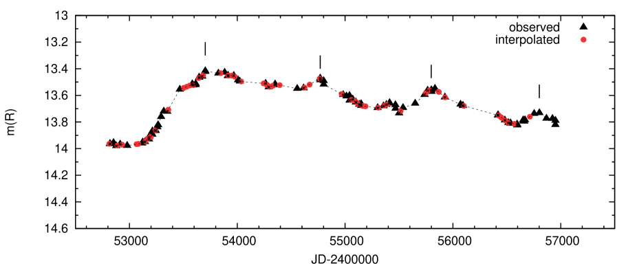
Figure 1: R-band light curve for observed and interpolated data. The four maxima are denoted on the plot. The error bars are comparable to the symbol size.

The photometry in BVR filters of E1821+643 was performed at the Special Astrophysical Observatory of the Russian Academy of Science (SAO RAS) during the 2003–2014 period (98 nights) with the 1m Zeiss telescope with an offset guided automatic photometer. The photometer contains a CCD camera of the size of 1040$\times$1160 pixels, that is cooled with liquid nitrogen (Amirkhanian et al., 2000). The pixel scale at the CCD is 0.45″/pixel, that correspons to 7.5$\times$8.5 arcmin field of view. Both bias and dark current frames were taken, while for the flat-filed frames we adopted the morning and evening sky exposures. The software developed at SAO RAS by Vlasyuk (1993) was used for the data reduction. The photometry is done by integrating the signal in the concentric circular apertures of increasing size, that are centered at the baricenter of the measured object. The photometric system of this instrument resemble those of Johnson in B and V filter, and of Cousins in R filter (Cousins, 1976). For local photometric standards we used stars of Penston et al. (1971) that are close to the position of E1821+643 on our CCD images, which results with the negligible effects of differential air mass. In Table 1 (available electronically only) the photometric BVR-magnitude for the aperture of 15″are presented and in Fig. 1 we plotted the light curve in the R-band.

2.2 Spectral observations

Spectra of E1821+643 ($\sim$140 nights) were acquired with two telescopes (6 m and 1 m) of the SAO RAS, Russia (during 1998–2014), one telescope (INAOE’s 2.1 m) of the Guillermo Haro Observatory (GHO) Cananea, Sonora, México (during 1998–2007, and 2013), and two telescopes (3.5 m and 2.2 m) of Calar Alto Observatory (CAO), Spain (during 1990–1994). All spectra were acquired with long-slit spectrographs with CCDs. The representative wavelength interval was from 4000 Å to 7500 Å, with the spectral resolution between 4.5 Å and 15 Å, and the S/N ratio $>$50 in the continuum close to the H$\beta$ line. Every night the spectrophotometric standard stars were observed. Information on the source of spectral observations is listed in Table 2, while the log of spectral observations is listed in Table 3 (available electronically only).

The spectrophotometric data reduction was performed using the software developed at SAO RAS, while for the spectra acquired in Mexico and in Spain the IRAF package was used. The image reduction procedure consisted from the standard bias and flat-field corrections, cosmic ray removal, 2D wavelength linearization, sky spectrum subtraction, addition of the spectra for every night, and relative flux calibration based on standard star. Further in the analysis, we rejected approximately 10% of spectra due to different reasons (e.g. poor spectral resolution ($>$15 Å), high noise level, badly corrected spectral sensitivity, etc.), thus our final data set contains 127 spectra, that are further analyzed.

2.3 Absolute calibration (scaling) of the spectra

The common technique of the spectral flux calibration based on the comparison with stars of determined spectral energy distribution, is not precise enough for the study of an AGN variability, as the spectrophotometric accuracy is not less than 10% even under great photometric conditions. Thus the standard stars were only used for a relative flux calibration. For the absolute calibration, the AGN narrow emission lines fluxes were used for scaling the spectra, because it is noted that these lines do not vary on time scales of decades (Peterson, 1993).

E1821+643 is a QSO with very bright [OIII] $\lambda\lambda$4959,5007 emission lines and it is possible to scale our spectra using the flux of these lines. However, a problem may be that the [OIII] lines are varying during the long monitored period of 24 years.

The very bright [OIII] emission (two orders of magnitude brighter than in other radio-quit quasars, see Fried, 1998) indicates the presence of a very large narrow line region (NLR). Taking the relation $R_{\rm NLR}\sim L[{\rm OIII}]^{0.33}$ given by Schmitt et al. (2003) and the [OIII]$\lambda\lambda$4959, 5007 flux of the order of $\sim 2\times 10^{-13}\rm{erg\,cm^{-2}s^{-1}}$ for E1821+643 (z$\approx 0.3$), we estimated that the size of the extended NLR is of the order of $\sim$8 kpc (26000 light years), that is three orders of magnitude larger than our monitored period (24 years), consequently one cannot expect to detect the variability in the [OIII] line flux during this monitored period.

Therefore, we used the [OIII]4959+5007 integrated line flux, that is taken to be $2.9\times 10^{-13}\rm{erg\,cm^{-2}s^{-1}}$ (Kolman et al., 1993), in order to absolutely calibrate our spectra with the method proposed by van Groningen & Wanders (1992) that is modified by Shapovalova et al. (2004). Note that this method was tested for different S/N$>$20 and different spectral resolutions, and it has been shown that the uncertainty in the scaling is $\sim$1-2%, and depends only on the quality of the spectra. For more details see van Groningen & Wanders (1992) and Appendix A in Shapovalova et al. (2004).

2.4 Unification of the spectral data

For the study of the long term spectral variability of an AGN observed with telescopes of different apertures, it is mandatory to construct an uniformed data set in a consistent way. Since instruments of different apertures were used for the observations, it is necessary to correct for aperture effects both the continuum and line fluxes (Peterson & Collins, 1983). Based on our past work (Shapovalova et al., 2001, 2004, 2010, 2012, 2013), we determined a point-source scale correction factor ($\varphi$) and an aperture-dependent correction factor that corrects for the host galaxy contribution to the continuum, i.e. extended-source correction factor (G(g)). We used the following expressions (see Peterson et al. (1995)):

$$F({\rm line}){\rm true}=\varphi*F({\rm line}){\rm obs},$$

$$F({\rm cont}){\rm true}=\varphi*F({\rm cont}){\rm obs}-G(g),$$

where index ”obs” denotes the observed flux, and ”true” the aperture corrected flux. The spectra of the 6m telescope, within an aperture of 2″$\times$ 6″were adopted as standard (i.e. $\varphi$= 1.0, G(g)=0 by definition). The correction factors $\varphi$ and G(g) are estimated empirically, comparing the observations from all telescope data sets with the simultaneous one from the standard data set (the same method was used in AGN Watch, see e.g. Peterson et al. (1994, 1998, 2002)). Intervals which we noted as ”nearly simultaneous” are practically of 1-3 days, suppressing the variability on short time scales ($<$ 3 days). The point-source scale correction factor $\varphi$ and extended-source correction factor G(g) values (in units of 10${}^{-15}\rm erg\,cm^{-2}s^{-1}\AA^{-1}$) are given for different data sets in Table 4.

2.5 Measurements of the spectral fluxes and errors

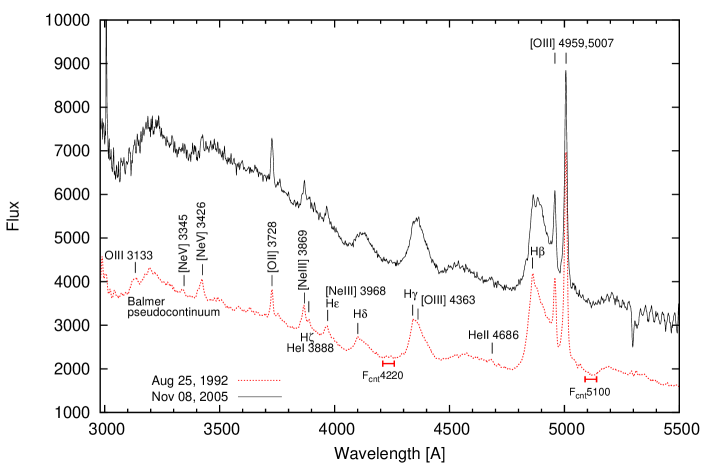
Figure 2: Example of two E1821+643 rest-frame spectra observed close to the minimum (down) and maximum (up) of activity in the monitoring period. The observed lines and continuum windows are denoted on the plot.

From the scaled spectra (see sections 2.2–2.3) we measured the continuum flux near the H$\beta$ line at the observed wavelengths $\sim 6616$ Å  ($\sim 5100$ Å  in the rest frame), by averaging fluxes in the spectral range of 6601–6631 Å  and the continuum flux near the H$\gamma$ line at the observed wavelengths $\sim 5474$ Å  ($\sim 4220$ Å  in the rest frame), by averaging fluxes in the spectral range of 5459–5489 Å. Note that the spectrum of E1821+643 does not contain significant absorption lines in the observed spectral range (see Fig. 2).

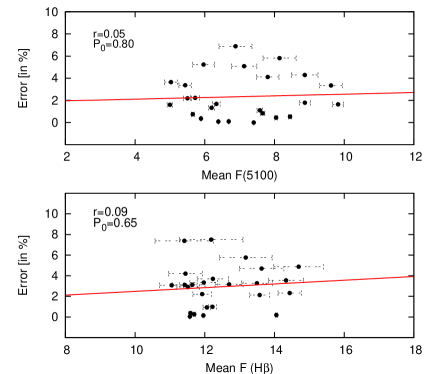
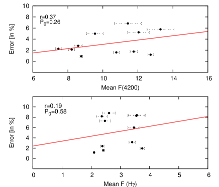
Figure 3: The H$\beta$ line and continuum at 5100 Å  flux errors (left panels), and H$\gamma$ line and continuum at 4200 Å  flux errors (right panels) with respect to the corresponding mean flux. The continuum flux is in units of 10^-15 erg cm^-2s^-1Å^-1, and the line fluxes are in units of 10^-13 erg cm^-2s^-1.

For the determination of the H$\beta$ and H$\gamma$ fluxes, we must first subtract the underlying continuum. For this goal, a linear continuum was fitted through the windows of 20 Å , 6160–6635 Å  for the H$\beta$ region, and 5480–5780 Å  for the H$\gamma$ region. Then, the observed line fluxes were measured in the following wavelength intervals: (6170–6620) Å  for H$\beta$ and (5550–5770) Å  for H$\gamma$. Using $\varphi$ and G(g) factors from Table 4, we re-calibrated the observed H$\gamma$ and H$\beta$ fluxes, and their corresponding near-by continuum fluxes to a common scale using the standard aperture of 2.0″$\times$6.0″. In Table 5 (available electronically only) the fluxes for the continuum at the rest frame wavelength of 5100 Å  and 4220 Å, the total H$\gamma$ and H$\beta$ lines, and their errors are given. The listed total H$\gamma$ and H$\beta$ fluxes include the contribution of the narrow H$\gamma$ and H$\beta$ component and the [OIII] 4363, 4959, 5007 lines. The mean errors (uncertainties) of the continuum fluxes at 5100 Å  and 4220 Å  H$\beta$, and H$\gamma$ lines are $\sim$(2-3.5)%, $\sim$3.5%, and $\sim$5%, respectively (see Table 6). These quantities were estimated by comparing results from spectra obtained within a time interval shorter than 3 days. Note that the errors in fluxes in Table 5 were obtained using the mean error from Table 6. Figure 3 shows mean errors in the flux measurements as function of the corresponding mean line fluxes for H$\beta$ and H$\gamma$, and for the continuum at 5100Å  and 4220Å. The correlation coefficient and corresponding p-value are also given in Figure 3. As can be seen it is obvious that the dependence between the mean error and the mean fluxes does not exist between F(H$\beta$) and F(5100), or have a very weak trend (statistically insignificant) between F(H$\gamma$) and F(4200).

The contribution of the host galaxy can be very important in some objects (see e.g. Shapovalova et al., 2013), especially if the stellar absorption lines are present in the AGN spectrum. Therefore we roughly estimated the contribution of the host galaxy from the aperture photometry with apertures 10″and 15″. One can expect that in the ring between 15″and 10″, the flux in V and R filters is from the host galaxy, therefore we used the ratio of the ring flux to the 10″-aperture flux to estimate the host-galaxy contribution. We obtained that the contribution of the host galaxy in the V-band is from 3.0% to 4.6%, relative to the flux in the maximum and minimum activity states of the nucleus, respectively. In the R-band the host galaxy contribution is from $\sim$3% to 9%. This is not in contradiction with an estimate made in the V-band by Floyd et al. (2004) from the modeling of an HST/WFPC2 image of this object. They found that the host-galaxy contributes around $\sim$10% to the total luminosity in the V-band in 2000 (when the object was close to the minimum state). Also, we should note that in the spectra of E1821+643 the stellar absorption lines such as Mg Ib (5170), Ca II (H,K), and G-band (4302) are absent, which indicates a very small host-galaxy contribution.

2.6 The broad H$\beta$ line and its segment fluxes

In this paper we will extract only the broad component of the H$\beta$ line and study the behavior of its line segments during the monitored period. The detailed analysis of the H$\beta$ and H$\gamma$ line profiles using the Gaussian-fitting method will be given in the forthcoming paper (Paper II).

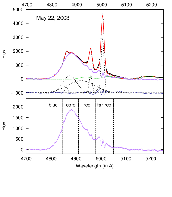
Figure 4: Upper: Example of the best Gaussian fit of the continuum-subtracted spectrum around the H$\beta$ spectral region (observed on May 22, 2003). Below the observed spectrum (dots), the best-fit (thick solid line), and the Fe II template (dashed line) are given. The residual (thin solid line), and the Gaussian broad and narrow components (dashed line) are shifted below for better visibility. Bottom: Broad H$\beta$ component, after subtraction of narrow lines and Fe II lines. The segments (blue, core, red and far-red) of the line are separated by vertical lines.

To obtain only the broad component of the H$\beta$ line we subtracted the underlying continuum that was fitted through the continuum windows using the B-spline python routine interpolate.splev. Then we applied an automatic and self-consistent multi-Gaussian fitting method for removing the narrow components of H$\beta$, [OIII]$\lambda\lambda$4959,5007Å  lines, and Fe II lines (Popović et al., 2004; Kovačević et al., 2010; Shapovalova et al., 2012) The fitting-method is based on the $\chi^{2}$-minimalization routine, and we reduced as many Gaussian parameters as possible: i) all narrow lines have the same widths and shifts (see Popović et al., 2004); ii) the flux ratio of [OIII]$\lambda$4959Å  and [OIII]$\lambda$5007Å  is 1:3 (Dimitrijević et al., 2007); iii) two broad Gaussian functions (broad and very broad line component) were used to fit the broad H$\beta$ component; iv) the ionized iron line multiplets have lines of same widths and shifts (Kovačević et al., 2010; Shapovalova et al., 2012). One example of the best fit (thick solid line) of the observed spectrum (dots) is presented in upper panel of Figure 4, where the 42 Fe II multiplet (dashed line) is also shown. The residual (thin solid line), and the Gaussian broad and narrow components (dashed lines) are shifted below for better visibility (Fig. 4). Note here that only one Gaussian cannot properly fit the narrow line wings of strong [OIII] lines, therefore, we included an additional, broader, Gaussian (with significantly smaller intensity) to fit the narrow [OIII] lines wings.

We determined the flux of the broad H$\beta$ component in the same wavelength range as for the total H$\beta$ line and estimated that the contribution of the narrow components is $\sim$30%. We also found that the peak of the broad H$\beta$ component is shifted by $\sim$1000 km s^-1 relative to the peak of the narrow component. Measuring the flux of the broad H$\beta$ line-segments we divided the broad H$\beta$ component relative to the shifted center (4877.5 Å, in the rest-frame) into four line-segments with the width of $\sim$4000 km s^-1 each: blue wing, core, red wing, and far red wing (see the bottom panel in Figure 4 and Table 6). Then we determined the fluxes of these line-segments (Table 7, available electronically only). The mean errors for the broad H$\beta$ line-segment fluxes are about 3%-6% (Table 6). As expected, the maximal error $\sim$6% corresponds to the distant, far-red wing and is caused by a bad subtraction of the bright [OIII]$\lambda$5007Å  line, and a weak line intensity in this spectral region. The mean errors (in %) of fluxes and the line-segment fluxes are given in Table 6 and in Table 7 (available electronically only), respectively.

3 Data analysis and results

3.1 Photometric results

In Table 1 the results of the broad-band photometry of E1821+643 in BVR filters for a circular aperture of 15″and the corresponding errors are listed. A light curve in the R-band shows an almost sinusoidal change with the maximum amplitude of about 0.5 magnitude (see Figure 1). There, we can see several ($\sim$4) noticeable peaks (flares, outburst) with different brightness amplitudes. In the BV-bands the light curves have the same shape. Some information about these flare-like events are listed in Table 8. It follows that the amplitude of peaks varies from 0.1 to 0.54 magnitude, or in intensity from 1.1 to 1.6 times. It is very interesting to note that the difference in days between the two consecutive flare-like events is $\sim$1000 days (Table 8). This indicates some periodicity in the flux variability during the monitored period. Further (in section 3.2.4) we study the periodicity of light curves using different methods.

3.2 Spectral results

Figure 2 shows typical spectra of E1821+643 observed close to the minimum and maximum activity during the monitored period. It is obvious that in the spectra of E1821+643 the broad emission lines of the hydrogen Balmer series and the big blue bump are most outstanding. Also the narrow components of the Balmer lines and various forbidden lines, typical for AGN (the most prominent [OIII]4959+5007 lines) are observed. As can be seen in Figure 2, there is no dramatic change in the spectral energy distribution and Balmer continuum between the minimum and maximum stages. Using the narrow line components we obtained the average redshift of $z=0.2972\pm 0.0002$ which we take as the rest frame of the host galaxy. We confirmed, as other authors found as well (see Landt et al., 2008; Robinson et al., 2010, etc), that the peaks of the broad Balmer line components are red shifted with respect to the narrow line components by $\sim$1000 km s^-1. The broad Balmer lines have extremely asymmetric profiles, with red wings extending to Doppler velocities of at least $\sim$15000 km s^-1 relative to the rest frame wavelength (Table 6).

3.2.1 Variability of the emission lines and the optical continuum

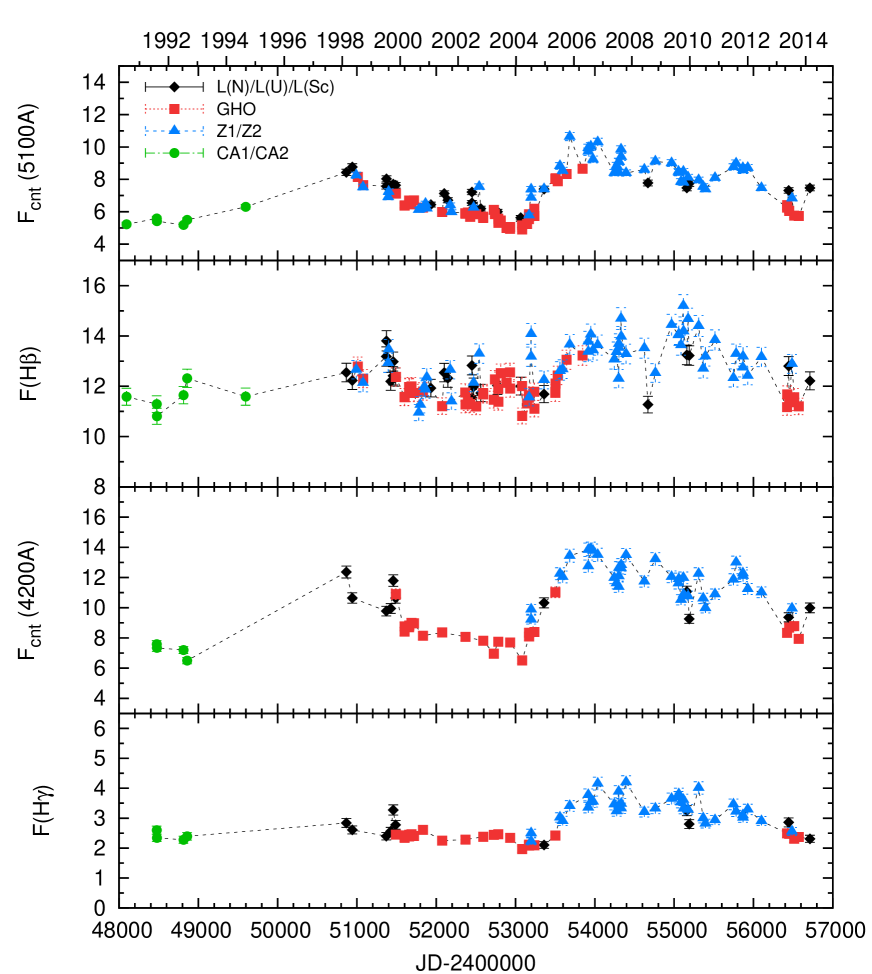
Figure 5: Light curves (from top to bottom) for the continuum at 5100Å, total H$\beta$, continuum at 4200Å, and total H$\gamma$ line fluxes. Observations with different telescopes are denoted with different symbols given in the upper plot. The continuum flux is in units of 10^-15 erg cm^-2s^-1Å^-1, and the line flux in units of 10^-13 erg cm^-2s^-1.

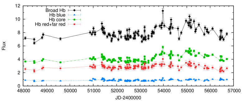
Figure 6: Light curves of the broad-component and line-segment fluxes of H$\beta$. The fluxes are in units of 10^-13 erg cm^-2s^-1.

We analyzed flux variations in the continuum and lines using a total of 127 and 76 spectra covering the H$\beta$ and H$\gamma$ wavelength regions, respectively. In Table 5 fluxes in continua at 5100 Å  and 4200 Å, and total H$\beta$ and H$\gamma$ lines are listed. Using these data we plotted the light curves for the continuum at the rest wavelengths 5100 Å  and 4200 Å, and for the H$\beta$ and H$\gamma$ lines (see Figure 5). It is obvious that the fluxes in the continua and lines are varying during this monitored period (1990–2014). In the continuum light curves, and with some possible delay in the H$\beta$ and H$\gamma$ light curves, the same flare-like events (1-3 from Table 8) as in the R-band photometric light curve (see Figure 1) are seen. In Figure 6 the light curves for the broad H$\beta$ line component and its different line-segments are given. Both fluxes in the broad H$\beta$ line component and in its line-segments (blue, core, red+far red, Table 7) vary quasi-simultaneously and local maxima, approximately close to the flare-like events 1-3, are also traced. In Figure 6, there are some indications of the presence of the shorter time-scale fluctuations (flares) in the light curves of the total-line and line-segment fluxes. These flare-like features become clearer in the artificially generated light curves (see Section 4.1). One can suspect that a fraction of short-time flares arise from the uncertainties in the relative flux calibration (i.e. unification of the spectral data, see Sections 2.4 and 2.5), however, the short-time flares can be also detected in spectrophotometic curves as a consequence of short time variability of the nucleus. For example, in several other objects, the short-time flares have been registered in line/continuum light curves (e.g. Ark 564 and Arp 102B, see Shapovalova et al., 2012, 2013). Since in case of this object, the short-time flares are not within the frame of the error-bars, thus it seems that from time to time the short-time flare events are present in the light curves of E1821+643.

For the variability estimates of the line and continuum fluxes, we used the method given by O’Brien et al. (1998). In Table 9 we give parameters that describe the variability of the continuum and total line fluxes, i.e. N is the number of spectra, $F$ denotes the mean flux over the whole observing period, and $\sigma(F)$ is the standard deviation, and $R$(max/min) is the ratio of the maximal to minimal flux in the monitoring period. The parameter $F$(var) is an inferred (uncertainty-corrected) estimate of the variation amplitude with respect to the mean flux, defined as:

$$F({\rm var})=[\sqrt{\sigma(F)^{2}-e^{2}}]/F({\rm mean})$$

$e^{2}$ being the mean square value of the individual measurement uncertainties for N observations, i.e. $e^{2}=\frac{1}{N}\sum_{i}^{N}e(i)^{2}$ (O’Brien et al., 1998). From Table 9 it follows that the fluxes in the continuum (at rest 5100 Å  and 4200 Å) and total H$\gamma$ line changed for about 2 times, while in the H$\beta$ flux only for $\sim$1.4 times. The difference in the line flux variations between H$\beta$ and H$\gamma$ may be caused by different dimensions of emitting region for these two lines (i.e. H$\gamma$ emitting region is significantly smaller than H$\beta$ one). In addition, the smaller variability in the H$\beta$ flux may be caused by the contribution of the constant fluxes from narrow lines [OIII]4949,5007. The amplitude of variability F(var) is $\sim$19% for the continuum and total H$\gamma$ line, and $\sim$7% for the total H$\beta$ line. The fluxes of the broad H$\beta$ segments (blue, red, far-red wings, and core) vary quasi-simultaneously with F(var)$\sim$11-12% (Table 9, Fig. 6).

3.2.2 The lines and continuum flux correlations

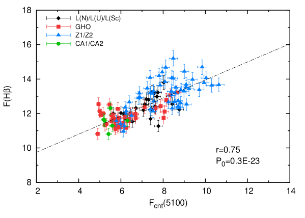
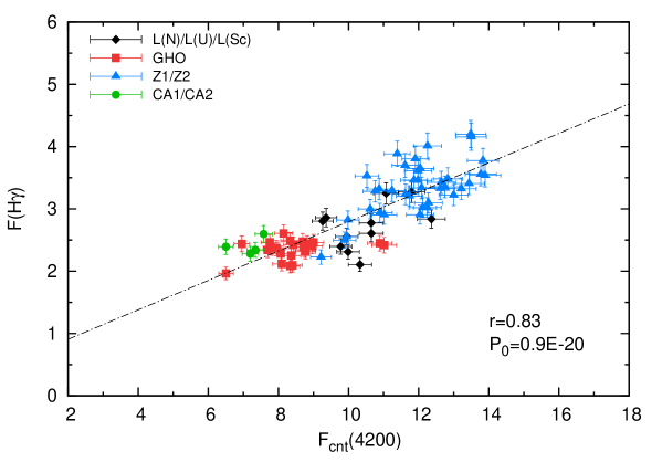
Figure 7: H$\beta$ vs continuum at 5100Å  flux (upper) and H$\gamma$ vs. continuum at 4200Å flux (bottom). The continuum flux is in units of $10^{-15}\rm erg\ cm^{-2}s^{-1}\AA^{-1}$, and the line flux in units of $10^{-13}\rm erg\ cm^{-2}s^{-1}$. Observations with different telescopes are denoted with different symbols given in the upper left. The correlation coefficients and the corresponding p-values are also given.

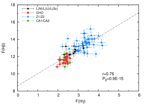
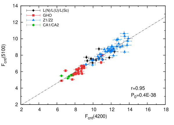
Figure 8: The H$\beta$ vs. H$\gamma$ flux (upper) and continua 5100Å vs. 4200Å flux (bottom). The continuum flux is in units of $10^{-15}\rm erg\ cm^{-2}s^{-1}\AA^{-1}$, and the line flux in units of $10^{-13}\rm erg\ cm^{-2}s^{-1}$. Observations with different telescopes are denoted with different symbols given in the upper left. The correlation coefficients and the corresponding p-values are also given.

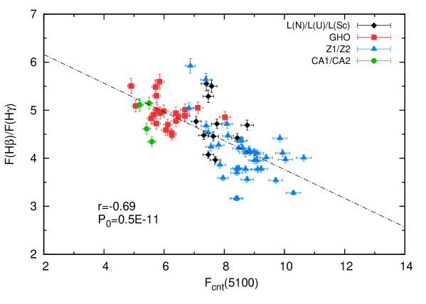
Figure 9: H$\beta$/H$\gamma$ flux ratio vs. continuum flux at 5100Å. The continuum flux is in units of $10^{-15}\rm erg\ cm^{-2}s^{-1}\AA^{-1}$. Observations with different telescopes are denoted with different symbols given in the upper right. The correlation coefficients and the corresponding p-values are also given.

Figure 7 shows the relationship between the total line (H$\beta$, H$\gamma$) and the adjacent continuum fluxes (at 5100 Å  for H$\beta$ and 4200 Å  for H$\gamma$). The correlation coefficients in both cases are quite high ($\sim$0.8), indicating that the ionizing continuum is a good extrapolation of the optical continuum. We should note here that there is a slightly better correlation between the flux of H$\gamma$ and the continuum at 4200 Å  than between H$\beta$ and continuum flux at 5100 Å. This indicates a faster response of the H$\gamma$ line flux to the corresponding continuum changes, than seen in H$\beta$. In Figure 8 the relationship between H$\beta$ and H$\gamma$ fluxes (upper panel) and between the continua at 4200 Å  and 5100 Å (bottom panel) are given. As can be seen, there are good correlations between the ratio of the H$\beta$ and H$\gamma$ total line fluxes (r$\sim$0.76), and even better between two continua (r=0.95). Figure 9 gives the correlation between the total line-flux ratio H$\beta$/H$\gamma$ vs. continuum flux at 5100 Å. A strong anti-correlation (r$\sim$0.7) is observed in this case. This also indicates faster and stronger reaction of the H$\gamma$ line flux to the continuum than the H$\beta$ one. Finally, in Figures 10 and 11 the correlations between the broad H$\beta$ line, its line-segments and continuum flux, as well as correlations between different broad line H$\beta$ line-segments relative to each others are given. There are significant correlations (r=0.6-0.8) between the line core and red wing flux with the continuum flux, however the correlation of the blue wing and continuum fluxes is smaller (r=0.35) and less statistically significant.

3.2.3 Time-lag analysis

There are several classes of methods for handling the problem of irregular data sets time-lag analysis. Perhaps the oldest class of estimators is standard interpolation (using linear and cubic-spline) of observations in order to create time series on a regularly spaced grid. This method leads to significant reduction in variance toward the high-frequency range of the estimated power spectrum. When there are interests in phenomena on smaller timescales (relative to the mean sampling interval) such effects should be taken into account. Beside this, the persistence (memory) of irregularly time series is strongly overestimated when using the standard (linear and cubic spline) interpolation approach (Rehfeld et al., 2011).

Our data sets are irregular, thus for the time-lag analysis of the spectroscopic and photometric light curves we applied three methods: (i) the Discrete Correlation Function (DCF; Edelson & Krolik, 1988), (ii) the z-transformed Discrete Correlation Function (ZDCF; Alexander, 1997, 2013), both methods from the class of slotting time-lag estimators, and (iii) the Stochastic Process Estimation for AGN Reverberation (SPEAR) by Zu et al. (2011), recently developed method that is a model-based estimator that uses a damped random walk model (DRW model Kelly et al., 2009; Kozlowski et al., 2010; McLeod et al., 2010). For more details on all three methods and their differences and advantages see a recent paper by Kovačević et al. (2014, and references therein).

We calculated the DCF and ZDCF functions over the major time range of our monitoring campaign (the points before 1998 are excluded due to extremely poor sampling). The ZDCF lags are taken to be the peaks of the CCFs, while the uncertainties are addressed using the Monte Carlo method (Alexander, 1997, 2013). The DCF lags, DCF coefficients and their errors are calculated using the MATLAB bootstrap toolbox for time series analysis. For this, we constructed 1000 clones of our light curves. Each clone is made by choosing random samples with replacement from mother curve, i.e. each observation is selected separately at random from the original dataset. The number of elements in each bootstrap clone equals the number of elements in the original data set. Then the centroid of DCF was computed for each pair of clones so we can construct bootstrap vectorial statistics of time lags and centroid of DCF. The mean values are chosen as the final DCF lag and coefficients results, and the uncertainties are calculated as standard deviations of their bootstrap distributions.

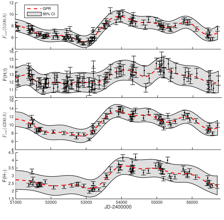
Figure 12: Comparison between the GPR generated (dashed line) and observed light curves (circles with errorbars) of the continuum at 5100Å, H$\beta$, the continuum at 4200Å, and H$\gamma$ (from top to bottom). The shaded band represents $95\%$ confidence interval (CI) for the GPR predicted curve.

Since our light curves have large mean sampling, we attempt to probe time-lags of artificial time series with better sampling and which points are ”predictions” obtained from original time series. For this task we employed Gaussian process regression (GPR) for noisy data (Rasmussen & Williams, 2006). GPR generates data such that if we observe their values, they would follow a multivariate Gaussian distribution. The main constituents of a GPR are its covariance and mean functions. With covariance function we encode correlations (relations or similarities) between different data points in the process. We specified a GPR for our artificial time series as follows: a constant mean function, with initial parameter set to mean of original time series, and an isotropic squared exponential covariance (kernel) function. The covariance function takes two hyperparameters, a characteristic length-scale and the standard deviation of the original signal. The length-scale was set to 150. Fig. 12 gives the comparison between the GPR generated and observed light curves of the continuum at 5100Å, H$\beta$, the continuum at 4200Å, and H$\gamma$ (from top to bottom).

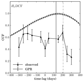
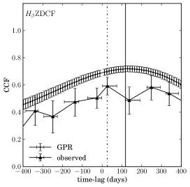
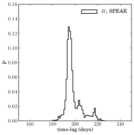
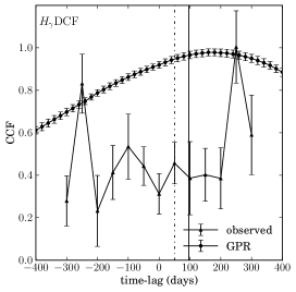
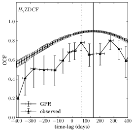
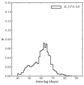
Figure 13: The derived CCFs of the observed (triangles) H$\beta$ (upper panels) and H$\gamma$ (bottom panels) time-lags from the DCF (left) and ZDCF (middle) methods, and the equivalent probability distribution P from the SPEAR method (right). The solid continuos curves give for comparison the derived CCFs of the corresponding GPR generated artificial light curve. The vertical lines denote the obtained time-lag in case of the observed (dash-dotted) and GPR generated (solid) data.

Table 10 summarizes the results of all three time-lag estimators we employed on both observed and GPR generated artificial light curves of H$\beta$ and H$\gamma$ and the corresponding continuum light curves. The GPR artificial light curves have uniform and better sampling. Fig. 13 gives the derived CCFs (triangles) of H$\beta$ (upper panels) and H$\gamma$ (bottom panels) time-lags from the DCF (left panels) and ZDCF (middle panels) methods, and the equivalent probability distribution from the SPEAR method (right panels). The derived CCFs of the corresponding GPR generated artificial light curve are also given for comparison. The large number of points in the GPR light curves leads to better constrained uncertainties in the case of the DCF and ZDCF methods, due to consequently larger number of binned points.

In case of the DCF and ZDCF methods, the derived CCFs obtained from the observed light curves (left and middle panels in Fig. 13) typically contain two peaks of similar amplitude that (considering the error bars) are not statistically distinguishable. In Table 10 we listed the values of the first clearly visible peak. With this we demonstrated that the reliable lags cannot be recovered directly from this data sets using the DCF and ZDCF methods. Another point that can be seen from Table 10 is that the ZDCF gives for both H$\beta$ and H$\gamma$ the time-lags that are similar to the median sampling interval, and thus might be considered as spurious. However, this may also be a coincidence as other authors have obtained time-lags similar to the median sampling interval (see e.g. Denney et al., 2009).

Also we should note here, that the obtained time-lags can be influenced by the relative flux calibration (i.e. unification of the spectral data, see Sections 2.4 and 2.5) of the spectra and the short-time flares, which can be seen in the light curves of the continua and broad lines. Data calibration procedure in constructing the light curves can affect the traditional CCFs analysis, and can have greater effect on the lag analysis of the more sparsely sampled H$\gamma$ – continuum light curves. That is why we additionally applied the SPEAR method, which has been tested for different calibration effects, and it has been shown that the impact on the estimated lag is generally negligible (see Zu et al., 2011). Additionally, as can be seen in Fig. 12, the GPR procedure allows us to avoid the influence of the flare-like local peaks.

The SPEAR method treats large time-gaps in light curves in a statistically based approach, and considers the impact on the uncertainties of the time-lag. Our data sets have large time-gaps in the light curves and flare-like peaks, thus the obtained ZDCF and DCF curves are degenerated, while the SPEAR time-lag probability distributions are well defined with no deterioration. Therefore the obtained SPEAR lags are preferred.

As a summary of our CCF analysis, we can state that there is a large difference between the H$\beta$ and H$\gamma$ lags obtained from the SPEAR method (in both cases, for the observed and GPR time-series). It seems that the H$\gamma$ emitting region is smaller than the H$\beta$ one, that is also in agreement with dependence of the flux ratio of lines as a function of the continuum (see Figure 9). Further in the text, we will use the values of lags obtained from the SPEAR method applied on the GPR generated artificial light curves, i.e. the lag for H$\beta$ $\sim 120$ and for H$\gamma$ $\sim 60$ days.

3.2.4 Periodicity

As noted in sections 3.1 and 3.2.1, 3-4 maxima are visible in the photometric and spectral light curves (see Figure 1, the maxima are denoted with vertical ticks). This motivated us to search for periodicities in different light curves.

We applied periodogram analysis to test whether our time series contain only noise or some periodic components are present. In the case of presence of semi-periodic or even non-periodic components, the periodogram can show more than one prominent peak. Another problem is that the mean values are not always good estimator of the mean of periodogram underlying function, causing problems as aliasing. In order to avoid these problems, we applied several techniques to our time series: (i) ”Generalized” Lomb-Scargle periodogram(GLS Lomb, 1976; Scargle, 1982), (ii) multiterm periodogram routine (MP Vanderplas et al., 2012; Ivezić et al., 2014), and (iii) Bayesian Generalized Lomb-Scargle periodogram (BGLS Mortier et al., 2015). GLS treats the problem of the mean overestimation by adding constant offset term to the model. MP treats the problem if the data have hidden variability that is more complex than single sinusoidal. BGLS includes both weights and a constant offset in the data.

Figure 14 compares GLS of our time series. The light curves of continua at 4200 Å and 5100 Å, and the H$\beta$ and H$\gamma$ lines have a strong peak corresponding to the period of about 4500 days, that is the only statistically significant peak. Periodograms of both H$\beta$ and H$\gamma$ lines show another two peaks around 1300 days and 780 days ($\omega\in[0.003,0.005]$), but they are bellow the 1% and 5% significance levels. The peak of about 780 days ($\sim$ 2 years) can be a consequence of observation conditions. MP and BGLS techniques give a peak that is also about 4500 days for both continuum and both line light curves. Periodograms of fluxes of photometric curves show 3 prominent and statistically significant peaks around 4000, 1850, and 1200 days (Figure 14).

Comparing the obtained periods with observed peaks in light curve, one can see that the 4000 (photometric) and 4500 (spectroscopic) day periods are representing only one cycle period and it is hard to conclude that we found a good evidence for periodic behavior with approx. 4000 day period. However, the 1200 day period, that is associated with the 4 flare-like events in the photometric light curve represents an evidence for a periodic variability in the photometric light curve, as well as in the spectroscopic light curves (1300 days, even it has a small significance level). The period of 1850 days found in the photometric light curve, is not present in the spectroscopic light curves. With current analysis of the variability in the continuum and line fluxes we cannot find any associated physical phenomena with this period.

The mean sampling period of the continuum and light curves is about 50 days, so it is possible that any shorter period is hidden in the poor data sampling since MP and BGLS could not retrieve them with larger significance.

3.2.5 Line profile variation

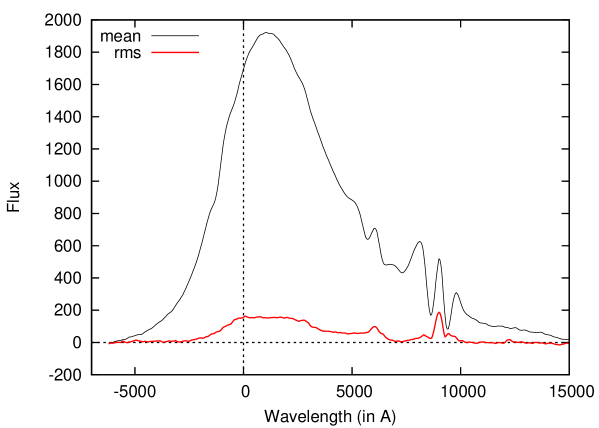
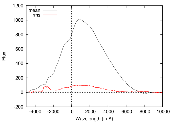
Figure 15: Mean and rms spectra of the broad H$\beta$ (upper) and H$\gamma$ lines (bottom).

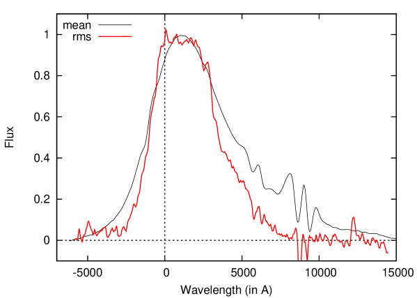
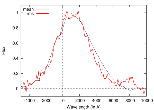
Figure 16: The comparison of mean and rms spectra of the broad H$\beta$ (upper) and H$\gamma$ (bottom).

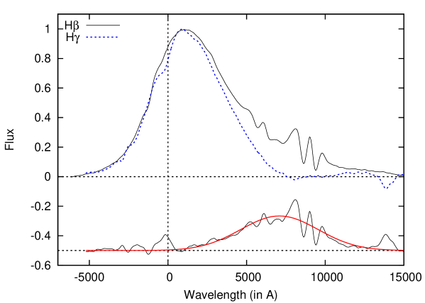
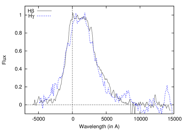
Figure 17: The comparison of the mean broad H$\beta$ and H$\gamma$ profiles (upper) and their rms (bottom). The difference between the H$\beta$ and H$\gamma$ mean profiles is also given at the bottom of the upper plot, fitted with a single Gaussian.

Using the continuum and narrow line subtracted spectra, we constructed the mean and root-mean-square (rms) line profiles of the broad H$\beta$ and H$\gamma$ components (see Figure 15), which shows that the broad lines have negligible changes in their profiles, i.e. during a long period of 24 years the H$\gamma$ and H$\beta$ line profiles have a strong red asymmetry, and peaks of both lines are red shifted for about 1000 km s^-1. We measured the full width half maximum (FWHM) of H$\beta$ of 5610 km s^-1, which is larger than the FWHM of H$\gamma$ (5060 km s^-1), while the FWHM of rms profile of H$\gamma$ (4740 km s^-1) is only slightly higher than H$\beta$ one (4520 km s^-1). In Figure 16 we compare the mean and rms profiles of H$\gamma$ and H$\beta$ lines. The residuals of the narrow lines subtraction have been artificially corrected in the rms profiles for better comparison. As it can be seen in Figure 16, the rms profile of H$\beta$ shows smaller changes in the blue wing, and in the red part of the line, while the rms of H$\gamma$ shows smaller variability in the far red wing. We compare the mean H$\gamma$ and H$\beta$ profiles (upper panel) and their rms (bottom panel) in Figure 17. It is interesting that the rms profiles seem to be the same, while, the mean H$\beta$ has more extensive red wing than the mean H$\gamma$. It seems that there is an additional emission in the far wing of the mean H$\beta$, which is clearly seen when the two mean profiles are subtracted (Figure 17, upper panel). We fitted a simple Gaussian through the difference of the mean spectra, that is shifted to 7090 km s^-1 and with a FWHM of 5810 km s^-1. We measured that the ratio of the red to the blue part of FWHM is 3.8 for the mean H$\beta$ and 3.1 for the mean H$\gamma$, that confirmed the observed difference in the asymmetry of the mean profiles.

4 Discussion

We have presented and analyzed the photometric and spectral data for QSO E1821+643 obtained from the long-term monitoring (2003–2014 for photometry; 1990–2014 for spectroscopy). Here we discuss the obtained results.

4.1 Variation in the continuum and broad lines

The results of the multi-wavelength monitoring of E1821+643 in X-ray, UV and optical ranges, simultaneously observed for 37 days, were reported in Ulrich et al. (1992). They found that there are no short-term changes in the UV and optical spectra, while in the X-ray, there exists a variability on the short term scale. This result has been confirmed by Kolman et al. (1993), they also found possible changes on the larger time scale in the UV/optical spectra. Here, we explore the variability of E1821+643 in the 24-year period in the continua at 4200Å  and 5100 Å, and in the broad H$\gamma$ and H$\beta$ emission lines. We find significant changes in the line and continuum fluxes during the monitored period. It is interesting that the H$\gamma$ line flux has changed for about two times (similar to continua at 4200 and 5100 Å), while the H$\beta$ line showed smaller variations in the line flux (1.4 times). We found that variations of both lines well correlate with variations of the corresponding continuum, but the response of the H$\gamma$ line is better than of the H$\beta$ line. This, and also the CCF analysis, indicates that the emitting region of the H$\beta$ line is distinctly larger than the emitting region of the H$\gamma$ line. This indicates a possible stratification in the BLR, showing smaller H$\gamma$ emitting region, that is also observed in a number of AGNs (see Table 13 in Bentz et al., 2010). The BLR photoionization models predict a very similar equivalent distribution as a function of ionization parameter and density (Korista et al., 1997), i.e. one cannot expect a significant radial stratification in the broad Balmer lines emission regions. However, the possible radial stratification observed between H$\gamma$ and H$\beta$ emission regions in E1821+643 may be caused by optical-depth effects within the Balmer series (Korista & Goad, 2004). Korista & Goad (2004) showed that there is a modest increase in responsivity between H$\beta$ and H$\gamma$ (see their Table 1). More detailed investigation of this is outside the scope of this paper.

The variability in the H$\beta$ line-segments is present, and it can be seen in Figure 10 that the line core and red wing fluxes are well correlated with the continuum flux at 5100 Å, while a week correlation is present between the blue wing and continuum fluxes.

4.1.1 Periodicity in the variability

First we analyzed the photometric light curves and found flare-like events of different amplitudes (0.1-0.5 magnitude), where the time interval between two consecutive maxima is $\sim$1000 days (see Figure 1 and Table 8). Similar maxima (1–3) are seen in the continuum light curves and possibly, with some delay of $\sim$100 days, in the H$\beta$ and H$\gamma$ line light curves, and in the broad H$\beta$ component and its line-segment light curves (see Figures 5 and 6). We note that it is difficult to detect these maxima in the observed spectroscopic light curves, given the scatter and sampling of data, however, these shorter time-scale fluctuations become clearer in the GPR light curves shown in Figure 12. Since it can indicate the periodical or quasi-periodical changes in the flux, we investigated the light curve periodicities and found in all spectral light curves (in the continua and lines) the significant periodicity with the period of 4500 days. In the photometric light curves, there are three periods of 1200, 1850, and 4000 days. However, as we noted above, the periodicity around 4000–4500 days obtained in spectroscopic and photometric light curves seems to cover only one cycle in our observations and should be confirmed taking a longer observation campaign. These periods in the flux variability can indicate some kind of periodical rotation of some structures (in the disk around SMBH, or some cloudy-like gas) around the central SMBH.

4.2 The SMBH mass and structure of the BLR

The SMBH mass ($M_{BH}$) of E1821+643 can be estimated by using the virial theorem (see Peterson et al., 1998; Wandel et al., 1999):

$$M_{\rm GRAV}=f{\Delta V_{\rm FWHM}\cdot R_{\rm BLR}\over G},$$

where $\Delta V_{\rm FWHM}$ is the orbital velocity at that radius of the BLR, $R_{\rm BLR}$, and it is estimated from the width of the variable part of the H$\beta$ emission line; $f$ is a factor that depends on the geometry of the BLR and can be taken as $f=5.5$ (Onken et al., 2004). Taking into account that the dimension of the H$\beta$ BLR is 120 light days (see Table 10) and that the FWHM of the H$\beta$ rms profile is 4520 km s^-1, we obtained that the central SMBH has a mass of $2.6\times 10^{9}\ M_{\odot}$, which is in agreement with estimates given by Kolman et al. (1993), they found that the mass is $3\times 10^{9}M_{\odot}$.

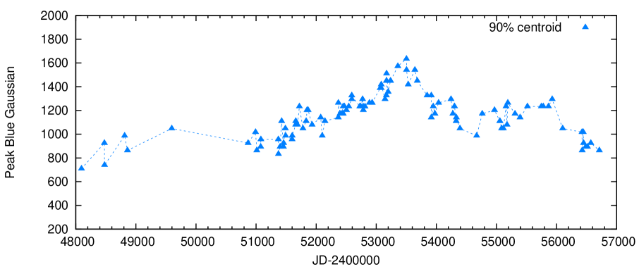
Figure 18: The changes in the redshift of the broad H$\beta$ component during the monitored period, measured as the centroid at 90% of the maximal intensity.

To discuss the structure of the BLR, we should take into account that the broad line profiles have an unusual shape. As we noted in section 2, the broad line profiles have a red asymmetry, i.e. the red wing is two times wider than the blue wing. In addition, the center of the broad H$\beta$ line component is red shifted for $\sim$(1000$\pm$250) km s^-1 relatively to the peak of the narrow component. In the monitored period the peak position of the broad H$\beta$ component is varying from $\sim$700km s^-1 to $\sim$1600 km s^-1 measured as the centroid at 90% of the maximal intensity (see Figure 18). Note here that Landt et al. (2008) reported similar redshifts, of 1000 – 2000 km s^-1 for the broad components of H$\alpha$, H$\beta$ and several Paschen lines, and here we found that this redshift is changing.

It is interesting that the broad H$\beta$ and H$\gamma$ components have different profiles (see Figure 17), with the second one being narrower, since the H$\beta$ has an extended red wing. Additionally, the CCF analysis shows that the H$\gamma$ emitting region is significantly smaller ($\sim 60$ days) than the H$\beta$ emitting region ($\sim 120$ days). However, the shape of the rms of both lines are practically the same (see Fig. 17) that indicates a region which is variable, and that the emission from this region is mostly contributing to the line core of both lines. The far H$\beta$ wing is emitted from another region that shows a smaller variability (see Fig. 17).

Possible shifts of the broad H$\beta$ line peak could be explained with a binary black hole model (Popović, 2012) or with an inflowing BLR (Gaskell, 2009). It is not safe to conclude that an AGN is a supermassive black hole binary system (SMBB) based only on the broad line profiles, since the complex line profiles may be also caused by a complex BLR structure. However, as it was noted in Popović (2012), the unusual broad line profiles together with other observational effects, e.g. quasi-periodical oscillations or indications observed in spectropolarimetry, could be used for the SMBB detection. The merger hypothesis for E1821+643 has been discussed, and here we consider some results from spectral variability in the frame of this hypothesis.

4.2.1 Recoiling supermassive black hole or supermassive black hole binary system

A high redshifted broad emission lines, in the case of a SMBB system, may be due to the emission from one BLR. In this case, in the center of the circumbinary disk, the system makes a hole and the secondary SMBH orbits closer to the gas reservoir, and there is only one BLR, i.e. the best probability is that the smaller SMBH has only a BLR (see e.g. Cuadra et al., 2009). In this case, we can expect higher radial velocities, as it is seen in the case of broad lines. However, problems with this scenario are that the distances between the two components have to be small (see Table 1 in Popović, 2012), and the orbiting period should be shorter than the monitored period, and one can expect high changes in the shift (even one can observe a blueshift in the lines). Despite we detected some changes in the redshift of the broad H$\beta$ component (see Fig. 18), they do not represent a dramatic change in the broad line shift. This scenario seems to be unlikely.

The second scenario is that the central SMBH and gas are a result of reminiscent of a previous interaction, the so called, recoiling SMBH. This is the case when a SMBH is fueled by the gas from the (former) gaseous (circumbinary) disk which falls into the SMBH (see e.g. Zanotti et al., 2010). In general, the interaction of the kicked SMBH with the interstellar medium is quite complicated, but simply the reprocessing of the X-ray emission could be responsible for the observed strong emission lines. In that case, broad lines originate from a standard BLR associated to the recoiling SMBH, and narrow lines are associated to the host galaxy. The offset in broad emission lines could be detected directly after a high-velocity recoil or at the time of pericentric passages through a gas-rich remnant. The shift of a broad line (with respect to the narrow one) can be expected, and kick velocities can be of an order of 1000 km s^-1, i.e. there is a probability that 23% of recoils are larger than 1000 km s^-1 (see Lousto et al., 2010). This scenario is in agreement with the observed velocities in the broad lines of E1821+643. However, one should take into account the line-of-sight projection of the velocity, that will always give smaller projected velocities.

Robinson et al. (2010) analyzed the spectropolarimetric observations and showed that the E1821+643 spectrum is only weakly polarized, with an average degree of polarization of 0.21% $\pm$ 0.03% at a position angle 140$\circ\pm 5\circ$. The average polarization position angle is approximately perpendicular to the arcsecond-scale radio source. They found that in the polarized flux the broad H$\alpha$ line shows a strong blue asymmetry and a similar ($\sim$1000 km s^-1) blueshift of the peak. Robinson et al. (2010) considered if a possible explanation of their observations could be the scattering of the broad emission lines coming from the active component of an SMBH binary, or the outflowing wind. For an SMBB system there is a problem with the polarized angle, i.e. in this case the scattering geometry would produce the polarization aligned with the direction of the radio jet, which is in contrast to the observations. They support an interpretation of this results in the framework of the hypothesis of a recoiling SMBH. They found that the SMBH is itself moving with a velocity $\sim$2100 km s^-1 relative to the host galaxy. However, to accept the recoil hypothesis, it seems there should be a very specific coalescence binary configuration.

Additionally, we have to note here that we found some periodicities in the variability of photometric and spectral data, that also may be connected with a binary system. Considering the recoiling scenario, one has a problem to explain the periodicity detected in the flux variability and also a huge kick-off velocity of the SMBH. However, the extra-nuclear gas indicates tidal interaction or merger process in the center of E1821+643 (Fried, 1998; Aravena et al., 2011), but it is not clear if the source of detected gas came from a gas-rich companion galaxy that is merging with the quasar elliptical host galaxy or it is a reminiscent of a previous collision. In fact, the periodicity in the flux variation, may be caused by orbiting of very dense gas-rich cloudy-like structures (see Aravena et al., 2011) around recoiling SMBH. We hope that a detailed investigation of the line profile variability (planned in Paper II) will give more information about the structure of the BLR. Once again we should point out that the observed asymmetry of broad lines, as well as in spectrophotometric observations could be explained by the complex BLR geometry (see Gaskell, 2009; Popović, 2012).

5 Conclusion

We have presented a long-term photometric and spectrophotometric monitoring campaign for E1821+643. The photometric data for 2003–2014 period (98 nights) are presented in a photometric system close to the Johnson (BV-filter) and Cosin (R filter) systems. The spectral data for 1990–2014 period (127 spectra in H$\beta$ and 76 spectra in H$\gamma$) were unified by the absolute scaling of the observed spectra to the flux of [OIII]4959+5007 lines and are corrected for aperture effects.

We have constructed the continua, H$\beta$ and H$\gamma$ lines light curves and investigated the flux variations in the continua and in the total H$\beta$ and H$\gamma$ line fluxes, as well as in the broad H$\beta$ line-segment fluxes. We have cross correlated the continuum and broad line fluxes and investigated the periodicity in the photometric and spectral flux variation. From our investigation we can outline the following conclusions:

1. The fluxes in the continuum (at 5100 Å and 4200 Å in the rest frame) and total H$\gamma$ line varied for about 2 times, while the total H$\beta$ line flux varied for around 1.4 times (see Table 9) during the monitored period. The amplitude of variability F(var) is $\sim$19% for continua and total H$\gamma$ line, while it is $\sim$7% for the total H$\beta$ line. This may be caused by different dimension of the H$\gamma$ and H$\beta$ emitting region, since our CCF analysis shows that the H$\gamma$ emission region is significantly (two times) smaller than the H$\beta$ one. The CCF of the continuum at 5100 Å and total H$\beta$ emission line fluxes shows a lag of $\sim$120 days, while the lag between the continuum at 4200 Å  and total H$\gamma$ line is $\sim$60 days. The CCF between the continua at 4200 Å and at 5100 Å shows a short time lag of $\sim$2-6 days. This difference in the broad line response delays to the corresponding continuum changes indicates some kind of stratification in the BLR. However, the H$\beta$ and H$\gamma$ line fluxes and the H$\beta$ broad line-segments are well correlated with the continuum flux, indicating that the BLR of E1821+643 is primarily photoionized by the central continuum source and the ionizing continuum is a good extrapolation of the optical continuum.

2. The broad Balmer lines have extremely asymmetric profiles, with the red wing extending to Doppler velocities of at least $\sim$15000 km s^-1 relative to the rest frame wavelength. The peak of the broad H$\beta$ component was red shifted relative to the corresponding narrow lines, between $\sim$700 and 1600 km s^-1 during the monitored period (see Figure 18). We found that the mean broad H$\gamma$ and H$\beta$ profiles are different, with the H$\beta$ showing an extensive red wing that is broader than H$\gamma$ red wing. However, the rms of both lines are practically the same, showing that the line core is the most variable component. We used the estimated BLR dimension and FWHM of the H$\beta$ rms profile to find the mass of SMBH. We estimate that the SMBH mass in E1821+643 is $2.6\times 10^{9}\ M_{\odot}$, that is in a good agreement with earlier estimations from the Balmer bump.

3. During 2003–2014 the photometric continuum fluxes in the BVR filters has showed an almost sinusoidal change ($\sim$4 maxima or flare-like events), that motivated us to explore whether any periodicity is present in the photometric and spectroscopic light curves. In the photometric light curves we found three periods of variability: 4000, 1850, and 1200 days, while in the spectroscopic variability (in broad lines and continuum) we found one significant period of 4500 days (see Figs. 14). Note here that the periodicity of 4000–4500 days is observed as a cycle periodicity and should be taken with caution. The periodicity of the light curves is probably connected with an orbital motion around the central black hole. In this case, it is hard to explain this fact with the binary black hole hypothesis where only one BLR is present, because the shift of the broad lines stays always in the red part of the line. However, there may be a possibility that the periodical variability is caused by gas-rich cloudy-like structures which are orbiting around the recoiling black hole.

We are going to investigate the broad line profiles in more details in Paper II and to discuss the changes in the spectral energy distribution, and the contribution of the Balmer continuum and changes in Balmer bump.

Figure 10: The broad H$\beta$ component and line-segment fluxes (blue, core and red) vs. continuum flux at 5100 Å, respectively from top to bottom. The continuum flux is in units of $10^{-15}\rm erg\ cm^{-2}s^{-1}\AA^{-1}$, and the broad H$\beta$ component and line-segment fluxes are in units of $10^{-13}\rm erg\ cm^{-2}s^{-1}$. The correlation coefficients and the corresponding p-values are given in the bottom right corner.

Figure 11: H$\beta$ line-wing fluxes (blue, red) vs. line-core flux (two upper panels), and red wing vs. blue wing flux (bottom panel). The line-segment fluxes are in units of $10^{-13}\rm erg\ cm^{-2}s^{-1}$. The correlation coefficients and the corresponding p-values are given in the bottom right corner.

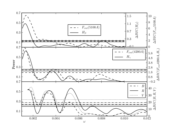
Figure 14: A comparison of GLS for spectrophotometric light curves. Horizontal lines show the 1% and 5 % significance levels for the highest peak determined by 1000 bootstrap samplings. The difference in Bayesian information criterion ($\Delta BIC$) compares single harmonic model and pure noise model. X axis depicts angular frequencies $\omega=\frac{2\pi}{period}$.

Table 1: The measured photometric magnitudes.

N	UT-date	MJD	Seeing	MR $\pm\sigma$	MV $\pm\sigma$	MB $\pm\sigma$
		2400000+	[arcsec]
1	2	3	4	5	6	7
1	28.06.03	52818.4	3.0	13.964 $\pm$ 0.027	15.230 $\pm$ 0.030	14.413 $\pm$ 0.015
2	30.06.03	52820.5	3.0	13.965 $\pm$ 0.036	15.212 $\pm$ 0.028	14.431 $\pm$ 0.014
3	31.07.03	52852.4	2.0	13.956 $\pm$ 0.028	15.232 $\pm$ 0.008	14.420 $\pm$ 0.009
4	26.08.03	52877.4	2.3	13.980 $\pm$ 0.036	15.276 $\pm$ 0.029	14.430 $\pm$ 0.026
5	01.10.03	52913.4	1.8	13.967 $\pm$ 0.036	15.283 $\pm$ 0.014	14.443 $\pm$ 0.029
6	02.10.03	52914.4	1.8	-	15.265 $\pm$ 0.035	14.462 $\pm$ 0.029
7	04.12.03	52978.2	2.0	13.978 $\pm$ 0.032	15.285 $\pm$ 0.035	14.470 $\pm$ 0.025
8	22.04.04	53117.5	2.2	13.960 $\pm$ 0.027	15.205 $\pm$ 0.014	14.405 $\pm$ 0.022
9	27.04.04	53122.5	2.0	13.951 $\pm$ 0.036	15.217 $\pm$ 0.029	14.402 $\pm$ 0.014
10	24.05.04	53143.5	2.3	13.949 $\pm$ 0.022	15.226 $\pm$ 0.033	14.579 $\pm$ 0.032
11	24.06.04	53180.5	2.3	13.914 $\pm$ 0.025	15.171 $\pm$ 0.033	14.342 $\pm$ 0.025
12	25.06.04	53181.4	1.8	13.930 $\pm$ 0.018	15.181 $\pm$ 0.025	14.334 $\pm$ 0.021
13	26.07.04	53212.4	2.0	13.894 $\pm$ 0.014	15.159 $\pm$ 0.028	14.303 $\pm$ 0.023
14	26.07.04	53213.4	2.0	13.869 $\pm$ 0.034	15.139 $\pm$ 0.019	14.297 $\pm$ 0.036
15	24.08.04	53241.4	2.0	13.862 $\pm$ 0.025	15.138 $\pm$ 0.020	14.282 $\pm$ 0.022
16	23.08.04	53242.4	2.0	13.866 $\pm$ 0.023	15.126 $\pm$ 0.029	14.272 $\pm$ 0.022
17	09.09.04	53258.4	2.8	13.838 $\pm$ 0.018	15.081 $\pm$ 0.033	14.240 $\pm$ 0.023
18	16.09.04	53265.2	2.4	13.822 $\pm$ 0.033	15.072 $\pm$ 0.025	14.219 $\pm$ 0.040
19	14.10.04	53293.4	1.9	13.761 $\pm$ 0.018	15.012 $\pm$ 0.023	14.133 $\pm$ 0.025
20	08.11.04	53318.2	1.6	13.720 $\pm$ 0.033	14.947 $\pm$ 0.022	14.099 $\pm$ 0.033
21	10.12.04	53350.1	2.0	13.722 $\pm$ 0.034	14.995 $\pm$ 0.023	14.079 $\pm$ 0.013
22	05.04.05	53466.5	1.8	13.556 $\pm$ 0.018	14.755 $\pm$ 0.034	13.918 $\pm$ 0.038
23	29.07.05	53581.5	1.5	13.519 $\pm$ 0.014	14.747 $\pm$ 0.028	13.927 $\pm$ 0.028
24	30.07.05	53582.4	2.5	13.515 $\pm$ 0.009	14.728 $\pm$ 0.028	13.890 $\pm$ 0.022
25	06.08.05	53590.3	1.2	13.524 $\pm$ 0.011	14.726 $\pm$ 0.028	13.908 $\pm$ 0.030
26	30.08.05	53613.4	2.0	13.521 $\pm$ 0.023	14.720 $\pm$ 0.030	13.894 $\pm$ 0.025
27	01.09.05	53614.4	2.0	13.513 $\pm$ 0.011	14.711 $\pm$ 0.031	13.894 $\pm$ 0.024
28	01.10.05	53645.3	1.2	13.466 $\pm$ 0.011	14.670 $\pm$ 0.033	13.854 $\pm$ 0.029
29	02.10.05	53646.3	1.4	13.465 $\pm$ 0.019	14.670 $\pm$ 0.025	13.847 $\pm$ 0.027
30	31.10.05	53675.2	3.5	13.458 $\pm$ 0.023	14.664 $\pm$ 0.038	13.807 $\pm$ 0.029
31	26.11.05	53702.2	1.8	13.423 $\pm$ 0.015	14.621 $\pm$ 0.018	13.775 $\pm$ 0.031
32	28.11.05	53703.2	2.5	13.417 $\pm$ 0.019	14.622 $\pm$ 0.022	13.785 $\pm$ 0.027
33	30.03.06	53824.5	2.5	13.435 $\pm$ 0.017	14.638 $\pm$ 0.018	13.799 $\pm$ 0.032
34	26.05.06	53882.4	1.5	13.428 $\pm$ 0.013	14.638 $\pm$ 0.028	13.807 $\pm$ 0.017
35	27.06.06	53913.5	2.5	13.454 $\pm$ 0.023	14.648 $\pm$ 0.039	13.828 $\pm$ 0.016
36	28.06.06	53914.5	2.0	13.451 $\pm$ 0.026	14.658 $\pm$ 0.035	13.805 $\pm$ 0.037
37	18.08.06	53967.3	1.8	13.452 $\pm$ 0.026	14.664 $\pm$ 0.032	13.820 $\pm$ 0.025
38	28.09.06	54007.2	2.0	13.485 $\pm$ 0.023	14.674 $\pm$ 0.031	13.859 $\pm$ 0.022
39	14.10.06	54023.2	1.7	13.495 $\pm$ 0.022	14.695 $\pm$ 0.033	13.871 $\pm$ 0.031
40	16.05.07	54236.5	1.5	-	14.699 $\pm$ 0.029	13.883 $\pm$ 0.017
41	11.06.07	54262.4	2.0	13.511 $\pm$ 0.021	14.700 $\pm$ 0.034	13.880 $\pm$ 0.010
42	10.07.07	54291.4	2.0	13.538 $\pm$ 0.028	14.696 $\pm$ 0.028	13.851 $\pm$ 0.022
43	05.09.07	54349.3	1.5	13.522 $\pm$ 0.022	14.725 $\pm$ 0.028	13.893 $\pm$ 0.023
44	06.09.07	54350.3	1.6	13.516 $\pm$ 0.024	14.717 $\pm$ 0.028	13.876 $\pm$ 0.026
45	29.03.08	54555.6	1.6	13.550 $\pm$ 0.025	14.747 $\pm$ 0.031	13.940 $\pm$ 0.011
46	27.05.08	54614.5	2.7	13.546 $\pm$ 0.026	14.785 $\pm$ 0.025	13.920 $\pm$ 0.035
47	29.10.08	54769.2	1.5	13.471 $\pm$ 0.017	14.658 $\pm$ 0.026	13.830 $\pm$ 0.025
48	30.10.08	54770.2	1.5	13.485 $\pm$ 0.028	14.672 $\pm$ 0.026	13.837 $\pm$ 0.032
49	29.11.08	54801.2	2.0	13.491 $\pm$ 0.019	14.692 $\pm$ 0.035	13.858 $\pm$ 0.026
50	30.11.08	54801.2	1.6	13.518 $\pm$ 0.019	14.710 $\pm$ 0.026	13.894 $\pm$ 0.023
51	31.05.09	54982.5	2.5	13.596 $\pm$ 0.026	14.818 $\pm$ 0.037	13.972 $\pm$ 0.020
52	30.06.09	55012.4	1.6	13.607 $\pm$ 0.021	14.818 $\pm$ 0.035	13.995 $\pm$ 0.024
53	28.07.09	55040.4	1.8	13.602 $\pm$ 0.025	14.844 $\pm$ 0.025	13.984 $\pm$ 0.038
54	28.07.09	55041.3	3.0	13.638 $\pm$ 0.032	14.857 $\pm$ 0.028	13.986 $\pm$ 0.025
55	27.08.09	55071.3	2.5	13.630 $\pm$ 0.028	14.880 $\pm$ 0.021	14.018 $\pm$ 0.016
56	24.09.09	55099.3	1.6	13.652 $\pm$ 0.018	14.894 $\pm$ 0.031	14.070 $\pm$ 0.017
57	25.09.09	55100.3	1.4	13.652 $\pm$ 0.018	14.880 $\pm$ 0.030	14.076 $\pm$ 0.023
58	26.10.09	55131.2	1.6	13.669 $\pm$ 0.027	14.903 $\pm$ 0.025	14.078 $\pm$ 0.017
59	12.11.09	55148.1	1.8	13.664 $\pm$ 0.022	14.910 $\pm$ 0.026	14.062 $\pm$ 0.015
60	13.11.09	55149.3	2.4	13.678 $\pm$ 0.015	14.893 $\pm$ 0.033	14.078 $\pm$ 0.027
61	14.04.10	55301.5	3.0	13.694 $\pm$ 0.027	14.883 $\pm$ 0.026	14.037 $\pm$ 0.024
62	08.06.10	55355.4	2.2	13.681 $\pm$ 0.024	14.899 $\pm$ 0.031	14.068 $\pm$ 0.031
63	05.07.10	55382.4	1.6	13.670 $\pm$ 0.027	14.875 $\pm$ 0.031	14.071 $\pm$ 0.020
64	02.08.10	55411.4	1.4	13.660 $\pm$ 0.022	14.896 $\pm$ 0.032	14.066 $\pm$ 0.025
65	03.08.10	55412.3	1.4	13.656 $\pm$ 0.023	14.892 $\pm$ 0.027	14.059 $\pm$ 0.026
66	26.09.10	55466.3	2.0	13.672 $\pm$ 0.026	14.888 $\pm$ 0.030	14.078 $\pm$ 0.021
67	27.09.10	55467.2	1.0	13.699 $\pm$ 0.024	14.906 $\pm$ 0.035	14.090 $\pm$ 0.024
68	31.10.10	55501.3	3.0	13.734 $\pm$ 0.032	14.980 $\pm$ 0.023	14.133 $\pm$ 0.034
69	06.12.10	55537.2	4.0	13.693 $\pm$ 0.027	14.933 $\pm$ 0.033	14.085 $\pm$ 0.027
70	29.03.11	55649.6	2.5	13.661 $\pm$ 0.018	14.873 $\pm$ 0.034	14.043 $\pm$ 0.019
71	25.06.11	55737.4	2.0	13.595 $\pm$ 0.020	14.783 $\pm$ 0.027	13.961 $\pm$ 0.017
72	23.07.11	55765.4	1.4	13.563 $\pm$ 0.023	14.754 $\pm$ 0.023	13.932 $\pm$ 0.016
73	26.08.11	55799.4	2.5	13.560 $\pm$ 0.027	14.763 $\pm$ 0.033	13.928 $\pm$ 0.024
74	27.08.11	55800.4	2.5	13.572 $\pm$ 0.020	14.766 $\pm$ 0.032	13.920 $\pm$ 0.026
75	27.09.11	55832.3	2.5	13.551 $\pm$ 0.024	14.752 $\pm$ 0.034	13.925 $\pm$ 0.017
76	28.09.11	55833.3	1.6	13.549 $\pm$ 0.014	14.755 $\pm$ 0.027	13.939 $\pm$ 0.027
77	29.12.11	55925.2	1.5	13.614 $\pm$ 0.020	14.827 $\pm$ 0.026	13.990 $\pm$ 0.020
78	23.05.12	56070.5	1.8	13.668 $\pm$ 0.017	14.889 $\pm$ 0.030	14.046 $\pm$ 0.016
79	13.06.12	56091.5	1.5	13.679 $\pm$ 0.026	14.887 $\pm$ 0.032	14.066 $\pm$ 0.022
80	14.06.12	56092.4	1.0	13.677 $\pm$ 0.026	14.884 $\pm$ 0.030	14.072 $\pm$ 0.025
81	05.05.13	56417.5	1.2	13.750 $\pm$ 0.024	14.950 $\pm$ 0.029	14.116 $\pm$ 0.027
82	06.05.13	56418.5	1.5	13.747 $\pm$ 0.029	14.968 $\pm$ 0.025	14.114 $\pm$ 0.033
83	08.07.13	56481.4	1.5	13.787 $\pm$ 0.022	14.993 $\pm$ 0.032	14.183 $\pm$ 0.024
84	09.08.13	56514.3	1.2	13.806 $\pm$ 0.014	15.043 $\pm$ 0.024	14.209 $\pm$ 0.027
85	28.08.13	56533.4	1.4	13.812 $\pm$ 0.025	15.021 $\pm$ 0.031	14.227 $\pm$ 0.031
86	29.08.13	56534.3	1.4	13.808 $\pm$ 0.021	15.043 $\pm$ 0.019	14.228 $\pm$ 0.030
87	29.10.13	56595.2	1.4	13.817 $\pm$ 0.017	15.064 $\pm$ 0.021	14.232 $\pm$ 0.028
88	30.10.13	56596.2	1.3	13.824 $\pm$ 0.012	15.069 $\pm$ 0.022	14.222 $\pm$ 0.029
89	24.12.13	56651.2	1.3	13.786 $\pm$ 0.020	15.012 $\pm$ 0.025	14.213 $\pm$ 0.022
90	29.12.13	56656.2	1.9	13.792 $\pm$ 0.019	15.016 $\pm$ 0.022	14.217 $\pm$ 0.023
91	03.01.14	56661.2	1.7	13.796 $\pm$ 0.016	15.009 $\pm$ 0.026	14.195 $\pm$ 0.014
92	09.01.14	56667.6	3.0	13.785 $\pm$ 0.033	15.047 $\pm$ 0.018	14.197 $\pm$ 0.016
93	05.04.14	56753.6	1.9	13.738 $\pm$ 0.026	14.952 $\pm$ 0.024	14.096 $\pm$ 0.022
94	23.05.14	56801.5	1.5	13.732 $\pm$ 0.026	14.945 $\pm$ 0.013	14.115 $\pm$ 0.030
95	28.07.14	56867.4	1.7	13.774 $\pm$ 0.013	14.969 $\pm$ 0.033	14.140 $\pm$ 0.026
96	22.09.14	56923.3	2.5	13.775 $\pm$ 0.020	15.000 $\pm$ 0.028	14.154 $\pm$ 0.017
97	19.10.14	56950.3	4.1	13.821 $\pm$ 0.034	15.059 $\pm$ 0.034	14.213 $\pm$ 0.027
98	20.10.14	56951.3	1.4	13.790 $\pm$ 0.018	15.007 $\pm$ 0.027	14.164 $\pm$ 0.030

Note. — Col.(1): Number. Col.(2): UT date. Col.(3): Modified Julian date (MJD). Col.(4): Mean seeing in arcsec. Cols.(5)-(7): BRV magnitudes and the corresponding errors.

Table 2: Sources of spectroscopic observations.

Observatory	Code	Tel.aperture + equipment	Aperture [arcsec]	Focus
1	2	3	4	5
SAO (Russia)	L(N)	6 m + Long slit	2.0$\times$6.0	Nasmith
SAO (Russia)	L(U)	6 m + UAGS	2.0$\times$6.0	Prime
SAO (Russia)	L(Sc)	6 m + Scorpio	1.0$\times$6.07	Prime
Guillermo Haro Observatory (México)	GHO	2.1 m + B&C	2.5$\times$6.0	Cassegrain
SAO (Russia)	Z1	1 m + GAD	4.0$\times$19.8	Cassegrain
SAO (Russia)	Z2	1 m + GAD	4.0$\times$9.45	Cassegrain
Calar Alto(Spain)	CA1	3.5 m + B&C / TWIN	2.0$\times$4.0	Cassegrain
Calar Alto(Spain)	CA2	2.2 m + B&C	2.0$\times$4.0	Cassegrain

Note. — Col.(1): Observatory. Col.(2): Code assigned to each combination of telescope + equipment used throughout this paper. Col.(3): Telescope aperture and spectrograph. Col.(4): Projected spectrograph entrance apertures (slit width$\times$slit length in arcsec). Col.(5): Focus of the telescope.

Table 3: The log of spectroscopic observations.

N	UT-date	MJD	CODE	Aperture	Sp.range	Seeing
		2400000+		[arcsec]	[${\rm\AA}$]	[arcsec]
1	2	3	4	5	6	7
1	23.07.1990	48095.0	CA1	2.0x4.0	6060-7690	1.5 - 2.5
2	07.08.1991	48476.0	CA2	2.0x4.0	5170-7650	1.5 - 2.5
3	10.08.1991	48479.0	CA2	2.0x4.0	5540-7640	1.5 - 2.5
4	09.07.1992	48813.0	CA1	2.0x4.0	5510-7690	1.5 - 2.5
5	25.08.1992	48860.0	CA2	2.0x4.0	3850-7650	1.5 - 2.5
6	01.09.1994	49597.0	CA2	2.0x4.0	5970-7690	1.5 - 2.5
7	22.02.1998	50866.6	L(N)	2.0x6.0	4690-6930	2
8	07.05.1998	50941.1	L(N)	2.0x6.0	4350-6630	3
9	26.06.1998	50990.5	Z1	4.0x19.8	5600-7240	4
10	16.07.1998	51011.3	GHO	2.5x6.0	5660-7690	2.7
11	19.09.1998	51076.4	Z1	4.0x19.8	5600-7290	2
12	22.09.1998	51079.5	GHO	2.5x6.0	5900-7690	1.8
13	10.07.1999	51370.4	L(U)	2.0x6.0	5040-7330	2
14	12.07.1999	51371.5	L(U)	2.0x6.0	5550-6680	1.5
15	03.08.1999	51393.5	Z1	4.0x19.8	5590-7300	4
16	09.08.1999	51400.4	Z1	4.0x19.8	5590-7300	2
17	03.09.1999	51425.3	L(U)	2.0x6.0	4890-7240	1.5
18	03.10.1999	51455.2	L(U)	2.0x6.0	6040-7240	1.5
19	06.10.1999	51458.2	L(U)	2.0x6.0	4900-7240	1.5
20	04.11.1999	51487.1	L(U)	2.0x6.0	5010-7670	2.5
21	09.11.1999	51492.3	GHO	2.5x6.0	4260-7480	2.5
22	25.02.2000	51560.0	GAO	2.5x6.0	4590-7690	2.5
23	26.02.2000	51600.9	GHO	2.5x6.0	4340-7570	3.0
24	24.04.2000	51658.9	GHO	2.5x6.0	4240-7460	2.7
25	25.04.2000	51659.9	GHO	2.5x6.0	4240-7460	3.0
26	24.05.2000	51688.5	GHO	2.5x6.0	4200-7370	2.5
27	25.06.2000	51720.8	GHO	2.5x6.0	4720-7690	3.0
28	22.08.2000	51779.3	Z1	4.0x19.8	5600-7290	2
29	11.09.2000	51799.3	Z1	4.0x19.8	5600-7280	2
30	16.10.2000	51833.7	GHO	2.5x6.0	4130-7280	2.3
31	30.10.2000	51848.3	Z1	4.0x19.8	5550-7230	3
32	16.11.2000	51865.2	Z1	4.0x19.8	5600-7290	2
33	01.12.2000	51880.2	Z1	4.0x19.8	5650-7290	2
34	23.01.2001	51932.6	L(U)	2.0x6.0	5740-7690	3.2
35	14.06.2001	52074.8	GHO	2.5x6.0	4100-7160	2.3
36	09.07.2001	52100.5	L(U)	2.0x6.0	5750-7690	?
37	24.08.2001	52146.4	L(U)	2.0x6.0	5750-7690	2.5
38	24.09.2001	52177.2	Z1	4.0x19.8	5600-7270	4
39	10.10.2001	52193.3	Z1	4.0x19.8	5640-7290	1
40	03.04.2002	52367.9	GHO	2.5x6.0	5760-7410	1.5
41	05.04.2002	52370.0	GHO	2.5x6.0	3850-7080	1.5
42	03.05.2002	52397.9	GHO	2.5x6.0	5700-7370	2.0
43	02.06.2002	52427.9	GHO	2.5x6.0	5760-7430	3.2
44	23.06.2002	52449.5	L(U)	2.0x6.0	5640-7690	2
45	24.06.2002	52450.4	L(U)	2.0x6.0	5640-7690	2
46	14.07.2002	52470.3	L(U)	2.0x6.0	5640-7690	1.4
47	16.07.2002	52472.3	Z1	4.0x19.8	5590-7290	1.5
48	17.08.2002	52503.8	GHO	2.5x6.0	5700-7340	2.0
49	24.09.2002	52542.2	Z1	4.0x19.8	5590-7290	2
50	13.10.2002	52561.4	L(U)	2.0x6.0	5640-7690	2.2
51	12.11.2002	52590.6	GHO	2.5x6.0	5740-7400	2.7
52	13.11.2002	52591.6	GHO	2.5x6.0	5740-7400	2.7
53	14.11.2002	52592.6	GHO	2.5x6.0	3840-7080	2.7
54	27.03.2003	52726.0	GHO	2.5x6.0	3810-7100	3.2
55	11.04.2003	52740.9	GHO	2.5x6.0	5620-7450	3.6
56	12.05.2003	52772.3	L(U)	2.0x6.0	5740-7690	1.2
57	22.05.2003	52781.9	GHO	2.5x6.0	3710-7160	3.6
58	24.05.2003	52783.9	GHO	2.5x6.0	5610-7440	3.1
59	22.06.2003	52812.9	GHO	2.5x6.0	5650-7300	2.7
60	04.09.2003	52886.7	GHO	2.5x6.0	5720-7430	2.3
61	18.10.2003	52930.6	GHO	2.5x6.0	5710-7380	1.8
62	20.10.2003	52932.6	GHO	2.5x6.0	3880-7090	1.8
63	29.02.2004	53065.4	L(U)	2.0x6.0	5800-7690	2.
64	17.03.2004	53082.0	GHO	2.5x6.0	5710-7410	2.3
65	18.03.2004	53083.0	GHO	2.5x6.0	3830-7100	2.3
66	20.05.2004	53145.9	GHO	2.5x6.0	5710-7410	2.7
67	12.06.2004	53168.9	GHO	2.5x6.0	5710-7330	1.8
68	14.06.2004	53170.5	Z2K	4.0x9.45	3750-7590	4
69	14.06.2004	53170.9	GHO	2.5x6.0	3850-7100	2.3
70	25.06.2004	53171.9	GHO	2.5x6.0	3890-7100	3.6
71	10.07.2004	53196.5	Z2K	4.0x9.45	3740-7400	4
72	11.07.2004	53197.4	Z2K	4.0x9.45	3740-7400	4
73	19.08.2004	53236.7	GHO	2.5x6.0	5710-7340	3.1
74	20.08.2004	53237.7	GHO	2.5x6.0	3810-7090	2.7
75	19.12.2004	53359.1	L(Sc)	1.0x6.07	3910-7530	2
76	20.12.2004	53360.2	Z2K	4.0x9.45	3740-7370	2
77	11.05.2005	53501.9	GHO	2.5x6.0	3810-7090	3.6
78	13.05.2005	53503.9	GHO	2.5x6.0	5710-7300	2.3
79	10.06.2005	53531.9	GHO	2.5x6.0	5710-7390	3.6
80	08.07.2005	53559.7	Z2K	4.0x9.45	3740-7330	2.7
81	10.08.2005	53593.4	Z2K	4.0x9.45	3750-7290	4
82	29.09.2005	53642.6	GHO	2.5x6.0	5750-7400	3.1
83	10.08.2005	53683.1	Z2K	4.0x9.45	3750-7370	4
84	20.04.2006	53845.9	GHO	2.5x6.0	5710-7350	2.6
85	29.06.2006	53916.3	Z2K	4.0x9.45	3750-7370	2.5
86	29.06.2006	53916.4	Z2K	4.0x9.45	3750-7370	2.5
87	31.07.2006	53948.3	Z2K	4.0x9.45	3750-7370	2
88	28.08.2006	53976.3	Z2K	4.0x9.45	3740-7390	3
89	27.10.2006	54036.3	Z2K	4.0x9.45	3740-7390	2.5
90	23.05.2007	54244.4	Z2K	4.0x9.45	3740-7390	2
91	22.06.2007	54274.4	Z2K	4.0x9.45	3740-7390	4
92	18.07.2007	54300.4	Z2K	4.0x9.45	3740-7390	3
93	20.07.2007	54302.4	Z2K	4.0x9.45	3740-7390	2.5
94	21.07.2007	54303.4	Z2K	4.0x9.45	3740-7390	2.5
95	16.08.2007	54329.4	Z2K	4.0x9.45	3740-7390	3
96	19.08.2007	54332.4	Z2K	4.0x9.45	3740-7390	2
97	19.10.2007	54393.3	Z2K	4.0x9.45	3740-7390	3
98	06.06.2008	54623.5	Z2K	4.0x9.45	3740-7390	2.5
99	22.07.2008	54670.5	L(Sc)	1.0x6.07	5640-7350	1.1
100	23.10.2008	54763.2	Z2K	4.0x9.45	3740-7390	2.5
101	15.05.2009	54967.5	Z2K	4.0x9.45	3740-7390	2.5
102	11.08.2009	55055.5	Z2K	4.0x9.45	3740-7390	4
103	13.08.2009	55057.7	Z2K	4.0x9.45	3740-7390	2.5
104	11.09.2009	55086.3	Z2K	4.0x9.45	3740-7390	2
105	10.10.2009	55115.3	Z2K	4.0x9.45	3750-7390	2.5
106	14.10.2009	55119.2	Z2K	4.0x9.45	3750-7390	2.5
107	24.11.2009	55160.2	L(Sc)	1.0x6.07	3710-7570	2.1
108	10.12.2009	55176.2	Z2K	4.0x9.45	3750-7390	3.5
109	23.12.2009	55189.2	L(Sc)	1.0x6.07	3740-7680	2.4
110	21.04.2010	55308.5	Z2K	4.0x9.45	3740-7350	5.5
111	17.06.2010	55365.5	Z2K	4.0x9.45	3740-7380	3
112	15.07.2010	55393.4	Z2K	4.0x9.45	3740-7380	2.5
113	14.11.2010	55515.1	Z2K	4.0x9.45	3740-7380	1.5
114	04.07.2011	55747.4	Z2K	4.0x9.45	3740-7380	5
115	06.08.2011	55780.5	Z2K	4.0x9.45	3750-7390	3.2
116	31.10.2011	55866.2	Z2K	4.0x9.45	3750-7390	3
117	03.11.2011	55869.1	Z2K	4.0x9.45	3750-7390	3
118	31.12.2011	55927.2	Z2K	4.0x9.45	3750-7390	4
119	22.06.2012	56101.5	Z2K	4.0x9.45	3700-7660	3.7
120	11.05.2013	56423.9	GHO	2.5x6.0	3790-7110	1.5
121	14.05.2013	56426.9	GHO	2.5x6.0	5670-7360	2.5
122	31.05.2013	56444.5	L(Sc)	1.0x6.07	3740-7680	1.5
123	07.06.2013	56450.9	GHO	2.5x6.0	3810-7110	1.8
124	11.07.2013	56485.4	Z2K	4.0x9.45	3700-7690	2.5
125	09.08.2013	56513.7	GHO	2.5x6.0	3810-7030	2.7
126	05.10.2013	56570.6	GHO	2.5x6.0	3810-7160	1.5
127	24.02.2014	56712.6	L(Sc)	1.0x6.07	3700-7260	1.7

Note. — Col.(1): Number. Col.(2): UT date. Col.(3): Modified Julian date (JD). Col.(4): CODE. Col.(5): Projected spectrograph entrance apertures. Col.(6): Wavelength range covered. Col.(7): Mean seeing in arcsec.

Table 4: Flux scale factors for optical spectra.

Sample	Aperture	Scale factor	Extended source correction
	(arcsec)	($\varphi$)	G(g)
L(U,N)	2.0$\times$6.0	1.000	0.000
L(Sc)	1.0$\times$6.07	0.976	-0.414
GHO	2.5$\times$6.0	0.951	0.000
Z1	4.0$\times$19.8	0.958$\pm$0.017	0.280$\pm$0.166
Z2	4.0$\times$9.45	1.048	0.033
CA1	2.0$\times$4.0	1.000	0.000
CA2	2.0$\times$4.0	1.000	0.000

Table 5: The measured line and continuum fluxes.

N	UT-date	JD+	F${\rm 5100}\pm\sigma$	F(H$\beta$)$\pm\sigma$	F${\rm 4200}\pm\sigma$	F(H$\gamma$)$\pm\sigma$
		2400000+	$10^{-15}\rm erg\,cm^{-2}s^{-1}$Å-1	$10^{-13}\rm erg\,cm^{-2}s^{-1}$	$10^{-15}\rm erg\,cm^{-2}s^{-1}$	$10^{-13}\rm erg\,cm^{-2}s^{-1}$
1	2	3	4	5	6	7
1	23.07.1990	48095.0	5.23 $\pm$ 0.12	11.58 $\pm$ 0.34	7.58 $\pm$ 0.24	2.60 $\pm$ 0.14
2	07.08.1991	48476.0	5.59 $\pm$ 0.13	11.29 $\pm$ 0.33	7.34 $\pm$ 0.24	2.34 $\pm$ 0.12
3	10.08.1991	48479.0	5.42 $\pm$ 0.13	10.81 $\pm$ 0.32	7.20 $\pm$ 0.23	2.28 $\pm$ 0.12
4	09.07.1992	48813.0	5.19 $\pm$ 0.12	11.65 $\pm$ 0.34	6.50 $\pm$ 0.21	2.39 $\pm$ 0.12
5	25.08.1992	48860.0	5.50 $\pm$ 0.13	12.32 $\pm$ 0.36	12.36 $\pm$ 0.40	2.84 $\pm$ 0.15
6	01.09.1994	49597.0	6.31 $\pm$ 0.15	11.59 $\pm$ 0.34	-	-
7	22.02.1998	50866.6	8.43 $\pm$ 0.20	12.55 $\pm$ 0.37	-	-
8	07.05.1998	50941.1	8.76 $\pm$ 0.21	12.23 $\pm$ 0.36	10.65 $\pm$ 0.34	2.61 $\pm$ 0.14
9	26.06.1998	50990.5	8.25 $\pm$ 0.19	12.66 $\pm$ 0.37	-	-
10	16.07.1998	51011.3	8.15 $\pm$ 0.19	12.78 $\pm$ 0.37	-	-
11	19.09.1998	51076.4	7.52 $\pm$ 0.18	12.13 $\pm$ 0.36	-	-
12	22.09.1998	51079.5	7.64 $\pm$ 0.18	12.30 $\pm$ 0.36	-	-
13	10.07.1999	51370.4	7.58 $\pm$ 0.18	13.18 $\pm$ 0.39	9.78 $\pm$ 0.31	2.40 $\pm$ 0.12
14	12.07.1999	51371.5	8.03 $\pm$ 0.19	13.81 $\pm$ 0.40	-	-
15	03.08.1999	51393.5	6.90 $\pm$ 0.16	12.93 $\pm$ 0.38	-	-
16	09.08.1999	51400.4	7.25 $\pm$ 0.17	13.46 $\pm$ 0.39	-	-
17	03.09.1999	51425.3	7.06 $\pm$ 0.17	12.20 $\pm$ 0.36	9.95 $\pm$ 0.32	2.56 $\pm$ 0.13
18	03.10.1999	51455.2	7.61 $\pm$ 0.18	12.41 $\pm$ 0.36	-	-
19	06.10.1999	51458.2	7.70 $\pm$ 0.18	12.98 $\pm$ 0.38	11.80 $\pm$ 0.38	3.27 $\pm$ 0.17
20	04.11.1999	51487.1	7.63 $\pm$ 0.18	12.37 $\pm$ 0.36	10.65 $\pm$ 0.34	2.77 $\pm$ 0.14
21	09.11.1999	51492.3	7.12 $\pm$ 0.17	12.37 $\pm$ 0.36	10.89 $\pm$ 0.35	2.45 $\pm$ 0.13
22	25.02.2000	51599.0	6.39 $\pm$ 0.15	11.57 $\pm$ 0.34	8.42 $\pm$ 0.27	2.42 $\pm$ 0.13
23	26.02.2000	51600.9	6.38 $\pm$ 0.15	11.58 $\pm$ 0.34	8.76 $\pm$ 0.28	2.34 $\pm$ 0.12
24	24.04.2000	51658.9	6.69 $\pm$ 0.16	11.97 $\pm$ 0.35	8.71 $\pm$ 0.28	2.39 $\pm$ 0.12
25	25.04.2000	51659.9	6.68 $\pm$ 0.16	11.95 $\pm$ 0.35	8.82 $\pm$ 0.28	2.44 $\pm$ 0.13
26	24.05.2000	51688.5	6.46 $\pm$ 0.15	12.00 $\pm$ 0.35	9.00 $\pm$ 0.29	2.46 $\pm$ 0.13
27	25.06.2000	51720.8	6.70 $\pm$ 0.16	11.73 $\pm$ 0.34	8.97 $\pm$ 0.29	2.40 $\pm$ 0.12
28	22.08.2000	51779.3	6.12 $\pm$ 0.14	10.96 $\pm$ 0.32	-	-
29	11.09.2000	51799.3	6.17 $\pm$ 0.14	11.27 $\pm$ 0.33	-	-
30	16.10.2000	51833.7	6.25 $\pm$ 0.15	11.79 $\pm$ 0.35	8.15 $\pm$ 0.26	2.61 $\pm$ 0.14
31	30.10.2000	51848.3	6.25 $\pm$ 0.15	11.98 $\pm$ 0.35	-	-
32	16.11.2000	51865.2	6.50 $\pm$ 0.15	11.87 $\pm$ 0.35	-	-
33	01.12.2000	51880.2	6.20 $\pm$ 0.15	12.35 $\pm$ 0.36	-	-
34	23.01.2001	51932.6	6.44 $\pm$ 0.15	11.93 $\pm$ 0.35	-	-
35	14.06.2001	52074.8	5.99 $\pm$ 0.14	11.21 $\pm$ 0.33	8.37 $\pm$ 0.27	2.25 $\pm$ 0.12
36	09.07.2001	52100.5	7.13 $\pm$ 0.17	12.54 $\pm$ 0.37	-	-
37	24.08.2001	52146.4	6.71 $\pm$ 0.16	12.32 $\pm$ 0.36	-	-
38	24.09.2001	52177.2	6.40 $\pm$ 0.15	12.66 $\pm$ 0.37	-	-
39	10.10.2001	52193.3	5.98 $\pm$ 0.14	11.40 $\pm$ 0.33	-	-
40	03.04.2002	52367.9	5.90 $\pm$ 0.14	11.75 $\pm$ 0.34	-	-
41	05.04.2002	52369.0	5.87 $\pm$ 0.14	11.28 $\pm$ 0.33	8.07 $\pm$ 0.26	2.28 $\pm$ 0.12
42	03.05.2002	52397.9	5.95 $\pm$ 0.14	11.36 $\pm$ 0.33	-	-
43	02.06.2002	52427.9	5.68 $\pm$ 0.13	11.30 $\pm$ 0.33	-	-
44	23.06.2002	52449.5	6.55 $\pm$ 0.15	11.54 $\pm$ 0.34	-	-
45	24.06.2002	52450.4	7.22 $\pm$ 0.17	12.83 $\pm$ 0.38	-	-
46	14.07.2002	52470.3	6.14 $\pm$ 0.14	11.98 $\pm$ 0.35	-	-
47	16.07.2002	52472.3	6.25 $\pm$ 0.15	12.14 $\pm$ 0.36	-	-
48	17.08.2002	52503.8	5.85 $\pm$ 0.14	11.20 $\pm$ 0.33	-	-
49	24.09.2002	52542.2	7.54 $\pm$ 0.18	13.30 $\pm$ 0.39	-	-
50	13.10.2002	52561.4	6.20 $\pm$ 0.15	11.73 $\pm$ 0.34	-	-
51	12.11.2002	52590.6	5.61 $\pm$ 0.13	11.73 $\pm$ 0.34	-	-
52	13.11.2002	52591.6	5.70 $\pm$ 0.13	11.68 $\pm$ 0.34	-	-
53	14.11.2002	52592.6	5.65 $\pm$ 0.13	11.67 $\pm$ 0.34	7.82 $\pm$ 0.25	2.38 $\pm$ 0.12
54	27.03.2003	52725.0	6.12 $\pm$ 0.14	11.47 $\pm$ 0.34	6.96 $\pm$ 0.22	2.44 $\pm$ 0.13
55	11.04.2003	52740.9	5.86 $\pm$ 0.14	12.27 $\pm$ 0.36	-	-
56	12.05.2003	52772.3	6.00 $\pm$ 0.14	12.03 $\pm$ 0.35	-	-
57	22.05.2003	52781.9	5.57 $\pm$ 0.13	11.90 $\pm$ 0.35	7.75 $\pm$ 0.25	2.46 $\pm$ 0.13
58	24.05.2003	52783.9	5.31 $\pm$ 0.12	11.38 $\pm$ 0.33	-	-
59	22.06.2003	52812.9	5.46 $\pm$ 0.13	12.52 $\pm$ 0.37	-	-
60	04.09.2003	52886.7	5.00 $\pm$ 0.12	12.14 $\pm$ 0.36	-	-
61	18.10.2003	52930.6	4.94 $\pm$ 0.12	12.55 $\pm$ 0.37	-	-
62	20.10.2003	52932.6	5.06 $\pm$ 0.12	11.91 $\pm$ 0.35	7.69 $\pm$ 0.25	2.34 $\pm$ 0.12
63	29.02.2004	53065.4	5.63 $\pm$ 0.13	12.01 $\pm$ 0.35	-	-
64	17.03.2004	53082.0	5.16 $\pm$ 0.12	12.01 $\pm$ 0.35	-	-
65	18.03.2004	53083.0	4.90 $\pm$ 0.11	10.82 $\pm$ 0.32	6.51 $\pm$ 0.21	1.96 $\pm$ 0.10
66	20.05.2004	53145.9	5.24 $\pm$ 0.12	11.31 $\pm$ 0.33	-	-
67	12.06.2004	53168.9	5.55 $\pm$ 0.13	11.54 $\pm$ 0.34	-	-
68	14.06.2004	53170.5	5.71 $\pm$ 0.13	11.56 $\pm$ 0.34	-	-
69	14.06.2004	53170.9	5.78 $\pm$ 0.14	11.61 $\pm$ 0.34	8.09 $\pm$ 0.26	2.12 $\pm$ 0.11
70	25.06.2004	53171.9	5.85 $\pm$ 0.14	11.64 $\pm$ 0.34	8.34 $\pm$ 0.27	2.08 $\pm$ 0.11
71	10.07.2004	53196.5	7.39 $\pm$ 0.17	14.08 $\pm$ 0.41	9.89 $\pm$ 0.32	2.50 $\pm$ 0.13
72	11.07.2004	53197.4	6.87 $\pm$ 0.16	13.18 $\pm$ 0.39	9.21 $\pm$ 0.30	2.23 $\pm$ 0.12
73	19.08.2004	53236.7	6.19 $\pm$ 0.14	11.79 $\pm$ 0.35	-	-
74	20.08.2004	53237.7	5.74 $\pm$ 0.13	11.11 $\pm$ 0.33	8.40 $\pm$ 0.27	2.10 $\pm$ 0.11
75	19.12.2004	53359.1	7.40 $\pm$ 0.17	11.69 $\pm$ 0.34	10.33 $\pm$ 0.33	2.11 $\pm$ 0.11
76	20.12.2004	53360.2	7.40 $\pm$ 0.17	12.25 $\pm$ 0.36	-	-
77	11.05.2005	53501.9	8.02 $\pm$ 0.19	11.74 $\pm$ 0.34	11.02 $\pm$ 0.35	2.42 $\pm$ 0.13
78	13.05.2005	53503.9	8.07 $\pm$ 0.19	12.11 $\pm$ 0.35	-	-
79	10.06.2005	53531.9	7.88 $\pm$ 0.18	12.43 $\pm$ 0.36	-	-
80	08.07.2005	53559.7	8.83 $\pm$ 0.21	12.61 $\pm$ 0.37	12.25 $\pm$ 0.39	3.02 $\pm$ 0.16
81	10.08.2005	53593.4	8.54 $\pm$ 0.20	12.68 $\pm$ 0.37	12.04 $\pm$ 0.39	2.91 $\pm$ 0.15
82	29.09.2005	53642.6	8.33 $\pm$ 0.20	13.05 $\pm$ 0.38	-	-
83	10.08.2005	53683.1	10.64 $\pm$ 0.25	13.66 $\pm$ 0.40	13.44 $\pm$ 0.43	3.41 $\pm$ 0.18
84	20.04.2006	53845.9	8.65 $\pm$ 0.20	13.22 $\pm$ 0.39	-	-
85	29.06.2006	53916.3	9.71 $\pm$ 0.23	13.37 $\pm$ 0.39	13.83 $\pm$ 0.45	3.78 $\pm$ 0.20
86	29.06.2006	53916.4	9.94 $\pm$ 0.23	13.78 $\pm$ 0.40	12.75 $\pm$ 0.41	3.35 $\pm$ 0.17
87	31.07.2006	53948.3	10.03 $\pm$ 0.23	14.06 $\pm$ 0.41	13.90 $\pm$ 0.45	3.54 $\pm$ 0.18
88	28.08.2006	53976.3	9.23 $\pm$ 0.22	13.44 $\pm$ 0.39	13.77 $\pm$ 0.44	3.56 $\pm$ 0.18
89	27.10.2006	54036.3	10.30 $\pm$ 0.24	13.63 $\pm$ 0.40	13.50 $\pm$ 0.43	4.16 $\pm$ 0.22
90	23.05.2007	54244.4	8.41 $\pm$ 0.20	13.07 $\pm$ 0.38	11.98 $\pm$ 0.39	3.46 $\pm$ 0.18
91	22.06.2007	54274.4	8.84 $\pm$ 0.21	13.37 $\pm$ 0.39	11.63 $\pm$ 0.37	3.24 $\pm$ 0.17
92	18.07.2007	54300.4	8.43 $\pm$ 0.20	12.30 $\pm$ 0.36	11.39 $\pm$ 0.37	3.88 $\pm$ 0.20
93	20.07.2007	54302.4	9.09 $\pm$ 0.21	13.68 $\pm$ 0.40	12.09 $\pm$ 0.39	3.34 $\pm$ 0.17
94	21.07.2007	54303.4	9.09 $\pm$ 0.21	13.54 $\pm$ 0.40	12.65 $\pm$ 0.41	3.43 $\pm$ 0.18
95	16.08.2007	54329.4	9.85 $\pm$ 0.23	14.69 $\pm$ 0.43	12.62 $\pm$ 0.41	3.33 $\pm$ 0.17
96	19.08.2007	54332.4	9.39 $\pm$ 0.22	13.97 $\pm$ 0.41	12.83 $\pm$ 0.41	3.48 $\pm$ 0.18
97	19.10.2007	54393.3	8.39 $\pm$ 0.20	13.28 $\pm$ 0.39	13.49 $\pm$ 0.43	4.20 $\pm$ 0.22
98	06.06.2008	54623.5	8.61 $\pm$ 0.20	13.51 $\pm$ 0.40	11.74 $\pm$ 0.38	3.21 $\pm$ 0.17
99	22.07.2008	54670.5	7.78 $\pm$ 0.18	11.27 $\pm$ 0.33	-	-
100	23.10.2008	54763.2	9.11 $\pm$ 0.21	12.53 $\pm$ 0.37	13.22 $\pm$ 0.43	3.32 $\pm$ 0.17
101	15.05.2009	54967.5	9.01 $\pm$ 0.21	14.44 $\pm$ 0.42	12.05 $\pm$ 0.39	3.65 $\pm$ 0.19
102	11.08.2009	55055.5	8.48 $\pm$ 0.20	14.03 $\pm$ 0.41	11.62 $\pm$ 0.37	3.70 $\pm$ 0.19
103	13.08.2009	55057.7	8.41 $\pm$ 0.20	14.07 $\pm$ 0.41	11.91 $\pm$ 0.38	3.80 $\pm$ 0.20
104	11.09.2009	55086.3	7.86 $\pm$ 0.18	13.63 $\pm$ 0.40	10.52 $\pm$ 0.34	3.53 $\pm$ 0.18
105	10.10.2009	55115.3	8.48 $\pm$ 0.20	15.20 $\pm$ 0.45	11.98 $\pm$ 0.39	3.61 $\pm$ 0.19
106	14.10.2009	55119.2	7.81 $\pm$ 0.18	14.19 $\pm$ 0.42	10.87 $\pm$ 0.35	3.32 $\pm$ 0.17
107	24.11.2009	55160.2	7.47 $\pm$ 0.17	13.25 $\pm$ 0.39	11.07 $\pm$ 0.36	3.25 $\pm$ 0.17
108	10.12.2009	55176.2	8.12 $\pm$ 0.19	14.67 $\pm$ 0.43	10.76 $\pm$ 0.35	3.28 $\pm$ 0.17
109	23.12.2009	55189.2	7.75 $\pm$ 0.18	13.22 $\pm$ 0.39	9.26 $\pm$ 0.30	2.80 $\pm$ 0.15
110	21.04.2010	55308.5	7.96 $\pm$ 0.19	14.40 $\pm$ 0.42	12.25 $\pm$ 0.39	4.01 $\pm$ 0.21
111	17.06.2010	55365.5	7.56 $\pm$ 0.18	12.70 $\pm$ 0.37	10.62 $\pm$ 0.34	3.00 $\pm$ 0.16
112	15.07.2010	55393.4	7.40 $\pm$ 0.17	13.19 $\pm$ 0.39	9.98 $\pm$ 0.32	2.82 $\pm$ 0.15
113	14.11.2010	55515.1	8.09 $\pm$ 0.19	13.84 $\pm$ 0.41	10.89 $\pm$ 0.35	2.94 $\pm$ 0.15
114	04.07.2011	55747.4	8.76 $\pm$ 0.20	12.33 $\pm$ 0.36	11.87 $\pm$ 0.38	3.46 $\pm$ 0.18
115	06.08.2011	55780.5	8.98 $\pm$ 0.21	13.29 $\pm$ 0.39	13.00 $\pm$ 0.42	3.22 $\pm$ 0.17
116	31.10.2011	55866.2	8.71 $\pm$ 0.20	12.74 $\pm$ 0.37	12.28 $\pm$ 0.40	3.10 $\pm$ 0.16
117	03.11.2011	55869.1	8.57 $\pm$ 0.20	13.19 $\pm$ 0.39	12.11 $\pm$ 0.39	3.02 $\pm$ 0.16
118	31.12.2011	55927.2	8.71 $\pm$ 0.20	12.42 $\pm$ 0.36	11.24 $\pm$ 0.36	3.29 $\pm$ 0.17
119	22.06.2012	56101.5	7.47 $\pm$ 0.17	13.16 $\pm$ 0.39	11.02 $\pm$ 0.35	2.90 $\pm$ 0.15
120	11.05.2013	56423.9	6.26 $\pm$ 0.15	11.17 $\pm$ 0.33	8.33 $\pm$ 0.27	2.49 $\pm$ 0.13
121	14.05.2013	56426.9	6.41 $\pm$ 0.15	11.68 $\pm$ 0.34	-	-
122	31.05.2013	56444.5	7.32 $\pm$ 0.17	12.80 $\pm$ 0.38	9.36 $\pm$ 0.30	2.86 $\pm$ 0.15
123	07.06.2013	56450.9	6.06 $\pm$ 0.14	11.37 $\pm$ 0.33	8.69 $\pm$ 0.28	2.48 $\pm$ 0.13
124	11.07.2013	56485.4	6.83 $\pm$ 0.16	12.89 $\pm$ 0.38	9.94 $\pm$ 0.32	2.56 $\pm$ 0.13
125	09.08.2013	56513.7	5.76 $\pm$ 0.13	11.57 $\pm$ 0.34	8.78 $\pm$ 0.28	2.31 $\pm$ 0.12
126	05.10.2013	56570.6	5.74 $\pm$ 0.13	11.20 $\pm$ 0.33	7.94 $\pm$ 0.26	2.37 $\pm$ 0.12
127	24.02.2014	56712.6	7.47 $\pm$ 0.17	12.22 $\pm$ 0.36	9.99 $\pm$ 0.32	2.31 $\pm$ 0.12

Table 6: Estimates of the mean errors for H$\beta$ and H$\gamma$ total-line fluxes and for H$\beta$ broad-line segment fluxes.

Line	Spectral Region	Spectral Region	$\sigma\pm$e	$V_{r}$ region	$|V_{\rm red}-V_{\rm blue}|$
	[Å] (obs)	[Å] (rest)	[%]	km s-1	km s-1
cont 5100	6601-6631	5089-5111	2.3 $\pm$2.0	-	-
cont 4200	5459-5489	4208-4231	3.2 $\pm$2.1	-	-
H$\beta$ - total	6170-6620	4756-5103	2.9 $\pm$2.1	(-6423) - (+14988)	21411
H$\gamma$ - total	5550-5770	4278-4448	5.2 $\pm$3.1	(-4763) - (+7460)	12223
H$\beta$ - broad	6170-6620	4756-5103	2.9 $\pm$2.1	(-6423) - (+14988)	21411
H$\beta$ - blue	6199-6284	4779-4844	4.9$\pm$3.8	(-6089) - (-2091)	3998
H$\beta$ - core	6285-6369	4845-4910	3.1$\pm$3.0	(-2030) - (+1968)	3998
H$\beta$ - red	6371-6456	4911-4977	4.1$\pm$3.2	(+2030) - (+6088)	4058
H$\beta$ - far red	6457-6551	4978-5050	6.0$\pm$4.6	(+6150) - (+10578)	4428

Note. — Col.(1): Measured continuum/line/line-segment. Col.(2): Observed wavelength range. Col.(3): Rest-frame wavelength range. Col.(4): Estimated error and its standard deviation. Col.(5): Velocity range . Col.(6): Velocity range width.

Table 7: The measured broad-line and line-segment fluxes of H$\beta$ in units of $10^{-13}\rm erg\,cm^{-2}s^{-1}$.

N	UT-date	JD+	F(H$\beta$)broad	F(H$\beta$)core	F(H$\beta$)red	F(H$\beta$)far red
		2400000+
1	2	3	4	5	6	7
1	48095.00	7.171 $\pm$0.205	0.861 $\pm$ 0.042	3.672 $\pm$ 0.114	1.838 $\pm$ 0.075	0.704 $\pm$ 0.042
2	48476.00	6.979 $\pm$0.200	0.822 $\pm$ 0.040	3.714 $\pm$ 0.115	1.731 $\pm$ 0.071	0.638 $\pm$ 0.038
3	48479.00	6.427 $\pm$0.184	0.673 $\pm$ 0.033	3.466 $\pm$ 0.107	1.563 $\pm$ 0.064	0.603 $\pm$ 0.036
4	48813.00	7.235 $\pm$0.207	0.763 $\pm$ 0.037	3.806 $\pm$ 0.118	1.910 $\pm$ 0.078	0.717 $\pm$ 0.043
5	48860.00	7.702 $\pm$0.220	0.805 $\pm$ 0.040	4.024 $\pm$ 0.125	1.960 $\pm$ 0.080	0.802 $\pm$ 0.048
6	49597.00	7.060 $\pm$0.202	0.763 $\pm$ 0.037	3.541 $\pm$ 0.110	1.917 $\pm$ 0.079	0.724 $\pm$ 0.043
7	50866.58	8.024 $\pm$0.229	0.842 $\pm$ 0.041	4.128 $\pm$ 0.128	2.131 $\pm$ 0.087	0.821 $\pm$ 0.049
8	50941.07	7.740 $\pm$0.221	0.783 $\pm$ 0.038	4.000 $\pm$ 0.124	2.076 $\pm$ 0.085	0.791 $\pm$ 0.047
9	50990.51	8.058 $\pm$0.230	1.084 $\pm$ 0.053	4.130 $\pm$ 0.128	1.905 $\pm$ 0.078	0.850 $\pm$ 0.051
10	51011.33	8.636 $\pm$0.247	1.046 $\pm$ 0.051	4.299 $\pm$ 0.133	2.424 $\pm$ 0.099	0.751 $\pm$ 0.045
11	51076.36	7.734 $\pm$0.221	1.008 $\pm$ 0.049	3.992 $\pm$ 0.124	1.978 $\pm$ 0.081	0.757 $\pm$ 0.045
12	51079.48	8.027 $\pm$0.230	0.937 $\pm$ 0.046	4.030 $\pm$ 0.125	2.176 $\pm$ 0.089	0.775 $\pm$ 0.046
13	51370.44	8.599 $\pm$0.246	0.938 $\pm$ 0.046	4.368 $\pm$ 0.135	2.358 $\pm$ 0.097	0.850 $\pm$ 0.051
14	51371.55	9.347 $\pm$0.267	0.978 $\pm$ 0.048	4.718 $\pm$ 0.146	2.533 $\pm$ 0.104	1.008 $\pm$ 0.060
15	51393.51	8.402 $\pm$0.240	1.110 $\pm$ 0.054	4.282 $\pm$ 0.133	2.076 $\pm$ 0.085	0.876 $\pm$ 0.053
16	51400.44	8.815 $\pm$0.252	1.177 $\pm$ 0.058	4.444 $\pm$ 0.138	2.211 $\pm$ 0.091	0.867 $\pm$ 0.052
17	51425.32	8.034 $\pm$0.230	1.001 $\pm$ 0.049	3.957 $\pm$ 0.123	2.272 $\pm$ 0.093	0.716 $\pm$ 0.043
18	51455.19	7.975 $\pm$0.228	0.726 $\pm$ 0.036	4.189 $\pm$ 0.130	2.076 $\pm$ 0.085	0.826 $\pm$ 0.050
19	51458.22	8.616 $\pm$0.246	1.082 $\pm$ 0.053	4.365 $\pm$ 0.135	2.302 $\pm$ 0.094	0.794 $\pm$ 0.048
20	51487.14	7.854 $\pm$0.225	0.877 $\pm$ 0.043	4.172 $\pm$ 0.129	2.060 $\pm$ 0.084	0.681 $\pm$ 0.041
21	51492.29	7.981 $\pm$0.228	0.886 $\pm$ 0.043	4.075 $\pm$ 0.126	2.122 $\pm$ 0.087	0.774 $\pm$ 0.046
22	51599.96	7.378 $\pm$0.211	0.794 $\pm$ 0.039	3.790 $\pm$ 0.117	1.946 $\pm$ 0.080	0.740 $\pm$ 0.044
23	51600.93	7.374 $\pm$0.211	0.779 $\pm$ 0.038	3.781 $\pm$ 0.117	1.930 $\pm$ 0.079	0.758 $\pm$ 0.045
24	51658.94	7.750 $\pm$0.222	0.809 $\pm$ 0.040	3.961 $\pm$ 0.123	2.060 $\pm$ 0.084	0.790 $\pm$ 0.047
25	51659.90	7.741 $\pm$0.221	0.832 $\pm$ 0.041	3.954 $\pm$ 0.122	2.065 $\pm$ 0.085	0.765 $\pm$ 0.046
26	51688.54	7.758 $\pm$0.222	0.855 $\pm$ 0.042	3.973 $\pm$ 0.123	2.085 $\pm$ 0.085	0.726 $\pm$ 0.044
27	51720.75	7.576 $\pm$0.217	0.863 $\pm$ 0.042	3.859 $\pm$ 0.119	2.131 $\pm$ 0.087	0.630 $\pm$ 0.038
28	51779.30	6.743 $\pm$0.193	0.828 $\pm$ 0.041	3.569 $\pm$ 0.111	1.783 $\pm$ 0.073	0.546 $\pm$ 0.033
29	51799.30	7.077 $\pm$0.202	0.826 $\pm$ 0.041	3.655 $\pm$ 0.113	1.845 $\pm$ 0.076	0.644 $\pm$ 0.039
30	51833.65	7.597 $\pm$0.217	0.799 $\pm$ 0.039	3.927 $\pm$ 0.122	2.079 $\pm$ 0.085	0.701 $\pm$ 0.042
31	51848.33	7.597 $\pm$0.217	0.946 $\pm$ 0.046	3.903 $\pm$ 0.121	2.010 $\pm$ 0.082	0.711 $\pm$ 0.043
32	51865.19	7.508 $\pm$0.215	0.937 $\pm$ 0.046	3.821 $\pm$ 0.118	1.930 $\pm$ 0.079	0.745 $\pm$ 0.045
33	51880.18	7.982 $\pm$0.228	1.066 $\pm$ 0.052	4.021 $\pm$ 0.124	2.065 $\pm$ 0.085	0.750 $\pm$ 0.045
34	51932.65	7.450 $\pm$0.213	0.788 $\pm$ 0.039	3.812 $\pm$ 0.118	2.040 $\pm$ 0.084	0.718 $\pm$ 0.043
35	52074.79	6.951 $\pm$0.199	0.718 $\pm$ 0.035	3.587 $\pm$ 0.111	1.921 $\pm$ 0.079	0.622 $\pm$ 0.037
36	52100.48	8.157 $\pm$0.233	0.947 $\pm$ 0.046	4.202 $\pm$ 0.130	2.167 $\pm$ 0.089	0.764 $\pm$ 0.046
37	52146.38	7.889 $\pm$0.226	0.857 $\pm$ 0.042	4.013 $\pm$ 0.124	2.165 $\pm$ 0.089	0.766 $\pm$ 0.046
38	52177.21	8.086 $\pm$0.231	0.978 $\pm$ 0.048	4.195 $\pm$ 0.130	2.124 $\pm$ 0.087	0.767 $\pm$ 0.046
39	52193.26	7.342 $\pm$0.210	0.869 $\pm$ 0.043	3.770 $\pm$ 0.117	1.952 $\pm$ 0.080	0.726 $\pm$ 0.044
40	52367.89	7.448 $\pm$0.213	0.850 $\pm$ 0.042	3.710 $\pm$ 0.115	2.022 $\pm$ 0.083	0.750 $\pm$ 0.045
41	52369.97	7.195 $\pm$0.206	0.712 $\pm$ 0.035	3.665 $\pm$ 0.113	2.072 $\pm$ 0.085	0.675 $\pm$ 0.041
42	52397.86	7.060 $\pm$0.202	0.802 $\pm$ 0.039	3.505 $\pm$ 0.108	1.933 $\pm$ 0.079	0.726 $\pm$ 0.044
43	52427.87	7.016 $\pm$0.201	0.722 $\pm$ 0.035	3.540 $\pm$ 0.110	1.926 $\pm$ 0.079	0.708 $\pm$ 0.043
44	52449.48	7.058 $\pm$0.202	0.678 $\pm$ 0.033	3.599 $\pm$ 0.111	2.003 $\pm$ 0.082	0.694 $\pm$ 0.042
45	52450.43	8.372 $\pm$0.239	0.808 $\pm$ 0.040	4.256 $\pm$ 0.132	2.424 $\pm$ 0.099	0.783 $\pm$ 0.047
46	52470.34	7.468 $\pm$0.214	0.769 $\pm$ 0.038	3.771 $\pm$ 0.117	2.083 $\pm$ 0.085	0.742 $\pm$ 0.045
47	52472.31	7.584 $\pm$0.217	0.888 $\pm$ 0.044	3.735 $\pm$ 0.116	2.041 $\pm$ 0.084	0.780 $\pm$ 0.047
48	52503.76	7.012 $\pm$0.201	0.767 $\pm$ 0.038	3.522 $\pm$ 0.109	1.998 $\pm$ 0.082	0.647 $\pm$ 0.039
49	52542.23	8.464 $\pm$0.242	0.840 $\pm$ 0.041	4.211 $\pm$ 0.130	2.334 $\pm$ 0.096	0.888 $\pm$ 0.053
50	52561.42	7.379 $\pm$0.211	0.686 $\pm$ 0.034	3.837 $\pm$ 0.119	2.118 $\pm$ 0.087	0.666 $\pm$ 0.040
51	52590.59	7.418 $\pm$0.212	0.809 $\pm$ 0.040	3.722 $\pm$ 0.115	2.019 $\pm$ 0.083	0.737 $\pm$ 0.044
52	52591.59	7.387 $\pm$0.211	0.801 $\pm$ 0.039	3.685 $\pm$ 0.114	2.043 $\pm$ 0.084	0.742 $\pm$ 0.045
53	52592.63	7.331 $\pm$0.210	0.772 $\pm$ 0.038	3.700 $\pm$ 0.115	2.044 $\pm$ 0.084	0.700 $\pm$ 0.042
54	52725.98	7.150 $\pm$0.204	0.755 $\pm$ 0.037	3.679 $\pm$ 0.114	1.920 $\pm$ 0.079	0.676 $\pm$ 0.041
55	52740.95	7.901 $\pm$0.226	0.820 $\pm$ 0.040	3.967 $\pm$ 0.123	2.190 $\pm$ 0.090	0.804 $\pm$ 0.048
56	52772.31	7.471 $\pm$0.214	0.807 $\pm$ 0.040	3.693 $\pm$ 0.114	2.056 $\pm$ 0.084	0.783 $\pm$ 0.047
57	52781.88	7.579 $\pm$0.217	0.790 $\pm$ 0.039	3.795 $\pm$ 0.118	2.089 $\pm$ 0.086	0.760 $\pm$ 0.046
58	52783.91	7.143 $\pm$0.204	0.784 $\pm$ 0.038	3.606 $\pm$ 0.112	1.916 $\pm$ 0.078	0.728 $\pm$ 0.044
59	52812.94	8.071 $\pm$0.231	0.920 $\pm$ 0.045	3.945 $\pm$ 0.122	2.165 $\pm$ 0.089	0.860 $\pm$ 0.052
60	52886.74	7.876 $\pm$0.225	0.972 $\pm$ 0.048	3.846 $\pm$ 0.119	2.150 $\pm$ 0.088	0.790 $\pm$ 0.047
61	52930.59	8.198 $\pm$0.234	0.963 $\pm$ 0.047	3.974 $\pm$ 0.123	2.294 $\pm$ 0.094	0.817 $\pm$ 0.049
62	52932.61	7.624 $\pm$0.218	0.829 $\pm$ 0.041	3.789 $\pm$ 0.117	2.119 $\pm$ 0.087	0.777 $\pm$ 0.047
63	53065.42	7.360 $\pm$0.211	0.725 $\pm$ 0.036	3.664 $\pm$ 0.113	2.045 $\pm$ 0.084	0.777 $\pm$ 0.047
64	53082.01	7.509 $\pm$0.215	0.759 $\pm$ 0.037	3.699 $\pm$ 0.115	2.103 $\pm$ 0.086	0.777 $\pm$ 0.047
65	53083.01	6.665 $\pm$0.191	0.731 $\pm$ 0.036	3.228 $\pm$ 0.100	1.850 $\pm$ 0.076	0.713 $\pm$ 0.043
66	53145.88	7.007 $\pm$0.200	0.841 $\pm$ 0.041	3.468 $\pm$ 0.107	1.921 $\pm$ 0.079	0.661 $\pm$ 0.040
67	53168.89	7.182 $\pm$0.205	0.782 $\pm$ 0.038	3.585 $\pm$ 0.111	2.001 $\pm$ 0.082	0.686 $\pm$ 0.041
68	53170.54	7.083 $\pm$0.203	0.742 $\pm$ 0.036	3.438 $\pm$ 0.106	1.959 $\pm$ 0.080	0.759 $\pm$ 0.046
69	53170.88	7.120 $\pm$0.204	0.799 $\pm$ 0.039	3.638 $\pm$ 0.113	2.022 $\pm$ 0.083	0.653 $\pm$ 0.039
70	53171.91	7.110 $\pm$0.203	0.719 $\pm$ 0.035	3.458 $\pm$ 0.107	1.992 $\pm$ 0.082	0.788 $\pm$ 0.047
71	53196.51	8.810 $\pm$0.252	0.854 $\pm$ 0.042	4.408 $\pm$ 0.136	2.317 $\pm$ 0.095	1.093 $\pm$ 0.066
72	53197.39	8.248 $\pm$0.236	0.798 $\pm$ 0.039	4.026 $\pm$ 0.125	2.359 $\pm$ 0.097	0.878 $\pm$ 0.053
73	53236.72	7.346 $\pm$0.210	0.840 $\pm$ 0.041	3.601 $\pm$ 0.111	2.039 $\pm$ 0.084	0.721 $\pm$ 0.043
74	53237.73	6.956 $\pm$0.199	0.729 $\pm$ 0.036	3.446 $\pm$ 0.107	1.965 $\pm$ 0.080	0.671 $\pm$ 0.040
75	53359.11	7.116 $\pm$0.204	0.780 $\pm$ 0.038	3.494 $\pm$ 0.108	2.013 $\pm$ 0.082	0.691 $\pm$ 0.041
76	53360.19	7.509 $\pm$0.215	0.779 $\pm$ 0.038	3.784 $\pm$ 0.117	2.112 $\pm$ 0.087	0.740 $\pm$ 0.044
77	53501.95	7.458 $\pm$0.213	0.758 $\pm$ 0.037	3.817 $\pm$ 0.118	2.097 $\pm$ 0.086	0.676 $\pm$ 0.041
78	53503.90	7.858 $\pm$0.225	0.797 $\pm$ 0.039	3.945 $\pm$ 0.122	2.152 $\pm$ 0.088	0.810 $\pm$ 0.049
79	53531.89	8.159 $\pm$0.233	0.826 $\pm$ 0.041	4.117 $\pm$ 0.127	2.269 $\pm$ 0.093	0.826 $\pm$ 0.050
80	53559.67	8.009 $\pm$0.229	0.778 $\pm$ 0.038	4.197 $\pm$ 0.130	2.314 $\pm$ 0.095	0.712 $\pm$ 0.043
81	53593.40	7.945 $\pm$0.227	0.677 $\pm$ 0.033	4.143 $\pm$ 0.128	2.218 $\pm$ 0.091	0.788 $\pm$ 0.047
82	53642.62	8.780 $\pm$0.251	0.898 $\pm$ 0.044	4.462 $\pm$ 0.138	2.394 $\pm$ 0.098	0.871 $\pm$ 0.052
83	53683.10	8.971 $\pm$0.257	0.871 $\pm$ 0.043	4.693 $\pm$ 0.145	2.443 $\pm$ 0.100	0.863 $\pm$ 0.052
84	53845.91	8.996 $\pm$0.257	0.924 $\pm$ 0.045	4.695 $\pm$ 0.145	2.349 $\pm$ 0.096	0.875 $\pm$ 0.052
85	53916.33	8.725 $\pm$0.250	0.799 $\pm$ 0.039	4.736 $\pm$ 0.147	2.247 $\pm$ 0.092	0.780 $\pm$ 0.047
86	53916.39	9.087 $\pm$0.260	0.847 $\pm$ 0.042	4.861 $\pm$ 0.150	2.445 $\pm$ 0.100	0.847 $\pm$ 0.051
87	53948.30	9.425 $\pm$0.270	0.955 $\pm$ 0.047	5.139 $\pm$ 0.159	2.435 $\pm$ 0.100	0.833 $\pm$ 0.050
88	53976.28	11.248$\pm$0.322	1.199 $\pm$ 0.059	5.832 $\pm$ 0.181	2.953 $\pm$ 0.121	1.102 $\pm$ 0.066
89	54036.31	9.027 $\pm$0.258	0.846 $\pm$ 0.042	4.912 $\pm$ 0.152	2.427 $\pm$ 0.099	0.824 $\pm$ 0.049
90	54244.45	8.564 $\pm$0.245	0.881 $\pm$ 0.043	4.607 $\pm$ 0.143	2.210 $\pm$ 0.091	0.783 $\pm$ 0.047
91	54274.43	8.652 $\pm$0.247	0.943 $\pm$ 0.046	4.626 $\pm$ 0.143	2.193 $\pm$ 0.090	0.820 $\pm$ 0.049
92	54300.40	7.939 $\pm$0.227	0.940 $\pm$ 0.046	4.134 $\pm$ 0.128	2.063 $\pm$ 0.084	0.748 $\pm$ 0.045
93	54302.43	8.934 $\pm$0.256	0.926 $\pm$ 0.045	4.748 $\pm$ 0.147	2.345 $\pm$ 0.096	0.839 $\pm$ 0.050
94	54303.42	8.699 $\pm$0.249	0.980 $\pm$ 0.048	4.317 $\pm$ 0.134	2.423 $\pm$ 0.099	0.824 $\pm$ 0.049
95	54329.41	9.928 $\pm$0.284	1.092 $\pm$ 0.054	5.178 $\pm$ 0.160	2.714 $\pm$ 0.111	0.853 $\pm$ 0.051
96	54332.43	9.297 $\pm$0.266	0.975 $\pm$ 0.048	4.919 $\pm$ 0.152	2.483 $\pm$ 0.102	0.862 $\pm$ 0.052
97	54393.27	8.704 $\pm$0.249	0.989 $\pm$ 0.049	4.624 $\pm$ 0.143	2.226 $\pm$ 0.091	0.805 $\pm$ 0.048
98	54623.52	8.612 $\pm$0.246	0.936 $\pm$ 0.046	4.609 $\pm$ 0.143	2.063 $\pm$ 0.085	0.890 $\pm$ 0.053
99	54670.49	7.060 $\pm$0.202	0.808 $\pm$ 0.040	3.845 $\pm$ 0.119	1.723 $\pm$ 0.071	0.644 $\pm$ 0.039
100	54763.22	7.969 $\pm$0.228	0.766 $\pm$ 0.038	4.371 $\pm$ 0.135	2.064 $\pm$ 0.085	0.738 $\pm$ 0.044
101	54967.49	9.758 $\pm$0.279	0.940 $\pm$ 0.046	5.242 $\pm$ 0.162	2.526 $\pm$ 0.103	0.945 $\pm$ 0.057
102	55055.48	9.441 $\pm$0.270	0.893 $\pm$ 0.044	5.173 $\pm$ 0.160	2.416 $\pm$ 0.099	0.871 $\pm$ 0.052
103	55057.73	9.443 $\pm$0.270	0.927 $\pm$ 0.046	5.205 $\pm$ 0.161	2.353 $\pm$ 0.096	0.889 $\pm$ 0.053
104	55086.32	9.074 $\pm$0.260	0.905 $\pm$ 0.044	4.990 $\pm$ 0.155	2.291 $\pm$ 0.094	0.811 $\pm$ 0.049
105	55115.31	10.419$\pm$0.298	1.038 $\pm$ 0.051	5.579 $\pm$ 0.173	2.629 $\pm$ 0.108	1.013 $\pm$ 0.061
106	55119.21	9.469 $\pm$0.271	0.981 $\pm$ 0.048	5.114 $\pm$ 0.158	2.337 $\pm$ 0.096	0.906 $\pm$ 0.054
107	55160.24	8.875 $\pm$0.254	0.987 $\pm$ 0.048	4.805 $\pm$ 0.149	2.226 $\pm$ 0.091	0.785 $\pm$ 0.047
108	55176.19	9.869 $\pm$0.282	0.993 $\pm$ 0.049	5.268 $\pm$ 0.163	2.448 $\pm$ 0.100	0.998 $\pm$ 0.060
109	55189.20	8.802 $\pm$0.252	0.981 $\pm$ 0.048	4.719 $\pm$ 0.146	2.176 $\pm$ 0.089	0.830 $\pm$ 0.050
110	55308.49	9.701 $\pm$0.277	1.013 $\pm$ 0.050	5.257 $\pm$ 0.163	2.405 $\pm$ 0.099	0.946 $\pm$ 0.057
111	55365.50	8.160 $\pm$0.233	0.796 $\pm$ 0.039	4.514 $\pm$ 0.140	2.064 $\pm$ 0.085	0.705 $\pm$ 0.042
112	55393.38	8.491 $\pm$0.243	0.922 $\pm$ 0.045	4.544 $\pm$ 0.141	2.082 $\pm$ 0.085	0.812 $\pm$ 0.049
113	55515.14	9.176 $\pm$0.262	0.950 $\pm$ 0.047	4.923 $\pm$ 0.152	2.285 $\pm$ 0.094	0.908 $\pm$ 0.055
114	55747.40	7.742 $\pm$0.221	0.740 $\pm$ 0.036	4.302 $\pm$ 0.133	1.925 $\pm$ 0.079	0.714 $\pm$ 0.043
115	55780.47	8.729 $\pm$0.250	0.883 $\pm$ 0.043	4.687 $\pm$ 0.145	2.207 $\pm$ 0.090	0.839 $\pm$ 0.050
116	55866.17	8.164 $\pm$0.233	0.910 $\pm$ 0.045	4.508 $\pm$ 0.140	1.856 $\pm$ 0.076	0.772 $\pm$ 0.046
117	55869.14	8.465 $\pm$0.242	0.951 $\pm$ 0.047	4.575 $\pm$ 0.142	1.874 $\pm$ 0.077	0.879 $\pm$ 0.053
118	55927.18	7.990 $\pm$0.229	0.804 $\pm$ 0.039	4.517 $\pm$ 0.140	1.926 $\pm$ 0.079	0.713 $\pm$ 0.043
119	56101.45	8.595 $\pm$0.246	1.007 $\pm$ 0.049	4.685 $\pm$ 0.145	1.911 $\pm$ 0.078	0.852 $\pm$ 0.051
120	56423.90	6.991 $\pm$0.200	0.872 $\pm$ 0.043	3.829 $\pm$ 0.119	1.559 $\pm$ 0.064	0.614 $\pm$ 0.037
121	56426.90	7.363 $\pm$0.211	0.962 $\pm$ 0.047	3.821 $\pm$ 0.118	1.634 $\pm$ 0.067	0.804 $\pm$ 0.048
122	56444.48	8.276 $\pm$0.237	1.147 $\pm$ 0.056	4.449 $\pm$ 0.138	1.846 $\pm$ 0.076	0.792 $\pm$ 0.048
123	56450.90	7.123 $\pm$0.204	0.936 $\pm$ 0.046	3.873 $\pm$ 0.120	1.553 $\pm$ 0.064	0.640 $\pm$ 0.038
124	56485.43	8.277 $\pm$0.237	0.987 $\pm$ 0.048	4.418 $\pm$ 0.137	1.917 $\pm$ 0.079	0.823 $\pm$ 0.049
125	56513.70	7.316 $\pm$0.209	0.978 $\pm$ 0.048	3.889 $\pm$ 0.120	1.665 $\pm$ 0.068	0.662 $\pm$ 0.040
126	56570.60	6.959 $\pm$0.199	0.898 $\pm$ 0.044	3.752 $\pm$ 0.116	1.550 $\pm$ 0.064	0.641 $\pm$ 0.038
127	56712.65	7.804 $\pm$0.223	0.966 $\pm$ 0.047	4.042 $\pm$ 0.125	1.760 $\pm$ 0.072	0.891 $\pm$ 0.053

Table 8: Detected flare-like events in photometric data.

N	UT-Date	MJD	Amplitude	Imax/Imin	maxJD(i+1)-maxJD(i)
		2400000	[m]		[days]
1	2005Nov28	53703	0.54	1.6	1066 (2-1)
2	2008Oct29	54769	0.10	1.1	1030 (3-2)
3	2011Aug26	55799	0.17	1.17	1002 (4-3)
4	2014May23	56801	0.10	1.1

Note. — Col.(1): number of flare-like event; Col.(2): UT-date; Col.(3): Modified Julian Date; Col. (4): approximate amplitude between maximum and minimum (in magnitudes) for a flare-like event; Col.(5): the ratio of the maximum to minimum intensity; Col.(6): the difference in days between the two relevant events (in parentheses).

Table 9: Parameters of the continuum and line variabilities.

Feature	N	$F$(mean)	$\sigma$($F$)	$R$(max/min)	$F$(var)
1	2	3	4	5	6
cont 5100	127	7.14	1.36	2.17	0.189
cont 4200	76	10.41	2.00	2.14	0.189
H$\beta$ - total	127	12.45	0.95	1.41	0.071
H$\gamma$ - total	76	2.89	0.57	2.14	0.190
H$\beta$ - broad	127	8.01	0.86	1.75	0.103
H$\beta$ - blue	127	0.87	0.11	1.78	0.116
H$\beta$ - core	127	4.15	0.53	1.81	0.123
H$\beta$ - red	127	2.10	0.24	1.90	0.105
H$\beta$ - far red	127	0.78	0.10	2.02	0.106

Note. — Col.(1): Analyzed feature of the spectrum. Col.(2): Total number of spectra. Col.(3): Mean flux. Col.(4): Standard deviation. Col.(5): Ratio of the maximal to minimal flux . Col.(6): Variation amplitude (see text).

Table 10: Time-lag analysis of observed and Gausssian Procces Regression (GPR) surrogates time series (TS) of continua, H$\beta$, and H$\gamma$ light curves.

TS	TS1	TS2	${\bar{P}}$	$\tilde{P}$	N	$\tau_{ZDCF}$	$r_{ZDCF}$	$\tau_{DCF}$	$r_{DCF}$	$\tau_{SPEAR}$
1	2	3	4	5	6	7	8	9	10	11
Observed	cnt5100	H$\beta$	48.7	28.6	121	${26}_{-24}^{+48}$	$0.59_{-0.07}^{+0.06}$	${208}_{-11}^{+11}$	$0.72_{-0.02}^{+0.02}$	${196}_{-4}^{+9}$
	cnt4200	H$\gamma$	82.3	54.9	72	$65_{-7}^{+24}$	$0.78_{-0.08}^{+0.07}$	$54_{-19}^{+19}$	$0.50_{-0.20}^{+0.16}$	$60_{-11}^{+6}$
GPR	cnt5100	H$\beta$	11.7	11.7	500	${118.0}_{-0.002}^{+0.100}$	$0.73_{-0.05}^{+0.05}$	${125.0}_{-0.3}^{+0.3}$	$0.96_{-0.003}^{+0.003}$	${120.6}_{-7.5}^{+10.6}$
	cnt4200	H$\gamma$	11.7	11.7	500	$152.3_{-0.001}^{+0.001}$	$0.90_{-0.01}^{+0.01}$	$96.0_{-4.0}^{+4.0}$	$0.90_{-0.02}^{+0.02}$	$59.3_{-1.9}^{+0.6}$

Note. — Col.(1) - TS type; Cols. (2) and (3) cross-correlated TS; Cols.(4) and (5) mean ${\bar{P}}$ and median $\tilde{P}$ sampling; Col.(6) number of points in TS; Col.(7): time-lag calculated using ZDCF method; Col.(8): cross correlation coefficient calculated using ZDCF; Col.(9): time-lag calculated using DCF; Col. (10): cross correlation coefficient calculated using DCF; Col. (11) time-lag calculated using SPEAR method.

References

- Alexander (1997) Alexander, T., ZDCF Analysis of Small Samples of Sparse Light Curves, Astronomical Time Series, Eds. D. Maoz, A. Sternberg, and E.M. Leibowitz, 1997 (Dordrecht: Kluwer), p. 163-166, 1997.
- Alexander (2013) Alexander, T, 2013, http://adsabs.harvard.edu/abs/2013arXiv1302.1508A
- Amirkhanian et al. (2000) Amirkhanian V., et al., 2000, Bull. Spec. Astrophys. Obs. 50
- Aravena et al. (2011) Aravena, M., Wagg, J., Papadopoulos, P. P., Feain, I. J., 2011, ApJ, 737, 64.
- Bahcall et al. (1992) Bahcall, J. N., Jannuzi, B. T., Schneider, D. P., Hartig, G. F., Green, R. F., 1992, ApJ, 397, 68
- Bentz et al. (2010) Bentz, M.C., Walsh, J.L., Barth, A.J. et al. ApJ, 716, 993
- Blundell et al. (1996) Blundell, K. M., Beasley, A. J., Lacy, M., Garrington, S. T., 1996, ApJ, 468L, 91
- Blundell & Lacy (1995) Blundell, K. M., Lacy, M., 1995, MNRAS, 274L, 9
- Blundell & Rawlings (2001) Blundell, K. M., Rawlings, S., 2001, ApJ, 562L, 5
- Bon et al. (2012) Bon, E., Jovanović, P., Marziani, P., Shapovalova, A. I., Bon, N., Borka Jovanović, V., Borka, D., Sulentic, J., Popović, L. Č., 2012, ApJ, 759, 118
- Bogdanović (2015) Bogdanović, T., 2015, Gravitational Wave Astrophysics, Astrophysics and Space Science Proceedings, 40, 115.
- Cousins (1976) Cousins, A.W.J., 1976, Mem.R.Astron.Soc. 81, 25
- Cuadra et al. (2009) Cuadra, J., Armitage, P.J., Alexander, R.D., Begelman, M.C. 2009, MNRAS, 393, 1423
- Denney et al. (2009) Denney, K. D., Watson, L. C., Peterson, B. M., et al. 2009, ApJ, 702, 1353
- Dietrich et al. (1998) Dietrich, M., Peterson, B. M., Albrecht, P., et al. 1998, ApJS, 115, 185
- Dimitrijević et al. (2007) Dimitrijević, M. S., Popović, L. Č., Kovačević, J., Dačić, M., Ilić, D. 2007, MNRAS, 374,1181
- Edelson & Krolik (1988) Edelson, R. A., & Krolik, J. H., ApJ, 333, 646-659, 1988
- Gaskell (2009) Gaskell, C. M. 2009, NewAR, 53, 140103
- Floyd et al. (2004) Floyd, D. J. E., Kukula, M. J., Dunlop, J. S. et al. 2004, MNRAS, 355, 196
- Fried (1998) Fried, J. W., 1998, A&A, 331L, 73
- Hutchings & Neff (1991) Hutchings, J. B., Neff, S. G., 1991, AJ, 101, 2001
- Ivezić et al. (2014) Ivezić, Ž., Connolly, A.J., Vanderplas, J.T., Gray, A., 2014, Statistics, Data Mining and Machine Learning in Astronomy, Princeton University Press, Princeton, NJ
- Kelly et al. (2009) Kelly, B.C., Bechtold, J., & Siemiginowska, A., 2009, ApJ, 698, 895
- Kollatschny et al. (2006) Kollatschny, W.; Zetzl, M.; Dietrich, M., 2006, A&A, 454, 459
- Kolman et al. (1993) Kolman, M., Halpern, J. P., Shrader, C. R., Filippenko, A. V., Fink, H. H., Schaeidt, S. G., 1993, ApJ, 402, 514
- Kolman et al. (1991) Kolman, M., Halpern, J. P., Shrader, C. R., Filippenko, A. V., 1991, ApJ, 373, 57
- Korista et al. (1997) Korista, K., Baldwin, J., Ferland, G., Verner, D. 1997, ApJS 108, 401
- Korista & Goad (2004) Korista, K. T., Goad, M. R. 2004, ApJ, 606, 749, (erratum 627, 577 [2005])
- Kovačević et al. (2010) Kovačević, J., Popović L. Č., Dimitrijević, M.S. 2010, ApJS, 189, 15
- Kovačević et al. (2014) Kovačević, A., Popović, L. Č., Shapovalova, A. I., et al. 2014, Advances in Space Research, 54, 1414
- Kozlowski et al. (2010) Kozlowski, S., Kochanek, C.S., Udalski, A., Wyrzykowski, L., Soszynski, I., et al., 2010, ApJ, 708, 927
- Lacy et al. (1992) Lacy, M., Rawlings, S., Hill, G. J., 1992, MNRAS, 258, 828
- Landt et al. (2008) Landt, H., Bentz, M. C., Ward, M. J., Elvis, M., Peterson, B. M., Korista, K. T., Karovska, M., 2008, ApJS, 174, 282
- Lomb (1976) Lomb, N.R., 1976, Ap&SS, 39, 447
- Lousto et al. (2010) Lousto, C.O., Nakano, H., Zlochower, Y., Campanelli M. 2010, PhRvD, 81h4023
- McLeod et al. (2010) MacLeod, C.L., Ivezić, Ž., Kochanek, C.S., KozLowski, S., Kelly, B., et al., 2010, ApJ, 721, 1014
- McLeod & McLeod (2001) McLeod, K. K.; McLeod, B. A., 2001, ApJ, 546, 782
- Mortier et al. (2015) Mortier, A., Faria, J. P., Correia, C. M., Santerne, A., & Santos, N. C. 2015, A&A, 573, A101
- O’Brien et al. (1998) O’Brien, P.T., Dietrich, M., Leighly, K. et al. 1998, ApJ, 509, 163
- Oegerle et al. (2000) Oegerle, W. R., Tripp, T. M., Sembach, K. R. et al. 2000, ApJ, 538, 23L
- Onken et al. (2004) Onken, C. A., Ferrarese, L., Merritt, D., Peterson, B. M., Pogge, R. W., Vestergaard, M., Wandel, A., 2004, ApJ, 615, 645
- Penston et al. (1971) Penston, M.J., Penston, M.V., Sandage, A., 1971, PASP 83, 783
- Peterson (2014) Peterson, B. M., 2014, SSRv, 183, 253
- Peterson (1993) Peterson, B. M. 1993, PASP, 105, 247
- Peterson et al. (1994) Peterson, B. M., Berlind, P., Bertram, R., et al. 1994, ApJ, 425, 622
- Peterson et al. (2002) Peterson, B. M., Berlind, P., Bertram, R., et al. 2002, ApJ, 581, 197
- Peterson & Collins (1983) Peterson, B.M., & Collins II, G.W. 1983, ApJ, 270, 71
- Peterson et al. (1995) Peterson, B. M., Pogge, R. W., Wanders, I., Smith, S. M., & Romanishin, W. 1995, PASP, 107, 579
- Peterson et al. (1998) Peterson, B. M., Wanders, I., Bertram, R., et al. 1998, ApJ, 501, 82
- Popović (2012) Popović, L. Č., 2012, NewAR, 56, 74
- Popović et al. (2004) Popović, L. Č., Mediavilla, E., Bon, E., & Ilić, D. 2004 A&A 423, 909
- Popović et al. (2011) Popović, L. Č., Shapovalova, A. I., Ilić, D. et al. 2011, A&A, 528A, 130
- Pravdo & Marshall (1984) Pravdo, S. H., Marshall, F. E., 1984, ApJ, 281, 570
- Rasmussen & Williams (2006) Rasmussen, C. E. and Williams, C., Gaussian Processes for Machine Learning, the MIT Press 2006
- Rehfeld et al. (2011) Rehfeld,K, Marwan, N, Heitzig, J and Kurths, J., Nonlin., Processes Geophys., 18, 389–404, 2011
- Reynolds et al. (2014) Reynolds, C. S., Lohfink, A. M., Babul, A., Fabian, A. C., Hlavacek-Larrondo, J., Russell, H. R., Walker, S. A., 2014, ApJ, 792L, 41
- Robinson et al. (2010) Robinson, A., Young, S., Axon, D. J., Kharb, P., Smith, J. E., 2010, ApJ, 717L, 122
- Russell et al. (2010) Russell, H. R., Fabian, A. C., Sanders, J. S., Johnstone, R. M., Blundell, K. M., Brandt, W. N., Crawford, C. S., 2010, MNRAS, 402, 1561
- Scargle (1982) Scargle, J.D., 1982, ApJ, 263, 835
- Schmitt et al. (2003) Schmitt, H. R., Donley, J. L., Antonucci, R. R. J., Hutchings, J. B., Kinney, A. L., Pringle, J. E., 2003, ApJ, 597, 768
- Schneider et al. (1992) Schneider, D. P., Bahcall, J. N., Gunn, J. E., Dressler, A., 1992, AJ, 103, 1047
- Shapovalova et al. (2001) Shapovalova, A. I., Burenkov, A. N., Carrasco, L., et al. 2001, A&A, 376, 775
- Shapovalova et al. (2004) Shapovalova, A.I., Doroshenko, V.T., Bochkarev, N.G, et al. 2004, A&A, 422, 925
- Shapovalova et al. (2010) Shapovalova, A. I., Popović, L.Č., Bochkarev, N.G., et al. 2010, A&A, 517A, 42
- Shapovalova et al. (2012) Shapovalova, A.I., Popović, L.Č., Burenkov, A. N., et al. 2012, ApJS, 202, 10
- Shapovalova et al. (2013) Shapovalova, A. I., Popović, L.Č., Bochkarev, N.G., et al., 2013, A&A, 559A, 10S
- Sulentic et al. (2000) Sulentic, J. W., Marziani, P., Dultzin-Hacyan, D.2000, ARA&A, 38, 521
- Ulrich et al. (1992) Ulrich, M.-H., Fink, H. H., Schaeidt, S., Baganoff, F., Malkan, M. A., Heidt, J., Wagner, S., 1992, A&A, 266, 183
- Vanderplas et al. (2012) Vanderplas, J.T., Connolly, A.J., Ivezić, Ž., Gray, A., 2012, Conference on Intelligent Data Understanding (CIDU), Introduction to astroML: Machine learning for astrophysics, oct, 47 -54
- van Groningen & Wanders (1992) Van Groningen, E. & Wanders, I. 1992, PASP, 104, 700
- Vlasyuk (1993) Vlasyuk V.V., 1993, Bull. Spec. Astrophys. Obs. 36, 107
- Walker et. al. (2014) Walker, S. A., Fabian, A. C., Russell, H. R., Sanders, J. S., 2014, MNRAS, 442, 2809
- Wandel et al. (1999) Wandel, A., Peterson, B. M., & Malkan, M. A. 1999, ApJ, 526, 579
- Zanotti et al. (2010) Zanotti, O., Rezzolla, L., Del Zanna, L., Palenzuela C. 2010, A&A, 523A, 8
- Zu et al. (2011) Zu, Y., Kochanek, C. S., Peterson, Bradley M. 2011, ApJ, 735, 80.