Solving A Class of Discrete Event Simulation-based Optimization Problems
Using “Optimality in Probability”

Abstract

We approach a class of discrete event simulation-based optimization problems using optimality in probability, an approach which yields what is termed a “champion solution”. Compared to the traditional optimality in expectation, this approach favors the solution whose actual performance is more likely better than that of any other solution; this is an effective alternative to the traditional optimality sense, especially when facing a dynamic and nonstationary environment. Moreover, using optimality in probability is computationally promising for a class of discrete event simulation-based optimization problems, since it can reduce computational complexity by orders of magnitude compared to general simulation-based optimization methods using optimality in expectation. Accordingly, we have developed an “Omega Median Algorithm” in order to effectively obtain the champion solution and to fully utilize the efficiency of well-developed off-line algorithms to further facilitate timely decision making. An inventory control problem with nonstationary demand is included to illustrate and interpret the use of the Omega Median Algorithm, whose performance is tested using simulations.

Keywords: Simulation-based Optimization, Optimality in Probability, Nonstationary Inventory Control.

I Introduction

A general stochastic optimization problem using optimality in expectation can be formulated as

$$\min\limits_{u\in\Phi}E[J(u,\omega)]$$ (1)

where $u$ is the decision variable, $\Phi$ is the feasible space of $u$, and $\omega$ is used to index sample paths resulting from different realizations of a collection of random variables that affect the performance $J(u,\omega)$. In the context of discrete event systems, we commonly face a dynamic stochastic process, in which $u$ is an event-triggered online control action and $J(u,\omega)$ is the actual performance of $u$ over a certain sample path $\omega$. For example, in the on-line inventory control problem later considered in Section III, $u$ is the order quantity decided at the beginning of each period, $\omega$ is a sample path constructed by a sequence of demands, and $J(u,\omega)$ is the corresponding operating cost, including setup cost, holding cost and shortage cost.

Since it is typically impossible to derive the closed form of $E\big{\{}J(u,\omega)\big{\}}$ in (1), simulation-based optimization methods need to be employed to obtain a near-optimal solution. In what follows, we define an “evaluation” as an operation of calculating the value of $J(u,\omega)$ for a specific $u$ over a specific sample path $\omega$. In general, simulation-based optimization methods include two major operations:

1. Solution Assessment: Implement $M$ evaluations for a specific $u$ over $M$ sample paths and estimate the expected performance of solution $u$, $E[J(u,\omega)]$, by sample average approximation, i.e., $\sum_{i=1}^{M}J(u,\omega_{i})\Big{/}M$;

2. Search Strategy: Use the sample average approximation in 1) to rank solutions and search for better solutions in promising areas according to gradient information or certain partition structures.

Let $I$ denote the total number of solutions explored in a simulation-based method and $C$ denote the complexity of an evaluation. Then, the total complexity can be measured by the computational effort of implementing $M\cdot I$ evaluations, that is, $O(M\cdot I\cdot C)$ ($M$ is not necessarily a constant throughout the entire search process). To get a near optimal (or good enough) solution, we need to implement more evaluations to refine solution assessment, i.e., larger $M$, and explore a greater number of solutions, i.e., larger $I$. Since both $M$ and $I$ can be very large in solving a general simulation-based optimization problem using optimality in expectation, this approach is computationally intensive or even intractable for many applications in practice.

Some simulation-based optimization methods have been developed over the past few decades. Computational effort can be reduced by either using a smaller number $M$ of evaluations in assessment, such as Ordinal Optimization [12] and Optimal Computing Budget Allocation [7], or by reducing $I$ in search, such as Nested Partitions [17] and COMPASS [14], or by both ways, such as Perturbation Analysis [11] and Retrospective Optimization [8][15]. Moreover, to further improve computational efficiency, these methods may be applied to certain approximations of the original systems with little loss of accuracy in the optimization solutions, such as the use of Stochastic Flow Models [6][19] and Hindsight Optimization [9] [18]. Since these methods still need to employ sample average approximations to assess every explored solution (or estimate its performance gradient), their complexity can still be approximated as $O(M\cdot I\cdot C)$ with either smaller $M$ or smaller $I$ or both. In practice, timely decision making is usually preferable or required in a dynamic environment. The heavy computational burden of those methods using optimality in expectation limits their applications in such situations.

Moreover, we argue that optimality in expectation is not truly “optimal” in certain cases since the expected performance is not exactly the actual performance, but only a promising guess. This kind of optimality is generally suitable for a stationary environment, in which probability distributions remain unchanged over time and the objective value is the average performance over the long term. However, in practice we often face a nonstationary environment, such as the example included in the paper, in which nonstationary demand is a common occurrence in industries with short product life cycles, seasonal patterns, varying customer behavior, or other factors. When we continually or periodically make decisions, the probability distributions used are only valid for a short term and need to be occasionally updated. Clearly, optimality in expectation does not necessarily lead to the “best” solution in this case.

In this paper, we propose an alternative sense of optimality, “optimality in probability”, which favors a solution that has a higher chance to get a better actual performance. The best solution using optimality in probability, termed “Champion Solution”, is defined as the one whose actual performance is more likely better than that of any other solution. Optimality in probability is an effective alternative to optimality in expectation, especially when facing a dynamic and nonstationary environment. Moreover, using optimality in probability is computationally promising for a class of simulation-based optimization problems, since it can reduce computational complexity by orders of magnitude compared to general simulation-based optimization methods using optimality in expectation. Accordingly, we develop an “Omega Median Algorithm” to obtain the champion solution without iteratively searching for better solutions based on sample average approximations, a process which is computationally intensive and commonly required when seeking optimality in expectation. Furthermore, although it is quite challenging to solve many stochastic optimization problems, their corresponding deterministic versions, which can be regarded as optimization problems defined over a single sample path, have been efficiently solved by certain off-line algorithms. The Omega Median Algorithm is able to fully utilize the efficiency of these well-developed off-line algorithms to further facilitate timely decision making, which is clearly preferable in a dynamic environment with limited computing resources.

In the rest of the paper, we first introduce the champion solution and then develop an efficient simulation-based optimization method, termed Omega Median Approximation in Section II. We then consider a nonstationary inventory control in Section III. Numerical results are given in Section IV to demonstrate the performance of the champion solution. We close with conclusions in Section V.

II Champion Solution

The “Champion Solution” is the best solution using optimality in probability and defined for general stochastic minimization problems as follows, where $\Pr[\cdot]$ is the usual notation for “probability”:

Definition 1

The champion solution is a solution $u^{c}$ such that

$$\Pr\left[J(u^{c},\omega)\leq J(u,\omega)\right]\geq 0.5,\;\;\forall\;u\in\Phi,$$ (2)

where $J(u,\omega)$ is the actual performance of $u$ over a certain sample path $\omega$.

Remark: A natural question which immediately arises is “why do we select $0.5$?” rather than some $q>0.5$ and define the champion solution as $u^{\prime}$ below such that

$$\Pr\left[J(u^{\prime},\omega)\leq J(u,\omega)\right]\geq q,\;\;\forall\;u\in\Phi,$$ (3)

which looks even better than $u^{c}$ in (2). However, a definition using $q>0.5$ is not meaningful for the large majority of stochastic problems with continuous random variables. Generally speaking, if the sample path $\omega$ is constructed with continuous random variables, we can have for $u^{\prime}\neq u^{c}$:

$$\Pr\left[J(u^{\prime},\omega)<J(u^{c},\omega)\right]=\Pr\left[J(u^{\prime},\omega)\leq J(u^{c},\omega)\right].$$ (4)

From (3), we have $\Pr\left[J(u^{\prime},\omega)\leq J(u^{c},\omega)\right]\geq q$. Combining it with (4), we have $\Pr\left[J(u^{c},\omega)\leq J(u^{\prime},\omega)\right]\leq 1-q$, which contradicts (2) if $q>0.5$. Therefore, even if there might exist some $u^{\prime}$ that satisfies (3), it will be still the same as $u^{c}$ defined in (2).

The NBA Finals can be used as an example to illustrate the champion solution. The champion team (the champion solution) will be determined from two teams (solutions) based on the results in 7 games (sample-paths). The champion solution is the team (solution) that wins more games (performs better in more sample-paths). Ideally, if there is an infinite number of games (sample-paths), then the champion solution is the team with winning ratio of more than $50\%$.

For cases with more than two solutions, we interpret the champion solution through the example of presidential elections originally used for Arrow’s Impossibility Theorem in social choice theory [1]. Imagine we have three candidates (solutions) A, B and C. Each voter (sample-path) will rank the three candidates according to his or her own preference. Now, we randomly pick three voters’ preference lists (sample-paths) as shown in the following table, where $A\succ B$ means A is preferred over B.

	Voter 1	Voter 2	Voter 3
Preference	$A\succ B\succ C$	$B\succ C\succ A$	$C\succ B\succ A$

Based on the the three voters’ preferences, we can estimate that

• A :  $\Pr[A\succ B]=33\%$, $\Pr[A\succ C]=33\%$;

• B :  $\Pr[B\succ A]=67\%$, $\Pr[B\succ C]=67\%$;

• C :  $\Pr[C\succ A]=67\%$, $\Pr[C\succ B]=33\%$.

Clearly, B should be the president (the champion solution) because B gets a higher preference (performs better) than all the other candidates (solutions) from the majority of voters (sample-paths).

II-A Optimality in Expectation vs. Optimality in Probability

The champion solution favors the winning ratio instead of the winning scale. That is why we call it “Champion Solution”. We can still use the example of NBA Finals. Imagine it was finished in 6 games and the results are shown in the following table.

	Game 1	Game 2	Game 3	Game 4	Game 5	Game 6
A	107	103	84	106	90	98
B	100	97	103	104	101	95

Team A is the champion (the champion solution) because Team A won more games than Team B. However, we can also find out that the average score of Team B, 100, is higher than 98, the one of Team A, which implies that Team B is actually better than Team A in the sense of “Optimality in Expectation” commonly adopted in the literature.

Clearly, the champion solution is the best solution in a different sense of optimality, termed “Optimality in Probability” here, which may be a better optimality sense than the traditional “Optimality in Expectation” in some applications, such as the NBA Finals.

Generally, the champion solution and the traditional optimal solution are not the same, but they coincide under the following “Non-singularity Condition” as shown in [16]:

$$\begin{split}&\Pr\left[J(u^{\prime},\omega)\leq J(u^{\prime\prime},\omega)\right]\geq 0.5\;\\ &\Longrightarrow\;E\left[J(u^{\prime},\omega)\right]\leq E\left[J(u^{\prime\prime},\omega)\right],\quad\forall u^{\prime},u^{\prime\prime}\in\Phi\end{split}$$

The interpretation of the Non-singularity Condition is that if $u^{\prime}$ is more likely better than $u^{\prime\prime}$ (in the sense of resulting in lower cost), then the expected cost under $u^{\prime}$ will be lower than the one under $u^{\prime\prime}$. This is consistent with common sense in that any solution $A$ more likely better than $B$ should result in $A$’s expected performance being better than $B$’s. Only “singularities” such as $J(u^{\prime},\omega)\gg J(u^{\prime\prime},\omega)$ with an unusually low probability for some $(u^{\prime},u^{\prime\prime})$ can affect the corresponding expectations so that this condition may be violated. It is straightforward to verify this Non-singularity Condition for several common cases; for example, consider $\min_{x}E(x-Y)^{2}$, where $Y$ is a uniform random variable over $[a,b]$. The optimal solution $(a+b)/2$ satisfies the Non-singularity Condition.

In addition, even though decision makers may prefer “optimality in expectation” in their applications, the champion solution still has a very promising performance if the corresponding problem is not that singular because it can beat all the other solutions with a probability greater than $0.5$.

II-B Sufficient Existence Condition of Champion Solution

A champion solution may not always exist for a general stochastic optimization problem. If there are only two feasible solutions, as in the NBA Finals, a champion solution can be obviously guaranteed. However, this is not the case even for as few as three feasible solutions. Recalling the example of presidential elections, what if Voter 3 changes his or her preference as shown in the following table?

	Voter 1	Voter 2	Voter 3
Preference	$A\succ B\succ C$	$B\succ C\succ A$	$C\succ A\succ B$

This time we have

• A :  $\Pr[A\succ B]=67\%$, $\Pr[A\succ C]=33\%$;

• B :  $\Pr[B\succ A]=33\%$, $\Pr[B\succ C]=67\%$;

• C :  $\Pr[C\succ A]=67\%$, $\Pr[C\succ B]=33\%$.

No candidate can be elected as president (the champion solution) because no one can be preferred over all the other candidates (solutions) from the majority of voters (sample-paths); this is in fact the case addressed in Arrow’s paradox [1].

In the following, we will establish a sufficient existence condition, which can be utilized later in the inventory problem considered in the next section. To accomplish that, we first define the concepts of “$\omega$-problem”, “$\omega$-solution” and “$\omega$-median” for the class of stochastic optimization problems in (1). (As these definitions are based on or related to single sample-path $\omega$, we name their initials as $\omega$-.)

Definition 2

An $\omega$-problem is the deterministic optimization problem defined over a single sample-path $\omega$, i.e.,

$$\min_{u\in\Phi}J(u,\omega).$$

Definition 3

An $\omega$-solution is the optimal solution of the corresponding $\omega$-problem, i.e., the solution $u^{\omega}$ such that

$$u^{\omega}=\arg\min_{u\in\Phi}J(u,\omega).$$

Definition 4

The $\omega$-median is the median of the probability distribution of $\omega$-solution $u^{\omega}$, i.e., the solution $u^{m}$ such that

$$\Pr[u^{\omega}\leq u^{m}]\geq 0.5\quad\mbox{and}\quad\Pr[u^{\omega}\geq u^{m}]\geq 0.5$$ (5)

Remark: $u^{\omega}$ is a random variable related to sample-path $\omega$. The two probabilities in (5) are the cumulative distribution function (cdf) and complementary cumulative distribution function (ccdf) of $u^{\omega}$ respectively. Both probabilities can be strictly more than 0.5 at the same time if $u^{\omega}$ is not continuous.

Theorem 1

If $J(u,\omega)$ is a scalar unimodal function in $u$ for any $\omega$, then the $\omega$-median is a champion solution.

Proof:

Since $J(u,\omega)$ is a scalar unimodal function in $u$ for any $\omega$, we have

$$J(u^{\prime},\omega)\leq J(u^{\prime\prime},\omega),\quad\mbox{for any}\quad u^{\prime\prime}<u^{\prime}<u^{\omega};$$ (6)

and

$$J(u^{\prime},\omega)\leq J(u^{\prime\prime},\omega),\quad\mbox{for any}\quad u^{\omega}<u^{\prime}<u^{\prime\prime}.$$ (7)

Assume $u^{m}$ is the $\omega$-median. For any solution $u>u^{m}$, we have

$$\begin{split}\Pr[J(u^{m},\omega)\leq J(u,\omega)]&=\Pr[J(u^{m},\omega)\leq J(u,\omega)|u^{\omega}\leq u^{m}]\Pr[u^{\omega}\leq u^{m}]\\ &+\Pr[J(u^{m},\omega)\leq J(u,\omega)|u^{\omega}>u^{m}]\Pr[u^{\omega}>u^{m}]\end{split}$$ (8)

From (7), if $u>u^{m}$ and $u^{m}\geq u^{\omega}$, then $J(u^{m},\omega)\leq J(u,\omega)$, which implies that

$$\Pr[J(u^{m},\omega)\leq J(u,\omega)|u^{\omega}\leq u^{m}]=1$$ (9)

Since $u^{m}$ is the $\omega$-median, we have $\Pr[u^{\omega}\leq u^{m}]\geq 0.5$. Combining it with (8) and (9), we have

$$\begin{split}\Pr[J(u^{m},\omega)\leq J(u,\omega)]&\geq 0.5+\Pr[J(u^{m},\omega)\leq J(u,\omega)|u^{\omega}>u^{m}]\Pr[u^{\omega}>u^{m}]\\ &\geq 0.5\end{split}$$

The case of $u<u^{m}$ can be similarly proved. Therefore, $u^{m}$ satisfies the definition of champion solution

$$\Pr[J(u^{m},\omega)\leq J(u,\omega)]\geq 0.5,\quad\mbox{for any}\;u\in\Phi.$$

which implies $u^{m}$ is a champion solution. ∎

II-C Omega Median Algorithm

Theorem 1 provides a sufficient existence condition for a champion solution for a class of simulation-based optimization problems. If it is satisfied, then a champion solution is guaranteed and can be efficiently obtained by computing the $\omega$-median. We can efficiently obtain an estimate of the $\omega$-median using the Omega Median Algorithm (OMA) in Table I even though the closed form of the cdf and ccdf of $u^{\omega}$ cannot be derived in the class of stochastic optimization problems in (1).

TABLE I: Omega Median Algorithm

Step 1:	Randomly generate $M$ sample-paths $\omega^{1},...,\omega^{M}$;
Step 2:	Obtain the $\omega$-solutions, $u^{\omega_{i}}$, by solving the $\omega$-problems $\min_{u\in\Phi}J(u,\omega_{i})$ for $i=1,...,M$;
Step 3:	Find the median solution $\hat{u}^{m}$ from $u^{\omega_{1}},...,u^{\omega_{M}}$ .

The median solution $\hat{u}^{m}$ derived in Step 3 of OMA is an unbiased estimator of the $\omega$-median. Let $\mathbf{1}(\cdot)$ denote an indicator function and

$$\begin{split}&G_{M}(u)\equiv\frac{1}{M}\sum\nolimits_{j=1}^{M}\mathbf{1}(u^{\omega_{j}}\leq u);\\ &\bar{G}_{M}(u)\equiv\frac{1}{M}\sum\nolimits_{j=1}^{M}\mathbf{1}(u^{\omega_{j}}\geq u).\end{split}$$

Then, $G_{M}(u)$ and $\bar{G}_{M}(u)$ are the estimates of the cdf and ccdf of $u^{\omega}$ respectively. It can be easily verified that the median solution $\hat{u}^{m}$ is the solution that satisfies

$$G_{M}(\hat{u}^{m})\geq 0.5\quad\mbox{and}\quad\bar{G}_{M}(\hat{u}^{m})\geq 0.5~{}.$$

For any given $u$, based on the strong law of large numbers, $G_{M}(u)$ and $\bar{G}_{M}(u)$ converge to $\Pr[u^{\omega}\leq u]$ and $\Pr[u^{\omega}\geq u]$ respectively w.p.1 (with probability 1) as $M\rightarrow+\infty$. Thus, $\hat{u}^{m}$ also converges to the $\omega$-median $u^{m}$ w.p.1 as $M\rightarrow+\infty$.

Furthermore, $\hat{u}^{m}$ can approach the $\omega$-median $u^{m}$ exponentially fast as $M$ increases as shown in Theorems 2 and 3 below, which enables us to estimate the $\omega$-median with a smaller number $M$ of sample paths.

Theorem 2

If $\Pr(u^{\omega}=u^{m})>0$, then there always exists some constant $C$ such that

$$\Pr[\hat{u}^{m}=u^{m}]\geq 1-2e^{-CM}$$

Proof:

Without loss of generality, assume $\Pr(u^{\omega}=u^{m})=c>0$, $\Pr(u^{\omega}<u^{m})=p_{1}$ and $\Pr(u^{\omega}>u^{m})=p_{2}$. From the definition of $\omega$-median, we have $p_{1}+c\geq 0.5$ and $p_{2}+c\geq 0.5$. Combining it with $p_{1}+c+p_{2}=1$ and $c>0$, we have

$$p_{1}<0.5,\quad p_{2}<0.5.$$

The event $[\hat{u}^{m}=u^{m}]$ is equivalent to the event $[G_{M}(u^{m})\geq 0.5\mbox{ and }\bar{G}_{M}(u^{m})\geq 0.5]$, which can be further equivalently reduced to $[L_{M}(\hat{u}^{m})<0.5\mbox{ and }\bar{L}_{M}(\hat{u}^{m})<0.5]$, where

$$L_{M}(u)=\frac{1}{M}\sum_{j=1}^{M}\mathbf{1}(u^{\omega_{j}}<u),\quad\bar{L}_{M}(u)=\frac{1}{M}\sum_{j=1}^{M}\mathbf{1}(u^{\omega_{j}}>u).$$

Therefore, we have

$$\begin{split}\Pr[\hat{u}^{m}=u^{m}]&=\Pr[L_{M}(\hat{u}^{m})<0.5\mbox{ and }\bar{L}_{M}(\hat{u}^{m})<0.5]\\ &=1-Pr[L_{M}(u^{m})>0.5\mbox{\ or\ }\bar{L}_{M}(u^{m})>0.5]\\ &=1-\big{(}\Pr[L_{M}(u^{m})>0.5]+Pr[\bar{L}_{M}(u^{m})>0.5]\big{)}\end{split}$$ (10)

Clearly, $\mathbf{1}(u^{\omega_{j}}<u^{m}),j=1,...,M$ are i.i.d. 0-1 random variables and $E[\mathbf{1}(u^{\omega_{j}}<u^{m})]=p_{1}$. Then based on Chernoff-Hoeffding Theorem [13], we have for any $\epsilon>0$

$$\Pr[L_{M}(u^{m})\geq p_{1}+\epsilon]\leq e^{-D(p_{1}+\epsilon||p_{1})M}$$

where $D(x||y)=x\log\frac{x}{y}+(1-x)\log\frac{1-x}{1-y}$. Similarly, we can also have

$$\Pr[\bar{L}_{M}(u^{m})\geq p_{2}+\epsilon]\leq e^{-D(p_{2}+\epsilon||p_{2})M}$$

Combining the two inequalities above with $p_{1}<0.5$ and $p_{2}<0.5$, we can further have

$$\Pr[L_{M}(u^{m})>0.5]\leq\Pr[L_{M}(u^{m})\geq 0.5]\leq e^{-D(0.5||p_{1})M}$$

$$\Pr[\bar{L}_{M}(u^{m})>0.5]\leq\Pr[\bar{L}_{M}(u^{m})\geq 0.5]\leq e^{-D(0.5||p_{2})M}$$

Combining them with (10), we can finally have

$$\begin{split}\Pr[\hat{u}^{m}=u^{m}]&\geq 1-e^{-D(0.5||p_{1})M}-e^{-D(0.5||p_{2})M}\geq 1-2e^{-CM}\end{split}$$

where $C=\min\big{(}D(0.5||p_{1}),D(0.5||p_{2})\big{)}$ ∎

Theorem 3

If $\Pr(u^{\omega}=u^{m})=0$, then for any $\epsilon>0$, there always exists $C>0$ such that

$$\begin{split}&\Pr\big{[}\;|G_{M}(u^{m})-0.5|<\epsilon\big{]}\geq 1-2e^{-CM},\\ &\Pr\big{[}\;|\bar{G}_{M}(u^{m})-0.5|<\epsilon\big{]}\geq 1-2e^{-CM}.\end{split}$$

Proof:

From $\Pr(u^{\omega}=u^{m})=0$ and the definition of $u^{m}$, we have

$$\Pr[u^{\omega}\leq u^{m}]=1-\Pr[u^{\omega}\geq u^{m}]=0.5$$

which implies that

$$E\big{[}G_{M}(u^{m})\big{]}=0.5$$

Since $\mathbf{1}(u^{\omega_{j}}\leq u^{m}),j=1,...,M$ are i.i.d. 0-1 random variables and $E[\mathbf{1}(u^{\omega_{j}}<u^{m})]=0.5$, based on Chernoff-Hoeffding Theorem [13], we have for any $\epsilon>0$

$$\begin{split}&\Pr[G_{M}(u^{m})\geq 0.5+\epsilon]\leq e^{-D(0.5+\epsilon||0.5)M}\mbox{ \ and \ }\\ &\Pr[G_{M}(u^{m})\leq 0.5-\epsilon]\leq e^{-D(0.5-\epsilon||0.5)M}\end{split}$$

where $D(x||y)=x\log\frac{x}{y}+(1-x)\log\frac{1-x}{1-y}$. Therefore, we have

$$\begin{split}\Pr\big{[}\;|G_{M}(u^{m})-0.5|<\epsilon\big{]}&=1-\Pr[G_{M}(u^{m})\geq 0.5+\epsilon]-\Pr[G_{M}(u^{m})\leq 0.5-\epsilon]\\ &\geq 1-e^{-D(0.5+\epsilon||0.5)M}-e^{-D(0.5-\epsilon||0.5)M}\\ &\geq 1-2e^{-CM}.\end{split}$$

where $C=\min\big{(}D(0.5+\epsilon||0.5),D(0.5-\epsilon||0.5)\big{)}$.

It can be similarly proved that

$$\begin{split}\Pr\big{[}\;|\bar{G}_{M}(u^{m})-0.5|<\epsilon\big{]}&\geq 1-2e^{-CM}.\end{split}$$

∎

Theorem 2 corresponds to the case that $u$ is discrete and Theorem 3 is mainly for the case that $u$ is continuous. Theorem 2 has a stronger sense of convergence than Theorem 3, which implies that $\hat{u}^{m}$ converges faster in discrete cases than in continuous ones.

III An Example: Inventory Control with Nonstationary Demand

To illustrate and interpret the use of the Omega Median Algorithm, we consider an on-line periodic review inventory control problem with nonstationary demand as depicted in Figure 1 as a discrete event system (DES), in which fixed setup cost and full backlogging are adopted. The following notation will be used in the rest of the paper:

• $x_{i}=$ Inventory level in period $i$;

• $d_{i}=$ Demand in period $i$;

• $u_{i}=$ Order quantity in period $i$;

• $h=$ Holding cost rate for inventory;

• $p=$ Penalty cost rate for backlog;

• $K=$ Fixed setup cost per order;

• $\delta(u_{i})=\left\{{\begin{array}[]{*{20}{c}}~{}1{}{}{}&{{u_{i}}>0}\\ ~{}0{}{}{}&{{u_{i}}=0}\end{array}}\right..$

The one-period demand $d_{i}$ is nonstationary, i.e., its corresponding probability distribution is arbitrary and allowed to vary and correlate over periods $i$.

Figure 1: On-line Inventory Control Process

An ordering event may be triggered at the beginning of a period, namely, an order of $u_{i}$ items may be placed in period $i$. A fixed setup cost $K$ will be triggered if $u_{i}>0$. The inventory level $x_{i}$ is counted after the one-period demand $d_{i}$, i.e., $x_{i}=x_{i-1}+u_{i}-d_{i}$, which results in the maintenance cost of period $i$ (either holding or shortage cost) defined below,

$$H(x_{i})=h\cdot\max(x_{i},0)+p\cdot\max(-x_{i},0).$$ (11)

The average operating cost in each period, including both maintenance cost and setup cost, determines the system performance.

The static $(s,S)$ policy is an optimal policy for the cases with stationary demands using optimality in expectation. Once the two thresholds $(s,S)$ are optimally determined, the corresponding optimal ordering quantity can be simply derived as $u_{i}=S-x_{i-1}$ if $x_{i-1}\leq s$ and $u_{i}=0$ otherwise. However, the static $(s,S)$ policy is not optimal for nonstationary demands [3]: the optimal order decisions cannot be simply derived by optimizing the two thresholds $(s,S)$, as in the algorithm in [20] that requires integer-valued and i.i.d. (independent and identical distributed) one-period demands. Some efforts have been made towards the nonstationary inventory control problem with fixed setup cost [2, 5]. A heuristic similar to Silver-Meal heuristics is proposed in [2] and requires to explicitly compute the probability distributions of cumulative demands, which is not plausible for general nonstationary demands with complicated patterns. In [5], nonstationary demands are approximated by averaging demands over periods and then a stationary policy is computed by utilizing the algorithm in [20], which will be benchmarked against the proposed Omega Median Algorithm in the numerical results section below.

Although general simulation-based methods can still be utilized to determine the best order decision using optimality in expectation, it is computationally intensive or even intractable as analyzed in Section III-C. Instead, we pursue the best solution in the sense of optimality in probability, namely, the “Champion Solution”, which is a very good alternative when facing a nonstationary environment.

In the on-line inventory control process depicted in Fig 1, we make an order decision at the beginning of each period. The rolling horizon method can be applied, in which we look ahead $N$ periods and the actual performance over a specific $N$-period sample path $\omega=\{d_{1},d_{2},...,d_{N}\}$ can be defined as the total cost:

$$\begin{split}J_{N}(&u_{1},u_{2},...,u_{N},\omega)=\sum\nolimits_{i=1}^{N}\big{(}H(x_{i})+K\cdot\delta(u_{i})\big{)}\\ &\quad{s.t.}\;\;x_{i}=x_{i-1}-d_{i}+u_{i},\;i=1,...,N.\end{split}$$ (12)

where $H(x_{i})+K\cdot\delta(u_{i})$ is the operating cost in period $i$, including maintenance cost and setup cost.

Since only the immediate-period order decision, $u_{1}$, is required each time, we will focus on $u_{1}$ and optimally determine $u_{2},...,u_{N}$ based on the choice of $u_{1}$. Then, the actual performance over a specific $N$-period sample path $\omega$ becomes solely associated with $u_{1}$ as follows:

$$\begin{split}J_{N}(&u_{1},\omega)=\big{(}H(x_{1})+K\cdot\delta(u_{1})\big{)}\\ &+\min_{u_{2},...,u_{N}}\sum\nolimits_{i=2}^{N}\big{(}H(x_{i})+K\cdot\delta(u_{i})\big{)}\\ &{s.t.}\;\;x_{i}=x_{i-1}-d_{i}+u_{i},\;i=1,...,N.\end{split}$$ (13)

In the ideal case of looking ahead for an infinite horizon, the actual performance over a specific sample path $\omega$ can be formulated as the infinite-horizon average cost:

$$\begin{split}J(&u_{1},\omega)\equiv\lim_{N\rightarrow+\infty}\frac{1}{N}\big{\{}J_{N}(u_{1},\omega)\big{\}}\end{split}$$ (14)

We aim at the champion solution using the actual performance function in (14).

III-A Existence of Champion Solution

The inventory control problem can be solved by sequentially answering the two questions below.

Question 1:	Whether to order (Yes or No);
Question 2:	How many items to order if “Yes” to Question 1.

Since Question 1 has only two options, its champion solution can be guaranteed and easily obtained as follows,

$$\left\{{\begin{array}[]{*{20}{c}}{\mbox{Yes~{}}}&{\mbox{\ if\ }\Pr[u_{1}^{\omega}>0]\geq 50\%}\\ {\mbox{No~{}}}&{\mbox{otherwise.}}\\ \end{array}}\right.$$

where $u_{1}^{\omega}$ is the $\omega$-solution of minimizing $J(u_{1},\omega)$ in (14) and $\Pr[u_{1}^{\omega}>0]$ is the probability to place a positive order.

Question 2 is conditioned on “Yes” to Question 1, which implies that $u_{1}>0$ in Question 2. In the following, we will verify the existence of a champion solution for $u_{1}>0$ with the help of the lemma below.

Lemma 1

$J_{N}(u_{1},\omega)$ in (13) is $K$-convex in $u_{1}$ for $u_{1}>0$.

Proof:

It can be easy to prove that $L_{N}(x_{1},\omega)$ is $K$-convex in $x_{1}$ using a similar way as shown in Section 4.2 in [4]. Combining it with $x_{1}=u_{1}+x_{0}-d_{1}$, $L_{N}(u_{1}+x_{0}-d_{1},\omega)$ is also $K$-convex in $u_{1}$.

From the definition of $H(x)$ in (11), $H(x_{1})$ is convex in $x_{1}$, which implies $H(u_{1}+x_{0}-d_{1})$ is also convex in $u_{1}$.

Recalling the definition of $J_{N}(u_{1},\omega)$ in (13). From $u_{1}>0$, we have

$$J_{N}(u_{1},\omega)=H(u_{1}+x_{0}-d_{1})+K+L_{N}(u_{1}+x_{0}-d_{1},\omega)$$

Combining it with the fact that $H(u_{1}+x_{0}-d_{1})$ is convex in $u_{1}$ and $L_{N}(u_{1}+x_{0}-d_{1},\omega)$ is $K$-convex in $u_{1}$, we have $J_{N}(u_{1},\omega)$ is $K$-convex in $u_{1}$ for $u_{1}>0$. ∎

Based on Lemma 1 and the definition of $J(u_{1},\omega)$ in (14), we prove the following theorem.

Theorem 4

$J(u_{1},\omega)$ is convex in $u_{1}$ for $u_{1}>0$.

Proof:

From Lemma 1, $J_{N}(u_{1},\omega)$ is $K$-convex in $u_{1}$ for $u_{1}>0$, that is, it satisfies that for any $0<u_{1}<u_{1}^{\prime}<u_{1}^{\prime\prime}$

$$\begin{split}K+J_{N}(u_{1}^{\prime\prime},\omega)&\geq J_{N}(u_{1}^{\prime},\omega)+(\frac{u_{1}^{\prime\prime}-u_{1}^{\prime}}{u_{1}^{\prime}-u_{1}})(J_{N}(u_{1}^{\prime},\omega)-J_{N}(u_{1},\omega)).\end{split}$$

Then we apply limit operator at both sides and can have

$$\begin{split}\lim_{N\rightarrow+\infty}&\frac{K+J_{N}(u_{1}^{\prime\prime},\omega)}{N}\geq\lim_{N\rightarrow+\infty}\frac{J_{N}(u_{1}^{\prime},\omega)}{N}+(\frac{u_{1}^{\prime\prime}-u_{1}^{\prime}}{u_{1}^{\prime}-u_{1}})\lim_{N\rightarrow+\infty}\frac{(J_{N}(u_{1}^{\prime},\omega)-J_{N}(u_{1},\omega))}{N}\end{split}$$

which implies that for any $0<u_{1}<u_{1}^{\prime}<u_{1}^{\prime\prime}$,

$$\begin{split}J(u_{1}^{\prime\prime},\omega)\geq J(u_{1}^{\prime},\omega)+(\frac{u_{1}^{\prime\prime}-u_{1}^{\prime}}{u_{1}^{\prime}-u_{1}})(J(u_{1}^{\prime},\omega)-J(u_{1},\omega)).\end{split}$$

The inequality above is equivalent to the definition of convex function, that is, $J(u_{1},\omega)$ is convex in $u_{1}$ for $u_{1}>0$. ∎

Theorem 4 implies that $J(u_{1},\omega)$ is unimodal for $u_{1}>0$, which satisfies the sufficient existence condition identified in Theorem 1. Therefore, a champion solution can be guaranteed to address Question 2 and can be obtained using OMA.

III-B Implementation of OMA

Although $d_{i}$, $i=1,2,\ldots$, is nonstationary, we can still estimate their probability distributions based on the most recently updated information. Sample paths can then be randomly generated in Step 1 of OMA using these estimates.

Step 2 of OMA determines the major portion of its computational complexity, which can be largely reduced if we manage to find an efficient algorithm to solve the corresponding $\omega$-problems. In the context of this inventory control problem, the $\omega$-problem is to find the $\omega$-solution $u_{1}^{\omega}$ of minimizing $J(u_{1},\omega)$ in (14). This $\omega$-solution $u_{1}^{\omega}$ can be well approximated by minimizing $J_{N}(u_{1},\omega)$ in (13) with a large enough $N$. Furthermore, it can be easily verified that, if $u_{1}^{\ast},...u_{N}^{\ast}$ can minimize $J_{N}(u_{1},...,u_{N},\omega)$ in (12), then $u_{1}^{\ast}$ can also minimize $J_{N}(u_{1},\omega)$ in (13). Therefore, we can finally obtain the $\omega$-solution $u_{1}^{\omega}$ by minimizing $J_{N}(u_{1},...,u_{N},\omega)$ in (12) with a sufficiently large $N$.

The problem of minimizing $J_{N}(u_{1},...,u_{N},\omega)$ in (12) is closely related to the following problem, which is a dynamic lot-sizing problem with backlogging as defined in the literature [10].

$$\begin{split}&\min_{u_{1},...,u_{N}}\sum\nolimits_{i=1}^{N}\big{\{}H(x_{i})+K\cdot\delta(u_{i})\big{\}}\\ &{s.t.}\;\;x_{i}=x_{i-1}-d_{i}+u_{i},\;i=1,...,N;\\ &\quad\;\;\sum\nolimits_{i=1}^{N}u_{i}+x_{0}=\sum\nolimits_{i=1}^{N}d_{i}.\end{split}$$ (15)

The only difference between the two problems results from the second constraint, which can be interpreted as the condition of “zero inventory at last”. Since profits earned from sales are not included in the objective, it would never be optimal to place a new order at the last period which would mostly end up with a negative inventory level. The terminal effect of “ordering nothing at last” and “ending with negative inventory” are quite undesirable. Solving the problem in (15) instead with the extra second constraint can be very helpful in approximating the $\omega$-solution when using a relatively small $N$. Since the problem in (15) has been well studied in [10], we can efficiently solve each $\omega$-problem with complexity $O(N\log N)$ for general cases.

The remaining Step 3 of OMA can be trivially fulfilled once we have $M$ $\omega$-solutions.

III-C Complexity Analysis

Clearly, the complexities of Step 1 and 3 of OMA are $O(MN)$ and $O(M)$ respectively. With the help of the algorithm in [10], the complexity of Step 2 is $O(M\cdot N\log N)$. Thus, we can finally efficiently obtain a champion solution of the nonstationary inventory control problem in complexity $O(M\cdot N\log N)$ by applying OMA.

If we try a general simulation-based optimization method using optimality in expectation, then we need to solve the following stochastic optimization problem (16) at each decision point,

$$\begin{split}&\min_{u_{1}}\;\bar{J}_{N}(u_{1})=E\bigg{\{}\big{(}H(x_{1})+K\cdot\delta(u_{1})\big{)}\\ &+\min_{\mu_{2},...,\mu_{N}}E\Big{\{}\sum\nolimits_{i=2}^{N}\big{(}H(x_{i})+K\cdot\delta(u_{i})\big{)}\Big{\}}\bigg{\}}\\ &\quad{s.t.}\;\;x_{i}=x_{i-1}-d_{i}+u_{i},\;i=1,...,N;\\ &\quad\quad\;\;\;u_{i}=\mu_{i}(x_{i-1}),\;i=2,...,N.\end{split}$$ (16)

where $\mu_{i}(\cdot)$ is the feedback control policy to determine $u_{i}$ based on the state $x_{i-1}$. Clearly, even for a given $u_{1}$, computing $\bar{J}_{N}(u_{1})$ is a notoriously hard dynamic programming problem. Although a heuristic termed “Hindsight Optimization” [9] can be employed to approximate the second term in the objective of (16) as the expected hindsight-optimal value below,

$$\begin{split}E\left\{\min_{u_{2},...,u_{N}}\sum\nolimits_{i=2}^{N}\Big{(}H(x_{i})+K\cdot\delta(u_{i})\Big{)}\right\},\end{split}$$

still requires a complexity of $O(M\cdot N\log N)$ to assess a specific choice of $u_{1}$. Moreover, it needs to go through a search process to get a near optimal $u_{1}$. If there are a total og $I$ solutions explored in the process, then the total computational complexity is $O(M\cdot I\cdot N\log N)$, which is an order of magnitude higher than that of OMA.

IV Numerical Results

We illustrate the performance of OMA through a numerical example. The following parameters are identical to those used in [21],

• Fixed Setup Cost $K=64$;

• Holding Cost Rate $h=1$;

• Penalty Cost Rate $p=9$.

A case of nonstationary demands is considered, in which demand in each period is Poisson distributed and may has a different mean value $\mu_{i}$. The mean value $\mu_{i}$ will be randomly picked from a set of numbers between 10 an 75 in increments of 5, that is, $\{10,15,20,...,70,75\}$.

IV-A $\omega$-median Approximation

An example of estimating the $\omega$-median is shown in Figure 2, in which $M=200$ sample-paths are generated. The $\omega$-solutions are obtained by solving $200$ corresponding $\omega$-problems through the algorithm in [10].

The solid line in Figure 2 is the cdf function of the $\omega$-solution constructed based on these sample-paths. The estimate of the $\omega$-median is $u^{m}=78$, which is indicated through the dashed line.

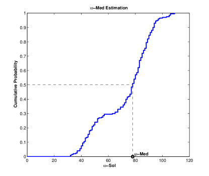
Figure 2: $\omega$-median Approximation

IV-B Convergence of $\omega$-median in $M$

The convergence of the $\omega$-median in the number of sample-paths $M$ is shown in Figure 3, in which $M$ varies from 10 to 1000 in increments of 10. It can be seen that the estimate of the $\omega$-median quickly converges within $100$ replications, which supports the result in Theorem 2.

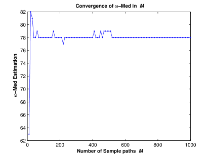
Figure 3: Convergence of $\omega$-median in $M$

IV-C Stationary Cases: “Optimality in Expectation” vs. “Optimality in Probability”

The optimal static policies $(s^{\ast},S^{\ast})$ have been exactly derived by using the algorithm in [20] for stationary cases with different $\mu$. This provides an opportunity to benchmark the performance of the champion solution against the optimal policy $(s^{\ast},S^{\ast})$, the best solution in the sense of “optimality in expectation”.

We set $\mu=20$ in the following experiment, in which 20 instances with $N=50$ periods are randomly generated, and we compare the two methods below:

1. Method SS: Order decisions are directly obtained according to the optimal static policy $(s^{*}=14,S^{*}=62)$ as obtained in [20];

2. Method CS: Order decisions are obtained by using the $\omega$-median approximation with $M=100$ sample paths at the beginning of each period, namely, the estimates of champion solutions.

The performance comparison results are listed in Table II, in which the first column is the instance index, the second column is the cost $C_{ss}$ of using method SS, the third column is the cost $C_{cs}$ of using method CS, the fourth column is the difference between the two costs and the fifth column is the fractional improvement defined as $\frac{(C_{cs}-C_{ss})}{C_{ss}}$.

TABLE II: Stationary Demands

	Cost of SS	Cost of CS	Difference	Improvement
	$C_{ss}$	$C_{cs}$	$C_{ss}-C_{cs}$	$\frac{(C_{cs}-C_{ss})}{C_{ss}}$
1	2401	2439	-38	-1.58%
2	2710	2590	120	4.43%
3	2525	2561	-36	-1.43%
4	2612	2574	38	1.45%
5	2450	2700	-250	-10.20%
6	2390	2724	-334	-13.97%
7	2401	2552	-151	-6.29%
8	2711	2516	195	7.19%
9	2410	2670	-260	-10.79%
10	2598	2454	144	5.54%
11	2563	2559	4	0.16%
12	2441	2570	-129	-5.28%
13	2530	2469	61	2.41%
14	2419	2446	-27	-1.12%
15	2571	2488	83	3.23%
16	2365	2599	-234	-9.89%
17	2622	2542	80	3.05%
18	2672	2502	170	6.36%
19	2480	2372	108	4.35%
20	2543	2608	-65	-2.56%
Mean	2520.7	2546.75	-26.05	-1.03%

From Table II, the average operating cost of SS is slightly less than the one of CS, which confirms that the order decisions based on the optimal policy $(s^{*},S^{*})$ are truly the best in the sense of optimality in expectation.

We can also observe that the order decisions based on the estimated champion solutions perform better than the ones based on the optimal policy $(s^{*},S^{*})$ in 10 instances, i.e., instances 2, 4, 8, 10, 11, 13, 15, 17, 18 and 19. CS has a winning ratio of $50\%$ against SS based on these 20 instances, which implies that the estimated champion solutions perform as well as the exact optimal policy in the sense of optimality in probability in this numerical experiment. Besides, the estimated champion solutions are not the exact champion solutions and we can further improve the performance by increasing the sample size $M$.

Even though decision makers may prefer the sense of optimality in expectation, the estimated champion solutions are near-optimal, since their corresponding average cost is only $1.03\%$ worse than the one of the optimal policy in expectation.

IV-D Nonstationary Cases

In the following experiments of nonstationary cases, we set different $\mu_{i}$ for each period, which are randomly selected from the values listed in $\{10,15,20,...,70,75\}$.

TABLE III: Nonstationary Demands

	Cost of SS	Cost of CS	Difference	Improvement
	$C_{ss}$	$C_{cs}$	$C_{ss}-C_{cs}$	$\frac{(C_{ss}-C_{cs})}{C_{ss}}$
1	3506	2908	598	17.06%
2	3642	2938	704	19.33%
3	3467	3073	394	11.36%
4	3611	3022	589	16.31%
5	3540	3004	536	15.14%
6	3519	3092	427	12.13%
7	3516	3033	483	13.74%
8	3782	3096	686	18.14%
9	3440	2989	451	13.11%
10	3567	2907	660	18.50%
11	3846	2992	854	22.20%
12	3251	2918	333	10.24%
13	3388	2750	638	18.83%
14	2990	2807	183	6.12%
15	3434	2868	566	16.48%
16	3633	3167	466	12.83%
17	3643	2984	659	18.09%
18	3535	3038	497	14.06%
19	3456	3192	264	7.64%
20	3251	3071	180	5.54%
Mean	3500.85	2992.45	508.4	14.52%

We again generate 20 instances with $N=50$ periods and compare two methods below:

1. Method SS: Order decisions are directly obtained according to a heuristic nonstationary policy $(s_{i},S_{i})$ for each period $i$. A common heuristic method is to determine $(s_{i},S_{i})$ according to $\mu_{i}$ in the corresponding period $i$ as if demands are stationary with the mean value of $\mu_{i}$. For example, if $\mu_{1}=15,\mu_{2}=30,\mu_{3}=20,...$, then we can look up the table obtained in [20] to find their corresponding optimal values, choose $(s_{1}=10,S_{1}=49)$, $(s_{2}=23,S_{2}=66)$, $(s_{3}=14,S_{3}=62),...,$ to apply in period $1,2,3,...,$ respectively. Clearly, this heuristic $(s_{i},S_{i})$ policy is not optimal for the nonstationary case.

2. Method CS: Order decisions are still obtained by using the $\omega$-median approximation with $M=100$ sample paths at the beginning of each period, namely, the estimates of champion solutions.

The performance comparison results are listed in Table III that shares a similar organization with Table II. It can be easily seen that the estimated champion solutions result in a $14.52\%$ lower average cost and perform better than the heuristic $(s_{i},S_{i})$ policy in all 20 instances.

V Conclusion

An alternate optimality sense, optimality in probability, is proposed in this paper. The best solution using optimality in probability is termed a “Champion Solution” whose actual performance is more likely better than that of any other solution. A sufficient existence condition for the champion solution is proved for a class of simulation-based optimization problems. A highly efficient method, the Omega Median Algorithm (OMA), is developed to compute the champion solution without iteratively exploring better solutions based on sample average approximations. OMA can reduce the computational complexity by orders of magnitude compared to general simulation-based optimization methods using optimality in expectation.

The champion solution becomes particularly meaningful when facing a nonstationary environment. As shown in the example of inventory control with nonstationary demand, the solution using optimality in expectation is not necessarily optimal and is computationally intractable in a dynamic environment. The champion solution is a good alternative and computationally promising. Its corresponding solution algorithm, OMA, can fully utilize the efficiency of those well-developed off-line algorithms to further facilitate timely decision making, which is preferable in a dynamic environment with limited computing resources. Moreover, even for some stationary scenarios as shown in the numerical results, the “Champion Solution” can still achieve a performance comparable to the one using optimality in expectation.

Future work is aiming at generalizing the sufficient existence condition and extending the idea of champion solution to a wider class of stochastic optimization problems.

References

- [1] Kenneth J. Arrow. Social Choice and Individual Values. Yale University Press, 1963.
- [2] R. G. Askin. A procedure for production lot sizing with probabilistic dynamic demand. AIIE Transactions, 12(2):132–137, 1981.
- [3] S. Axsäter. Inventory Control (Second Edition). Springer, 2006.
- [4] D. P. Bertsekas. Dynamic Programming and Optimal Control Vol.1 (Second Edition). Athena Scientific, 2000.
- [5] Srinivas Bollapragada and Thomas E. Morton. A simple heuristic for computing nonstationary (s,S) policies. Operations Research, 47(4):576–584, 1999.
- [6] C. G. Cassandras, Y. Wardi, B. Melamed, G. Sun, and C. G. Panayiotou. Perturbation analysis for on-line control and optimization of stochastic fluid models. IEEE Trans. on Automatic Control, 47(8):1234–1248, 2002.
- [7] C. H. Chen and L. H. Lee. Stochastic Simulation Optimization: An Optimal Computing Budget Allocation. World Scientific Publishing Co., 2011.
- [8] H. Chen. Stochastic Root Finding in System Design. Ph.D. Thesis. Purdue University, West Lafayette, Indiana, USA., 1994.
- [9] E. K. P. Chong, R. L. Givan, and H. S. Chang. A framework for simulation-based network control via hindsight optimization. In Proceedings of the 39th IEEE Conference on Decision and Control, pages 1433–1438, 2000.
- [10] AWI Federgruen and Michal Tzur. The dynamic lot-sizing model with backlogging: A simple algorithm and minimal forecast horizon procedure. Naval Research LOgistics, 40(4):459–478, 1993.
- [11] Y. C. Ho and X. R. Cao. Perturbation Analysis of Discrete-Event Dynamic Systems. Kluwer Academic Publisher, Boston, 1991.
- [12] Yu-Chi Ho, Qian-Chuan Zhao, and Qing-Shan Jia. Ordinal Optimization: Soft Optimization for Hard Problems. Springer Science & Business Media, 2008.
- [13] W. Hoeffding. Probability inequalities for sums of bounded random variables. Journal of the American Statistical Association, 58(301):13–30, March 1963.
- [14] L. Jeff Hong and Barry L. Nelson. Discrete optimization via simulation using compass. Operations Research, 54(1):115–129, 2006.
- [15] J. Jin. Simulation-Based Retrospective Optimization of Stochastic Systems. Ph.D. Thesis. Purdue University, West Lafayette, Indiana, USA., 1998.
- [16] J. Mao and C. G. Cassandras. On-line optimal control of a class of discrete event systems with real-time constraints. Journal of Discrete Event Dynamic Systems, 20(2):187–213, 2010.
- [17] L. Shi and S. Olafsson. Nested partitions method for global optimization. Operations Research, 48(3):390–407, 2000.
- [18] G. Wu, E. K. P. Chong, and R. L. Givan. Burst-level congestion control using hindsight optimization. IEEE Transactions on Automatic Control, special issue on Systems and Control Methods for Communication Networks, 47(6):979–991, 2002.
- [19] Chen Yao and C. G. Cassandras. A solution to the optimal lot sizing problem as a stochastic resource contention game. IEEE Trans. on Automation Science and Engineering, 9(2):250–264, 2012.
- [20] Y. Zheng and A. Federgruen. Finding optimal (s,S) policies is about as simple as evaluating a single policy. Operations Research, 39(4):654–665, 1991.
- [21] Y. S. Zheng. A simple proof for optimality of (s,S) policies in infinite-horizon inventory systems. Journal of Applied Probability, 28:802–810, 1991.