Theory for Reliable First-Principles Prediction of the Superconducting Transition Temperature

Abstract

A review is given for the theoretical framework to give a reliable prediction of the superconducting transition temperature $T_{c}$ from first principles, together with a practical strategy for its application to actual materials with illustrations of the results of $T_{c}$ calculated for superconductors in the weak-coupling region like the alkali and alkaline-earth intercalated graphites as well as those in the strong-coupling region like the alkali-doped fullerides.

I Introduction

In quantum mechanics, a ground state is determined through a compromise between the kinetic energy (which makes particles itinerant) and the potential energy (which makes them localized). If the latter includes the interaction between particles, there appears a further complication due to their correlated motion. In elucidating the microscopic mechanism of superconductivity, this intrinsic complexity in quantum mechanics cannot be avoided but is even more intensified, specifically because superconductivity is a phenomenon in which an assembly of electrons, negatively charged particles with one-half spin, goes into the pair-condensed phase as a consequence of the dominance of some effective attractions between electrons mediated by either phonons, plasmons, spin-fluctuations, or orbital-fluctuations over the short-range Coulomb repulsions, indicating the necessity of deeply understanding and carefully investigating the physics of this charge-spin-phonon(-orbital) complex before making a reliable evaluation of the transition temperature $T_{c}$ of this second-order phase transition. Thus one would imagine that the task of reliably calculating $T_{c}$ must be formidably difficult, but the ultimate goal in the theoretical study of high-$T_{c}$ superconductivity should be to construct a good theoretical framework for an accurate prediction of $T_{c}$; without such a theoretical tool, we could never conduct a research directly and intimately touched with the most salient feature of high-$T_{c}$ materials, namely, the very feature that $T_{c}$ becomes very high in those materials.

McMillan was the first to provide a rather successful scheme for predicting $T_{c}$ in the phonon mechanism of superconductivity, starting from the microscopic electron-phonon coupled Hamiltonian. The scheme is known as the McMillan’s formula McMillan68 , which was revised later by Allen and Dynes Allen75 ; Allen82 ; Carbotte90 . The formulae, both original and revised, are derived from the Eliashberg theory of superconductivity Eliashberg60 and the task of a microscopic calculation of $T_{c}$ in this framework is reduced to the evaluation of the so-called Eliashberg function $\alpha^{2}F(\omega)$ from the first-principles Hamiltonian, where $F(\omega)$ is the phonon density of states which may be observed by neutron diffraction. This function $\alpha^{2}F(\omega)$ enables us to obtain both the nondimensional electron-phonon coupling constant $\lambda$ and the average phonon energy $\omega_{0}$, through which we can give a first-principles prediction of $T_{c}$ with an additional introduction of a phenomenological parameter $\mu^{*}$ (the Coulomb pseudopotential Morel62 ) for the purpose of roughly estimating the effect of the short-range Coulomb repulsion between electrons on $T_{c}$.

At present, this framework is usually regarded as the standard one for making a first-principles prediction of $T_{c}$ and widely used. In fact, the superconducting mechanism of many (so-called weakly-correlated) superconductors is believed to be clarified by employing this scheme. The key phonon modes to bring about superconductivity are identified by investigating the structure of $\alpha^{2}F(\omega)$. We can mention that superconductivity in MgB₂ with $T_{c}=39$K provides a very good example Bohnen01 ; Kong01 ; Choi02a ; Choi02b to illustrate the power of this scheme. The case of CaC₆ with $T_{c}=11.5$K seems to constitute another recent example Mazin ; Mauri .

In spite of these and many other successful examples, however, this is not considered to be our ultimate scheme for calculating $T_{c}$ from first principles, primarily because a phenomenological parameter $\mu^{*}$ is included in the theory. Actually, it cannot be regarded as the method of predicting $T_{c}$ in the true sense of the word, if the parameter $\mu^{*}$ is determined so as to reproduce the observed $T_{c}$. Besides, as long as $\mu^{*}$ is employed to avoid a serious investigation of the effects of the Coulomb repulsion on superconductivity, this scheme cannot be applied to strongly-correlated superconductors such as the high-$T_{c}$ cuprates. Even in weakly- or moderately-correlated superconductors, this scheme cannot treat superconductivity originating from the Coulomb repulsion via charge, spin, and/or orbital fluctuations (namely, the electronic mechanism including the plasmon mechanism Takada78 ; Takada93a ). Furthermore, in this scheme, we cannot investigate the competition or the coexistence (or even the mutual enhancement due to the quantum-mechanical constructive interference effect) between the phonon and the electronic mechanisms.

The validity of the concept of $\mu^{*}$ is closely related to that of the Eliashberg theory itself; the theory is valid only if the Fermi energy of the superconducting electronic system, $E_{\rm F}$, is much larger than $\omega_{0}$. Note that under the condition of $E_{\rm F}\gg\omega_{0}$, the dynamical response time for the phonon-mediated attraction $\omega_{0}^{-1}$ is much slower than that for the Coulomb repulsion $E_{\rm F}^{-1}$, precluding any possible interference effects between two interactions, so that physically it is very plausible to separate them. After this separation, the Coulomb part (which was not anticipated to play a positive role in the Cooper-pair formation) has been simply treated in terms of a single parameter $\mu^{*}$. Thus, for the purpose of searching for some positive role of the Coulomb repulsion in superconductivity, the concept of $\mu^{*}$ is irrelevant from the outset of the whole theory.

As for the condition of $E_{\rm F}\gg\omega_{0}$, it must also be noted that such a condition is violated in some recently discovered superconductors in the phonon mechanism including the alkali-doped fullerenes with $T_{c}=18-38$K Hebard91 ; Takabayashi09 ; Gunnarsson97 ; Takada98 . Once it is violated, we need to include higher-order corrections in the electron-phonon coupling (or the so-called vertex corrections $\Gamma$) in calculating the phonon-mediated attractive interaction Takada93b . Then, it is by no means clear whether we can fully treat the overall effect of various phonons in terms of the sum of the contribution from each phonon. This implies that the Eliashberg function $\alpha^{2}F(\omega)$ will not be appropriate enough to describe the phonon-mediated attraction because of possible interference effects among virtually-excited different phonon modes. As a consequence, $\lambda$ will not be simply the sum of $\lambda_{i}$ the contribution from the $i$th phonon, unless $\lambda_{i}$ is small enough to validate the whole calculation in lowest-order perturbation.

If the condition of $E_{\rm F}\gg\omega_{0}$ is violated, especially if $E_{\rm F}$ is about the same as $\omega_{0}$, another complication occurs in treating the screening effect of the conduction electrons. In the usual calculation scheme from first principles, the static screening is assumed in calculating $\alpha^{2}F(\omega)$, but it does not reflect the actual screening process working during the formation of Cooper pairs. This subtle problem of screening is, of course, also closely related to the problem of the first-principles determination of $\mu^{*}$ and we will not be able to solve these problems unambiguously without confronting with a difficult task of treating both the Coulomb repulsion and the phonon-mediated attraction on the same footing in the calculation of the microscopic dynamical electron-electron effective interaction $V$.

In order to overcome the above-mentioned problems inherently associated with the Eliashberg theory, the first and natural option would be to improve on it by considering both the gap equation and the electron-electron effective interaction $V$ in entire energy- and momentum-space with properly including the vertex corrections $\Gamma$ in $V$ and without separating the Coulomb repulsion from $V$. However, this will not be easily accomplished at least in the near future, partly because the demand for computational resources becomes too much in the solution of the full nonlocal and dynamical gap equation and partly because no controlled approximation scheme has been known for $\Gamma$ for the superconducting state. (Note that the controlled scheme is known for the normal state Takada95 ; Takada01 .)

Fortunately, an alternative option has already been proposed by the extension of the density functional theory (DFT) to treating a superconducting state Oliveira88 ; Kurth99 . This theory provides a formally exact framework for calcualting $T_{c}$ from first principles by the solution of the gap equation only in momentum-space, setting aside the calculation of other physical quantities except for the one-electron density $n({\bm{r}})$. Note that the effect of the Coulomb repulsion is properly included in this formulation without resort to the concept of $\mu^{*}$. Therefore we shall begin with making a very brief review of this density fuctional theory for superconductors (SCDFT) in Sec. II. We shall point out that the central quantity in this framework is the pairing interaction ${\cal K}$. Then in Sec. III, we shall infer a concrete formula for ${\cal K}$ defined in terms of the Kohn-Sham orbitals in an inhomogeneous electron gas by reconsidering the gap equation for the homogeneous electron gas in the weak-coupling region with use of the Green’s-function method. The formula has not been proposed so far in the literature in SCDFT, but by its application to superconductivity in the alkali- and alkaline-earth intercalated graphites Takada09a ; Takada09b , it turns out that this is indeed a very good approximate functional form for ${\cal K}$. A prediction for the optimum value of $T_{c}$ by using this functional form will be given for this class of materials. In Sec. IV, we shall consider a formula for ${\cal K}$ in the opposite limit, namely, in the strong-coupling region, especially for such superconductors with short coherence lengths as the alkali-doped fullerides Takada07 . By interpolating the formulae for ${\cal K}$ in these two limits, we shall propose a new functional form for ${\cal K}$ which is supposed to work well in the whole range of the coupling strength. The results of $T_{c}$ obtained by its application to the fullerene superconductors and related materials will be shown in the last subsection of this section. Finally in Sec. V we shall conclude this short article, together with discussing the direction of future research.

II Density Functional Theory for Superconductors (SCDFT)

II.1 Hohenberg-Kohn-Sham Theorem

According to the basic theorem in the density functional theory (DFT) due to Hohenberg and Kohn Hohenberg64 , all the physical quantities of an interacting electron system are uniquely determined, once its electronic density in the ground state $n({\bm{r}})$ is specified. This implies that every quantity including the exchange-correlation energy $F_{xc}$ may be considered as a unique functional of $n({\bm{r}})$. The ground-state density $n({\bm{r}})$ itself can be determined by the calculation of the ground-state electronic density of the corresponding noninteracting reference system that is stipulated in terms of the Kohn-Sham (KS) equation Kohn65 . The concept of the noninteracting reference system is of central importance in the KS algorithm and the core quantity in the KS equation is the exchange-correlation potential $V_{xc}({\bm{r}})$, which is formally defined as the first-order functional derivative of $F_{xc}[n({\bm{r}})]$ with respect to $n({\bm{r}})$, namely, $V_{xc}({\bm{r}})=\delta F_{xc}[n]/\delta n({\bm{r}})$. It must be noted that $V_{xc}({\bm{r}})$ as well as each one-electronic wavefunction at $i$th level (usually called as “$i$th KS orbital”) with its energy eigenvalue $\varepsilon_{i}$ in the KS equation has no direct physical relevance; they are merely introduced for the mathematical convenience so as to obtain the exact $n({\bm{r}})$ in the real many-electron system by exploitation of its one-to-one correspondence to the noninteracting reference system.

This basic Hohenberg-Kohn theorem can be applied not only to the normal ground state but also to the ordered one on the understanding that the order parameter itself in the ordered state is regarded as a functional of $n({\bm{r}})$. In providing some approximate functional form for $F_{xc}[n]$ in actual calculations, however, it would be more convenient to treat the order parameter as an additional independent variable. For example, in considering the system with a collinear magnetic order, we usually employ the spin-dependent scheme in which the fundamental variable is not $n({\bm{r}})$ but the spin-decomposed density $n_{\sigma}({\bm{r}})$, leading to the spin-polarized exchange-correlation energy functional $F_{xc}[n_{\sigma}]$, based on which the spin-dependent exchange-correlation potential is defined to specify the spin-dependent KS equation for determining $n_{\sigma}({\bm{r}})$ from first principles.

II.2 Gap Equation in SCDFT

In an essentially similar way, in treating superconductivity in the framework of DFT, it would be better to construct the energy functional with employing both $n({\bm{r}})$ and the electron-pair density (or the superconducting order parameter) $\chi({\bm{r}},{\bm{r}^{\prime}})(\equiv\langle\Psi_{\uparrow}({\bm{r}})\Psi_{\downarrow}({\bm{r}^{\prime}})\rangle)$ as basic variables Oliveira88 ; Kurth99 , leading to the pair-density-dependent exchange-correlation energy functional $F_{xc}[n({\bm{r}}),\chi({\bm{r},r^{\prime}})]$, where $\Psi_{\sigma}({\bm{r}})$ is the annihilation operator of $\sigma$-spin electron field at position ${\bm{r}}$. In accordance with this addition of the order parameter as a fundamental variable to DFT, not only the exchange-correlation potential $V_{xc}({\bm{r}})$ but also the exchange-correlation pair-potential $\Delta_{xc}({\bm{r}},{\bm{r}^{\prime}})=-\delta F_{xc}[n,\chi]/\delta\chi^{*}({\bm{r}},{\bm{r}^{\prime}})$ appear in an extended KS equation. A beautiful point in this density functional theory for superconductors (SCDFT) is that the extended KS equation can be written in the form of the Bogoliubov-de Gennes equation appearing in the conventional theory for inhomogeneous superconductors deGennes66 . Just as is the case with $V_{xc}({\bm{r}})$, $\Delta_{xc}({\bm{r}},{\bm{r}^{\prime}})$ has no direct physical meaning, but in principle, if the exact form of $F_{xc}[n,\chi]$ is known, the solution of the extended KS equation gives us the exact result for $\chi({\bm{r}},{\bm{r}^{\prime}})$, containing all the effects of the Coulomb repulsion including the one usually treated phenomenologically through the concept of $\mu^{*}$. As a result, we can determine the exact $T_{c}$ by the calculation of the highest temperature below which a nonzero solution for $\chi({\bm{r}},{\bm{r}^{\prime}})$ can be found.

In this framework of SCDFT, we can formally write down the fundamental gap equation to determine $T_{c}$ exactly as Units-here

$$\Delta_{j}=-\sum_{j^{\prime}}{\Delta_{j^{\prime}}\over 2\varepsilon_{j^{\prime}}}\tanh{\varepsilon_{j^{\prime}}\over 2T_{c}}\,{\cal K}_{jj^{\prime}},$$ (1)

where $\Delta_{j}$ is the gap function associated with $j$th KS orbital. In just the same way as its energy eigenvalue $\varepsilon_{j}$ (which is measured relative to the chemical potential), $\Delta_{j}$ is not the quantity to be observed experimentally but just introduced for the mathematical convenience so as to obtain the exact $T_{c}$ by solving this BCS-type equation, Eq. (1). Similarly, the pairing interaction ${\cal K}_{jj^{\prime}}$, defined as the second-order functional derivative of $F_{xc}[n,\chi]$ with respect to $\chi^{*}$ and $\chi$, has not any direct physical meaning, either, although this is a quantity of primary importance in this gap equation or even in the whole framework of SCDFT.

Three comments are in order: (i) The functional derivatives of $F_{xc}[n,\chi]$ might not be well defined, as anticipated by remembering the notorious energy-gap problem in semiconductors and insulators Perdew83 ; Sham83 ; Sham85 , but as is ordinally the case, we shall assume that ${\cal K}_{jj^{\prime}}$ is a well-defined quantity. (ii) In this formal derivation in SCDFT, the dynamical (or $\omega$-dependent) nature in the electron-electron multiple scatterings does not manifest itself in either the gap equation or the pairing interaction, in sharp contrast with the Eliashberg theory. For this reason, many people cast doubt on whether the physics leading to $\mu^{*}$ is actually taken into account in SCDFT. However, due to the fact that there is a very good correspondence between this gap equation and the one in the $G_{0}W_{0}$ approximation to the Elishaberg theory, as will be shown in the next section, we find that it is possible to include the full dynamical processes in the Cooper-pair formation in the framework of SCDFT, as long as the form of ${\cal K}_{jj^{\prime}}$ is properly chosen. (iii) At $T=T_{c}$, ${\cal K}_{jj^{\prime}}$ is evaluated at $\chi=0$. Thus ${\cal K}_{jj^{\prime}}$ must be a functional of only the normal-state electronic density $n({\bm{r}})$. Note that each KS orbital, $j$ or $j^{\prime}$, determined in the normal state may be regarded as a functional of $n({\bm{r}})$, justifying the view that ${\cal K}_{jj^{\prime}}$ at $T=T_{c}$ is eventually a functional of $n({\bm{r}})$ in the normal state.

II.3 Application and Discussion

This formal framework of SCDFT was not applied to actual superconductors before the year 2005 when an attempt was made to provide a concrete approximate form for $F_{xc}[n,\chi]$ in which the contribution from the phonon-mediated attraction was explicitly included up to the level of the Eliashberg theory Luders05 . Since then many (but mostly weakly-correlated) superconductors have been analyzed rather successfully in this framework Sanna07 ; Marques05 ; Floris05 ; Profeta06 ; Sanna06 ; Floris07 .

In the judgement of the present author, the presently available form for $F_{xc}[n,\chi]$ or the one for ${\cal K}_{jj^{\prime}}$ contains the information equivalent to that included in the Eliashberg theory for the part of the phonon-mediated attraction, indicating that no vertex corrections are considered in this treatment (amounting to the very insufficient treatment of the strong polaronic effect), while for the part of the Coulomb repulsion, it contains only very crude physics; the screening effect is treated in the Thomas-Fermi static-screening approximation, or the result in the random phase approximation (RPA) only in the static and the long-wavelength limit, neglecting both the dynamical and nonlocal feature in the effects of the Coulomb repulsion. This clearly indicates that the Coulomb repulsion is not treated on the same footing as the phonon-mediated attraction and this approximation for the Coulomb part will be just good for describing the physics represented by $\mu^{*}$ at usual metallic densities (or $r_{s}\approx 2$ with $r_{s}$ the conventional nondimensional density parameter) from first principles, but it fails to take care of the detailed dynamical nature of the screening effect, especially, the positive role of the plasmons in superconductivity for lower densities (or larger $r_{s}$) Takada78 ; Takada93a . Furthermore, the presently available form for $F_{xc}[n,\chi]$ or ${\cal K}_{jj^{\prime}}$ does not allow to discuss other types of the electronic mechanisms such as the spin-fluctuation one, either. In view of these fundamental problems, it is absolutely necessary to derive a much better approximate functional form for ${\cal K}_{jj^{\prime}}$ for the purpose of investigating the electronic mechanisms in the absence/presence of the phonon mechanism.

It would be appropriate here to make a rather general comment on numerical errors. Currently, calculations of the normal-state properties are done in either the local-density approximation (LDA) or the generalized gradient approximation (GGA) Perdew96 to $F_{xc}[n({\bm{r}})]$ in DFT. We usually anticipate that errors in the calculated results are of the order of 1eV and 0.3eV for LDA and GGA, respectively, and those errors are much larger than that expected in quantum chemistry ($\approx 0.05$eV). Now in the usual procedure in SCDFT, the calculation of $T_{c}$ (which is of the order of 0.001eV in general) is done simultaneously with that of the normal state and thus the error for $T_{c}$ might be of the same order as that for the normal-state properties, implying that it might become much larger than $T_{c}$ itself.

This unfavorable situation may be avoided, if we take the following two-stage strategy for the calculation of $T_{c}$ for a family of superconducting materials in consideration; in the first stage, combined with available experimental results on the normal state, we establish a good model system representing this family of superconductors by making a first-principles band-structure calculation and then in the second stage, we evaluate $T_{c}$ based on the model system not only for reproducing the experimental $T_{c}$ but also for suggesting not yet synthesized but promising superconductors with higher $T_{c}$ in this family. In the rest of this article, we shall discuss two families of the carbon-based superconductors for which $T_{c}$s are calculated and predicted in accordance with this two-stage strategy.

III G₀W₀ Approximation with Application to Graphite Intercalation Compounds

III.1 Pairing Interaction in the Weak-Coupling Region

The three-dimensional (3D) homogeneous electron gas has been known to be a very useful system in constructing a successful functional form for $V_{xc}({\bm{r}})$ in either LDA or GGA by its study with use of various powerful many-body techniques including quantum Monte Carlo simulations. In view of this success, we shall study superconductivity in the same system with the conventional Green’s-function method in order to infer a good functional form for the pairing interaction ${\cal K}_{jj^{\prime}}$ in Eq. (1) that will be exact in the weak-coupling limit.

In a homogeneous system, momentum ${\bm{p}}$ is always a good quantum number and an electron can be specified by ${\bm{p}}$ and spin $\sigma$. If we write the electron annihilation operator by $c_{{\bm{p}}\sigma}$, the Hamiltonian $H$ of the 3D electron-gas system coupled with phonons is given by

$$H= H_{e}+H_{ph}$$

$$= \sum_{{\bm{p}}\sigma}\varepsilon_{\bm{p}}c_{{\bm{p}}\sigma}^{+}c_{{\bm{p}}\sigma}$$

$$+{1\over 2}\sum_{{\bm{q}}\neq{\bm{0}}}\sum_{{\bm{p}}\sigma}\sum_{{\bm{p}^{\prime}}\sigma^{\prime}}V_{0}({\bm{q}})c_{{\bm{p}}\sigma}^{+}c_{{\bm{p}^{\prime}}\sigma^{\prime}}^{+}c_{{\bm{p}^{\prime}-q}\sigma}c_{{\bm{p}+q}\sigma^{\prime}}$$

$$+H_{ph},$$ (2)

where $\varepsilon_{\bm{p}}\ (\equiv{\bm{p}}^{2}/2m^{*}\!-\!\mu)$ is the bare one-electron dispersion relation with $m^{*}$ the band mass and $\mu$ the chemical potential, $V_{0}({\bm{q}})\ (\equiv 4\pi e^{2}/\epsilon_{\infty}{\bm{q}}^{2})$ is the bare Coulomb repulsion with $\epsilon_{\infty}$ the optical dielectric constant, and $H_{ph}$ represents all contributions containing the phonon operators. For the time being, there is no need of our specifying a concrete form for $H_{ph}$.

In the thermal Green’s-function method, we can treat superconductivity by introducing the abnormal thermal Green’s function $F({\bm{p}},i\omega_{p})$, which is defined at temperature $T$ by

$$F({\bm{p}},i\omega_{p})=-\int_{0}^{1/T}\!d\tau\,e^{i\omega_{p}\tau}\langle T_{\tau}c_{{\bm{p}}\uparrow}(\tau)c_{-{\bm{p}}\downarrow}\rangle.$$ (3)

Here $\omega_{p}$ is the fermion Matsubara frequency, defined by $\pi T(2p+1)$ with an integer $p$. At $T=T_{c}$ where the second-order superconducting phase transition occurs, this function satisfies the following formally exact gap equation:

$$F({\bm{p}},i\omega_{p})\!=\! -G({\bm{p}},i\omega_{p})G(-{\bm{p}},-i\omega_{p})$$

$$\times T_{c}\!\sum_{\omega_{p^{\prime}}}\!\sum_{\bm{p}^{\prime}}\!\tilde{J}({\bm{p},p^{\prime}};i\omega_{p},i\omega_{p^{\prime}})F({\bm{p}^{\prime}},i\omega_{p^{\prime}}),$$ (4)

where $G({\bm{p}},i\omega_{p})$ is the normal thermal Green’s function and $\tilde{J}({\bm{p}},{\bm{p}^{\prime}};i\omega_{p},i\omega_{p^{\prime}})$ is the irreducible electron-electron effective interaction.

Let us assume that the effect of interaction is weak, so that it would be enough to retain the terms only in lowest order in the interaction. If we adopt the same assumption in the calculation of the normal-state properties in the Green’s-function approach, we are led to the so-called $G_{0}W_{0}$ approximation or the one-shot $GW$ approximation in terminology prevailing in the present-day first-principles calculation community, where $W$ is the effective interaction between electrons including both the Coulomb and the phonon-mediated interactions and $W_{0}$ represents $W$ in RPA. Incidentally, in the same kind of terminology, the Eliashberg theory corresponds to the $GW$ approximation. Historically, Cohen was the first to evaluate $T_{c}$ in degenerate semiconductors on the level of the $G_{0}W_{0}$ approximation Cohen64 ; Cohen69 . Unfortunately the pairing interaction is not correctly derived in his theory, as explicitly pointed out by the present author Takada80 who, instead, by consulting the pertinent work of Kirzhnits et al. Kirzhnits73 , has succeeded in obtaining the correct pairing interaction Takada78 , the result of which will be reiterated in the following.

In the $G_{0}W_{0}$ approximation, we replace $G({\bm{p}},i\omega_{p})$ by the bare one $G_{0}({\bm{p}},i\omega_{p})\ [\equiv(i\omega_{p}\!-\!\varepsilon_{\bm{p}})^{-1}]$ in Eq. (4) and consider the case in which $\tilde{J}({\bm{p},p^{\prime}};i\omega_{p},i\omega_{p^{\prime}})$ is well approximated as a function of only the variables, ${\bm{p}}\!-\!{\bm{p}^{\prime}}$ and $i\omega_{p}\!-\!i\omega_{p^{\prime}}$, to write

$$\tilde{J}({\bm{p}},{\bm{p}^{\prime}};i\omega_{p},i\omega_{p^{\prime}})=V({\bm{p}}\!-\!{\bm{p}^{\prime}},i\omega_{p}\!-\!i\omega_{p^{\prime}}),$$ (5)

as is usually the case for $W_{0}$ the effective interaction in RPA, though we do not intend to confine ourselves to RPA at this stage. By substituting Eq. (5) into Eq. (4), we obtain the gap equation in the $G_{0}W_{0}$ approximation as

$$F({\bm{p}},i\omega_{p})\! =\!-\!G_{0}({\bm{p}},i\omega_{p})G_{0}(-\!{\bm{p}},-\!i\omega_{p})$$

$$\times\!T_{c}\!\sum_{\omega_{p^{\prime}}}\!\sum_{\bm{p}^{\prime}}\!V({\bm{p}}\!-\!{\bm{p}^{\prime}},i\omega_{p}\!-\!i\omega_{p^{\prime}})\!F({\bm{p}^{\prime}},i\omega_{p^{\prime}}).$$ (6)

Then, by making an analytic continuation on the $\omega$ plane to transform $F({\bm{p}},i\omega_{p})$ to the retarded function $F^{R}({\bm{p}},\omega)$ on the real-$\omega$ axis and using the general relation due to the causality principle as

$$V^{R}({\bm{q}},\omega)=V_{0}({\bm{q}})\!-\!\int_{0}^{\infty}\!\frac{d\Omega}{\pi}\frac{2\Omega}{\omega^{2}\!-\!\Omega^{2}+i\eta}\,{\rm Im}V^{R}({\bm{q}},\Omega),$$ (7)

with $\eta$ a positive infinitesimal, we end up with a gap equation for $F^{R}({\bm{p}},\omega)$. Finally, by taking the imaginary parts in both sides of the gap equation and integrating over the $\omega$ variable, we are led to an equation depending only on the momentum variable ${\bm{p}}$. More specifically, the equation can be cast into the following BCS-type gap equation:

$$\Delta_{\bm{p}}=-\sum_{\bm{p}^{\prime}}{\Delta_{\bm{p}^{\prime}}\over 2\varepsilon_{\bm{p}^{\prime}}}\tanh{\varepsilon_{\bm{p}^{\prime}}\over 2T_{c}}\,{\cal K}_{\bm{p},p^{\prime}},$$ (8)

where the gap function $\Delta_{\bm{p}}$ and the pairing interaction ${\cal K}_{\bm{p}},{\bm{p}^{\prime}}$ are, respectively, defined as

$$\Delta_{\bm{p}}\equiv 2|\varepsilon_{\bm{p}}|\int_{0}^{\infty}\!{d\omega\over\pi}\,{\rm Im}\,F^{R}({\bm{p}},\omega),$$ (9)

and

$${\cal K}_{\bm{p}},{\bm{p}^{\prime}} \equiv V_{0}({\bm{p}}-{\bm{p}^{\prime}})\!+\!\int_{0}^{\infty}\!\frac{2}{\pi}\,d\Omega\,\frac{{\rm Im}V^{R}({\bm{p}}-{\bm{p}^{\prime}},\Omega)}{\Omega\!+\!|\varepsilon_{\bm{p}}|\!+\!|\varepsilon_{\bm{p}^{\prime}}|}$$

$$\!=\!\int_{0}^{\infty}\!\frac{2}{\pi}d\Omega\,\frac{|\varepsilon_{\bm{p}}|\!+\!|\varepsilon_{\bm{p}^{\prime}}|}{\Omega^{2}\!+\!(|\varepsilon_{\bm{p}}|\!+\!|\varepsilon_{\bm{p}^{\prime}}|)^{2}}\,V({\bm{p}}\!-\!{\bm{p}^{\prime}},i\Omega).$$ (10)

With use of ${\cal K}_{\bm{p}},{\bm{p}^{\prime}}$ thus derived, we can determine $T_{c}$ as an eigenvalue of Eq. (8), indicating that we have obtained a scheme in which $T_{c}$ is given directly from the microscopic one-electron dispersion relation $\varepsilon_{\bm{p}}$ and the effective electron-electron interaction $V({\bm{q}},i\Omega)$. Because there is no need to separate the phonon-mediated attraction from the Coulomb repulsion in $V({\bm{q}},i\Omega)$ and the dynamical nature of the interaction is fully taken into account, we can properly treat the physics leading to $\mu^{*}$ from first principles with use of this scheme.

The very definition of the gap function $\Delta_{\bm{p}}$ in Eq. (9) indicates that $\Delta_{\bm{p}}$ does not correspond to the physical energy gap except in the weak-coupling limit. Similary, ${\cal K}_{\bm{p}},{\bm{p}^{\prime}}$ is not a physical entity, although $V$ is the physical effective interaction. Both quantities are introduced for the mathematical convenience so as to make $T_{c}$ invariant in transforming Eq. (4) into Eq. (8). The key point here is that we need not solve the full gap equation (4) but much simpler one (8) in order to obtain $T_{c}$ in Eq. (4). Of course, if we want to know the physical gap function rather than $\Delta_{\bm{p}}$ to compare with experiment, we need to solve the full gap equation, Eq. (4), with $T_{c}$ determined by Eq. (8).

Although the spin-singlet pairing has been assumed in the derivation of Eq. (8), no assumption is made on the dependence of the gap function on angular valuables, so that this gap equation can treat any kind of the pairing anisotropy in the gap function, indicating that it can be applied to s-wave, d-wave, $\cdots$, and even their mixture like (s+d)-wave superconductors.

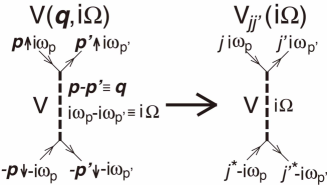
Figure 1: Schematic representation of the dynamical effective interaction $V_{jj^{\prime}}(i\Omega)$ as inferred from $V({\bm{q}},i\Omega)$.

Now, let us compare Eq. (8) with Eq. (1). Since the KS orbitals, $j$ and $j^{\prime}$, can be specified by momenta, ${\bm{p}}$ and ${\bm{p}^{\prime}}$, respectively, in a homogeneous system and $\varepsilon_{j^{\prime}}=\varepsilon_{\bm{p}^{\prime}}$, we may regard that these two equations are esssentially the same, suggesting that we may give a concrete functional form for ${\cal K}_{jj^{\prime}}$ with use of energies of the KS orbitals, $\varepsilon_{j}$ and $\varepsilon_{j^{\prime}}$, as

$${\cal K}_{jj^{\prime}}=\int_{0}^{\infty}\!{2\over\pi}\,d\Omega\,{|\varepsilon_{j}|+|\varepsilon_{j^{\prime}}|\over\Omega^{2}+(|\varepsilon_{j}|+|\varepsilon_{j^{\prime}}|)^{2}}\,V_{jj^{\prime}}(i\Omega)\,.$$ (11)

Here $V_{jj^{\prime}}(i\Omega)$ is the dynamical effective interaction working for the scattering process from a pair of electrons in $(j,j^{*})$ orbitals to another pair in $(j^{\prime},{j^{\prime}}^{*})$ orbitals, as schematically shown in Fig. 1 (By $j^{*}$ we mean the time-reversed KS orbital of $j$.) We should calculate this $V_{jj^{\prime}}(i\Omega)$ on the understanding that it must be derived from the first-principles Hamiltonian expanded with use of a complete set of the KS orbitals as an orthnormal basis. Together with the gap equation, Eq. (1), and the KS orbitals obtained in the normal state by the conventional DFT-based method, Eq. (11) constitutes a basic framework for a first-principles calculation of $T_{c}$ for inhomogeneous weak-coupling superconductors.

III.2 Superconductivity in Polar Semiconductors

In order to assess the quality of this basic framework in the G₀W₀ approximation for calculating $T_{c}$ from first principles, we have applied it to polar degenerate semiconductors, specifically, the doped SrTiO₃ and compared the calculated results with experiments Takada80 .

This material is an insulator and exhibits ferroelectricity under a uniaxial stress of about 0.16GPa along the [100] direction, but it turns into an $n$-type semiconductor by either Nb doping or oxygen deficiency, whereby the conduction electrons are introduced in the 3d band of Ti around the $\Gamma$ point with the band mass of $m^{*}\approx 1.8m_{e}$ ($m_{e}$: the mass of a free electron). At low temperatures, superconductivity appears and the observed $T_{c}$ shows interesting features; $T_{c}$ depends strongly on the electron concentration $n$ and it is optimized with $T_{c}\approx 0.3$K at $n\approx 10^{20}$cm^-3. Its dependence on the pressure is unsual; $T_{c}$ decreases rather rapidly with hydrostatic pressures, but it increases with the [100] uniaxial stress, implying that the superconductivity is brought about by the polar-coupling phonons associated with the stress-induced ferroelectric phase transition,

Taking those situations into account, we have assumed that the material is well represented by a model of the 3D electron-gas system coupled with polar-optical phonons in which a concrete form for $V({\bm{q}},i\Omega)$ can be derived in RPA as

$$V({\bm{q}},i\Omega)={4\pi e^{2}\over\epsilon({\bm{q}},i\Omega)\,{\bm{q}}^{2}},$$ (12)

with the dielectric function in the electron-optical phonon system as

$$\epsilon({\bm{q}},i\Omega)= \epsilon_{\infty}+{4\pi e^{2}\over{\bm{q}}^{2}}\Pi_{0}({\bm{q}},i\Omega)$$

$$+\left[\epsilon_{0}({\bm{q}})-\epsilon_{\infty}\right]{\omega_{t}({\bm{q}})^{2}\over\omega_{t}({\bm{q}})^{2}+\Omega^{2}},$$ (13)

where $\Pi_{0}({\bm{q}},i\Omega)$ is the polarization function in RPA (or the Lindhard function) for the 3D electron gas, $\omega_{t}({\bm{q}})$ is the energy dispersion of the transverse optical phonon, and $\epsilon_{0}({\bm{q}})$ is the static nonlocal dielectric function, which is determined with use of the static dielectric constant $\epsilon_{0}$ and $\omega_{t}({\bm{q}})$ as

$$\epsilon_{0}({\bm{q}})=\epsilon_{0}\,{\omega_{t}(0)^{2}\over\omega_{t}({\bm{q}})^{2}}.$$ (14)

The dispersionless longitudinal-phonon energy $\omega_{\ell}$ is related to the transverse-phonon energy in the long-wavelength limit $\omega_{t}(0)$ through the Lyddane-Sachs-Teller relation as

$$\omega_{\ell}=\sqrt{{\epsilon_{0}\over\epsilon_{\infty}}}\,\omega_{t}(0).$$ (15)

By substituting $V({\bm{q}},i\Omega)$ in Eq. (12) into Eq. (10) and using the experimental data to determine the values of parameters like $\epsilon_{0}$ and $\epsilon_{\infty}$ as well as the dipersion relation for $\omega_{t}({\bm{q}})$, we have obtained $T_{c}$ directly from a microscopic model and the results of $T_{c}$ are in surprizingly good quantitative agreement with experiment, as shown in Fig. 2 The unusual dependence of $T_{c}$ on the pressure is also reproduced well, though it is not shown here. (For interested readers, refer to the original paper Takada80 .) This success indicates that the present framework including the adoption of RPA for calculating the effective interaction is useful and appropriate at least in the polar-coupled phonon mechanism in which the contribution from the long-range part of the interaction dominates over that from the short-range one.

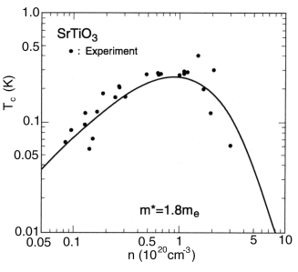
Figure 2: Calculated results for $T_{c}$ in semiconducting SrTiO₃ as a function of the electron density $n$ (the solid curve  Takada80 ), together with the experimental results (the filled circles Koonse . See also Behnia )

III.3 Graphite Intercalation Compounds (GICs)

III.3.1 Historical Survey

The graphite intercalation compounds (GICs) have been investigated for a long time from physical, chemical, and technological points of view PhysToday1 ; PhysToday2 ; Zabel92 ; AdvPhys . Among various kinds of GICs, special attention has been paid to the first-stage metal compounds, mainly because superconductivity is observed only in this class of GICs, the chemical formula of which is written as $M$C_x, where $M$ represents either an alkali atom (such as Li, K, Rb, and Cs) or an alkaline-earth atom (such as Ca, Sr, and Yb) and $x$ is either $2$, $6$, or $8$. The crystal structure of $M$C_x is shown in Fig. 3(a), in which the metal atom $M$ occupies the same spot in the framework of a honeycomb lattice at every $(x/2)$ layers of carbon atoms.

The first discovery of superconductivity in GICs was made in KC₈ with the superconducting transition temperature $T_{c}$ of 0.15K in 1965 Hannay65 . In pursuit of higher $T_{c}$, various GICs were synthesized, mostly working with the alkali metals and alkali-metal amalgams as intercalants, from the late 1970s to the early 1990s Koike78 ; Kobayashi79 ; Koike80 ; Alexander80 ; Iye ; Belash89a ; Dresselhaus89 ; Belash90 , but only a limited success was achieved at that time; the highest attained $T_{c}$ was around 2-5K in the last century. For example, it is 1.9K in LiC₂ Belash89b .

A breakthough occurred in 2005 when $T_{c}$ went up to 11.5K in CaC₆ CaC6 ; Emery (and even to 15.4K under pressures up to 7.5GPa Takagi ). In other alkaline-earth GICs, the values of $T_{c}$ are 6.5K and 1.65K for YbC₆ CaC6 and SrC₆ Kim2 , respectively. Since then, very intensive experimental studies have been made in those and related compounds Emery ; Kim2 ; Kim1 ; Kurter . Theoretical studies have also been performed mainly by making state-of-the-art first-principles calculations of the electron-phonon coupling constant $\lambda$ to account for the observed value of $T_{c}$ for each individual superconductor Mazin ; Csanyi ; Mauri ; Sanna07 . Those experimental/theoretical works have elucidated that, although there are some anisotropic features in the superconducting gap, the conventional phonon-driven mechanism to bring about s-wave superconductivity applies to those compounds. This picture of superconductivity is confirmed by, for example, the observation of the Ca isotope effect with its exponent $\alpha=0.50$, the typical BCS value Hinks .

In spite of all those efforts and the existence of such a generally accepted picture, we need to know more important and fundamental issues that include:

(i) Standard model: Can we understand the mechanism of superconductivity in both alkali GICs with $T_{c}$ in the range $0.01-1.0$K and alkaline-earth GICs with $T_{c}$ in the range $1-10$K from a unified point of view? In other words, is there any standard model for superconductivity in GICs with $T_{c}$ ranging over three orders of magnitude?

(ii) Key parameters to control $T_{c}$: What is the actual reason why $T_{c}$ is enhanced so abruptly (or by about a hundred times) by just substituting K by Ca the atomic mass of which is almost the same as that of K? In terms of the standard model, what are the key controlling physical parameters to bring about this huge enhancement of $T_{c}$? This change of $T_{c}$ from KC₈ to CaC₆ is probably the most important issue in exploring superconductivity across the entire family of GICs.

(iii) Optimum $T_{c}$: Is there any possibility to make a further enhancement of $T_{c}$ in GICs? If possible, what is the optimum value of $T_{c}$ expected in the standard model and what kind of atoms should be intercalated to realize the optimum $T_{c}$ in actual GICs?

Recently these three issues have been satisfactorily addressed by the present author Takada09a ; Takada09b , as shall be explained one by one in the following three subsections.

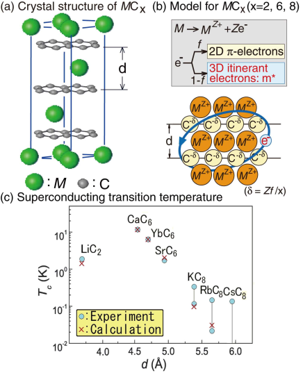
Figure 3: (a) Crystal structure of $M$C_x ($x$=$2,\,6,\,8$). The case of $x$ =$6$ is illustrated here, in which the metal atoms, $M$s, are arranged in a rhombohedral structure with the $\alpha\beta\gamma$ stacking sequence, implying that $M$ occupies the same spot in the framework of a graphene lattice at every three layers (or at the distance of $3d$ with $d$ the distance between the adjacent graphite layers). (b) Simplified model to represent $M$C_x superconductors. We consider the attraction between the 3D electrons in the interlayer band induced by polar-coupled charge fluctuations of the cation $M^{Z+}$ and the anion C^-δ. (c) Superconducting transition temperature $T_{c}$ in the first-stage alkali- and alkaline-earth-intercalated graphites plotted as a function of $d$. The solid circles show the experimental results, while the crosses the calculated ones in the G₀W₀ approximation for the model represented in (b) with suitable values for the parameters such as $Z$, $m^{*}$, and $f$ for each $M$C_x.

III.3.2 Standard Model for Intercalated Graphite Superconductors

The usual DFT-based self-consistent band-structure calculation is useful in elucidating the electronic structures of GICs in the normal state, basically because GICs are not strongly-correlated materials. According to such a calculation, no essential qualitative difference is found between alkali and alkaline-earth GICs. The main common features among these GICs may be summarized as follows:

First of all, each intercalant metal atom in $M$C_x acts as a donor and changes from a neutral atom $M$ to an ion $M^{Z+}$ with valence $Z$. Then, the valence electrons released from $M$ will transfer either to the graphite $\pi$ bands or the three-dimensional (3D) band composed of the intercalant orbitals and the graphite interlayer states Posternak84 ; Holzwarth84 ; Koma86 . We shall define the factor $f$ as the branching ratio between these two kinds of bands. Namely, $Zf$ and $Z(1-f)$ electrons will go to the $\pi$ and the 3D bands, respectively. The electrons in the graphite $\pi$ bands are characterized by the two-dimensional (2D) motion with a linear dispersion relation (known as a Dirac cone in the case of graphene) on the graphite layer.

The dispersion relation of the graphite interlayer band is very similar to that of the 3D free-electron gas, folded into the Brillouin zone of the graphite Csanyi . Thus its energy level is very high above the Fermi level in the graphite, because the amplitude of the wavefunction for this band is small on the carbon atoms. In $M$C_x, on the other hand, the cation $M^{Z+}$ is located in the interlayer position where the amplitude of the wavefunctions is large, lowering the energy level of the interlayer band below the Fermi level. The dispersion of the interlayer band is modified from that of the free-electron gas because of the hybridization with the orbitals associated with $M$, but generally it is well approximated by $\varepsilon_{\bm{p}}={\bm{p}}^{2}/2m^{*}-E_{\rm F}$ with an appropriate choice of the effective band mass $m^{*}$ and the Fermi energy $E_{\rm F}$. Here the value of $m^{*}$ depends on $M$; in alkali GICs, the hybridization occurs with s-orbitals, allowing us to consider that $m^{*}=m_{e}$, while in alkaline-earth GICs, the hybridization with d-orbitals conrtibutes much, leading to $m^{*}\approx 3m_{e}$ in both CaC₆ and YbC₆, as revealed by the band-structure calculation Mazin ; Mauri .

The value of $f$, which determins the branching ratio $Zf:Z(1-f)$, can be obtained by the self-consistent band-structure calculation. In KC₈, for example, it is known that $f$ is around $0.6$ Ohno79 ; Wang91 . On the other hand, $f$ is about $0.16$ in CaC₆, making the electron density in the 3D band $n$ increase very much Mauri . This increase in $n$ is easily understood by the fact that the energy level of the interlayer band is much lower with Ca²⁺ than with K⁺. The concrete numbers for $n$ are $3.5\times 10^{21}$cm^-3 and $2.4\times 10^{22}$cm^-3 for KC₈ and CaC₆, respectively, in which the difference in both $d$ and $x$ is also taking into account.

As inferred from experiments PhysToday2 ; Csanyi and also from the comparison of $T_{c}$ calculated for each band Takada82 , it has been concluded that only the 3D interlayer band is responsible for superconductivity. Note that LiC₆ does not exhibit superconductivity because no carriers are present in the 3D interlayer band, although the properties of LiC₆ are generally very similar to those of other superconducting GICs in the normal state.

With the above-mentioned common features in mind, we can think of a simple model of a 3D electron gas coupled with phonons for the GIC superconductors, which is schematically shown in Fig. 3(b). In order to give some idea about the mechanism to induce an attraction between 3D electrons in this model, let us imagine how each conducting 3D electron sees the charge distribution of the system. First of all, there are posively charged metallic ions $M^{Z+}$ with its density $n_{M}$, given by $n_{M}=4/3\sqrt{3}\,a^{2}dx$, where $a$ is the bond length between C atoms on the graphite layer (which is 1.419Å). Note that with use of this $n_{M}$, the density of the 3D electrons $n$ is given by $(1-f)Zn_{M}$. There are also negatively charged carbon ions C^-δ with $\delta$ given by $\delta=fZ/x$ on the average. Therefore the 3D electrons will feel a large electric field of the polarization wave coming from oscillations of $M^{Z+}$ and C^-δ ions created by either out-of-phase optical or in-phase acoustic phonons.

Although there are some additional complications originating from the combined contributions from both optical and acoustic modes in the layered-lattice system, this coupling of an electron with the polar phonons is essentially similar to the one we have already considered in the previous subsection. Thus it is straightforward to derive the effective interaction $V({\bm{q}},i\Omega)$ in RPA in which the bare Coulomb repulsion and the polar-phonon-mediated attraction are treated on the same footing with the screening effects of both the 2D and 3D electrons. A concrete form for $V({\bm{q}},i\Omega)$ will not be given here, but for its detailed derivation we refer to the original paper Takada82 in which exactly the same model as presented in Fig. 3(b) was proposed in as early as 1982 by the present author for analyzing superconductivity in alkali GICs.

III.3.3 Key Physical Parameters to Control Superconductivity

We have evaluated $T_{c}$ from first principles by using $V({\bm{q}},i\Omega)$ thus obtained to solve the gap equation (8). In Fig. 3(c), the calculated results of $T_{c}$ for various $M$C_x are plotted by the crosses with the choice of suitable values for the parameters such as $Z$, $m^{*}$, and $f$ for each material. As we see, the agreement between theory and experiment is quite excellent across the entire family of GICs, implying that our simple model may well be regarded as the standard one for describing the mechanism of superconductivity in GICs.

In order to identify the controlling physical parameters to enhance $T_{c}$ in CaC₆ by a handred times from that in KC₈, let us compare the values for the physical parameters between the two materials: (i) The valence $Z$; because the valence changes from monvalence to divalence, the value of $Z$ in CaC₆ is doubled to make the bare polar-phonon-mediated attraction (which is in proportion to $Z^{2}$) stronger by four times. (ii) The interlayer distance $d$; it decreases from $5.42$Å to $4.524$Å, so that the 3D electron density $n$ increases in CaC₆. (iii) The factor $f$ to determine the branching ratio; it decreases from about $0.6$ to $0.16$, which also makes a further increase in $n$. (iv) The effective band mass for the 3D interlayer band $m^{*}$; it increases from $m_{e}$ to about $3m_{e}$, leading to a large enhancement of the density of states at the Fermi level. (v) The atomic number of the ion $A$; it changes only from $39.1$ in K to $40.1$ in Ca. Thus the energies of phonons hardly change.

We have recalculated $T_{c}$ by shifting each parameter, one by one, from the above-mentioned respective physical value and have found that two parameters, namely, $Z$ and $m^{*}$, are very important in controlling the overall magnitude of $T_{c}$. In fact, $T_{c}$ is enhanced by one order of magnitude from that in KC₈ by doubling $Z$ from $Z=1$ to $Z=2$ with $m^{*}$ kept to be $m_{e}$. A further enhancement of $T_{c}$ by another one order is seen by tripling $m^{*}$ from $m_{e}$ to $3m_{e}$, with $Z$ kept to be $Z=2$. Thus we may conclude that the enhancement of $T_{c}$ in CaC₆ by about a hundred times from that in KC₈ is brought about by the combined effects of doubling $Z$ and tripling $m^{*}$. In this respect, the actual value of $m^{*}$ is very important. Appropriateness of $m^{*}\approx 3m_{e}$ is confirmed not only from the band-structure calculations Mazin ; Mauri but also from the measurement of the electronic specfic heat Kim1 compared with the corresponding one for KC₈ Mizutani78 .

A note will be added here on the case of YbC₆; the basic parameters such as $Z$, $f$, and $m^{*}$ for YbC₆ are about the same as those for CaC₆, according to the band-structure calculation. The only big difference can be seen in the atomic mass; Yb (in which $A=173.0$) is much heavier than that of Ca by about four times, indicating weaker couplings between electrons and polar phonons as just in the case of comparison between KC₈ and RbC₈ or CsC₈. In fact, $T_{c}$ for YbC₆ becomes about one half of the corresponding result for CaC₆, which agrees well with experiment. One way to understand this difference is to regard it as an isotope effect with $\alpha\approx 0.5$ Mazin .

III.3.4 Prediction of Optimum $T_{c}$

As we have seen so far, our standard model could have predicted $T_{c}=11.5$K for CaC₆ in 1982 and it is judged that its predictive power is very high. Incidentally, the author did not perform the calculation of $T_{c}$ for CaC₆ at that time, partly because he did not know a possibility to synthesize such GICs, but mostly because the calculation cost was extremely high in those days; a rough estimate shows that there is acceleration in computers by at least a millon times in the past three decades. This huge improvement on computational environments is surely a boost to making such a first-principles calculation of $T_{c}$ in the G₀W₀ approximation.

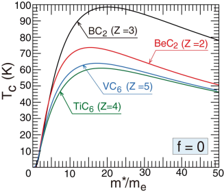
Figure 4: Prediction of $T_{c}$ as a function of $m^{*}$ for various GICs in pursuit of optimum $T_{c}$. We assume the fractional factor $f=0$.

We have explored the optimum $T_{c}$ in the whole family of GICs by widely changing various parameters involved in the microscopic Hamiltonian of the standard model. Examples of the calculated results of $T_{c}$ are shown in Fig. 4, in which $f$ is fixed to zero, the optimum condition to raise $T_{c}$, and $d$ is tentatively taken as 4.0Å. From this exploration, we find that the most important parameter to enhance $T_{c}$ is $m^{*}$. In particular, we need $m^{*}$ larger than at least $2m_{e}$ to obtain $T_{c}$ over 10K, irrespective of any choice of other parameters, and $T_{c}$ is optimized for $m^{*}$ in the range $(10-20)m_{e}$. The optimized $T_{c}$ depends rather strongly on the parameters to control the polar-coupling strength such as $Z$ and the atomic mass $A$; if we choose a trivalent light atom such as boron to make $\omega_{t}(0)$ large, the optimum $T_{c}$ is about 100K, but the problem about the light atoms is that $m^{*}$ will never become heavy due to the absence of either d or f electrons. Therefore we do not expect that $T_{c}$ would become much larger than 10K, even if BeC₂ or BC₂ were synthesized. From this perspective, it will be much better to intercalate Ti or V, rather than Be or B. Taking all these points into account, we suggest synthesizing three-element GICs providing a heavy 3D electron system by the introduction of heavy atoms into a light-atom polar-crystal environment.

IV Strong-Coupling Approach with Application to Fullerides

IV.1 Coherence Length

In the BCS theory for superconductivity which is applicable to superconductors in the weak-coupling region, $T_{c}$ is directly related to the coherence length $\xi_{0}$ which characterizes the spatial extent of the wave function representing the bound state of a Cooper pair at zero temperature. More concretely, the relation between them is expressed as $T_{c}/E_{F}=2e^{\gamma}/\pi^{2}(p_{F}\xi_{0})^{-1}\approx 0.361/p_{F}\xi_{0}$ with $\gamma\,(=0.57721\cdots)$ the Euler-Mascheroni constant and $p_{F}$ the Fermi wave number. Because $p_{F}^{-1}$ is in proportion to the lattice constant $a_{0}$, the relation is rewritten into the form as

$${T_{c}\over E_{F}}\ \approx\ 0.0735\,{a_{0}\over\xi_{0}}$$ (16)

for a monovalent metal in the fcc-lattice structure. (For other valence and/or crystal structure, the coefficient of 0.0735 changes, but it always remains in the same order of magnitude.) For usual elemental superconductors, $T_{c}/E_{F}$ is of the order of $10^{-4}$ and thus $\xi_{0}$ is about a thousand times larger than $a_{0}$, validating the approach in momentum space. On the other hand, the relation in Eq. (16) implies that high $T_{c}$ is inevitably associated with short $\xi_{0}$. In fact, $\xi_{0}$ is observed as only a few nm or less, i.e., of the same order of $a_{0}$ in many of the recently synthesized high-$T_{c}$ superconductors Text such as the cuprates, the alkali-doped C₆₀, and MgB₂.

A similar message can be obtained through the so-called Uemura plot Uemura91a ; Uemura91b ; Takada92 , according to which there is a universal relation of $T_{c}/E_{F}\approx 0.04$ for a wide variety of strong-coupling superconductors. If this relation is put into Eq. (16), we obtain $\xi_{0}\approx 2\,a_{0}$. Furthermore, if we think of the Bose-Einstein condensation (BEC) for an assembly of very tightly-bound pairs of electrons, the condensation temperature (which amounts to $T_{c}$ in such a system) is given by $T_{c}/E_{F}=(2/9\pi\,\zeta(3/2)^{2})^{1/3}\approx 0.218$, where $\zeta(3/2)\,(=2.6124\cdots)$ is the Riemann’s zeta function $\zeta(x)$ at $x=3/2$. This value of $T_{c}/E_{F}$ (which must be the optimum value for fermionic superconductors) suggests $\xi_{0}\approx 0.3\,a_{0}$. Thus, in treating superconductivity in the strong-coupling region, we need to consider a situation of extremely short $\xi_{0}$, validating the approach in real space, which is totally different from that of very long $\xi_{0}$ in the weak-coupling superconductors.

IV.2 Pairing Interaction in the Strong-Coupling Region

In view of the above-mentioned difference in $\xi_{0}$, we shall exploit the shortness of $\xi_{0}$ in reformulating the problem of making a quantitative calculation of $T_{c}$ for strong-coupling superconductors in the Green’s-function approach Takada07 . Let us start with this reformulation by considering the dynamical correlation function for singlet pairing of two electrons in the normal state $Q_{sc}^{R}({\bm{q}},\omega)$, which is defined as

$$Q_{sc}^{R}({\bm{q}},\omega)=-i\int_{0}^{\infty}dt\,e^{i\omega t-\eta t}\langle[e^{iHt}\Phi_{\bm{q}}e^{-iHt},\Phi_{\bm{q}}^{+}]\rangle,$$ (17)

where $H$ is the Hamiltonian for a homogeneous electron system and $\Phi_{\bm{q}}$ is the electron-pair annihilation operator, defined by $\Phi_{\bm{q}}\,\equiv\sum_{\bm{p}}c_{{\bm{p}}+{\bm{q}}\uparrow}c_{-{\bm{p}}\downarrow}$. In terms of the retarded pairing correlation function $Q_{sc}^{R}({\bm{q}},\omega)$, we can define $T_{c}$ as the temperature at which $Q_{sc}^{R}({\bm{q}},\omega)$ diverges at ${\bm{q}}={\bm{0}}$ in the static limit ($\omega\to 0$) with the decrease of $T$.

As shown schematically in Fig. 5(a), $Q_{sc}$ is conventionally divided into a sum of terms classified by the number of $\tilde{J}$s, where $\tilde{J}$, which has already appeared in Eq. (4), is the irreducible electron-electron effective interaction including all vertex corrections. Using $\Pi_{sc}({\bm{q}},\omega)$ the pairing polarization function composed of two full electron Green’s functions including all self-energy corrections, we can express the infinite sum in Fig. 5(a) in a quite symbolical way as

$$Q_{sc}=-{\Pi_{sc}\over 1+{\tilde{J}}\,\Pi_{sc}}.$$ (18)

Then, the divergence in $Q_{sc}^{R}({\bm{0}},\omega\to 0)$ occurs at the zero of the denominator in Eq. (18), which provides exactly the same $T_{c}$ as that obtained through the solution of Eq. (4).

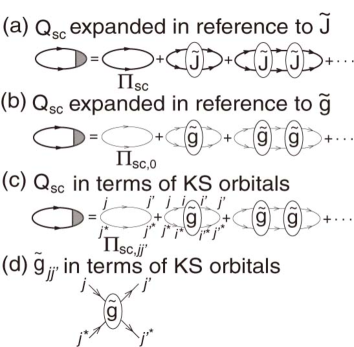
Figure 5: Pair correlation function $Q_{sc}$ described in terms of using either (a) the pairing polarization function $\Pi_{sc}$ and the irreducible electron-electron effective interaction $\tilde{J}$ or (b) the noninteracting pairing polarization function $\Pi_{sc,0}$ and the effective interaction ${\tilde{g}}$. By the extension of the idea of expanding $Q_{sc}$ with use of $\Pi_{sc,0}$, we show a scheme to express it in terms of Kohn-Sham orbitals in (c), together with the schematic representation of ${\tilde{g}}_{jj^{\prime}}$ in (d).

Now, instead of using $\Pi_{sc}$, we shall consider an alternative expansion with use of $\Pi_{sc,0}$ the pairing polarization function composed of two bare electron Green’s functions. As shown schematically in Fig. 5(b), if we introduce the pairing interaction ${\tilde{g}}$ by the definition of

$${\tilde{g}}\equiv{\tilde{J}}+{1\over\Pi_{sc}}-{1\over\Pi_{sc,0}},$$ (19)

we can rewrite $Q_{sc}$ in Eq. (18) into another exact form as

$$Q_{sc}=-{\Pi_{sc,0}\over 1+{\tilde{g}}\,\Pi_{sc,0}}.$$ (20)

Since we can always calculate $\Pi_{sc,0}$ easily, the problem of estimating $T_{c}$ is reduced to the evaluation of ${\tilde{g}}$ in the limit of $\omega\to 0$ at ${\bm{q}}={\bm{0}}$. Note that ${\tilde{g}}$ does not depend strongly on either ${\bm{q}}$ or $\omega$, in sharp contrast with $\Pi_{sc,0}^{R}({\bm{q}},\omega)$. In the BCS theory, for example, ${\tilde{g}}$ is taken as a constant which represents a weakly attractive and spatially local interaction working only in the vicinity of the Fermi level, given that the phonon energy $\omega_{0}$ is much smaller than $E_{F}$. Then the zero of the denominator in Eq. (20) at ${\bm{q}}={\bm{0}}$ and $\omega\to 0$ provides the well-known BCS formula for $T_{c}$. Note also that the problem of finding the zero of $1+{\tilde{g}}\,\Pi_{sc,0}^{R}({\bm{0}},\omega\to 0)$ is just the same as that of solving the gap equation in Eq. (6) with replacing $V({\bm{p}}\!-\!{\bm{p}^{\prime}},i\omega_{p}\!-\!i\omega_{p^{\prime}})$ by ${\tilde{g}}$.

In the case of short $\xi_{0}$, we may assume that the essential physics of electron pairing can be captured even if we treat only a small-cluster system, as long as the system size is large enough in comparison with $\xi_{0}$. Under this assumption, we can take the following procedure for determining ${\tilde{g}}$: First, by representing the values for $\Pi_{sc,0}$ and ${\tilde{g}}$ in an $N$-site system as $\Pi_{sc,0}^{(N)}$ and ${\tilde{g}}_{N}$, respectively, we may write the pairing correlation function for the $N$-site system $Q_{sc}^{(N)}$ as

$$Q_{sc}^{(N)}=-\,{\Pi_{sc,0}^{(N)}\over 1+{\tilde{g}}_{N}\Pi_{sc,0}^{(N)}},$$ (21)

in accordance with Eq. (20). In general, the exact bulk value ${\tilde{g}}$ will be obtained by taking the large-$N$ limit of ${\tilde{g}}_{N}$, but expecting that ${\tilde{g}}_{N_{0}}$ with a small positive integer $N_{0}$ (for example, $N_{0}\approx 2$) is already close to ${\tilde{g}}$, we may estimate ${\tilde{g}}$ by the relation of

$${\tilde{g}}=-{1\over Q_{sc,0}^{(N_{0})}}-{1\over\Pi_{sc,0}^{(N_{0})}},$$ (22)

with $Q_{sc}^{(N_{0})}$ evaluated rigorously, for example, by exact diagonalization. Of course, we can determine a better value of ${\tilde{g}}$ by checking the saturation behavior of $\{{\tilde{g}}_{N_{0}}\}$ with the increase of $N_{0}$.

IV.3 Interpolation Formula for the Pairing-Interaction Functional

Based on the knowledge so far obtained, let us speculate an appropriate functional form for the pairing interaction ${\cal K}_{jj^{\prime}}$ in SCDFT. It would be natural to expand the electron field operator in terms of the Kohn-Sham orbitals $\{|j\rangle\}$ in an inhomogeneous electron system, so that we can define the electron-pair operator $\Phi_{j}$ as $\Phi_{j}\,\equiv c_{j}c_{{j}^{*}}$ with $|{j}^{*}\rangle$ the time-reversed orbital of $|{j}\rangle$. Then, we can introduce the pairing polarization function in terms of $\Phi_{j}$ and $\Phi_{j^{\prime}}^{+}$. In particular, we can calculate this quantity in the noninteractiong system $\Pi_{sc,jj^{\prime}}$ in analogy with $\Pi_{sc,0}$, as schematically introduced in Fig. 5(c). At the same time, we can define a quantity ${\tilde{g}}_{jj^{\prime}}$ as schematically shown in Fig. 5(d).

In the strong-coupling region, we do not expect that this ${\tilde{g}}_{jj^{\prime}}$ exhibits strong dependence on $i\Omega$, because the Fermi energy, the scale for the electron kinetic energy, must be much smaller than the energy scale representing electron-electron interactions. In addition, ${\tilde{g}}_{jj^{\prime}}$ does not depend strongly on orbital variables, either, because the pairing interaction should be short-ranged in real space in line with the shortness of $\xi_{0}$. Thus we may regard ${\tilde{g}}_{jj^{\prime}}$ as a constant. Then, if we take ${\cal K}_{jj^{\prime}}$ in Eq. (1) as ${\tilde{g}}_{jj^{\prime}}$, we can easily see that both Eq. (1) and the zero of $1+{\tilde{g}}_{jj^{\prime}}\,\Pi_{sc,jj^{\prime}}^{R}$ provide the same $T_{c}$.

In a more general situation of the intermediate-coupling region, however, ${\tilde{g}}_{jj^{\prime}}$ will depend on both $i\Omega$ and orbital variables. In order to treat such a situation and also by paying attention to the weak-coupling situation examined in the previous section, we propose the functional form for ${\cal K}_{jj^{\prime}}$ in exactly the same form as that in Eq. (11) with replacing $V_{jj^{\prime}}(i\Omega)$ by ${\tilde{g}}_{jj^{\prime}}(i\Omega)$. Note that this functional form of ${\cal K}_{jj^{\prime}}$ is reduced to ${\tilde{g}}_{jj^{\prime}}(0)$, if ${\tilde{g}}_{jj^{\prime}}(i\Omega)$ does not depend on $\Omega$, assuring us that the framework in SCDFT with this choice of ${\cal K}_{jj^{\prime}}$ provides the same $T_{c}$ as that in the usual Green’s-function approach in the strong-coupling region. This means that we can successfully take care of both self-energy and vertex corrections beyond the G₀W₀ approximation by upgrading $V_{jj^{\prime}}(i\Omega)$ to ${\tilde{g}}_{jj^{\prime}}(i\Omega)$ in Eq. (11).

IV.4 Alkali-Doped Fullerides

IV.4.1 Aims of This Subsection

The fulleride is a molecular crystal with narrow threefold conduction bands (with the band width $W\approx 0.5$eV) derived from the $t_{1u}$ electronic levels of each C₆₀ molecule. With the doping of three alkali atoms per one C₆₀ molecule, we obtain the half-filled situation in which superconductivity occurs with $T_{c}$ in the range $18-38$K Hebard91 ; Takabayashi09 and the short coherence length $\xi_{0}$ of only a few molecular units. As for the mechanism of superconductivity in the alkali-doped fullerides, phonons are widely believed to play an important role. This belief is based upon a crude estimate of $T_{c}$ in the conventional Eliashberg theory. In fact, analysis of various experiments with use of this theory has shown that many aspects of superconductivity in these fullerides are consistent with a picture of $s$-wave BCS superconductors with the Cooper pairs driven by the coupling to the intramolecular high-frequency phonons in $H_{g}$ symmetry (with the phonon energy $\omega_{0}\approx 0.2$eV and the nondimensional electron-phonon coupling constant $\lambda\approx 0.6$ for Rb₃C₆₀) Gunnarsson97 ; Ramirez ; Gelfand .

The above picture, however, seems to be too much simplified and we may raise several fundamental questions. From a theoretical point of view, one of the serious problems is ill foundation to adopt the Eliashberg theory in the fullerides due to the importance of vertex corrections Takada93b ; vertex . From an experimental side, the following four experimental facts have been observed which we cannot easily understand with use of the Eliashberg theory: (i) The relation between $T_{c}$ and the lattice constant $a_{0}$ changes remarkably when the crystal structure changes from the face centered cubic (fcc) to simple cubic (sc) lattice by the introduction of Na, a smaller ion compared to K, Rb, or Cs, as a dopant ion Tanigaki . (ii) The antiferromagnetic (AF) insulating behavior has been reported in ammoniated K₃C₆₀, which is peculiar in the sense that $s$-wave BCS superconductivity exists in the vicinity of an AF phase Iwasa . A similar problem is also seen in the body-centered cubic A15-structured Cs₃C₆₀ Takabayashi09 . (iii) The anomalous ¹³C isotope effect on $T_{c}$ for 50% ¹³C substitution has been observed, reflecting the difference between the molecular and atomic mixture of ¹²C and ¹³C atoms Lieber . (iv) With the deviation of electron number per site $n$ from half-filling, $T_{c}$ decreases rapidly in both sides of the deviation Yildirim .

Although the experiment (i) may be reproduced in the Eliashberg theory with some judicious choice of parameters, the rest (ii)-(iv) cannot be explained even qualitatively in the theory. In addition, the behavior of $T_{c}$ as a function of $n$ observed in the experiment (iv) cannot be predicted either by those theories proposed so far to account for the copper-oxide high-$T_{c}$ superconductivity based on some strong-correlation models, though such models may be favorable for the explanation of the experiment (ii).

A successful theory for the fullerene superconductors should not only reproduce these experiments in a coherent fashion but also clarify the reason why the effect of vertex corrections, even if it is large, does not manifest itself in many superconducting properties. In quest of such a theory from a somewhat general viewpoint, the present author made intensive studies of the Hubbard-Holstein (HH) model and its extension in the past and successfully explained all the issues (i)-(iv) raised above Takada98 ; Takada1 ; Takada2 ; Takada3 ; Hotta1 ; Hotta . In the rest of this subsection, we shall focus on the first three issues in order to show how nicely the HH model applies to the fullerides, as far as $T_{c}$ is concerned. Then we shall explore a possibility to enhance $T_{c}$ in this class of superconductors by changing the parameters involved in the model.

IV.4.2 The Hubbard-Holstein Model

In a molecular crystal, it is a very good approximation to regard each molecular unit as a “site” in a lattice. We shall adopt this approximation and describe the electron-phonon system in the alkali-doped fullerides by a model Hamiltonian $H$ in site representation in which each site corresponds to each C₆₀ molecular unit. Since the conduction band width is narrow, the intermolecular hopping integral $t$ must be small, indicating that only the nearest-neighbor hopping is relevant in modelling the kinetic energy of the system. Then, it would be appropriate to decompose $H$ into the nearest-neighbor electron-transfer term $H_{t}$ and the sum of site terms $\sum_{i}H_{i}$ including both the electron-electron and the electron-local phonon interactions. In order to faithfully represent the threefold degenerate $t_{1u}$-conduction bands coupled with eight $H_{g}$ intramolecular Jahn-Teller (JT) phonons, we would need to include the $t_{1u}\otimes H_{g}$ JT structure in $H_{i}$, as has often been the case Varma ; Manini94a ; Manini94b ; Gunnarsson03 . In making a detailed study on the stability of the AF insulating phase, it is known that this feature of band multiplicity plays a rather crucial role Gunnarsson00 , but in treating superconductivity itself, the band multiplicity is not considered to be of primary importance Cappelluti05 . Therefore we shall take a simplest possible model, namely, the one-band HH model to discuss superconductivity from a more general viewpoint that will be applicable to the whole family of fullerene superconductors including not only electron-doped but also hole-doped materials with different JT structures.

The concrete form for $H$ in the HH model is given by

$$H=-t\sum_{\langle i,i^{\prime}\rangle\,\sigma}(c_{i\sigma}^{\dagger}c_{i^{\prime}\sigma}+{\rm h.c.})+\sum_{i}H_{i},$$ (23)

with the site term $H_{i}$, written as

$$H_{i} =-\mu\sum_{\sigma}n_{i\sigma}+U\,n_{i\uparrow}n_{i\downarrow}$$

$$+\sqrt{\alpha}\omega_{0}\sum_{\sigma}n_{i\sigma}(a_{i}+a_{i}^{\dagger})+\omega_{0}\,a_{i}^{\dagger}a_{i},$$ (24)

where $\langle i,i^{\prime}\rangle$ represents the nearest-neighbor-site pair, $c_{i\sigma}$ the operator to annihilate a spin-$\sigma$ electron at site $i$, $\mu$ the chemical potential, $n_{i\sigma}\equiv c_{i\sigma}^{\dagger}c_{i\sigma}$, $U$ the on-site (or intramolecular) Coulomb repulsion, $\alpha$ the nondimensional electron-phonon coupling constant which is related to the conventional electron-phonon coupling constant $\lambda$ through $\lambda=\alpha\omega_{0}/tz$ with $\omega_{0}$ the optical-phonon energy and $z$ the coordination number, and $a_{i}$ the operator to annihilate an optical phonon at site $i$.

The characteristic features of the fullerenes can be well captured by an appropriate choice of the parameters involved in this Hamiltonian. In fact, the narrowness of the conduction band can be described by the smallness of $t$ of the order of 0.1eV. The difference in the crystal structure as well as the effect of band multiplicity can be well accounted for by a suitable choice of $z$. The high-frequency intramolecular optical phonons coupled strongly to electrons can be treated by considering the local phonons with the energy $\omega_{0}\,(\approx 0.2$eV) at each site. The short-range Coulomb potential must be relevant in the fullerenes due to the proximity to the AF state and it can be included by the introduction of $U$. Note that this $U$ is not the direct Coulomb repulsion between electrons on a carbon atom $U_{\rm atom}$ which is of the order of 5-10eV. Rather it is the sum of $U_{\rm atom}$ and the attraction $-U_{\rm pol}$ due to the electronic polarization effect of 60 $\pi$-electrons in the C₆₀ molecule Chakravarty . Because of a strong cancellation between $U_{\rm atom}$ and $-U_{\rm pol}$, $U$ is expected to be of the order of 0.1eV, which is about the same magnitude as that for the phonon-mediated attraction, $-U_{ph}\equiv-2\alpha\omega_{0}$.

Intensive studies on the ground state in this system by exact diagonalization of small-size clusters have revealed that the half-filled HH model exhibits interesting competition among charge-density-wave (CDW), spin-density-wave (SDW), and superconducting states Takada2 ; Hotta1 . We may summarize the results in the following way: (a) If $U-U_{ph}$ is at least smaller than $-t$, the CDW state composed of an array of immobile bipolarons is stabilized. (b) If $U-U_{ph}$ is larger than $t$, there appears the SDW state which is nothing but the AF state in this case. (c) Superconductivity appears only in the CDW-SDW transition region where $|U-U_{ph}|$ is less than $t$. In this offset situation of $U\approx U_{ph}$, the state may be regarded as an assembly of nearly free polarons and the main effect of the strong electron-phonon vertex corrections is found to form a polaron from a bare electron. This implies that the Eliashberg theory or even the BCS theory is expected to be accurate enough to describe superconductivity in this system, if it is applied on the basis of the polaron picture Takada2 ; Hotta1 ; Alexandrov1 . In any case, the intrisic competition of superconductivity with the AF state in the half-filled HH model resolves the issue (ii) raised previously.

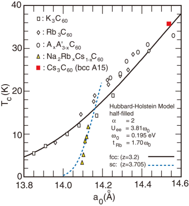
Figure 6: $T_{c}$ as a function of the lattice constant $a_{0}$ in the alkali-doped fullerides and its dependence on the crystal structure. The solid and the broken curves represent our theoretical results, while the experimental results are given by square, triangle, diamond, and circle marks.

In order to address the issue (i), we have applied our framework to calculate $T_{c}$ to the HH model by estimating ${\tilde{g}}$ with use of a cluster as small as two molecules (i.e., $N_{0}=2$). We have evaluated the variation of $t$ with the change of the lattice constant $a_{0}$ by fitting the change in the band width obtained by the band-structure calculation for each lattice structure Satpathy ; Saito . More specifically, $t$ is determined by

$$t=t_{\rm Rb}\,{d\over d_{\rm Rb}}\,\exp\left(-{d-d_{\rm Rb}\over\Delta}\right),$$ (25)

with $d=a_{0}/\sqrt{2}-6.95$Å , $\Delta=0.55$Å , and the corresponding parameters, $t_{\rm Rb}$ and $d_{\rm Rb}$, for Rb₃C₆₀. By choosing $t_{\rm Rb}=1.70\omega_{0}$ suitable for Rb₃C₆₀ and the common parameters such as $U=3.81\omega_{0}$, $\alpha=2$, and $\omega_{0}=0.195$eV with reference to band-structure calculations and relevant experiments, we obtain the results for $T_{c}$ as a function of $a_{0}$, which agrees remarkably well with experiment as clearly demonstrated in Fig. 6 Note that in our calculation, the difference in $T_{c}$ between fcc and sc structures arises mainly from that in the “effective” lattice coordination number $z$ Gelfand . This indicates that $z$ is a key to the resolution of the issue (i). Note also that the recent experimental result for Cs₃C₆₀ under pressure is also on our theoretical curve, if we estimate an appropriate value of $a_{0}$ so as to reproduce the same volume per one C₆₀ molecule for this bcc A15 structure.

The competing feature between $U_{ph}$ and $U$ is also identified to be a key to the resolution of the issue (iii) Takada3 . The observed anomalous isotope effect cannot be explained by either the phonon or the electronic polarization mechanism alone. It can be reproduced, if both these mechanisms are included simultaneously. Namely, we need to consider the change in both $\omega_{0}$ and $U$ induced by the isotope substitution. The sensitivity of $T_{c}$ to the local change in the Coulomb potential $U$ is due to the very short-range nature of $\xi_{0}$ of this superconductivity.

IV.4.3 Prospect for Room-Temperature Superconductors

Encouraged by the success in reproducing $T_{c}$ for the alkali-doped fullerene superconductors by the application of our theoretical framework to the HH model at half-filling in the nearly offset situation of $U\approx U_{ph}$, we have attempted to explore the optimum value of $T_{c}$ with the increase of the electron-phonon coupling constant $\alpha$, whereby $U$ is also increased to keep the offset situation. Examples of the calculated results of $T_{c}$ are plotted in Fig. 7 As is seen, $T_{c}$ goes beyond 100K for $\alpha=3$ and it reaches room temperature for $\alpha=4$.

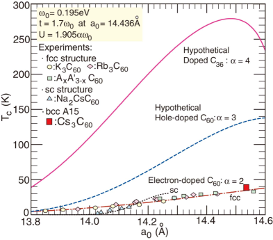
Figure 7: $T_{c}$ as a function of the lattice constant $a_{0}$. For electron-doped C₆₀ with $\alpha=2$, the theoretical curves are drawn, together with the experimental results. We also give the results for both $\alpha=3$ and $4$ corresponding to (hypothetical) hole-doped C₆₀ and doped C₃₆.

By the band-structure calculation Mazin3 , it is known that $\alpha$ is about three for the hole-doped C₆₀ in which hole carriers will be introduced into the $h_{u}$-valence bands. On the other hand, in the crystal composed of C₃₆, $\alpha$ will be about four Cohen , if the C₃₆ solid is successfully doped to have an enough number of mobile carriers in the system, although it seems to be a very difficult task Zettl .

V Conclusion and Discussion

In this chapter, we have proposed a new functional form for the pairing interaction ${\cal K}_{jj^{\prime}}$, a key quantity in the gap equation, Eq. (1), to determine $T_{c}$ in the density functional theory for superconductors. The functional form is given in Eq. (11) with the effective electron-electron interaction $V_{jj^{\prime}}(i\Omega)$ replaced by ${\tilde{g}}_{jj^{\prime}}(i\Omega)$ defined schematically in Fig. 5(d). We have assessed the usefulness of this functional form by its applications to both the weak-coupling superconductors like the alkali- and alkaline-earth-intercalated graphites and the strong-coupling superconductors like the alkali-doped fullerides. We have also explored a possibility to enhance $T_{c}$ up to room temperature.

The proposed functional form has just opened a challenging frontier of the research on high-$T_{c}$ superconductivity. Although we need to improve on the functional form itself by utilizing the information obtained by its application to a much wider range of materials, we can think of several ways to make use of this new theoretical tool. For example, we can make a quantitative assessment of the effectiveness of each superconducting mechanism, either phononic or electronic, so far proposed by investigating how much $T_{c}$ is actually enhanced with the introduction of the mechanism. The knowledge accumulated by such investigations will pave the way to reach a room-temperature superconductor.

VI Acknowledgments

This work is supported by a Grant-in-Aid for Scientific Research (C) (No. 21540353) from MEXT, Japan.

References

- (1) W. L. McMillan, Phys. Rev. 167, 331 (1968).
- (2) P. B. Allen and R. C. Dynes, Phys. Rev. B 12, 905 (1975).
- (3) P. B. Allen and B. Mitrović, in Solid State Physics, edited by H. Ehrenreich, F. Seitz, and D. Turnbull, Vol. 37, p. 1 (Academic, New York, 1982).
- (4) J.P. Carbotte, Rev. Mod. Phys. 62, 1027 1990.
- (5) G. M. Eliashberg, Sov. Phys.-JETP 11, 696 (1960).
- (6) P. Morel and P. W. Anderson, Phys. Rev. 125, 1263 (1962).
- (7) K.-P. Bohnen, R. Heid, and B. Renker, Phys. Rev. Lett. 86, 5771 (2001).
- (8) Y. Kong, O. V. Dolgov, O. Jepsen, and O. K. Andersen, Phys. Rev. B 64, 020501(R) (2001).
- (9) H. J. Choi, D. Roundy, H. Sun, M. L. Cohen, and S. G. Louie, Nature 418, 758 (2002).
- (10) H. J. Choi, D. Roundy, H. Sun, M. L. Cohen, and S. G. Louie, Phys. Rev. B 66, 020513(R) (2002).
- (11) I. I. Mazin, Phys. Rev. Lett. 95, 227001 (2005).
- (12) M. Calandra and F. Mauri, Phys. Rev. Lett. 95, 237002 (2005).
- (13) Y. Takada, J. Phys. Soc. Jpn. 45, 786 (1978).
- (14) Y. Takada, Phys. Rev. B 47, 5202 (1993).
- (15) A. F. Hebard, M. J. Rosseinsky, R. C. Haddon, D. W. Murphy, S. H. Glarum, T. T. M. Palstra, A. P. Ramirez, and A. R. Kortan, Nature 350, 600 (1991).
- (16) Y. Takabayashi, A. Y. Ganin, P. Jeglič, D. Arčon, T. Takano, Y. Iwasa, Y. Ohishi, M. Takata, N. Takeshita, K. Prassides, and M. J. Rosseinsky, Science 323, 1585 (2009).
- (17) O. Gunnarsson, Rev. Mod. Phys. 69, 575 (1997).
- (18) Y. Takada and T. Hotta, Int. J. Mod. Phys. B 12, 3042 (1998).
- (19) Y. Takada, J. Phys. Chem. Solids 54, 1779 (1993).
- (20) Y. Takada, Phys. Rev. B 52, 12708 (1995).
- (21) Y. Takada, Phys. Rev. Lett. 87, 226402 (2001).
- (22) L. N. Oliveira, E. K. U. Gross, and W. Kohn, Phys. Rev. Lett. 60, 2430 (1988).
- (23) S. Kurth, M. Marques, M. Lüders, and E. K. U. Gross, Phys. Rev. Lett. 83, 2628 (1999).
- (24) Y. Takada, J. Phys. Soc. Jpn. 78, 013703 (2009).
- (25) Y. Takada, J. Supercond. Nov. Magn. 22, 89 (2009).
- (26) Y. Takada, Int. J. Mod. Phys. B 21, 3138 (2007).
- (27) P. Hohenberg and W. Kohn, Phys. Rev. 136, 864 (1964).
- (28) W. Kohn and L. J. Sham, Phys. Rev. 140, A1133 (1965).
- (29) P. G. de Gennes, Superconductivity of Metals and Alloys, (Benjamin, New York, 1966).
- (30) Throughout this article, we use the units in which .
- (31) J. P. Perdew and M. Levy, Phys. Rev. Lett. 51, 1884 (1983).
- (32) L. J. Sham and M. Schlüter, Phys. Rev. Lett. 51, 1888 (1983)
- (33) L. J. Sham and M. Schlüter, Phys. Rev. B 32, 3883 (1985).
- (34) M. Lüders, M. A. L. Marques, N. N. Lathiotakis, A. Floris, G. Profeta, L. Fast, A. Continenza, S. Massidda, and E. K. U. Gross, Phys. Rev. B 72, 024545 (2005).
- (35) A. Sanna, G. Profeta, A. Floris, A. Marini, E. K. U. Gross, and S. Massidda, Phys. Rev. B 75, 020511(R) (2007).
- (36) M. A. L. Marques, M. Lüders, N. N. Lathiotakis, G. Profeta, A. Floris, L. Fast, A. Continenza, E. K. U. Gross, and S. Massidda, Phys. Rev. B 72, 024546 (2005).
- (37) A. Floris, G. Profeta, N. N. Lathiotakis, M. Lüders, M. A. L. Marques, C. Franchini, E. K. U. Gross, A. Continenza, and S. Massidda, Phys. Rev. Lett. 94, 037004 (2005).
- (38) G. Profeta, C. Franchini, N. N. Lathiotakis, A. Floris, A. Sanna, M. A. L. Marques, M. Lüders, S. Massidda, E. K. U. Gross, and A. Continenza, Phys. Rev. Lett. 96, 047003 (2006).
- (39) A. Sanna, C. Franchini, A. Floris, G. Profeta, N. N. Lathiotakis, M. Lüders, M. A. L. Marques, E. K. U. Gross, A. Continenza, and S. Massidda, Phys. Rev. B 73, 144512 (2006).
- (40) A. Floris, A. Sanna, S. Massidda, and E. K. U. Gross, Phys. Rev. B 75, 054508 (2007).
- (41) J. P. Perdew, K. Burke, and M. Ernzerhof, Phys. Rev. Lett. 77, 3865 (1996); ibid. 78, 1396 (1997) (E).
- (42) M. L. Cohen, Phys. Rev. 134 A511 (1964).
- (43) M. L. Cohen, in “Superconductivity”, ed.R. D. Parks (Marcel Dekker, New York, 1969) Vol. 1, Chap. 12.
- (44) Y. Takada, J. Phys. Soc. Jpn. 49, 1267 (1980).
- (45) D. A. Kirzhnits, E. G. Maksimov, and D. I. Khomskii, J. Low Temp. Phys. 10, 79 (1973).
- (46) C. S. Koonce, M. L. Cohen, J. F. Schooley, W. R. Hosler, and E. R. Pfeiffer, Phys. Rev. 163, 380 (1967).
- (47) X. Lin, Z. Zhu, B. Fauqué, and K. Behnia, Phys. Rev. X 3, 021002 (2013).
- (48) J. E. Fischer and T. E. Thompson, Phys. Today 31, Issue 7, 36 i1978).
- (49) H. Kamimura, Phys. Today 40, Issue 12, 64 (1987).
- (50) H. Zabel and S. A. Solin (Eds.), Graphite Intercalation Compounds II, Springer-Verlag, 1992.
- (51) M. S. Dresselhaus and G. Dresselhaus, Adv. Phys. 51, 1 (2002).
- (52) N. B. Hannay, T. H. Geballe, B. T. Matthias, K. Andres, P. Schmidt, and D. MacNair, Phys. Rev. Lett. 14, 225 (1965).
- (53) Y. Koike, H. Suematsu, K. Higuchi, and S. Tanuma, Solid State Commun. 27, 623 (1978).
- (54) M. Kobayashi and I. Tsujikawa, J. Phys. Soc. Jpn. 46, 1945 (1979).
- (55) Y. Koike, H. Suematsu, K. Higuchi, and S. Tanuma, Physica B 99, 503 (1980).
- (56) M. G. Alexander, D. P. Goshorn, D. Guerard, P. Lagrange, M. El Makrini, and D. G. Onn, Synth. Met. 2, 203 (1980).
- (57) Y. Iye and S. Tanuma, Phys. Rev. B 25, 4583 (1982).
- (58) I. T. Belash, O.V. Zharikov, and A.V. Pal’nichenko, Synth. Met. 34, 455 (1989).
- (59) M. S. Dresselhaus, A. Chaiken, and G. Dresselhaus, Synth. Met. 34, 449 (1989).
- (60) I. T. Belash, A. D. Bronnikov, O.V. Zharikov, and A.V. Pal’nichenko, Synth. Met. 36, 283 (1990).
- (61) I. T. Belash, A. D. Bronnikov, O.V. Zharikov, and A.V. Pal’nichenko, Solid State Commun. 69, 921 (1989).
- (62) T. E. Weller, M. Ellerby, A. S. Saxena, R. P. Smith, and N. T. Skipper, Nature Phys. 1, 39 (2005).
- (63) N. Emery, C. Heérold, M. d’Astuto, V. Garcia, C. Bellin, J. F. Marêché, P. Lagrange, and G. Loupias, Phys. Rev. Lett. 95, 087003 (2005).
- (64) A. Gauzzi, S. Takashima, N. Takeshita, C. Terakura, H. Takagi, N. Emery, C. Hérold, P. Lagrange, and G. Loupias, Phys. Rev. Lett. 98, 067002 (2007).
- (65) J. S. Kim, L. Boeri, J. R. O’Brien, F. S. Razavi, and R. K. Kremer, Phys. Rev. Lett. 99, 027001 (2007).
- (66) J. S. Kim, R. K. Kremer, L. Boeri, and F. S. Razavi, Phys. Rev. Lett. 96, 217002 (2006).
- (67) C. Kurter, L. Ozyuzer, D. Mazur, J. F. Zasadzinski, D. Rosenmann, H. Claus, D. G. Hinks, and K. E. Gray, Phys. Rev. B 76, 220502 (2007).
- (68) G. Csanyi, P. B. Littlewood, A. H. Nevidomskyy, C. J. Pickard, and B. D. Simons, Nature Phys. 1, 42 (2005).
- (69) D. G. Hinks, D. Rosenmann, H. Claus, M. S. Bailey, and J. D. Jorgensen, Phys. Rev. B 75, 014509 (2007).
- (70) M. Posternak, A. Baldereschi, A. J. Freeman, and E. Wimmer, Phys. Rev. Lett. 52, 863 (1984).
- (71) N. A. W. Holzwarth, S. G. Louie, and S. Rabii, Phys. Rev. B 30, 2219 (1984).
- (72) A. Koma, K. Miki, H. Suematsu, T. Ohno, and H. Kamimura, Phys. Rev. B 34, 2434 (1986).
- (73) T. Ohno, K. Nakao, and H. Kamimura, J. Phys. Soc. Jpn. 47, 1125 (1979).
- (74) G. Wang, W. R. Datars, and P. K. Ummat, Phys. Rev. B 44, 8294 (1991).
- (75) Y. Takada, J. Phys. Soc. Jpn. 51, 63 (1982).
- (76) U. Mizutani, T. Kondow, and T. B. Massalski, Phys. Rev. B 17, 3165 (1978).
- (77) See, for example, C. P. Poole, Jr., Handbook of Superconductivity, (Academic, San Diego, 2000).
- (78) Y. J. Uemura, L. P. Le, G. M. Luke, B. J. Sternlieb, W. D. Wu, J. H. Brewer, T. M. Riseman, C. L. Seaman, M. B. Maple, M. Ishikawa, D. G. Hinks, J. D. Jorgensen, G. Saito, and H. Yamochi, Phys. Rev. Lett. 66, 2665 (1991).
- (79) Y. J. Uemura, A. Keren, L. P. Le, G. M. Luke, B. J. Sternlieb, W. D. Wu, J. H. Brewer, R. L. Whetten, S. M. Huang, Sophia Lin, R. B. Kaner, F. Diederich, S. Donovan, G. Grüner, and K. Holczer, Nature 352, 605 (1991).
- (80) Y. Takada, J. Phys. Soc. Jpn. 61, 3849 (1992).
- (81) A. P. Ramirez, Superconductivity Review 1, 1 (1994).
- (82) M. P. Gelfand, Superconductivity Review 1, 103 (1994).
- (83) L. Pietronero, Europhys. Lett. 17, 365 (1992).
- (84) K. Tanigaki, I. Hirosawa, T. W. Ebbesen, J. Mizuki, and J.-S. Tsai, J. Phys. Chem. Solids 54, 1645 (1993).
- (85) Y. Iwasa, H. Shimoda, T. T. M. Palstra, Y. Maniwa, O. Zhou, and T. Mitani, Phys. Rev. B. 53, R8836 (1996).
- (86) C. -C. Chen and C. M. Lieber, Science 259, 655 (1993).
- (87) T. Yildirim, L. Barbedette, J. E. Fischer, C. L. Lin, J. Robert, P. Petit, and T. T. M. Palstra, Phys. Rev. Lett. 77, 167 (1996).
- (88) Y. Takada and T. Higuchi, Phys. Rev. B 52, 12720 (1995).
- (89) Y. Takada, J. Phys. Soc. Jpn. 65, 1544 (1996).
- (90) Y. Takada, J. Phys. Soc. Jpn. 65, 3134 (1996).
- (91) T. Hotta and Y. Takada, Physica B 230-232, 1037 (1997).
- (92) T. Hotta and Y. Takada, Phys. Rev. B 56, 13916 (1997).
- (93) C. M. Varma, J. Zaanen, and K. Raghavachari, Science 254, 989 (1991).
- (94) A. Auerbach, N. Manini, and E. Tosatti, Phys. Rev. B 49, 12998 (1994).
- (95) A. Auerbach, N. Manini, and E. Tosatti, Phys. Rev. B 49, 13008 (1994).
- (96) J. E. Han, O. Gunnarsson, and V. H. Crespi, Phys. Rev. Lett. 90, 167006 (2003).
- (97) J. E. Han, E. Kock, and O. Gunnarsson, Phys. Rev. Lett. 84, 1276 (2000).
- (98) E. Cappelluti, P. Paci, C. Grimaldi, and L. Pietronero, Phys. Rev. B 72, 054521 (2005).
- (99) S. Chakravarty, M. Gelfand, and S. Kivelson, Science 254, 970 (1991).
- (100) A. S. Alexandrov and V. V. Kabanov, Phys. Rev. B 54, 3655 (1996).
- (101) S. Satpathy, V. P. Antropov, O. K. Andersen, O. Jepsen, O. Gunnarsson and A. I. Liechtenstein, Phys. Rev. B 46 1773, (1992).
- (102) A. Oshiyama and S. Saito, Solid State Commun. 82, 41 (1992).
- (103) I. I. Mazin, S. N. Rashkeev, V. P. Antropov, O. Jepsen, A. I. Lichtenstein, and O. K. Andersen, Phys. Rev. B 45, 5114 (1992).
- (104) M. Côté, J. C. Grossman, M. L. Cohen, and S. G. Louie, Phys. Rev. Lett. 81, 697 (1998).
- (105) C. Piskoti, J. Yarger, and A. Zettl, Nature 393, 771 (1998).