Unified Theoretical Approach to Electronic Transport from Diffusive to Ballistic Regimes

Abstract

We show that by integrating out the electric field and incorporating proper boundary conditions, a semiclassical Boltzmann equation can describe electron transport properties, continuously from the diffusive to ballistic regimes. General analytical formulas of the conductance in $D=1,2,3$ dimensions are obtained, which recover the Boltzmann-Drude formula and Landauer-Büttiker formula in the diffusive and ballistic limits, respectively. This intuitive and efficient approach can be applied to investigate the interplay of system size and impurity scattering in various charge and spin transport phenomena.

I Introduction

The Boltzmann equation was first devised by Ludwig Boltzmann in 1872 to describe the state of a dilute gas BoltzOrg . In the modern literature the term Boltzmann equation often refers to any kinetic equation that describes the change of a macroscopic quantity in a nonequilibrium thermodynamic system, such as energy, charge or particle number. The Boltzmann equation has proven fruitful not only for the study of the classical gases, but also, properly generalized, for electron transport in nuclear reactors, photon transport in superfluids, and radiative transport in planetary and stellar atmospheres BltzFruits . In condensed matter physics, among many successes, an important achievement based upon the Boltzmann equation is the Drude kinetic theory of electrical conduction, which was proposed in 1900 by Paul Drude to explain the transport properties of electrons in macroscopic conductors Drude . The Boltzmann-Drude formula for the zero-frequency conductance of a conductor with length $L_{x}$ and cross section $A$ is

$$G=\frac{A}{L_{x}}\frac{n_{e}e^{2}\tau_{0}}{m_{e}}\ ,$$ (1)

which correctly relates the conductance to the electron density $n_{e}$ and the relaxation time $\tau_{0}$ due to electron scattering by impurities. It works very well for macroscopic conductors, where the sample size is much greater than the electron mean free path (diffusive regime). Moreover, this elegant formula can be reproduced by using modern linear-response theory and Green’s function technique through a deliberate summation of an infinite series of ladder diagrams Mahan .

Mesoscopic systems have been subject to tremendous investigations in recent years. Theoretical works on the electronic transport properties of mesoscopic systems are often based upon the transmission approach. In this approach, a conductor is viewed as a target, at which the incident carriers are reflected or transmitted to other probes. The (two-terminal) conductance of a conductor is given by the famous Landauer-Büttiker formula LB1 ; LB2

$$G=\frac{e^{2}}{h}\sum_{n=1}^{N_{ch}}T_{n}\ ,$$ (2)

where $T_{n}$ is the transmission cofficient of the $n$-th conducting channel, and $N_{\mathrm{ch}}$ is the total number of conducting channels. The Landauer-Büttiker formula was originally proposed based upon phenomenological discussions LB1 ; LB2 , and later shown to be equivalent to the Kubo linear-response theory LB_Ln1 ; LB_Ln2 ; LB_Ln3 .

The size of a mesoscopic conductor can be much smaller than the electron mean free path, and it may even be free of impurities. The Boltzmann-Drude formula fails to behave properly in this ballistic regime. According to the Landauer-Büttiker formula, $T_{n}\rightarrow 1$ in this regime, and the conductance saturates to a finite value $G=\frac{e^{2}}{h}N_{\mathrm{ch}}$. In contrast, the Boltzmann-Drude formula diverges with vanishing impurity scattering ($\tau_{0}\rightarrow\infty$). In the opposite diffusive regime, in principle both formulas, Eqs. (1) and (2), should be applicable, but calculations using the Landauer-Büttiker formula are generally very difficult and impracticable. Research works Fenton ; Pasta were devoted to developing unified theories covering both regimes. However, lengthy sophisticated Green’s function calculations were performed, and concrete results were obtained only in some special limiting cases, which make the theories hardly useful in practice. Practicable and intuitive electronic transport theory, which can seamlessly bridge the diffusive and ballistic regimes, is still awaited.

In this paper, we show that by integrating out the position-dependent electric field and incorporating proper boundary conditions, a Boltzmann equation can describe electron transport properties of a finite-size conductor, continuously from the diffusive to ballistic regimes. We present both exact numerical and approximate analytical solutions to the Boltzmann equation. General analytical formulas of the conductance in $D=1,2,3$ dimensions are obtained, which are consistent with the Boltzmann-Drude formula in the diffusive regime, and recover the Landauer-Büttiker formula in the ballistic regime. The theory has the advantage of being simple and intuitive, and can be applied to study the interplay of system size and impurity scattering in various charge and spin transport phenomena.

In the next section, we introduce the Boltzmann equation and associated boundary conditions in our model. Through a linear transformation, the electric field with unknown position dependence is integrated out from the Boltzmann equation. In Sec. III, the exact solution of this model is obtained numerically. In Sec. IV, an analytical approximate theory is developed, and analytical formulas of the conductance in different dimensions are obtained. The final section contains a summary and some discussions.

II Model Description

Let us consider a finite-size conductor of dimension $D$ ($D=1$, $2$, or $3$). The classical nonequibrium distribution function $f({\bf k},{\bf r})$ of the electrons in the sample is a function of the phase space point $({\bf k},{\bf r})$ with ${\bf k}$ and ${\bf r}$ as the momentum and coordinate of an electron. It is assumed that the quantum phase coherence length $l_{\varphi}$ is smaller than the electron mean free path $l_{f}$, such that the interference of electron scattering by multiple impurities, as well as the Anderson localization effect, can be neglected. Under this condition, the simple relaxation-time approximation can be employed, and the probability-conserved Boltzmann equation reads Blanter ; Sheng

$$\frac{\partial f}{\partial t}+\mathbf{v}\cdot\frac{\partial f}{\partial\mathbf{r}}+\mathbf{F}\cdot\frac{\partial f}{\partial\mathbf{k}}=-\frac{f-\langle f\rangle}{\tau_{0}}\ ,$$ (3)

where $\mathbf{F}$ is the external force, and $\mathbf{v}=\frac{\partial\varepsilon_{\mathbf{k}}}{\partial\mathbf{k}}$ is the velocity of the electron with $\varepsilon_{\mathbf{k}}=\frac{k^{2}}{2m_{e}}$ as the electron energy. The relaxation time $\tau_{0}$ due to impurity scattering is taken to be independent of $\mathbf{k}$ and $\mathbf{r}$. $\langle f\rangle$ stands for the angular momentum average of $f(\mathbf{k},\mathbf{r})$. For example, in three dimension, by representing the momentum in a polar coordinate system $\mathbf{k}=(k,\theta,\varphi)$, the angular momentum average can be expressed as $\langle f\rangle=\frac{1}{4\pi}\int_{0}^{\pi}d\theta\sin\theta\int_{0}^{2\pi}d\varphi f(\mathbf{k},{\bf r})$. A unified expression of $\langle\cdots\rangle$ suitable for all $D=1,2,3$ dimensions will be given later. By integrating over the momentum on the both sides of the Boltzmann equation Eq. (3), one can find that the conservation law of probability is always satisfied.

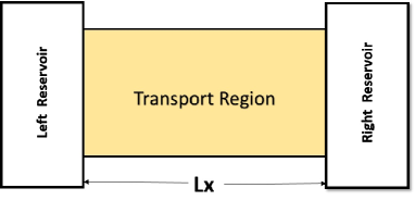
Figure 1: Schematic of the setup under consideration. A finite-size conductor (transport region) is connected to two large reservoirs, which serve as drain and source of the electrical current.

We assume that the conductor is connected to two large reservoirs in regions $x<0$ and $x>L_{x}$, respectively, as shown in Fig. 1. An electric field ${\bf E}(x)=E(x)\hat{\bf e}_{x}$, with $\hat{\bf e}_{x}$ as a unit vector along the $x$ direction, is applied across the sample, and so ${\bf F}=e{\bf E}(x)$. The electric field is confined in the conductor, and satisfies the constraint $V_{\mathrm{L}}-V_{\mathrm{R}}=\int_{0}^{L_{x}}E(x)dx$ with $V_{\mathrm{L}}$ and $V_{\mathrm{R}}$ being the electrical voltages at the left and right ends of the sample. The reservoirs remain in equilibrium, and serve as source and drain of the electrical current, so that the electrical current can flow through the sample continuously. The concrete position dependence of ${\bf E}(x)$ depends on the nonequilibrium charge distribution in the sample. However, we will show that as far as the electrical current is concerned, the result is independent of the profile of ${\bf E}(x)$.

To proceed, it is considered that a stationary transport state has been established, so that $\frac{\partial f}{\partial t}=0$. The electric field is taken to be small, and we linearize the Boltzmann equation, by writing

$$f(\mathbf{k},x)=f_{0}+\left(-\frac{\partial f_{0}}{\partial\varepsilon_{\mathbf{k}}}\right)w(\mathbf{k},x)\ ,$$

where $f_{0}=\frac{1}{e^{(\varepsilon_{\mathbf{k}}-\varepsilon_{\mathrm{F}})/k_{\mathrm{B}}T}+1}$ is the equilibrium Fermi distribution function of the electrons. To the linear order in $E(x)$, the Boltzmann equation reads

$$v_{x}\frac{\partial{w}}{\partial{x}}-v_{x}eE(x)=-\frac{w-\langle w\rangle}{\tau_{0}}\ .$$ (4)

We notice that at low temperatures, $\left(-\frac{\partial f_{0}}{\partial\varepsilon_{\mathbf{k}}}\right)$ is a delta function. Therefore, for all $D=1$, $2$, and $3$ dimensions, the angular momentum average of $\langle\cdots\rangle$ can be expressed in a unified form

$$\left\langle\dots\right\rangle=\frac{\int\dots\left(-\frac{\partial{f_{0}}}{\partial{\varepsilon_{\mathbf{k}}}}\right)d^{\mbox{\tiny{$D$}}}k}{\int\left(-\frac{\partial{f_{0}}}{\partial{\varepsilon_{\mathbf{k}}}}\right)d^{\mbox{\tiny{$D$}}}k}\ .$$ (5)

For right-moving electrons $(v_{x}>0)$, when they just move across the left interface at $x=0$ from the left reservoir into the sample, their distribution function should still be in the equilibrium state, as they have not been accelerated by the electric field. As a result, a boundary condition at the left interface can be written as

$$w(\mathbf{k},x=0^{+})=0\mbox{ }\hskip 28.45274pt(v_{x}>0)\ .\\$$ (6)

For left-moving electrons ($v_{x}<0$), a similar boundary condition exists at the right interface

$$w(\mathbf{k},x=L_{x}-0^{+})=0\mbox{ }\hskip 28.45274pt(v_{x}<0)\ .$$ (7)

We can eliminate the electric field in the Boltzmann equation, using the following transformation

$$w({\bf k},x)=g({\bf k},x)-eV_{\mathrm{L}}+e\int_{0}^{x}E(\xi)d\xi\ .$$ (8)

By substitution of Eq. (8), we derive Eqs. (4), (6) and (7) to be

$$v_{x}\frac{\partial{g}}{\partial{x}}=-\frac{g-\langle g\rangle}{\tau_{0}}\ ,$$ (9)

and

$$g(\mathbf{k},x=0^{+})=eV_{\mathrm{L}}\equiv g_{\mathrm{L}} \mbox{ }(v_{x}>0)\ ,$$ (10)

$$g(\mathbf{k},x=L_{x}-0^{+})=eV_{\mathrm{R}}\equiv g_{\mathrm{R}} \mbox{ }(v_{x}<0)\ .$$ (11)

The electric field $E(x)$ with its profile unknown no longer appears in the Boltzmann equation Eq. (9), and instead, electrical voltages $V_{\mathrm{L}}$ and $V_{\mathrm{R}}$ appear in the boundary conditions Eqs. (10) and (11). It is easy to show that the expression for the electrical current density ${\bf j}$ is invariant under the above transformation, i.e.,

$${\bf j} = \frac{2e}{h^{\mathrm{D}}}\int{{\bf v}w\left(\mathbf{k},x\right)\left(-\frac{\partial f_{0}}{\partial\varepsilon_{\mathbf{k}}}\right)d^{\mbox{\tiny{$D$}}}k}$$

$$\equiv \frac{2e}{h^{\mathrm{D}}}\int{{\bf v}g\left(\mathbf{k},x\right)\left(-\frac{\partial f_{0}}{\partial\varepsilon_{\mathbf{k}}}\right)d^{\mbox{\tiny{$D$}}}k}\ .$$

Therefore, $g({\bf k},x)$ plays the same role as $w({\bf k},x)$ does. We point out that the transformation Eq. (8) is valid in the linear regime, and only in this regime, gauge invariance of the physical quantities calculated from Eqs. (9)-(11), with respect to different choices of the electrical voltages $V_{\mathrm{L}}$ and $V_{\mathrm{R}}$, is guaranteed. The above derivation proves that the electrical current depends only on the electrical voltage difference across the sample, independent of the profile of the electric field $E(x)$. Owing to this finding, laborious calculations of the electric field from the Maxwell’s equations are avoided.

We note that $\langle g\rangle$ is a function of coordinate $x$ only, which will be denoted as $\left\langle g\right\rangle\equiv\bar{g}(x)$ for clarity in the following formulation. According to the definition Eq. (8), $\bar{g}(x)$ describes both the effects of the applied electric field and accumulation of carriers $\langle f\rangle-f_{0}$. From the boundary conditions Eqs. (10) and (11), $\bar{g}(x)$ has the same unit as the chemical potential. Besides, since electric field no longer appears in the Boltzmann equation, and it is the gradient of $\bar{g}(x)$, which drives the electrical current. Therefore, we may call $\bar{g}(x)$ the effective chemical potential (more strictly, change in chemical potential induced by the applied electric field). Eq. (8) may be regarded as a transformation from the representation of charged particles, where the driving force for transport is the electric field, to a representation of neutral particles, where the gradient of the chemical potential causes flow of the particles.

III The exact solution

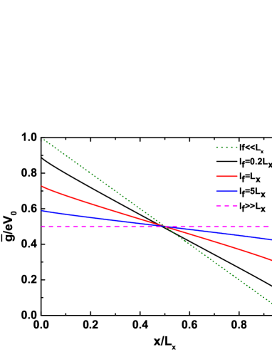
Figure 2: Exact numerical solution of the effective chemical pontential $\bar{g}(x)$ in two dimension as a function of $x/L_{x}$ for some different mean free path to sample length ratios. Here, we choose $V_{\mathrm{L}}=V_{0}$, and $V_{\mathrm{R}}=0$.

A formal solution of $g({\bf k},x)$ can be obtained from the Boltzmann equation Eq. (9) and boundary conditions Eqs. (10) and (11), as a linear functional of $\bar{g}(x)$

$$g({\bf k},x)=\theta(v_{x})\left(g_{\mathrm{L}}e^{-\frac{x}{v_{x}\tau_{0}}}+\int_{0}^{x}e^{-\frac{x-\xi}{v_{x}\tau_{0}}}\bar{g}(\xi)\frac{d\xi}{{v_{x}\tau_{0}}}\right)+\theta(-v_{x})\left(g_{\mathrm{R}}e^{-\frac{x-L_{x}}{v_{x}\tau_{0}}}+\int_{L_{x}}^{x}e^{-\frac{x-\xi}{v_{x}\tau_{0}}}\bar{g}(\xi)\frac{d\xi}{v_{x}\tau_{0}}\right)\ ,$$ (12)

where $\theta(v_{x})$ is the unit step function. By taking the angular momentum average on the both sides of Eq. (12), we obtain a self-consistent integral equation for $\bar{g}(x)$

$$h(x)=\bar{g}(x)-\int_{0}^{x}{K_{1}(x,\xi)\bar{g}(\xi)d\xi}-\int_{L_{x}}^{x}{K_{2}(x,\xi)\bar{g}(\xi)d\xi}\ ,$$ (13)

where

$$h(x)=\left\langle\theta\left(v_{x}\right)g_{\mathrm{L}}e^{-\frac{x}{v_{x}\tau_{0}}}\right\rangle+\left\langle\theta\left(-v_{x}\right)g_{\mathrm{R}}e^{-\frac{x-L_{x}}{v_{x}\tau_{0}}}\right\rangle\ ,$$

$$K_{1}(x,\xi)=\left\langle\theta\left(v_{x}\right)\frac{1}{v_{x}\tau_{0}}e^{-\frac{x-\xi}{v_{x}\tau_{0}}}\right\rangle\ ,$$

$$K_{2}(x,\xi)=\left\langle\theta\left(-v_{x}\right)\frac{1}{v_{x}\tau_{0}}e^{-\frac{x-\xi}{v_{x}\tau_{0}}}\right\rangle\ .$$

Equations (12) and (13) constitute an exact solution to the Boltzmann equation Eq. (9). One can solve the effective chemical potential field $\bar{g}(x)$ from Eq. (13), and then substitute it into Eq. (12) to obtain the nonequilibrium distribution function $g({\bf k},x)$. Once $g({\bf k},x)$ is obtained, the nonequilibrium transport properties of the system can be determined. In general, it is not easy to obtain the exact analytical expression for $\bar{g}(x)$. Before we work out an approximate analytical solution in the next section, we now carry out numerical calculation. Through discretization of the coordinate $x\in[0,L_{x}]$, Eq. (13) is reduced to a set of linear equations, which can be solved numerically. The calculated effective chemical potential field $\bar{g}(x)$ for a two-dimensional sample is plotted in Fig. 2 as a function of $x/L_{x}$ for several different mean free path to sample length ratios. The mean free path is defined as $l_{f}=v_{\mathrm{F}}\tau_{0}$ with $v_{\mathrm{F}}$ being the Fermi velocity. From Fig. 2, we see that $\bar{g}(x)$ is exactly a linear function of $x$ in the two limits $L_{x}\ll l_{f}$ and $L_{x}\gg l_{f}$. In fact, it is easy to obtain from Eq. (13)

$$\bar{g}(x)=\begin{cases}g_{\mathrm{L}}-(g_{\mathrm{L}}-g_{\mathrm{R}})x/L_{x}&\mbox{ }L_{x}\gg l_{f}\\ (g_{\mathrm{L}}+g_{\mathrm{R}})/2&\mbox{ }L_{x}\ll l_{f}\end{cases}\ .$$ (14)

When $L_{x}$ is comparable to $l_{f}$, a linear dependence is still valid in the middle region of the sample, but tiny deviations from the linear dependence occur near the sample boundaries $x=0$ and $x=L_{x}$.

IV An Analytical Approximation

As has been observed in Sec. III, the exact solution of the effective chemical potential $\bar{g}(x)$ is nearly a linear function of coordinate $x$ with negligible deviations occurring near the sample boundaries in the region $L_{x}\sim l_{f}$. Therefore, it is reasonable to make a linear approximation to $\bar{g}(x)$, assuming

$$\bar{g}(x)=a+bx\ ,$$ (15)

with $a$ and $b$ as two constant coefficients to be determined. Substituting this trial solution into Eq. (13), we get an equation for $a$ and $b$

$$\begin{split}0=&\left\langle\theta\left(v_{x}\right)\left(g_{\mathrm{L}}-a+bv_{x}\tau_{0}\right)e^{-\frac{x}{v_{x}\tau_{0}}}\right\rangle+\\ &\left\langle\theta\left(-v_{x}\right)\left(g_{\mathrm{R}}-a-bL_{x}+bv_{x}\tau_{0}\right)e^{-\frac{x-L_{x}}{v_{x}\tau_{0}}}\right\rangle\ .\end{split}$$ (16)

To determine the coefficients $a$ and $b$, one can choose two different values of coordinate $x$ in the above equation to obtain a couple of equations of $a$ and $b$. Noticing that the linear dependence of $\bar{g}(x)$ on $x$ is very well satisfied in the middle region of the sample, we choose $x=\frac{L_{x}}{2}$ and $x=\frac{L_{x}}{2}+\Delta x$, and take the limit $\Delta x\rightarrow 0$ in the final solution. We obtain

$$a =\frac{L_{x}g_{\mathrm{L}}+\kappa l_{f}(g_{\mathrm{{L}}}+g_{\mathrm{R}})}{L_{x}+2\kappa l_{f}}\ ,$$ (17)

$$b =-\frac{g_{\mathrm{L}}-g_{\mathrm{R}}}{L_{x}+2\kappa l_{f}}\ ,$$ (18)

where

$$\kappa=\frac{\tau_{0}\left\langle\theta(v_{x})e^{-\frac{L_{x}}{2v_{x}\tau_{0}}}\right\rangle}{\l_{f}\left\langle\theta(v_{x})\frac{1}{v_{x}}e^{-\frac{L_{x}}{2v_{x}\tau_{0}}}\right\rangle}\ .$$ (19)

Notebaly, Eq. (15) together with Eqs. (17) and (18) recover Eq. (14) in the two limits $L_{x}\gg l_{f}$ and $L_{x}\ll l_{f}$.

IV.1 One Dimension

For $D=1$ dimension, in Eq. (19) $v_{x}\equiv v_{\mathrm{F}}$, and so

$$\kappa\equiv 1\ .$$ (20)

Interestingly, we notice that if we substitute Eqs. (17) and (18) with $\kappa=1$ into Eq. (16), both terms on the right-hand side of Eq. (16) vanish identically for any $x$. This means that for $D=1$, Eq. (15) is actually an exact solution to Eq. (13). Therefore, the conductance formula obtained below for one-dimensional systems is an exact result of the Boltzmann equation. Since the electrical current $I$ is constant along the $x$ direction, we calculate $I$ setting $x=L_{x}/2$, yielding

$$\begin{split}I&=\frac{2e}{h}\int{v_{x}g\left(k_{x},x=\frac{L_{x}}{2}\right)\left(-\frac{\partial f_{0}}{\partial\varepsilon_{k}}\right)dk_{x}}\ \\ &=G^{1\mathrm{D}}(V_{\mathrm{L}}-V_{\mathrm{R}})\ ,\end{split}$$

where

$$G^{1\mathrm{D}}=G_{0}^{1\mathrm{D}}\frac{2l_{f}}{L_{x}+2l_{f}}\ ,$$ (21)

is the conductance of the system. Here, $G_{0}^{1\mathrm{D}}=N_{\mathrm{ch}}\frac{e^{2}}{h}$, with $N_{\mathrm{ch}}=2$ taking into account the spin degeneracy. We note that the electrical current $I$ depends only on the voltage difference $(V_{\mathrm{L}}-V_{\mathrm{R}})$ between the two ends of the sample, which is a manifestation of the gauge invariance. In the ballistic limit $L_{x}\ll l_{f}$, $G^{1\mathrm{D}}=G_{0}^{1\mathrm{D}}$, being consistent with the Landauer-Büttiker formula. In the diffusive limit $L_{x}\gg l_{f}$, $G^{1\mathrm{D}}=\frac{1}{L_{x}}\frac{n_{e}e^{2}\tau_{0}}{m_{e}}$ with $n_{e}=\frac{4k_{\mathrm{F}}}{h}$ as the electron density, which recovers the well-known Boltzmann-Drude formula.

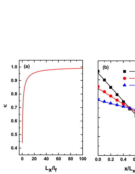
Figure 3: (a) The parameter $\kappa$ as a function of $L_{x}/l_{f}$ in two dimension. (b) The linear approximation to $\bar{g}(x)$ (solid lines), compared with the exact numerical solution reproduced from Fig. 2 (symbols).

IV.2 Two Dimension

In $D=2$ dimension, by using a polar coordinate system, we obtain

$$\kappa=\frac{\int_{-\frac{\pi}{2}}^{\frac{\pi}{2}}e^{-\frac{L_{x}}{2l_{f}\cos\phi}}d\phi}{\int_{-\frac{\pi}{2}}^{\frac{\pi}{2}}\frac{1}{\cos\phi}e^{-\frac{L_{x}}{2l_{f}\cos\phi}}d\phi}\ .$$ (22)

The calculated $\kappa$ is plotted in Fig. 3(a) as a function of $L_{x}/l_{f}$. With increasing $L_{x}/l_{f}$ from $0$, $\kappa$ increases from $0$ and then approaches $1$ rapidly. In Fig. 3(b), the approximate solution $\bar{g}(x)=a+bx$, with $a$ and $b$ given by Eqs. (17) and (18), is plotted as solid lines for some different values of $L_{x}/l_{f}$. The exact solution of $\bar{g}(x)$ is also shown as symbols in Fig. 3(b). The approximate solution fits very well with the exact solution. The electrical current at $x=\frac{L_{x}}{2}$ is calculated, yielding

$$\begin{split}I&=\frac{2eL_{y}}{h^{2}}\int v_{x}g\left({\bf k},x=\frac{L_{x}}{2}\right)\left(-\frac{\partial f_{0}}{\partial\varepsilon_{\mathbf{k}}}\right)dk_{x}dk_{y}\\ &=G^{2\mathrm{D}}(V_{\mathrm{L}}-V_{\mathrm{R}})\ ,\end{split}$$

where

$$G^{2\mathrm{D}}={G}_{0}^{2\mathrm{D}}(\chi^{2\mathrm{D}}_{\mathrm{bal}}+\chi^{2\mathrm{D}}_{\mathrm{dif}})$$ (23)

is the conductance of the two-dimensional sample. Here, $G_{0}^{2\mathrm{D}}=N_{\mathrm{ch}}\frac{e^{2}}{h}$, where $N_{\mathrm{ch}}=\frac{4k_{\mathrm{F}}L_{y}}{h}$ is the channel number with $L_{y}$ as the cross-section length of the sample, and

$$\chi^{\mathrm{2D}}_{\mathrm{bal}}= \frac{\kappa l_{f}}{L_{x}+2\kappa l_{f}}\int_{-\frac{\pi}{2}}^{\frac{\pi}{2}}e^{-\frac{L_{x}}{2l_{f}\cos\phi}}\cos\phi d\phi\ ,$$

$$\chi^{\mathrm{2D}}_{\mathrm{dif}}= \frac{l_{f}}{L_{x}+2\kappa l_{f}}\int_{-\frac{\pi}{2}}^{\frac{\pi}{2}}\left(1-e^{-\frac{L_{x}}{2l_{f}\cos\phi}}\right)\cos^{2}\phi d\phi\ .$$

The total conductance is divided into two parts: ${G}_{0}^{2\mathrm{D}}\chi^{2\mathrm{D}}_{\mathrm{bal}}$ and ${G}_{0}^{2\mathrm{D}}\chi^{2\mathrm{D}}_{\mathrm{dif}}$, standing for contributions from electron ballistic and diffusive transport processes, respectively. In the ballistic limit $L_{x}\ll l_{f}$, $\chi_{\mathrm{bal}}\rightarrow 1$ and $\chi_{\mathrm{dif}}\rightarrow 0$, such that $G^{2\mathrm{D}}=G_{0}^{2\mathrm{D}}$, being consistent with the Landauer-Büttiker formula. In the diffusive limit $L_{x}\gg l_{f}$, $\chi_{\mathrm{bal}}\rightarrow 0$ and $\chi_{\mathrm{dif}}\rightarrow\frac{\pi l_{f}}{2L_{x}}$, and so $G^{2\mathrm{D}}=\frac{L_{y}}{L_{x}}\frac{n_{e}e^{2}\tau_{0}}{m_{e}}$, with $n_{e}=\frac{2\pi k^{2}_{\mathrm{F}}}{h^{2}}$ as the electron density, recovers the Boltzmann-Drude formula.

IV.3 Three Dimension

In $D=3$ dimension, we obtain for $\kappa$

$$\kappa=\frac{\int_{0}^{1}e^{-\frac{L_{x}}{2l_{f}u}}du}{\int_{0}^{1}\frac{1}{u}e^{-\frac{L_{x}}{2l_{f}u}}du}\ .$$ (24)

The conductance is derived to be

$${G}^{3\mathrm{D}}={G}_{0}^{3\mathrm{D}}(\chi_{\mathrm{bal}}^{3\mathrm{D}}+\chi_{\mathrm{dif}}^{3\mathrm{D}})$$ (25)

where ${G}_{0}^{3\mathrm{D}}=N_{\mathrm{ch}}\frac{e^{2}}{h}$ with $N_{\mathrm{ch}}=\frac{2\pi k_{\mathrm{F}}^{2}}{h^{2}}A$ with $A$ as the cross section,

$$\chi^{\mathrm{3D}}_{\mathrm{bal}}= \frac{4\kappa l_{f}}{L_{x}+2\kappa l_{f}}\int_{0}^{1}e^{-\frac{L_{x}}{2l_{f}u}}udu\ ,$$

$$\chi^{\mathrm{3D}}_{\mathrm{dif}}= \frac{4l_{f}}{L_{x}+2\kappa l_{f}}\int_{0}^{1}\left(1-e^{-\frac{L_{x}}{2l_{f}u}}\right)u^{2}du\ .$$

In the ballistic limit $L_{x}\ll l_{f}$, $\chi_{\mathrm{bal}}\rightarrow 1$ and $\chi_{\mathrm{dif}}\rightarrow 0$, and hence $G^{3\mathrm{D}}=G_{0}^{3\mathrm{D}}$, in agreement with the Landauer-Büttiker formula. In the diffusive limit $L_{x}\gg l_{f}$, $\chi_{\mathrm{bal}}\rightarrow 0$ and $\chi_{\mathrm{dif}}\rightarrow\frac{4l_{f}}{3L_{x}}$. As a result, $G^{3\mathrm{D}}=\frac{A}{L_{x}}\frac{n_{e}e^{2}\tau_{0}}{m_{e}}$, with $n_{e}=\frac{8\pi k^{3}_{\mathrm{F}}}{3h^{3}}$ as the electron density, reproduces the Boltzmann-Drude formula.

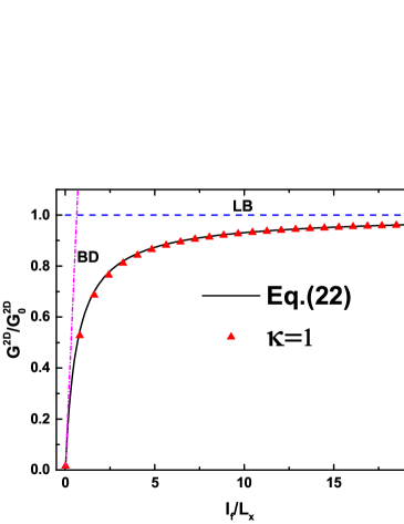
Figure 4: Conductance of a two-dimensional conductor as a function of $l_{f}/L_{x}$ calculated by using the expression Eq. (22) for $\kappa$ (solid line), compared with that calculated by setting $\kappa=1$ (triangles). Dot-dashed line represents the Boltzmann-Drude (BD) formula $G=\frac{n_{e}e^{2}\tau_{0}}{m_{e}}\frac{L_{y}}{L_{x}}$, and the dashed line stands for the Landauer-Büttiker (LB) formula $G=N_{\mathrm{ch}}\frac{e^{2}}{h}$.

We wish to point out that for both $D=2$ and $3$, a further simplification of the theory can be done by setting $\kappa=1$. From Fig. 3(b), we see that $\kappa$ has large deviations from $1$ for $L_{x}\lesssim l_{f}$. Fortunately, as can be seen from Eqs. (23) and (25), the conductance becomes insensitive to the value of $\kappa$ in the region $L_{x}\lesssim l_{f}$. In Fig. 4, the conductance for $D=2$ calculated by using $\kappa=1$ is compared with that obtained by using the expression Eq. (22) for $\kappa$. The difference between them is nearly invisible, an indication that setting $\kappa=1$ is a very good approximation for most purposes.

V A Summary and Discussions

In summary, we have demonstrated that the Boltzmann equation together with proper boundary conditions can describe electron transport properties from diffusive to ballistic regimes. We have worked out a sufficiently accurate analytical solution to the Boltzmann equation. Analytical formulas of the electrical conductance for $D=1$, $2$, and $3$ dimensions are obtained, which smoothly bridge the Boltzmann-Drude formula in diffusive regime and Landauer Büttiker formula in ballistic regime. This simple and intuitive approach can be applied to investigate the effects of sample size and impurity scattering in various charge transport phenomena.

Spin-dependent electronic transport has attracted a great deal of interest in recent years. To describe spin-dependent transport, some essential generalizations of the present theory need to be done. First, a spin relaxation mechanism needs to be included. Second, the effective chemical potential field $\bar{g}({\bf r})$ defined in the present theory includes the effects of the applied electric field and accumulation of particles. In a spin-dependent transport process, while the physical electric field is always spin-independent, the accumulation of particles can become spin-dependent, resulting in the so-called spin accumulation. Therefore, a spin-dependent effective chemical potential field $\bar{g}_{s}({\bf r})$ can be assumed to account for the effect of spin accumulation.

- (1) S. Harris, “An Introduction to the Theory of the Boltzmann Equation,” Dover books, (Courier Corporation, North Chelmsford, 2004).
- (2) C. Cercignani, “The Boltzmann Equation and Its Applications” (Springer, New York, 2012).
- (3) P. Drude, Annalen der Physik 306, 566 (1900); 308, 369 (1900).
- (4) G. D. Mahan, Many-Particle Physics (Plenum, New York, 1990).
- (5) R. Landauer, IBM J. Res. Dev. 1, 223 (1957); Phil. Mag. 21, 863 (1970).
- (6) M. Büttiker, Phys. Rev. Lett. 57, 1761 (1986); Phys. Rev. B 38, 9375 (1988); IBM J. Res. Dev. 32, 317 (1988).
- (7) E. N. Economou, and C. M. Soukoulis, Phys. Rev. Lett. 46, 618 (1981).
- (8) D. S. Fisher, and P. A. Lee, Phys. Rev. B 23, 6851 (1981).
- (9) H. U. Baranger, and A. D. Stone, Phys. Rev. B 40, 8169 (1989).
- (10) E. W. Fenton, Phys. Rev. B 46, 3754 (1992).
- (11) H. M. Pastawski, Phys. Rev. B 44, 6329 (1991).
- (12) Y. Nazarov, and Y. Blanter, “Quantum Transport: Introduction to Nanoscience,” (Cambridge University Press, Cambridge, 2009).
- (13) L. Sheng, D. Y. Xing, Z. D. Wang, and Jinming Dong, Phys. Rev. B 55, 5908 (1997); L. Sheng, H. Y. Teng, D. Y. Xing, 58, 6428 (1998).