Implementation and Performance of FDPS: A Framework for Developing Parallel Particle Simulation Codes

Abstract

We present the basic idea, implementation, measured performance and performance model of FDPS (Framework for developing particle simulators). FDPS is an application-development framework which helps the researchers to develop simulation programs using particle methods for large-scale distributed-memory parallel supercomputers. A particle-based simulation program for distributed-memory parallel computers needs to perform domain decomposition, exchange of particles which are not in the domain of each computing node, and gathering of the particle information in other nodes which are necessary for interaction calculation. Also, even if distributed-memory parallel computers are not used, in order to reduce the amount of computation, algorithms such as Barnes-Hut tree algorithm or Fast Multipole Method should be used in the case of long-range interactions. For short-range interactions, some methods to limit the calculation to neighbor particles are necessary. FDPS provides all of these functions which are necessary for efficient parallel execution of particle-based simulations as “templates”, which are independent of the actual data structure of particles and the functional form of the particle-particle interaction. By using FDPS, researchers can write their programs with the amount of work necessary to write a simple, sequential and unoptimized program of $O(N^{2})$ calculation cost, and yet the program, once compiled with FDPS, will run efficiently on large-scale parallel supercomputers. A simple gravitational $N$-body program can be written in around 120 lines. We report the actual performance of these programs and the performance model. The weak scaling performance is very good, and almost linear speedup was obtained for up to the full system of K computer. The minimum calculation time per timestep is in the range of 30 ms ($N=10^{7}$) to 300 ms ($N=10^{9}$). These are currently limited by the time for the calculation of the domain decomposition and communication necessary for the interaction calculation. We discuss how we can overcome these bottlenecks.

1 Introduction

In the field of computational astronomy, simulations based on particle methods have been widely used. In such simulations, a system is either physically a collection of particles as in the case of star clusters, galaxies and dark-matter halos, or modeled by a collection of particles, as in SPH (smoothed particle hydrodynamics) simulation of astrophysical fluids. Since particles move automatically as the result of integration of the equation of motion of the particle, particle-based simulations have an advantage for systems experiencing strong deformation or systems with high density contrast. This is one of the reasons why particle-based simulations are widely used in astronomy. Examples of particle-based simulations include cosmological simulations or planet-formation simulations with gravitational $N$-body code, simulations of star and galaxy formation with the SPH code or other particle-based codes, and simulations of planetesimal formation with the DEM (discrete element method) code.

We need to use a large number of particles to improve the resolution and accuracy of particle-based simulations, and in order to do so we need to increase the calculation speed and need to use distributed-memory parallel machines efficiently. In other words, we need to implement efficient algorithms such as the Barnes-Hut tree algorithm (Barnes & Hut, 1986), the TreePM algorithm (Xu, 1995) or the Fast Multipole Method (Dehnen, 2000) to distributed-memory parallel computers. In order to achieve high efficiency, we need to divide a computational domain into subdomains in such a way that minimizes the need of communication between processors to maintain the division and to perform interaction calculations. To be more specific, parallel implementations of particle-based simulations contain the following three procedures to achieve the high efficiency: (a) domain decomposition, in which the subdomains to be assigned to computing nodes are determined so that the calculation times are balanced, (b) particle exchange, in which particles are moved to computing nodes corresponding to the subdomains to which they belong, and (c) interaction information exchange, in which each computing node collects the information necessary to calculate the interactions on its particles. In addition, we need to make use of multiple CPU cores in one processor chip and SIMD (single instruction multiple data) execution units in one CPU core, or in some cases GPGPUs (general-purpose computing on graphics processing units) or other accelerators.

In the case of gravitational $N$-body problems, there are a number of works in which the efficient parallelization is discussed (Salmon & Warren, 1994; Dubinski, 1996; Makino, 2004; Ishiyama et al., 2009, 2012). The use of SIMD units is discussed in Nitadori et al. (2006), Tanikawa et al. (2012) and Tanikawa et al. (2013), and GPGPUs in Gaburov et al. (2009), Hamada et al. (2009b), Hamada et al. (2009a), Hamada & Nitadori (2010), Bédorf et al. (2012) and Bédorf et al. (2014).

In the field of molecular dynamics, several groups have been working on parallel implementations. Examples of such efforts include Amber (Case et al., 2015), CHARMM (Brooks et al., 2009), Desmond (Shaw et al., 2014), GROMACS (Abrahama et al., 2014), LAMMPS (Plimpton, 1995), NAMD (Phillips et al., 2005). In the field of CFD (computational fluid dynamics), Many commercial and non-commercial packages now support SPH or other particle-based methods (PAM-CRASH , LS-DYNA , Adventure/LexADV )

Currently, parallel application codes are being developed for each of specific applications of particle methods. Each of these codes requires multi-year effort of a multi-person team. We believe this situation is problematic because of the following reasons.

First, it has become difficult for researchers to try a new method or just a new experiment which requires even a small modification of existing large codes. If one wants to test a new numerical scheme, the first thing he or she would do is to write a small program and to do simple tests. This can be easily done, as far as that program runs on one processor. However, if he or she then wants to try a production-level large calculation using the new method, the parallelization for distributed-memory machines is necessary, and other optimizations are also necessary. However, to develop such a program in a reasonable time is impossible for a single person, or even for a team, unless they already have experiences of developing such a code.

Second, even for a team of people developing a parallel code for one specific problem, it has become difficult to take care of all the optimizations necessary to achieve a reasonable efficiency on recent processors. In fact, the efficiency of many simulation codes mentioned above on today’s latest microprocessors are rather poor, simply because the development team does not have enough time and expertise to implement necessary optimizations (in some case they require the change of data structure, control structure and algorithms).

In our opinion, these difficulties have significantly slowed down researchs in the numerical methods and also the research using large-scale simulations.

We have developed FDPS (Framework for Developing Particle Simulator) (Iwasawa et al., 2015) in order to solve these difficulties. The goal of FDPS is to let researchers concentrate on the implementation of numerical schemes and physics, without spending too much time on parallelization and code optimization. To achieve this goal, we separate a code into domain decomposition, particle exchange, interaction information exchange and fast interaction calculation using Barnes-Hut tree algorithm and/or neighbor search and the rest of the code. We implement these functions as “template” libraries in C++ language. The reason why we use the template libraries is to allow the researchers to define their own data structure for particles and their own functions for particle-particle interactions, and to provide them with highly-optimized libraries with small software overhead. A user of FDPS needs to define the data structure and the function to evaluate particle-particle interaction. Using them as template arguments, FDPS effectively generates the highly-optimized library functions which perform complex operations listed above.

From users’ point of view, what is necessary is to write the program in C++, using FDPS library functions and to compile it using a standard C++ compiler. Using FDPS, users thus can write their particle-based simulation codes for gravitational $N$-body problem, SPH, MD (molecular dynamics), DEM, or many other particle-based methods, without spending their time on parallelization and complex optimization. The compiled code will run efficiently on large-scale parallel machines.

For grid-based or FEM (Finite Element Method) applications, there are many frameworks for developing parallel applications. For example, Cactus (Goodale et al., 2003) has been widely used for numerical relativity, and BoxLib is designed for AMR (adaptive mesh refinement). For particle-based simulations, such frameworks have not been widely used yet, though there were early efforts as in Warren & Salmon (1995), which is limited to long-range, $1/r$ potential. More recently, LexADV_EMPS is currently being developed (Yamada et al., 2015). As its name suggests, it is rather specialized to the EMPS (Explicit Moving Particle Simulation) method (Murotani et al., 2014).

In section 2, we describe the basic design concept of FDPS. In section 3, we describe the implementation of parallel algorithms in FDPS. In section 4, we present the measured performance for three astrophysical applications developed using FDPS. In section 5, we construct a performance model and predict the performance of FDPS on near-future supercomputers. Finally, we summarize this study in section 6.

2 How FDPS works

In this section, we describe the design concept of FDPS. In section 2.1, we present the design concept of FDPS. In section 2.2, we show an $N$-body simulation code written using FDPS, and describe how FDPS is used to perform parallelization algorithms. Part of the contents in this scetion have been published in Iwasawa et al. (2015).

2.1 Design concept

In this section, we present the basic design concept of FDPS. We first present the abstract view of calculation codes for particle-based simulations on distributed-memory parallel computers, and then describe how such abstraction is realized in FDPS.

2.1.1 Abstract view of particle-based simulation codes

In a particle-based simulation code that uses the space decomposition on distributed-memory parallel computers, the calculation proceeds in the following steps:

1. The computational domain is divided into subdomains, and each subdomain is assigned to one MPI process. This step is usually called domain decomposition. Here, minimization of inter-process communication and a good load balance among processes should be achieved.

2. Particles are exchanged among processes, so that each process owns particles in its subdomain. In this paper we call this step particle exchange.

3. Each process collects the information necessary to calculate the interactions on its particles. We call this step interaction-information exchange.

4. Each process calculates interactions between particles in its subdomain. We call this step interaction calculation.

5. The data for each particle are updated using the calculated interactions. This part is done without inter-process communication.

Steps 1, 2, and 3 involve parallelization and inter-process communications. FDPS provides library functions to perform these parts. Therefore, users of FDPS do not have to write the parallelization and/or inter-process communication part of their own code at all.

Step 4 does not involve inter-process communication. However, this step are necessary to perform the actual calculation of interactions between two particles. Users of FDPS should write a simple interaction kernel. The actual interaction calculation using the tree algorithm or neighbor search is done in the FDPS side.

Step 5 involves neither inter-process communication nor interaction calculation. Users of FDPS should and can write their own program for this part.

FDPS can be used to implement particle-based simulation codes for initial value problems which can be expressed as the following ordinary differential equations:

$$\frac{d\vec{u}_{i}}{dt}=\vec{g}\left(\sum_{j}^{N}\vec{f}(\vec{u}_{i},\vec{u}_{j}),\vec{u}_{i}\right).$$ (1)

Here, $N$ is the number of particles in the system, $\vec{u}_{i}$ is a vector which represents the physical quantities of particle $i$, $\vec{f}$ is a function which describes the contribution of particle $j$ to the time derivative of physical quantities of particle $i$, and $\vec{g}$ is a function which converts the sum of the contributions to the actual time derivative. In the case of gravitational $N$-body simulation, $\vec{u}_{i}$ contains position, velocity, mass, and other parameters of particle $i$, $\vec{f}$ is the gravitational force from particle $j$ to particle $i$, and $\vec{g}$ gives velocity as the time derivative of position and calculated acceleration as the time derivative of velocity.

Hereafter, we call a particle that receives the interaction “$i$-particle”, and a particle exerting that interaction “$j$-particle”. The actual contents of vector $\vec{u}_{i}$ and the functional forms of $\vec{f}$ and $\vec{g}$ depend on the physical system and numerical scheme used.

In equation (1) we included only the pairwise interactions, because usually the calculation cost of the pairwise interaction is the highest even when many-body interaction is important. For example, angle and torsion of bonding force in simulation of organic molecules can be done in the user code, with small additional computing cost.

2.1.2 Design concept of FDPS

In this section, we describe how the abstract view presented in the previous section is actually expressed in the FDPS API (application programming interface). The API of FDPS is defined as a set of template library functions in C++ language.

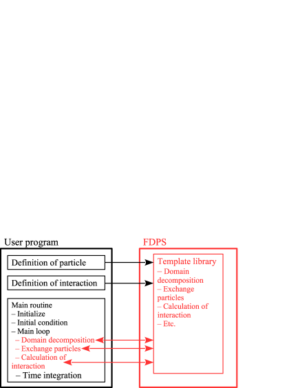
Figure 1: The basic concept of FDPS. The user program gives the definitions of particle and interaction to FDPS, and calls FDPS APIs.

Figure 1 shows how a user program and FDPS library functions interact. The user program gives the definition of a particle $\vec{u}_{i}$ and particle-particle interaction $\vec{f}$ to FDPS at the compile time. They are written in the standard C++ language. Thus, the user program [at least the main() function] currently should be written in C++.

The user program first does the initialization of FDPS library. When the user program is compiled for the MPI environment, the initialization of MPI communication is done in the FDPS initialization function. The setup of the initial condition is done in the user program. It is possible to use file input function defined in FDPS. In the main integration loop, domain decomposition, particle exchange, interaction information exchange and force calculation are all done through library calls to FDPS. The time integration of the physical quantities of particles using the calculated interaction, is done within the user program.

Note that it is possible to implement multi-stage integration schemes such as the Runge-Kutta schemes using FDPS. FDPS can evaluate the right-hand side of equation (1) for a given set of $\vec{u}_{i}$. Therefore, the derivative calculation for intermediate steps can be done by passing $\vec{u}_{i}$ containing appropriate values.

The parallelization using MPI is completely taken care by FDPS, and the use of OpenMP is also taken care by FDPS for the interaction calculation. In order to achieve high performance, the interaction calculation should make efficient use of the cache memory and SIMD units. In FDPS, this is done by requiring an interaction calculation function to calculate the interactions between multiple $i$- and $j$-particles. In this way, the amount of memory access is significantly reduced, since single $j$-particle is used to calculate the interaction on multiple $i$-particles ($i$-particles are also in the cache memory). To make the efficient use of the SIMD execution units, currently the user should write the interaction calculation loop so that the compiler can generate SIMD instructions. Of course, the use of libraries optimized for specific architectures (Nitadori et al., 2006; Tanikawa et al., 2012, 2013) would guarantee very high performance.

It is also possible to use GPUs and other accelerators for the interaction calculation. In order to reduce the communication overhead, so-called “multiwalk” method Hamada et al. (2009b), is implemented. Thus, interaction calculation kernels for accelerators should take multiple sets of the pair of $i$- and $j$-particles. The performance of this version will be discussed elsewhere.

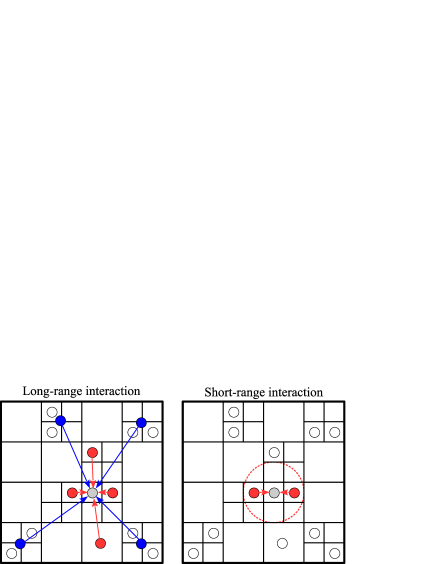
Figure 2: Long-range interaction (left) and short-range interaction (right). Gray, red, and blue points are $i$-particles, $j$-particles, and superparticles, respectively.

As stated earlier, FDPS performs the neighbor search if the interaction is of short-range nature. If the long-range interaction is used, currently FDPS uses the Barnes-Hut tree algorithm. In other words, within FDPS, the distinction between the long-range and short-range interactions is not a physical one but an operational one. If we want to apply the treecode, it is a long-range interaction. Otherwise, it is a short-range interaction. Thus, we can use the simple tree algorithm for pure $1/r$ gravity and the TreePM scheme (Xu, 1995; Bode et al., 2000; Bagla, 2002; Dubinski et al., 2004; Springel, 2005; Yoshikawa & Fukushige, 2005; Ishiyama et al., 2009, 2012) for the periodic boundary.

Figure 2 illustrates the long-range and short-range interactions and how they are calculated in FDPS.

For long-range interactions, Barnes-Hut algorithm is used. Thus, the interactions from a group of distant particles are replaced by that of a superparticle, and equation (1) is modified to

$$\frac{d\vec{u}_{i}}{dt}=\vec{g}\left(\sum_{j}^{N_{\mathrm{J},i}}\vec{f}(\vec{u}_{i},\vec{u}_{j})+\sum_{j^{\prime}}^{N_{\mathrm{S},i}}\vec{f^{\prime}}(\vec{u}_{i},\vec{u^{\prime}}_{j^{\prime}}),\vec{u}_{i}\right),$$ (2)

where $N_{\mathrm{J},i}$ and $N_{\mathrm{S},i}$ are, the number of $j$-particles and superparticles for which we apply multipole-like expansion, the vector $\vec{u^{\prime}}_{j^{\prime}}$ is the physical quantity vector of a superparticle, and the function $\vec{f^{\prime}}$ indicates the interaction exerted on particle $i$ by the superparticle $j^{\prime}$. In simulations with a large number of particles $N$, $N_{\mathrm{J},i}$ and $N_{\mathrm{S},i}$ are many orders of magnitude smaller than $N$. A user need to give functions to construct superparticles from particles and to calculate the interaction from superparticles. Since the most common use of the long-range interaction is for $1/r$ potential, FDPS includes standard implementation of these functions for $1/r$ potential for up to the quadrupole moment.

2.2 An example — gravitational N-body problem

In this section, we present a complete user code for the gravitational $N$-body problem with the open boundary condition, to illustrate how a user write an application program using FDPS. The gravitational interaction is handled as “long-range” type in FDPS. Therefore, we need to provide the data type and interaction calculation functions for superparticles. In order to keep the sample code short, we use the center-of-mass approximation and use the same data class and interaction function for real particles and superparticles.

For the gravitational $N$-body problem, the physical quantity vector $\vec{u}_{i}$ and interaction functions $\vec{f}$, $\vec{f^{\prime}}$, and $\vec{g}$ are given by:

$$\vec{u}_{i} = (\vec{r}_{i},\vec{v}_{i},m_{i}),$$ (3)

$$\vec{f}(\vec{u}_{i},\vec{u}_{j}) = \frac{Gm_{j}\left(\vec{r}_{j}-\vec{r}_{i}\right)}{\left(|\vec{r}_{j}-\vec{r}_{i}|^{2}+\epsilon_{i}^{2}\right)^{3/2}},$$ (4)

$$\vec{f^{\prime}}(\vec{u}_{i},\vec{u^{\prime}}_{j}) = \frac{Gm_{j}^{\prime}\left(\vec{r}_{j}-\vec{r^{\prime}}_{i}\right)}{\left(|\vec{r}_{j}-\vec{r^{\prime}}_{i}|^{2}+\epsilon_{i}^{2}\right)^{3/2}},$$ (5)

$$\vec{g}(\vec{F},\vec{u}_{i}) = (\vec{v}_{i},\vec{F},0),$$ (6)

$$\vec{F} = \sum_{j}\vec{f}(\vec{u}_{i},\vec{u}_{j})+\sum_{j^{\prime}}\vec{f^{\prime}}(\vec{u}_{i},\vec{u^{\prime}}_{j^{\prime}}),\vec{u}_{i},$$ (7)

where $m_{i}$, $\vec{r}_{i}$, $\vec{v}_{i}$, and $\epsilon_{i}$ are, the mass, position, velocity, and gravitational softening of particle $i$, $m_{j}^{\prime}$ and $\vec{r^{\prime}}_{j}$ are, the mass and position of a superparticle $j$, and $G$ is the gravitational constant. Note that the shapes of the functions $\vec{f}$ and $\vec{f^{\prime}}$ are the same.

Listing 2.2 shows the complete code which can be compiled and run, not only on a single-core machine but also massively-parallel, distributed-memory machines such as the K computer. The total number of lines is 117.

⬇

1#include <particle_simulator.hpp>

2using namespace PS;

3

4class Nbody{

5public:

6 F64 mass, eps;

7 F64vec pos, vel, acc;

8 F64vec getPos() const {return pos;}

9 F64 getCharge() const {return mass;}

10 void copyFromFP(const Nbody &in){

11 mass = in.mass;

12 pos = in.pos;

13 eps = in.eps;

14 }

15 void copyFromForce(const Nbody &out) {

16 acc = out.acc;

17 }

18 void clear() {

19 acc = 0.0;

20 }

21 void readAscii(FILE *fp) {

22 fscanf(fp,

23 "%lf%lf%lf%lf%lf%lf%lf%lf",

24 &mass, &eps,

25 &pos.x, &pos.y, &pos.z,

26 &vel.x, &vel.y, &vel.z);

27 }

28 void predict(F64 dt) {

29 vel += (0.5 * dt) * acc;

30 pos += dt * vel;

31 }

32 void correct(F64 dt) {

33 vel += (0.5 * dt) * acc;

34 }

35};

36

37template<class TPJ>

38struct CalcGrav{

39 void operator () (const Nbody * ip,

40 const S32 ni,

41 const TPJ * jp,

42 const S32 nj,

43 Nbody * force) {

44 for(S32 i=0; i<ni; i++){

45 F64vec xi = ip[i].pos;

46 F64 ep2 = ip[i].eps

47 * ip[i].eps;

48 F64vec ai = 0.0;

49 for(S32 j=0; j<nj;j++){

50 F64vec xj = jp[j].pos;

51 F64vec dr = xi - xj;

52 F64 mj = jp[j].mass;

53 F64 dr2 = dr * dr + ep2;

54 F64 dri = 1.0 / sqrt(dr2);

55 ai -= (dri * dri * dri

56 * mj) * dr;

57 }

58 force[i].acc += ai;

59 }

60 }

61};

62

63template<class Tpsys>

64void predict(Tpsys &p,

65 const F64 dt) {

66 S32 n = p.getNumberOfParticleLocal();

67 for(S32 i = 0; i < n; i++)

68 p[i].predict(dt);

69}

70

71template<class Tpsys>

72void correct(Tpsys &p,

73 const F64 dt) {

74 S32 n = p.getNumberOfParticleLocal();

75 for(S32 i = 0; i < n; i++)

76 p[i].correct(dt);

77}

78

79template<class TDI, class TPS, class TTFF>

80void calcGravAllAndWriteBack(TDI &dinfo,

81 TPS &ptcl,

82 TTFF &tree) {

83 dinfo.decomposeDomainAll(ptcl);

84 ptcl.exchangeParticle(dinfo);

85 tree.calcForceAllAndWriteBack

86 (CalcGrav<Nbody>(),

87 CalcGrav<SPJMonopole>(),

88 ptcl, dinfo);

89}

90

91int main(int argc, char *argv[]) {

92 PS::Initialize(argc, argv);

93 F32 time = 0.0;

94 const F32 tend = 10.0;

95 const F32 dtime = 1.0 / 128.0;

96 PS::DomainInfo dinfo;

97 dinfo.initialize();

98 PS::ParticleSystem<Nbody> ptcl;

99 ptcl.initialize();

100 PS::TreeForForceLong<Nbody, Nbody,

101 Nbody>::Monopole grav;

102 grav.initialize(0);

103 ptcl.readParticleAscii(argv[1]);

104 calcGravAllAndWriteBack(dinfo,

105 ptcl,

106 grav);

107 while(time < tend) {

108 predict(ptcl, dtime);

109 calcGravAllAndWriteBack(dinfo,

110 ptcl,

111 grav);

112 correct(ptcl, dtime);

113 time += dtime;

114 }

115 PS::Finalize();

116 return 0;

117}

In the following we describe how this sample code works. It consists of four parts: the declaration to use FDPS (lines 1 and 2), the definition of the particle (the vector $\vec{u}_{i}$) (lines 4 to 35), the definition of the gravitational force (the functions $\vec{f}$ and $\vec{f^{\prime}}$) (lines 37 to 61), and the actual user program. The actual user program consists of a main routine and functions which call library functions of FDPS (lines 63 to line 117). In the following, we discuss each of them.

In order to use FDPS, the user program should include the header file “particle_simulator.hpp”. All functionalities of the standard FDPS library are implemented as the header source library, since they are template libraries which need to receive particle class and interaction functions. FDPS data types and functions are in the namespace “PS”. In this sample program, we declare “PS” as the default namespace to simplify the code. In this sample, however, we did not omit “PS” for FDPS functions and class templates to show that they come from FDPS.

FDPS defines several data types. F32/F64 are data types of 32-bit and 64-bit floating points. S32 is the data type of 32-bit signed integer. F64vec is the class of a vector consisting of three 64-bit floating points. This class provides several operators, such as the addition, subtraction and the inner product indicated by “$*$”. It is not necessary to use these data types in the user program, but some of the functions the user should provide these data types for the return value.

In the second part, the particle data type, (i.e. the vector $\vec{u}_{i}$) is defined as class Nbody. It has the following member variables: mass ($m_{i}$), eps ($\epsilon_{i}$), pos ($\vec{r}_{i}$), vel ($\vec{v}_{i}$), and acc ($d\vec{v}_{i}/dt$). Although the member variable acc does not appear in equation (3) – (7), we need this variable to store the result of the gravitational force calculation. A particle class for FDPS must provide public member functions getPos, copyFromFP, copyFromForce and clear in these names, so that the internal functions of FDPS can access the data within the particle class. For the name of the particle class itself and the names of the member variables, a user can use whatever names allowed by the C++ syntax. The member functions predict and correct are used to integrate the orbits of particles. These are not related to FDPS. Since the interaction is pure $1/r$ type, the construction method for superparticles provided by FDPS can be used and they are not shown here.

In the third part, the interaction functions $\vec{f}$ and $\vec{f^{\prime}}$ are defined. In this example, actually they are the same, except for the class definition for $j$-particles. Therefore, this argument is given as an argument with the template data type TPJ, so that a single source code can be used to generate two functions. The interaction function used in FDPS should have the following five arguments. The first argument ip is the pointer to the array of $i$-particles which receive the interaction. The second argument ni is the number of $i$-particles. The third argument jp is the pointer to the array of $j$-particles or superparticles which exert the interaction. The fourth argument nj is the number of $j$-particles or super-particles. The fifth argument force is the pointer to the array of variables of a user-defined class to which the calculated interactions on $i$-particles can be stored. In this example, we used the particle class itself, but this can be another class or a simple array.

In this example, the interaction function is a function object declared as a struct, with the only member function operator (). FDPS can also accept a function pointer for the interaction function, which would look a bit more familiar to most readers. In this example, the interaction is calculated through a simple double loop. In order to achieve high efficiency, this part should be replaced by a code optimized for specific architectures. In other words, a user needs to optimize just this single function to achieve very high efficiency.

In the fourth part, the main routine and user-defined functions are defined. In the following, we describe the main routine in detail, and briefly discuss other functions. The main routine consists of the following seven steps:

1. Initialize FDPS (line 92).

2. Set simulation time and timestep (lines 93 to 95).

3. Create and initialize objects of FDPS classes (lines 96 to 102).

4. Read in particle data from a file (line 103).

5. Calculate the gravitational forces on all the particles at the initial time (lines 104 to 106).

6. Integrate the orbits of all the particles with Leap-Frog method (lines 107 to 114).

7. Finish the use of FDPS (line 115).

In the following, we describe steps 1, 3, 4, 5, and 7, and skip steps 2 and 6. In step 2, we do not call FDPS libraries. Although we call FDPS libraries in step 6, the usage is the same as in step 5.

In step 1, the FDPS function Initialize is called. In this function, MPI and OpenMP libraries are initialized. If neither of them are used, this function does nothing. All functions of FDPS must be called between this function and the function Finalize.

In step 3, we create and initialize three objects of the FDPS classes:

• dinfo: An object of class DomainInfo. It is used for domain decomposition.

• ptcl: An object of class template ParticleSystem. It takes the user-defined particle class (in this example, Nbody) as the template argument. From the user program, this object looks as an array of $i$-particles.

• grav: An object of data type Monopole defined in class template TreeForForceLong. This object is used for the calculation of long-range interaction using the tree algorithm. It receives three user-defined classes as template arguments: the class to store the calculated interaction, the class for $i$-particles and the class for $j$-particles. In this example, all these three classes are the same as the original class of particles. It is possible to define classes with minimal data for these purposes and use them here, in order to optimize the cache usage. The data type Monopole indicates that the center-of-mass approximation is used for superparticles.

In step 4, the data of particles are read from a file into the object ptcl, using FDPS function readParticleAscii. In this function, a member function of class Nbody, readAscii, is called. Note that the user can write and use his/her own I/O functions. In this case, readParticleAscii is unnecessary.

In step 5, the forces on all particles are calculated through the function calcGravAllAndWriteBack, which is defined in lines 79 to 89. In this function, steps 1 to 4 in section 2.1.1 are performed. In other words, all of the actual work of FDPS libraries to calculate interaction between particles takes place here. For step 1, decomposeDomainAll, a member function of class DomainInfo is called. This function takes the object ptcl as an argument to use the positions of particles to determine the domain decomposition. Step 2 is performed in exchangeParticle, a member function of class ParticleSystem. This function takes the object dinfo as an argument and redistributes particles among MPI processes. Steps 3 and 4 are performed in calcForceAllAndWriteBack, a member function of class TreeForForceLong. This function takes the user-defined function object CalcGrav as the first and second arguments, and calculates particle-particle and particle-superparticle interactions using them.

In step 7, the FDPS function Finalize is called. It calls the MPI_Finalize function.

In this section, we have described in detail how a user program written using FDPS looks like. As we stated earlier, this program can be compiled with or without parallelization using MPI and/or OpenMP, without any change in the user program. The executable parallelized with MPI is generated by using an appropriate compiler with MPI support and a compile-time flag. Thus, a user need not worry about complicated bookkeeping necessary for parallelization using MPI.

In the next section, we describe how FDPS provides a generic framework which takes care of parallelization and bookkeeping for particle-based simulations.

3 Implementation

In this section, we describe how the operations discussed in the previous section are implemented in FDPS. In section 3.1 we describe the domain decomposition and particle exchange, and in section 3.2, the calculation of interactions. Part of the contents in this scetion have been published in Iwasawa et al. (2015).

3.1 Domain decomposition and particle exchange

In this section, we describe how the domain decomposition and the exchange of particles are implemented in FDPS. We used the multisection method (Makino, 2004) with the so-called sampling method (Blackston & Suel, 1997). The multisection method is a generalization of ORB (Orthogonal Recursive Bisection). In ORB, as its name suggests, bisection is applied to each coordinate axis recursively. In multisection method, division in one coordinate is not to two domains but to an arbitrary number of domains. Since one dimension can be divided to more than two sections, it is not necessary to apply divisions many times. So we apply divisions only once to each coordinate axis. A practical advantage of this method is that the number of processors is not limited to powers of two.

Figure 3 illustrates an example of the multisection method with $(n_{x},n_{y},n_{z})=(7,6,1)$. We can see that the size and shape of subdomains show large variation. By allowing this variation, FDPS achieves quite good load balance and high scalability. Note that $n=n_{x}n_{y}n_{z}$ is the number of MPI processes. By default, values of $n_{x}$, $n_{y}$, and $n_{z}$ are chosen so that they are integers close to $n^{1/3}$. For figure  3, we force the numbers used to make a two-dimensional decomposition.

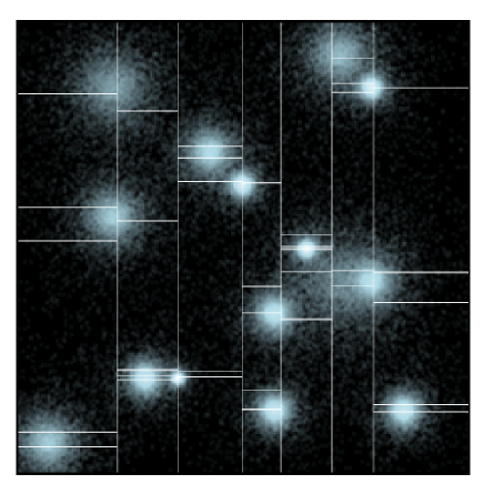
Figure 3: Example of the domain decomposition. The division is $7\times 6$ in 2-dimension.

In the sampling method, first each process performs random sampling of particles under it, and sends them to the process with rank 0 (“root” process hereafter). Then the root process calculates the division so that sample particles are equally divided over all processes, and broadcasts the geometry of domains to all other processes. In order to achieve good load balance, sampling frequency should be changed according to the calculation cost per particle (Ishiyama et al., 2009).

The sampling method works fine, if the number of particles per process is significantly larger than the number of process. This is, however, not the case for runs with a large number of nodes. When the number of particles per process is not much larger than the number of processes, the total number of sample particles which the root process needs to handle exceeds the number of particles per process itself, and thus calculation time of domain decomposition in the root process becomes visible.

In order to reduce the calculation time, we also parallelized the domain decomposition, currently in the direction of $x$ axis only. The basic idea is that each node sends the sample particles not to the root process of the all MPI processes but to the processes with index $(i,0,0)$. Then processes $(i,0,0)$ sort the sample particles and exchange the number of sample particles they received. Using these two pieces of information, each of $(i,0,0)$ processes can determine all domain boundaries inside its current domain in the $x$ direction. Thus, they can determine which sample particles should be sent to where. After the exchange of sample particles, each of $(i,0,0)$ processes can determine the decompositions in $y$ and $z$ directions.

A naive implementation of the above algorithm requires “global” sorting of sample particles over all of $(i,0,0)$ processes. In order to simplify this part, before each process sends the sample particles to $(i,0,0)$ processes, they exchange their samples with other processes with the same location in $y$ and $z$ process coordinates, so that they have sample particles in the current domain decomposition in the x direction. As a result, particles sent to $(i,0,0)$ processes are already sorted at the level of domains decomposition in $x$ direction, and we need only the sorting within each of $(i,0,0)$ processes to obtain the globally sorted particles.

Thus, our implementation of parallelized domain decomposition is as follows:

1. Each process samples particles randomly from its own particles. In order to achieve an optimal load balance, the sampling rate of particles is changed so that it is proportional to the CPU time per particle spent on that process (Ishiyama et al., 2009). FDPS provides several options including this optimal balance.

2. Each process exchanges the sample particles according to the current domain boundary in the $x$ direction with the process with the same y and z indices, so that they have sample particles in the current domain decomposition in the $x$ direction.

3. Each process with index $(i,y,z)$ sends the sample particles to the process with index $(i,0,0)$, in other words, the root processes in each of $y$-$z$ planes collects subsamples.

4. Each root process sorts the sample particles in the $x$ direction. Now, the sample particles are sorted globally in the $x$ direction.

5. Each root process sends the number of the sample particles to the other root processes and determines the global rank of the sample particles.

6. Determine the $x$ coordinate of new domains by dividing all sample particles into $n_{x}$ subsets with equal number of sample particles.

7. Each root process exchanges sample particles with other root processes, so that they have the sample particles in new domain in the $x$ direction.

8. Each root process determines the $y$ and $z$ coordinates of new domains.

9. Each root process broadcasts the geometries of new domains to all other processes.

It is also possible to parallelize the determination of subdomains in step 8, but even for the full-node runs on K computer we found the current parallelization is sufficient.

For particle exchange and also for interaction information exchange, we use MPI_Alltoall to exchange the length of the data and MPI_Isend and MPI_Irecv to actually exchange the data. At least on K computer, we found that the performance of vendor-provided MPI_Alltoall is not optimal for short messages. We implemented a hand-crafted version in which the messages sent to the same relay points are combined in order to reduce the total number of messages.

After the domain decomposition is done and the result is broadcasted to all processes, they exchange particles so that each of them has particles in its domain. Since each process has the complete information of the domain decomposition, this part is pretty straightforward to implement. Each process looks at each of its particles, and determines if that particle is still in its domain. If not, the process determines to which process that particle should be sent. After the destinations of all particles are determined, each process sends them out, using MPI_Isend and MPI_Irecv functions.

3.2 Interaction calculation

In this section, we describe the implementations of interaction information exchange and actual interaction calculation. In the interaction information exchange step, each process sends the data required by other nodes. In the interaction calculation step, actual interaction calculation is done using the received data. For both steps, the Barnes-Hut octree structure is used, for both of long- and short-range interactions.

First, each process constructs the tree of its local particles. Then this tree is used to determine the data to be sent to other processes. For the long-range interaction, the procedure is the same as that for usual tree traversal(Barnes & Hut, 1986; Barnes, 1990). The tree traversal is used also for short-range interactions. FDPS can currently handle four different types of the cutoff length for the short-range interactions: fixed, $j$-dependent, $i$-dependent and symmetric. For $i$-dependent and symmetric cutoffs, the tree traversal should be done twice.

Using the received data, each process performs the force calculation. To do so, it first constructs the tree of all data received and local particles, and then uses it to calculate the interaction on local particles.

4 Performance of applications developed using FDPS

In this section, we present the performance of three astrophysical applications developped using FDPS. One is the pure gravity code with open boundary applied to disk galaxy simulation. The second one is again pure gravity application but with periodic boundary applied to cosmological simulation. The third one is gravity + SPH calculation applied to the giant impact (GI) simulation. For the performance measurement, we used two systems. One is K computer of RIKEN AICS, and the other is Cray XC30 of CfCA, National Astronomical Observatory of Japan. K computer consists of 82,944 Fujitsu SPARC64 VIIIfx processors, each with eight cores. The theoretical peak performance of one core is 16 Gflops, for both of single- and double-precision operations. Cray XC30 of CfCA consists of 1060 nodes, or 2120 Intel Xeon E5-2690v3 processors (12 cores, 2.6GHz). The theoretical peak performance of one core is 83.2 and 41.6 Gflops for single- and double-precision operations, respectively. In all runs on K computer, we use the hybrid MPI-OpenMP mode of FDPS, in which one MPI process is assigned to one node. On the other hand, for XC30, we use the flat MPI mode of FDPS. The source code is the same except for that for the interaction calculation functions. The interaction calculation part was written to take full advantage of the SIMD instruction set of the target architecture, and thus written specifically for SPARC64 VIIIfx (HPC-ACE instruction set) and Xeon E5 v3 (AVX2 instruction set).

4.1 Disk galaxy simulation

In this section, we discuss the performance and scalability of a gravitational $N$-body simulation code implemented using FDPS. Some results in this scetion have been published in Iwasawa et al. (2015). The code is essentially the same as the sample code described in section 2.2, except for the following two differences in the user code for the calculation of the interaction. First, to improve the accuracy, we used the expansion up to the quadrupole moment, instead of the monopole-only one used in the sample code. Second, we used the highly optimized kernel developed using SIMD builtin functions, instead of the simple one in the sample code.

We apply this code for the simulation of the Milky Way-like galaxy, which consists of a bulge, a disk, and a dark matter halo. For examples of recent large-scale simulations, see Fujii et al. (2011) and Bédorf et al. (2014).

The initial condition is the Milky Way model, which is the same as that in Bédorf et al. (2014). The mass of the bulge is $4.6\times 10^{9}M_{\odot}$, and it has a spherically-symmetric density profile of the Hernquist model (Hernquist, 1990) with the half-mass radius of $0.5$ kpc. The disk is an axisymmetric exponential disk with the scale radius of $3$ kpc, the scale height of $200$ pc and the mass $5.0\times 10^{10}M_{\odot}$. The dark halo has an Navarro-Frenk-White (NFW) density profile (Navarro et al., 1996) with the half-mass radius of $40$ kpc and the mass of $6.0\times 10^{11}M_{\odot}$. In order to realize the Milky Way model, we used GalacticICS (Widrow & Dubinski, 2005). For all simulations in this section, we adopt $\theta=0.4$ for the opening angle for the tree algorithm. We set the average number of particles sampled for the domain decomposition to 500.

Figure 4 illustrates the time evolution of the bulge and disk in the run with $512$ nodes on the K computer. The disk is initially axisymmetric. We can see that spiral structure develops (0.5 and 1 Gyrs) and a central bar follows the spiral (1 Gyrs and later). As the bar grows, the two-arm structure becomes more visible (3 Gyrs).

Figure 4: Face-on surface density maps of the bulge and disk.

Figure 5 shows the measured weak-scaling performance. We fixed the number of particles per core to 266,367 and measured the performance for the number of cores in the range of 4096 to 663,552 on the K computer, and in the range of 32 to 2048 on XC30. We can see that the measured efficiency and scalability are both very good. The efficiency is more than 50% for the entire range of cores on the K computer. The efficiency of XC30 is a bit worse than that of the K computer. This difference comes from the difference of two processors. The Fujitsu processor showed higher efficiency, while the Intel processor has 5.2 times higher peak performance per core. We can see that the time for domain decomposition increase as we increase the number of cores. The slope is around 2/3 as can be expected from our current algorithm discussed in section 3.1.

Figure 6 shows the measured strong-scaling performance. We fixed the total number of particles to $550$ million and measured the performance for 512 to 32768 cores on K computer and 256 to 2048 cores on XC30. We can also see the measured efficiency and scalability are both very good, for the strong-scaling performance.

Bédorf et al. (2014) reported the wallclock time of 4 seconds for their 27-billion particle simulation on the Titan system with 2048 NVIDIA Tesla K20X, with the theoretical peak performance of 8PF (single precision, since the single precision was used for the interaction calculation). This corresponds to 0.8 billion particles per second per petaflops. Our code on K computer requires 15 seconds on 16384 nodes (2PF theoretical peak), resulting in 1 billion particles per second per petaflops. Therefore, we can conclude that our FDPS code achieved the performance slightly better than one of the best codes specialized to gravitational $N$-body problem.

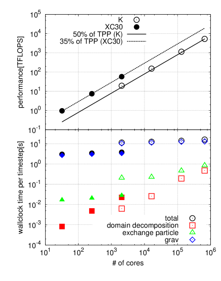
Figure 5: Weak-scaling performance of the gravitational $N$ body code. The speed of the floating-point operation (top) and wallclock time per one timestep (bottom) are plotted as functions of the number of cores. Open and filled symbols indicate the performances of K computer and cray XC30, respectively. In the top panel, the solid line indicates 50% of the theoretical peak performance of K computer and the dotted line indicates 35% of the theoretical peak performance of XC30. In the bottom panel, time spent for the interaction calculation (diamond), the domain decomposition (square) the exchange particles (triangle) are also shown.

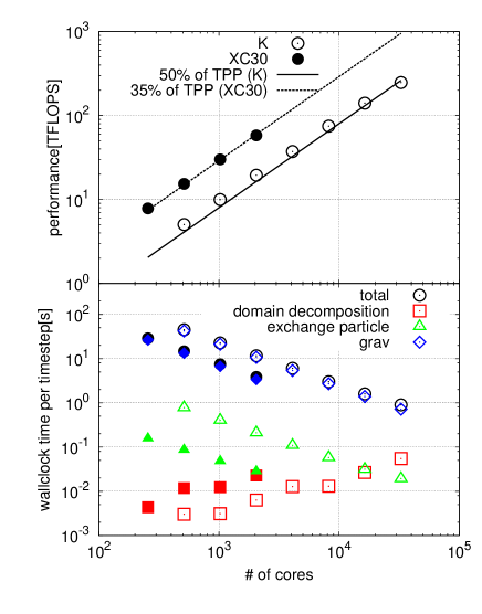
Figure 6: The same figure as figure 5 but for the strong-scaling performance for 550 million particles

4.2 Cosmological simulation

In this section, we discuss the performance of a cosmological simulation code implemented using FDPS. We implemented TreePM (Tree Particle-Mesh) method and measured the performance on XC30. Our TreePM code is based on the code developed by K. Yoshikawa. The Particle-Mesh part of the code was developed by Ishiyama et al. (2012) and this code is included in the FDPS package as an external module.

We initially place particles uniformly in a cube and gave them zero velocity. For the calculation of the tree force , we used a monopole only kernel with cutoff. The cutoff length of the force is three times larger than the width of the mesh. We set $\theta$ to 0.5. For the calculation of the mesh force, the mass density is assigned to each of the grid points, using the triangular shaped cloud scheme and the density profile we used is the S2 profile (Hockney & Eastwood, 1988).

Figures 7 and 8 show the weak and strong scaling performance, respectively. For the weak-scaling measurement, we fixed the number of particles per process to 5.73 million and measured the performance for the number of cores in the range of 192 to 12000 on XC30. For the strong-scaling measurements, we fixed the total number of particles to $2048^{3}$ and measured the performance for the number of cores in the range of 1536 to 12000 on XC30. We can see that the time for the calculation of the tree force is dominant and both of the weak and strong scalings are good except for the very large number of cores (12000) for the strong scaling measurement. One reason is that the scalability of the calculation of the mesh force is not very good. Another reason is that the time for the domain decomposition grows linearly for large number of cores, because we did not use parallelized domain decomposition here. The efficiency is 7% of the theoretical peak performance. It is rather low compared to that for the disk galaxy simulations in section 4.1. The main reason is that we use a lookup table for the force calculation. If we evaluate the force without the lookup table, the nominal efficiency would be much better, but the total time would be longer.

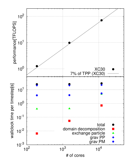
Figure 7: Weak-scaling performance of the TreePM code. The speed of the floating-point operation (top) and wallclock time per one timestep (bottom) are plotted as functions of the number of cores. In the top panel, the solid line indicates 7% of the theoretical peak performance of XC30. In the bottom panel, time spent for the Particle-Particle interaction calculation (diamond), the Particle-Mesh interaction (pentagon), the domain decomposition (square) and the exchange particles (triangle) are also shown.

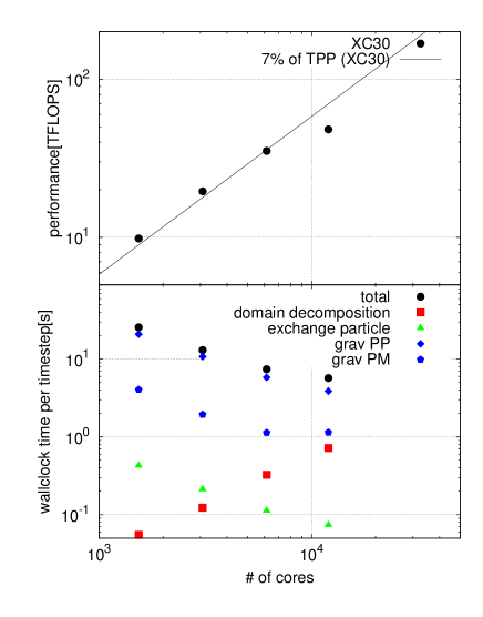
Figure 8: The same as figure 7 but for the strong-scaling performance. In this case, the number of particles is $2048^{3}$.

4.3 Giant impact simulation

In this section, we discuss the performance of an SPH simulation code with self-gravity implemented using FDPS. Some results in this scetion have been published in Iwasawa et al. (2015). The test problem used is the simulation of GI. The GI hypothesis (Hartmann & Davis, 1975; Cameron & Ward, 1976) is one of the most popular scenarios for the formation of the Moon. The hypothesis is as follows. About 5 billion years ago, a Mars-sized object (hereafter, the impactor) collided with the proto-Earth (hereafter, the target). A large amount of debris was scattered, which first formed the debris disk and eventually the Moon. Many researchers have performed simulations of GI, using the SPH method (Benz et al., 1986; Canup et al., 2013; Asphaug & Reufer, 2014).

For the gravity, we used monopole-only kernel with $\theta=0.5$. We adopt the standard SPH scheme (Monaghan, 1992; Rosswog, 2009; Springel, 2010) for the hydro part. Artificial viscosity is used to handle shocks (Monaghan, 1997), and the standard Balsara switch is used to reduce the shear viscosity (Balsara, 1995). A kernel function we used is the Wendland $C^{6}$ and the cutoff radius is 4.2 times larger than the local mean inter-particle distance. In other words, each particle interact with about 300 particles. This neighbor number is the appropriate for this kernel to avoid the pairing instability (Dehnen & Aly, 2012).

Assuming that the target and impactor consist of granite, we adopt equation of state of granite (Benz et al., 1986) for the particles. For the initial condition, we assume the parabolic orbit with the initial angular momentum 1.21 times of the current Earth-Moon system.

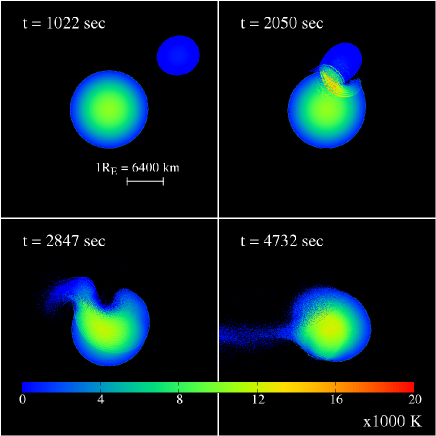
Figure 9: Temperature maps of the target and impactor in the run with $9.9$ million particles at four different epochs.

Figure 9 shows the time evolution of the target and impactor for a run with 9.9 million particles. We can see that the shocks are formed just after the moment of impact in both the target and impactor ($t=2050$ sec). The shock propagates in the target, while the impactor is completely disrupted ($t=2847$ sec) and debris are ejected. A part of the debris falls back to the target, while the rest will eventually form the disk and the Moon. So far, the resolution used in the published papers have been much lower. We plan to use this code to improve the accuracy of the GI simulations.

Figure 10 and 11 show the measured weak and strong scaling performance. For the weak-scaling measurement, we fixed the number of particles per core to 20,000 and measured the performance for the number of cores in the range of 256 to 131,072 on the K computer. On the other hand, for the strong-scaling measurement, we fixed the total number of particles to $39$ million and measured the performance for the number of cores in the range of 512 to 16,384 on K computer. We can see that the performance is good even for very large number of cores. The efficiency is about 40% of the theoretical peak performance. The hydro part consumes more time than the gravity part does, mainly because the particle-particle interaction is more complicated.

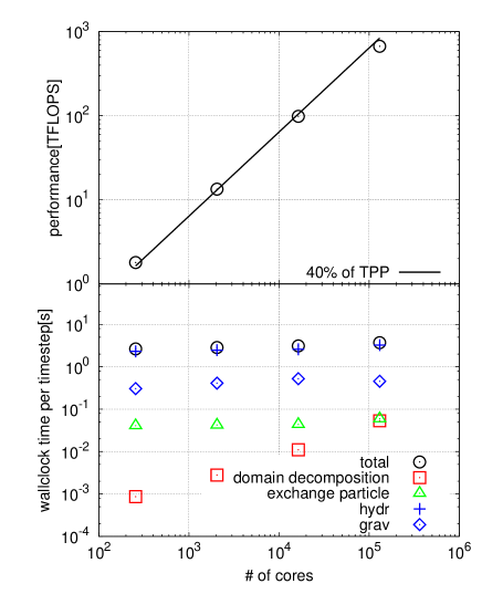
Figure 10: Weak-scaling performance of the SPH code. The speed of the floating-point operation (top) and wallclock time per one timestep (bottom) are plotted as functions of the number of cores. In the top panel, the solid line indicates 40% of the theoretical peak performance of K computer. In the bottom panel, time spent for the hydrodynamics calculation (cross), the gravity calculation (diamond), the domain decomposition (square) the exchange particles (triangle) are also shown.

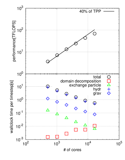
Figure 11: The same as figure 10 but for the strong-scaling performance for $39$ million particles.

5 Performance model

In this section, we present the performance model of applications implemented using FDPS. As described in section 2, the calculation of a typical application written using FDPS proceeds in the following steps

1. Update the domain decomposition and exchange particles accordingly (not in every timestep).

2. Construct the local tree structure and exchange particles and superparticles necessary for interaction calculation.

3. Construct the “global” tree.

4. Perform the interaction calculation.

5. Update the physical quantities of particles using the calculated interactions.

In the case of complex applications which require more than one interaction calculations, each of the above steps, except for the domain decomposition, may be executed more than one time per one timestep.

For a simple application, thus, the total wallclock time per one timestep should be expressed as

$$T_{\rm step}=T_{\rm dc}/n_{\rm dc}+T_{\rm lt}+T_{\rm exch}+T_{\rm icalc}+T_{\rm misc},$$ (8)

where $T_{\rm dc}$, $T_{\rm lt}$, $T_{\rm exch}$, $T_{\rm icalc}$, and $T_{\rm misc}$ are the times for domain composition and particle exchange, local tree construction, exchange of particles and superparticles for interaction calculation, interaction calculation, and other calculations such as particle update, respectively. The term $n_{\rm dc}$ is the interval at which the domain decomposition is performed.

In the following, we first construct the model for the communication time. Then we construct models for each term of the right hand side of equation 8, and finally we compare the model with the actual measurement presented in section 5.6.

5.1 Communication model

What ultimately determines the efficiency of a calculation performed on a large-scale parallel machine is the communication overhead. Thus, it is very important to understand what types of communication would take what amount of time on actual hardware. In this section, we summarize the characteristics of the communication performance of K computer.

In FDPS, almost all communications are through the use of collective communications, such as MPI_Allreduce, MPI_Alltoall, and MPI_Alltoallv. However, measurement of the performance of these routines for uniform message length is not enough, since the amount of data to be transferred between processes generally depends on the physical distance between domains assigned to those processes. Therefore, we first present the timing results for simple point-to-point communication, and then for collective communications.

Figure 12 shows the elapsed time as the function of the message length, for point-to-point communication between “neighboring” processes. In the case of K computer, we used three-dimensional node allocation, so that “neighboring” processes are actually close to each other in its torus network.

We can see that the elapsed time can be fitted reasonably well as

$$T_{\rm p2p}=T_{\rm p2p,startup}+n_{\rm word}T_{\rm p2p,word},$$ (9)

where $T_{\rm p2p,startup}$ is the startup time which is independent of the message length and $T_{\rm p2p,word}$ is the time to transfer one byte of message. Here, $n_{\rm word}$ is the length of the message in units of bytes. On K computer, $T_{\rm p2p,startup}$ is 0.0101 ms and $T_{\rm p2p,word}$ is $2.11\times 10^{-7}$ ms per byte. For a short message, there is a rather big discrepancy between the analytic model and measured points, because for short messages K computer used several different algorithms.

Figure 12: Elapsed time for point-to-point communication as a function of size of message measured on K computer.

Figure 13 shows the elapsed times for MPI_Alltoallv. The number of processes $n_{p}$ is 32 to 2048. They are again modeled by the simple form

$$T_{\rm alltoallv}=T_{\rm alltoallv,\rm startup}+n_{\rm word}T_{\rm alltoallv,\rm word},$$ (10)

where $T_{\rm\rm alltoallv,\rm startup}$ is the startup time and $T_{\rm alltoallv,\rm word}$ is the time to transfer one byte of message. We list these values in table 1.

Table 1: Time coefficients in equation (10)

	$n_{p}=32$	$n_{p}=256$	$n_{p}=2048$
$T_{\rm alltoallv,startup}$ [ms]	0.103	0.460	2.87
$T_{\rm alltoallv,word}$ [ms/byte]	$8.25\times 10^{-6}$	$9.13\times 10^{-5}$	$1.32\times 10^{-3}$

The coefficients themselves in equation (10) depend on the number of MPI processes $n_{p}$, as shown in figures 14. They are modeled as

$$T_{\rm alltoallv,startup} = \tau_{\rm alltoallv,startup}n_{p},$$ (11)

$$T_{\rm alltoallv,word} = \tau_{\rm alltoallv,word}n_{p}^{4/3}.$$ (12)

Here we assume that the speed to transfer message using MPI_Alltoallv is limited to the bisection bandwidth of the system. Under this assumption, $T_{\rm alltoallv,word}$ should be proportional to $n_{p}^{4/3}$. To estimate $\tau_{\rm alltoallv,startup}$ and $\tau_{\rm alltoallv,word}$, we use measurements for message sizes of 8 bytes and 32k bytes. In K computer, we found that $\tau_{\rm alltoallv,startup}$ is $0.00166$ ms and $\tau_{\rm alltoallv,word}$ is $1.11\times 10^{-7}$ ms per byte. If MPI_Alltoallv is limited to the bisection bandwidth in K computer, $\tau_{\rm alltoallv,word}$ would be $5\times 10^{-8}$ ms per byte. We can see that the actual performance of MPI_Alltoallv on K computer is quite good.

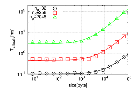
Figure 13: Elapsed time of MPI_Alltoallv as a function of message size measured on K computer.

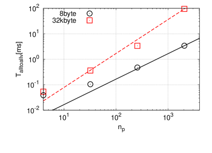
Figure 14: Elapsed time of MPI_Alltoallv to send messeage of 8 bytes (circles) and 32k bytes (squares) as a function of the number of processes measured on K computer. Solid and dashed curves indicate the results for the message size of 8 bytes and 32k bytes, respectively.

5.2 Domain decomposition

For the hierarchical domain decomposition method described in section 3.1, the calculation time is expressed as

$$T_{\rm dc}=T_{\rm dc,gather}+T_{\rm dc,sort}+T_{\rm dc,exch}+T_{\rm dc,misc},$$ (13)

where $T_{\rm dc,gather}$ is the time for the $(i,0,0)$ process to collect sample particles, $T_{\rm dc,sort}$ is the time to sort sample particles on the $(i,0,0)$ process, $T_{\rm dc,exch}$ is the time to exchange particles after the new domains are determined, and $T_{\rm dc,misc}$ is the time for remaining procedures such as initial exchange of samples in $x$ direction, exchange of sample particles and domain boundaries in $x$ direction, and broadcasting of the domain boundaries in $y$-$z$ planes.

On the machines we so far tested, $T_{\rm dc,gather}$ and $T_{\rm dc,misc}$ are much smaller than $T_{\rm dc,sort}$ and $T_{\rm dc,exch}$. Therefore we consider these two terms only.

First, we consider the time to sort sample particles. Since we use the quick sort, the term $T_{\rm dc,sort}$ is expressed as

$$T_{\rm dc,sort} = \tau_{\rm sort}\left[2n_{\rm smp}n_{y}n_{z}{\rm log}(n_{\rm smp}n_{y}n_{z})+n_{y}n_{\rm smp}n_{z}{\rm log}(n_{\rm smp}n_{z})\right]$$ (14)

$$\sim \tau_{\rm dc,sort}n_{\rm smp}n_{p}^{2/3},$$ (15)

where $n_{\rm smp}$ is the average number of sample particles per process, and $n_{x}$, $n_{y}$ and $n_{z}$ are the numbers of processes in x, $y$ and $z$ direction. Here, $\tau_{\rm dc,sort}\sim{\rm log}(n_{\rm smp}^{3}n_{p}^{5/3})\tau_{\rm sort}$. The first term expresses the time to sort samples in $y$-$z$ planes with respect to $x$ and $y$ directions. The second term expresses that time to sort samples respect to $z$ direction.

In order to model $T_{\rm dc,exch}$, we need to model the number of particles which moves from one domain to another. This number would depend on various factors, in particular the nature of the system we consider. For example, if we are calculating the early phase of the cosmological structure formation, particles do not move much in a single timestep, and thus the number of particles moved between domains is small. On the other hand, if we are calculating single virialized self-gravitating system, particles move a relatively large distances (comparable to average interparticle distance) in a single timestep. In this case, if one process contains $n$ particles, half of particles in the “surface” of the domain might migrate in and out the domain. Thus, $O(n^{2/3})$ particles could be exchanged in this case.

Figures 15, 16 and 17 show the elapsed time for sorting samples, exchanging samples, and domain decomposition for the case of disk galaxy simulations in the case of $n_{\rm smp}=500$ and $n\sim 5.3\times 10^{5}$. We also plot the analytic models given by

$$T_{\rm dc} \sim T_{\rm dc,sort}+T_{\rm dc,exch}$$ (16)

$$= \tau_{\rm dc,sort}n_{\rm smp}n_{p}^{2/3}+\tau_{\rm dc,exch}\sigma\Delta t/\left<r\right>n^{2/3}b_{p},$$ (17)

where $\tau_{\rm dc,sort}$ and $\tau_{\rm dc,exch}$ are the execution time for sorting one particle and for exchanging one particle respectively, $\sigma$ is the typical velocity of particles, $\Delta t$ is the timestep and $\left<r\right>$ is the average interparticle distance. For simplicity we ignore weak log term in $T_{\rm dc,sort}$ . On K computer, $\tau_{\rm dc,sort}=2.67\times 10^{-7}$ second and $\tau_{\rm dc,exch}=1.42\times 10^{-7}$ second per byte. Note that $\tau_{\rm dc,exch}\sim 672T_{\rm p2p,word}$.

In figure 16, for small $n_{p}$, the analytic model gives the value about 2 times smaller than the measured point. This is because the measured values include not only the time to exchange particles but also the time to determine appropriate processes to send particles, while the analytic model includes only the time to exchange particles. For small $n_{p}$, the time to determine the appropriate process is not negligible, and therefor the analytic model gives an underestimate.

Figure 15: Measured $T_{\rm dc,sort}$ and its analytic model as a function of $n_{p}$, in the case of $n_{\rm smp}=500$ and $n\sim 5.3\times 10^{5}$.

Figure 16: Measured $T_{\rm dc,exch}$ and its analytic model as a function of $n_{p}$, in the case of $n_{\rm smp}=500$ and $n\sim 5.3\times 10^{5}$.

Figure 17: Measured $T_{\rm dc}$ and its analytic model as a function of $n_{p}$, in the case of $n_{\rm smp}=500$ and $n\sim 5.3\times 10^{5}$.

The analysis above, however, indicates that $T_{\rm dc,exch}$ is, even when it is relatively large, still much smaller than $T_{\rm exch}$, which is the time to exchange particles and superparticles for interaction calculation (see section 5.4).

5.3 Tree construction

Theoretically, the cost of tree construction is $O(n{\rm log}n)$, and of the same order as the interaction calculations itself. However, in our current implementation, the interaction calculation is much more expensive, independent of target architecture and the type of the interaction. Thus we ignore the time for the tree constructions.

5.4 Exchange of particles and superparticles

For the exchange of particles and superparticles, in the current implementation of FDPS, first each node constructs the list of particles and superparticles (hereafter the exchange list) to be sent to all other nodes, and then data are exchanged through a single call to MPI_Alltoallv. The way the exchange list is constructed depends on the force calculation mode. In the case of long-range forces, usual tree traversal with a fixed opening angle $\theta$ is performed. For the short-range forces, the procedure used depends on the subtypes of the interaction. In the case of fixed or $j$-dependent cutoff, the exchange list for a node can be constructed by a single traversal of the local tree. On the other hand, for $i$-dependent or symmetric cutoff, first each node constructs the $j$-dependent exchange lists and sends them to all other nodes. Each node then constructs the $i$-dependent exchange lists and sends them again.

The time for the construction and exchange of exchange list is thus given by

$$T_{\rm exch}=k_{\rm type}(T_{\rm exch,const}+T_{\rm exch,comm}).$$ (18)

Here, $k_{\rm type}$ is an coefficient which is unity for fixed and $j$-dependent cutoffs and two for other cutoffs. Strictly speaking, the communication cost does not double for $i$-dependent or symmetric cutoffs, since we send only particles which were not sent in the first step. However, for simplicity we use $k=2$ for both calculation and communication.

The two terms in equation (18) are then approximated as

$$T_{\rm exch,const} = \tau_{\rm exch,const}n_{\rm exch,list},$$ (19)

$$T_{\rm exch,comm}(n_{\rm msg}) = T_{\rm alltoallv}\left(n_{\rm exch,list}/n_{p}b_{p}\right),$$ (20)

where $n_{\rm exch,list}$ is the average length of the exchange list and $\tau_{\rm exch,const}$ is the execution time for constructing one exchange list. Figures 18 and 19 show the execution time for constructing and exchanging the exchange list against the average length of the list. Here, $b_{p}=48$ bytes for both short and long-range interactions. From figure 18, we can see that the elapsed time can be fitted well by equation (19). Here $\tau_{\rm exch,const}$ is $1.12\times 10^{-7}$ second for long-range interaction and $2.31\times 10^{-7}$ second for short-range interaction.

From figure 19, we can see a large discrepancy between measured points and the curves predicted from equation (20). In the measurement of the performance of ${\tt MPI\_Alltoallv}$ in section 5.1, we used uniform message length across all processes. In actual use in exchange particles, the length of the message is not uniform. Neighboring processes generally exchange large messages, while distant processes exchange short message. For such cases, theoretically, communication speed measured in terms of average message length should be faster. In practice, however, we observed a serious degradation of performance. This degradation seems to imply that the current implementation of ${\tt MPI\_Alltoallv}$ is suboptimal for non-uniform message size.

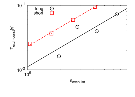
Figure 18: Time for the construction of the exchange list plotted against the average length of the list, for the case of $n_{p}=2048$ and $n\sim 2.7\times 10^{5},5.3\times 10^{5},1.1\times 10^{6},2.1\times 10^{6}$. Circles and squares indicate the results for long-range and short-range force, respectively. Solid and dashed curves are analytic models [equation (19)].

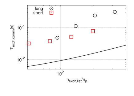
Figure 19: Time for the communication of the exchange list against the average length of the list per process, for the case of $n_{p}=2048$ and $n\sim 2.7\times 10^{5},5.3\times 10^{5},1.1\times 10^{6},2.1\times 10^{6}$. Circles and squares indicate the results for long-range and short-range force, respectively. The curve is predicted from equation (19).

In the following, we estimate $n_{\rm exch,list}$. If we consider a rather idealized case, in which all domains are cubes containing $n$ particles, the total length of the exchange lists for one domain can approximately be given by

$$n_{\rm exch,list}\sim\frac{14n^{2/3}}{\theta}+\frac{21\pi n^{1/3}}{\theta^{2}}+\frac{28\pi}{3\theta^{3}}{\rm log_{2}}\left\{\frac{\theta}{2.8}\left[\left(nn_{p}\right)^{1/3}-n^{1/3}\right]\right\},$$ (21)

for the case of long-range interactions and

$$n_{\rm exch,list}\sim\left(n^{1/3}-1+2\frac{r_{\rm cut}}{\left<r\right>}\right)^{3}-n,$$ (22)

for the case of short-range interactions, where $r_{\rm cut}$ is the average cutoff length and and $\left<r\right>$ is the average interparticle distance. In this section we set $r_{\rm cut}$ so that the number of particles in the neighbor sphere is to be 100. In other words, $r_{\rm cut}\sim 3\left<r\right>$.

In figure 20, we plot the list length for short and long interactions against the average number of particles. The rough estimate of equations (21) and (22) agree very well with the measurements.

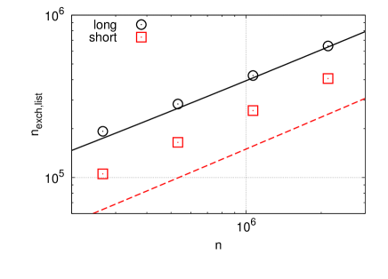
Figure 20: The average length of the exchange lists for long-range interaction (circles) and for short-range interaction (squares) as a function of $n$, in the case of $\theta=0.4$ and $n_{P}=2048$. Solid and dashed curves are predicted from equations (21) and (22), respectively.

5.5 Tree traverse and interaction calculation

The time for the force calculation is given by

$$T_{\rm icalc}=T_{\rm icalc,force}+T_{\rm icalc,const},$$ (23)

where $T_{\rm icalc,force}$ and $T_{\rm icalc,const}$ are the time for the force calculations for all particles and the tree traverses for all interaction lists, respectively.

$T_{\rm icalc,force}$ and $T_{\rm icalc,const}$ are expressed as

$$T_{\rm icalc,const} = \tau_{\rm icalc,const}nn_{\rm icalc,list}/n_{\rm grp},$$ (24)

$$T_{\rm icalc,force} = \tau_{\rm icalc,force}nn_{\rm icalc,list},$$ (25)

where $n_{\rm icalc,list}$ is the average length of the interaction list, $n_{\rm grp}$ is the number of $i$ particle groups for modified tree algorithms by Barnes (1990), $\tau_{\rm icalc,force}$ and $\tau_{\rm icalc,const}$ are the time for one force calculation and for constructing one interaction list. In figure 21, we plot the time for the construction of the interaction list as a function of $n_{\rm grp}$. On K computer, $\tau_{\rm icalc,const}$ are $3.72\times 10^{-8}$ second for the long-range force and $6.59\times 10^{-8}$ second for the short-range force.

Figure 21: Time for the construction of the interaction list for long-range force (circles) and short-range force (squares), for the case of $n\sim 5.3\times 10^{5}$ and $\theta=0.4$. Solid and dashed curves are the analytic models for long-rage and short range forces, respectively [equation (24)].

The length of the interaction list is given by

$$n_{\rm icalc,list}\sim n_{\rm grp}+\frac{14n_{\rm grp}^{2/3}}{\theta}+\frac{21\pi n_{\rm grp}^{1/3}}{\theta^{2}}+\frac{28\pi}{3\theta^{3}}{\rm log_{2}}\left[\frac{\theta}{2.8}\left\{\left(nn_{p}\right)^{1/3}-n_{\rm grp}^{1/3}\right\}\right]$$ (26)

for the case of long-range interactions and

$$n_{\rm icalc,list}\sim\left(n_{\rm grp}^{1/3}-1+2\frac{r_{\rm cut}}{\left<r\right>}\right)^{3},$$ (27)

for the case of short-range interactions.

In figure 22, we plot the length of the interactions lists for long-range force and short-range force. We can see that the length of the interaction lists can be fitted reasonably well.

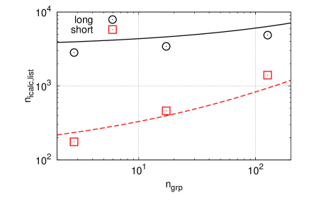
Figure 22: The average length of the interaction list for long-range force (circles) and short-range force (squares), for the case of $n\sim 5.3\times 10^{5}$ and $\theta=0.4$. Solid and dashed curves are analytic models for long-range [equation (26)] and short-range [equation (27)] forces.

In the following, we discuss the time for the force calculation. The time for the force calculation for one particle pair $\tau_{\rm icalc,force}$ has different values for different kinds of interactions. We plot $\tau_{\rm icalc,force}$ against $n_{\rm icalc,list}$ for various $n_{\rm grp}$ in figure 23. We can see that for larger $n_{\rm grp}$, $\tau_{\rm icalc,force}$ becomes smaller. However, from equation (26), large $n_{\rm grp}$ leads to large $n_{\rm icalc,list}$ and the number of interactions becomes larger. Thus there is an optimal $n_{\rm grp}$. In our disk-galaxy simulations in K computer, the optimal $n_{\rm grp}$ is a few hundreds, and dependence on $n_{\rm grp}$ is weak.

Figure 23: Time for the evaluation of one gravity force against $n_{\rm icalc,list}$ for various $n_{\rm grp}$.

5.6 Total time

Now we can predict the total time of the calculation using the above discussions. The total time per one timestep is given by

$$T_{\rm step} \sim T_{\rm dc,sort}/n_{\rm dc}+k_{\rm type}\left(T_{\rm exch,const}+T_{\rm exch,comm}\right)$$ (29)

$$+T_{\rm icalc,force}+T_{\rm icalc,const}$$

$$\sim \tau_{\rm dc,sort}n_{\rm smp}n_{p}^{2/3}/n_{\rm dc}$$

$$+k_{\rm type}\left(\tau_{\rm exch,const}n_{\rm exch,list}+\tau_{\rm alltoallv,startup}n_{p}+\tau_{\rm alltoallv,word}n_{\rm exch,list}b_{p}n_{p}^{1/3}\right)$$

$$+\tau_{\rm icalc,force}nn_{\rm icalc,list}$$

$$+\tau_{\rm icalc,const}nn_{\rm icalc,list}/n_{\rm grp}.$$

The time coefficients in equation (29) for K computer are summarized in table 2. In this section we use $n_{\rm dc}=1$.

Table 2: Time coefficients in equation (29) for K computer. $\tau_{\rm icalc,force}$ is the value for gravity.

$\tau_{\rm alltoallv,startup}$ [s]	$1.66\times 10^{-6}$
$\tau_{\rm alltoallv,word}$ [s/byte]	$1.11\times 10^{-10}$
$\tau_{\rm dc,sort}$ [s]	$2.67\times 10^{-7}$
$\tau_{\rm exch,const}$ [s]	$1.12\times 10^{-7}$
$\tau_{\rm icalc,const}$ [s]	$3.72\times 10^{-8}$
$\tau_{\rm icalc,force}$ [s]	$3.05\times 10^{-10}$

To see if the predicted time by equation (29) is reasonable, we compare the predicted time and the time obtained from the disk galaxy simulation with the total number of particles ($N$) of 550 million and $\theta=0.4$. In our simulations, we use up to the quadrupole moment. On the other hand, we assume the monopole moment only in equation (29). Thus we have to correct the time for the force calculation in equation (29). In our simulations, the cost of the force calculation of the quadrupole moment is two times higher than that of the monopole moment and about 75% of particles in the interactions list are superparticles. Thus the cost of the force calculation in the simulation is 75% higher than the prediction. We apply this correction to equation (29). In figure 24, we plot the breakdown of the predicted time with the correction and the obtained time from the disk galaxy simulations. We can see that our predicted times agree with the measurements very well.

Figure 24: Breakdown of the total time of the calculation per one timestep against $n_{p}$, for the case of $N=5.5\times 10^{8}$ , $n_{\rm smp}=500$, $\theta=0.4$ and $n_{\rm grp}=130$.

In the following, we analyze the performance of the gravitational many body simulations for various hypothetical computers. In figure 25, we plot the breakdown of the calculation time predicted using equation (29) for the cases of 1 billion and 10 million particles against $n_{p}$. For the case of 1 billion particles, we can see that the slope of $T_{\rm step}$ becomes shallower for $n_{p}\gtrsim 10000$ and increases for $n_{p}\gtrsim 30000$, because $T_{\rm dc,sort}$ dominates. Note that $T_{\rm exch,comm}$ also has the minimum value. The reason is as follows. For small $n_{p}$, $T_{\rm alltoallv,word}$ is dominant in $T_{\rm exch,comm}$ and it decrease as $n_{p}$ increases, because the length of $n_{\rm exch,list}$ becomes smaller. For large $n_{p}$, $T_{\rm alltoallv,startup}$ becomes dominant and it increases linearly. We can see the same tendency for the case of 10 million particles. However, the optimal $n_{p}$, at which $T_{\rm step}$ is the minimum, is smaller than that for 1 billion particles, because $T_{\rm dc,sort}$ is independent of $N$.

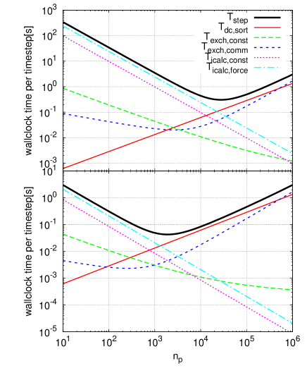
Figure 25: Breakdown of the total time of the calculation per one timestep against $n_{p}$, for the case of $N=10^{9}$ (top panel) and $=10^{7}$ (bottom panel), $n_{\rm smp}=500$, $\theta=0.4$ and $n_{\rm grp}=300$.

In figure 26, we plot the breakdown of the predicted calculation time for a hypothetical computer which has the floating-point operation performance ten times faster than that of K computer (hereafter X10). In other words, $\tau_{\rm alltoallv,startup}$ and $\tau_{\rm alltoallv,word}$ are the same as those of K computer, but $\tau_{\rm dc,sort}$, $\tau_{\rm exch,const}$, $\tau_{\rm icalc,const}$ and $\tau_{\rm icalc,force}$ are ten times smaller than those of K computer. We can see that the optimal $n_{p}$ is shifted to smaller $n_{p}$ for both cases of $N$ of 1 billion and 10 million, because $T_{\rm exch,comm}$ is unchanged. However, the shortest time per timestep is improved by about a factor of five. If the network performance is also improved by a factor of ten, we would get the same factor of ten improvement for the shortest time per timestep. In other words, by reducing the network performance by a factor of ten, we suffer only a factor of two degradation of the shortest time.

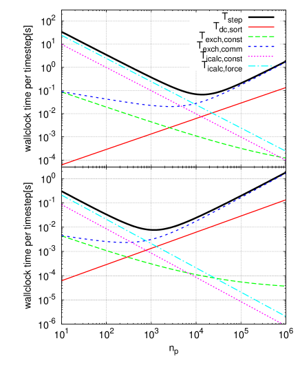
Figure 26: The same as figure 25, but for the floating-point operation performance ten times faster than K computer.

In figure 27, we plot predicted $T_{\rm step}$ for three hypothetical computers and K computer. Two of four computers are the same computer models we used above. Another is a computer with the floating-point operation performance hundred times faster than K computer (hereafter X100). The last one is a computer of which the performance of the force calculation is ten times faster than K computer (hereafter ACL). In other words, only $\tau_{\rm icalc,force}$ is ten times smaller than that of K computer. This computer is roughly mimicking a computer with an accelerator such as, GPU (Hamada et al., 2009b), GRAPE (Sugimoto et al., 1990; Makino et al., 2003) and PEZY-SC. Here we use the optimal $n_{\rm grp}$, at which $T_{\rm step}$ is minimum, for each computers. For the case of $N=10^{9}$, the optimal $n_{\rm grp}\sim 300$ for K computer and X10, $\sim 400$ for X100 and $\sim 1600$ for ACL. For the case of $N=10^{12}$, the optimal $n_{\rm grp}$ for K, X10, X100 is the same as those for $N=10^{9}$, but $\sim 1800$ for ACL. The optimal value of $n_{\rm grp}$ for ACL is larger than those of any other computers, because large $n_{\rm grp}$ reduces the cost of the construction of the interaction list.

From figure 27, we can see that for small $n_{p}$, X10 and X100 are ten and hundred times faster than K computer, respectively. However, for the case of $N=10^{9}$, $T_{\rm step}$ of the values of X10 and X100 increase for $n_{p}\gtrsim 15000$ and $\gtrsim 7000$, because the $T_{\rm exch,comm}$ becomes the bottleneck. ACL shows a similar performance to that of X10 up to optimal $n_{p}$, because the force calculation is dominant in the total calculation time. On the other hand, for large $n_{p}$, the performance of ACL is almost the same as that of K computer, because ACL has the same bottleneck as K computer has, which is the communication of the exchange list. On the other hand, for the case of $N=10^{12}$, $T_{\rm step}$ is scaled up to $n_{p}\sim 10^{5}$ for all computers. This is because for larger $N$ simulations, the costs of the force calculation and the construction of the interaction list are relatively higher than the communication of the exchange list. Thus the optimal $n_{p}$ is sifted to larger value if we use larger $N$.

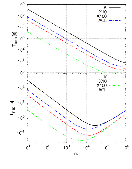
Figure 27: Predicted total calculation time for three hypothetical computers and K computer as a function of $n_{p}$, for the case of $n_{\rm smp}=500$, $\theta=0.4$. Top and bottom panels indicate the results of the case for $N=10^{12}$ and $N=10^{9}$, respectively.

From figures 25 and 26, we can see that for large $n_{p}$, performance will be limited by $T_{\rm dc,sort}$ and $T_{\rm exch,comm}$. Therefor, if we can reduce them further, we can improve the efficiency of the calculation with large $n_{p}$. It is possible to reduce the time for sort by applying the algorithm used in $x$ direction to $y$ direction as well or setting $n_{\rm dc}$ to more than unity. It is more difficult to reduce $T_{\rm exch,comm}$, since we are using system-provided MPI_Alltoallv.

6 Conclusion

In this paper, we present the basic idea, implementation, measured performance and performance model of FDPS, a framework for developing efficient parallel particle-based simulation codes. FDPS provides all of these necessary functions for the parallel execution of particle-based simulations. By using FDPS, researchers can easily develop their programs which run on large-scale parallel supercomputers. For example, a simple gravitational $N$-body program can be written in around 120 lines.

We implemented three astrophysical applications using FDPS and measured their performances. All applications showed good performance and scalability. In the case of the disk galaxy simulation, the achieved efficiency is around 50% of the theoretical peak, for the cosmological simulation 7%, and for the giant impact simulation 40%.

We constructed the performance model of FDPS and analyzed the performance of applications using FDPS. We found that the performance for small number of particles would be limited by the time for the calculation necessary for the domain decomposition and communication necessary for the interaction calculation.

We thank M. Fujii for providing initial conditions of spiral simulations, T. Ishiyama for providing his Particle Mesh code, K. Yoshikawa for providing his TreePM code and Y. Maruyama for being the first user of FDPS. We are grateful to M. Tsubouchi for her help in managing the FDPS development team. This research used computational resources of the K computer provided by the RIKEN Advanced Institute for Computational Science through the HPCI System Research project (Project ID:ra000008). Part of the research covered in this paper research was funded by MEXT’s program for the Development and Improvement for the Next Generation Ultra High-Speed Computer System, under its Subsidies for Operating the Specific Advanced Large Research Facilities. Numerical computations were in part carried out on Cray XC30 at Center for Computational Astrophysics, National Astronomical Observatory of Japan.

References

- Abrahama et al. (2014) Abrahama, M. J., Murtolad, T., Schulzb, R., Palla, S., Smithb, J., Hessa, B. & Lindahl., E. 2015, SoftwareX, 1, 19
- Asphaug & Reufer (2014) Asphaug, E. & Reufer, A. 2014, Nature Geoscience, 7, 564
- Bagla (2002) Bagla, J. S. 2002, JApA, 23, 185
- Balsara (1995) Balsara, D. S. 1995, JCoPh, 121, 357
- Barnes & Hut (1986) Barnes, J. and Hut, P. 1986, Nature, 324, 446
- Barnes (1990) Barnes, J. 1990, JCoPh, 87, 161
- Bédorf et al. (2012) Bédorf, J., Gaburov, E. & Portegies Zwart, S. 2012, JCoPh, 231, 2825
- Bédorf et al. (2014) Bédorf, J., Gaburov, E., Fujii, M., Nitadori, K., Ishiyama, T., & Portegies Zwart, S. 2014, Proceedings of the International Conference for High Performance Computing, Networking, Storage and Analysis, IEEE Press, 54
- Benz et al. (1986) Benz, W., Slattery, W. L. & Cameron, A. G. W. 1986, Icarus, 66, 515
- Blackston & Suel (1997) Blackston, D., & Suel, T. 1997, Proc. of the ACM/IEEE Conf. on Supercomputing, ACM, 1
- Bode et al. (2000) Bode, P., Ostriker, J. P. & Xu, G. 2000, ApJS, 128, 561
- Brooks et al. (2009) Brooks, B., et al. 2009, J. Comp. Chem. 30, 1545
- Cameron & Ward (1976) Cameron, A. G. W. & Ward, W. R. 1976, Lunar and Planetary Science Conference, 7, 120
- Canup et al. (2013) Canup, R. M., Barr, A. C. & Crawford, D. A. 2013, Icarus, 222, 200
- Case et al. (2015) Case, D. A., et al. 2015, AMBER 2015, (San Francisco:University of California)
- Dehnen & Aly (2012) Dehnen, W. & Aly, H. 2012, MNRAS, 425, 1068
- Dehnen (2000) Dehnen, W. 2000, ApJ, 536, L39
- Dubinski (1996) Dubinski, J. 1996, NewA, 1, 133,
- Dubinski et al. (2004) Dubinski, J., Kim, J., Park, C. & Humble, R. 2004, NewA, 9, 111
- Fujii et al. (2011) Fujii, M. S., Baba, J., Saitoh, T. R., Makino, J., Kokubo, E., & Wada, K. 2011, ApJ, 730, 109
- Gaburov et al. (2009) Gaburov, E., Harfst, S. & Portegies Zwart, S. 2009, NewA, 14, 630
- Goodale et al. (2003) Goodale, T., Allen, G., Lanfermann, G., Massó, J., Radke, T., Seidel, E. & Shalf, J. 2003, 5th International Conference, Lecture Notes in Computer Science, 2565
- Hamada et al. (2009a) Hamada, T., Narumi, T., Yokota, R., Yasuoka, K., Nitadori, K., & Taiji, M. 2009, Proceedings of the Conference on High Performance Computing Networking, Storage and Analysis, 62, 1
- Hamada et al. (2009b) Hamada, T., Nitadori, K., Benkrid, K., Ohno, Y., Morimoto, G., Masada, T., Shibata, Y., Oguri, K. & Taiji, M. 2009, Computer Science-Research and Development, 24, 21
- Hamada & Nitadori (2010) Hamada, T., & Nitadori, K. 2010, Proceedings of the ACM/IEEE International Conference for High Performance Computing, Networking, Storage and Analysis, IEEE Computer Society, 1
- Hartmann & Davis (1975) Hartmann, W. K. & Davis, D. R. 1975, Icarus, 24, 504
- Hernquist (1990) Hernquist, L. 1990, ApJ, 356, 359
- Hockney & Eastwood (1988) Hockney, R. W. & Eastwood, J. W. 1988, Computer Simulation Using Particles, CRC Press
- Ishiyama et al. (2009) Ishiyama, T., Fukushige, T. & Makino, J. 2009, PASJ, 61, 1319
- Ishiyama et al. (2012) Ishiyama, T., Nitadori, K., & Makino, J. 2012, Proceedings of the International Conference on High Performance Computing, Networking, Storage and Analysis, 5, 1
- Iwasawa et al. (2015) Iwasawa, M., Tanikawa, A., Hosono, N., Nitadori, K., Muranushi, T. & Makino, J. 2015, WOLFHPC ’15, 1, 1
- Navarro et al. (1996) Navarro, J. F., Frenk, C. S. & White, S. D. M. 1996, ApJ, 462, 563
- Nitadori et al. (2006) Nitadori, K., Makino, J. & Hut, P. 2006, NewA, 12, 169
- Makino (1991) Makino, J. 1991, PASJ, 43, 859
- Makino et al. (2003) Makino, J., Fukushige, T., Koga, M., & Namura, K. 2003, PASJ, 55, 1163
- Makino (2004) Makino, J. 2004, PASJ, 56, 521
- Monaghan (1992) Monaghan, J. J. 1992, ARA&A, 30, 543
- Monaghan (1997) Monaghan, J. J. 1997, J. Comp. Phys., 136, 298
- Murotani et al. (2014) Murotani, K., et al. 2014, Journal of Advanced Simulation in Science and Engineering, 1, 16
- Phillips et al. (2005) Phillips, J., et al. 2005 J. Comp. Chem., 26, 1781
- Plimpton (1995) Plimpton, S. 1995, J. Comp. Phys., 117, 1
- Rosswog (2009) Rosswog, S. 2009, NewAR, 53, 78
- Salmon & Warren (1994) Salmon, J. K. & Warren, M. S. 1994, 111, 136,
- Schuessler & Schmitt (1981) Schuessler, I. & Schmitt, D. 1981, A&A, 97, 3735
- Shaw et al. (2014) Shaw, D. E., et al. 2014, Proceedings of the International Conference on High Performance Computing, Networking, Storage and Analysis, 41
- Springel (2005) Springel, V. 2005, MNRAS, 364, 1105
- Springel et al. (2005) Springel, V., et al., 2005, Nature, 435, 629
- Springel (2010) Springel, V. 2010, ARA&A, 48, 391
- Sugimoto et al. (1990) Sugimoto, D., et al. 1990, Nature, 345, 33
- Tanikawa et al. (2012) Tanikawa, A., Yoshikawa, K., Okamoto, T. & Nitadori, K. 2012, NewA, 17, 82
- Tanikawa et al. (2013) Tanikawa, A., Yoshikawa, K., Nitadori, K. & Okamoto, T. 2013, NewA, 19, 74
- Teodoro et al. (2014) Teodoro, L. F. A., Warren, M. S., Fryer, C., Eke, V. & Zahnle,,K. 2014, Lunar and Planetary Science Conference, 45, 2703
- Wadsley et al. (2004) Wadsley, J. W., Stadel, J. & Quinn, T. 2004, NewA, 9, 137
- Warren & Salmon (1995) Warren, M. S., & Salmon, J. K. 1995, Computer Physics Communications, 87, 266
- (55) M. S. Warren, J. K. Salmon, D. J. Becker, M. P. Goda, T. L. Sterling, & W. Winckelmans, 1997, Proceedings of the International Conference on High Performance Computing, Networking, Storage and Analysis, 61
- Widrow & Dubinski (2005) Widrow, L. M. & Dubinski, J. 2005, ApJ, 631, 838
- Xu (1995) Xu, G. 1995, ApJS, 98, 355
- Yamada et al. (2015) Yamada, T., Mitsume, N., Yoshimura, S. & Murotani, K. 2015, COUPLED PROBLEMS 2015
- Yoshikawa & Fukushige (2005) Yoshikawa, K. & Fukushige, T. 2005, PASJ, 57, 849