Star-type oscillatory networks with generic Kuramoto-type coupling: a model for “Japanese drums synchrony”

Abstract

We analyze star-type networks of phase oscillators by virtue of two methods. For identical oscillators we adopt the Watanabe-Strogatz approach, that gives full analytical description of states, rotating with constant frequency. For nonidentical oscillators, such states can be obtained by virtue of the self-consistent approach in a parametric form. In this case stability analysis cannot be performed, however with the help of direct numerical simulations we show which solutions are stable and which not. We consider this system as a model for a drum orchestra, where we assume that the drummers follow the signal of the leader without listening to each other and the coupling parameters are determined by a geometrical organization of the orchestra.

In the various studies of synchronization of globally coupled ensembles of oscillators, usually, it is assumed that global coupling is produced by mean fields that act directly on each oscillator. However, in many natural systems (for example arrays of Josephson junctions), the global field is produced by a dynamical unit. In this paper we consider the case when this unit is a limit cycle oscillator, that can be described by a phase equation, similar to that for the other oscillators in the ensemble. Such configuration of oscillators is often called star-type network. In the first part of the paper we study the case of identical oscillators by virtue of the Watanabe-Strogatz approach that gives full analytical analysis of steady solutions. In the second part we examine inhomogeneous case, when the parameters of the coupling between each oscillator and the central element are different. Such network can be considered as a model for Japanese drums orchestra, consisting of a battery of drummers and a leader, where the drummers only follow the signal from the leader. With the help of the self-consistent approach we find solutions when the global field rotates uniformly. These solutions are obtained semi-analytically in a parametric form. In this work we analyze the case when the distribution of the parameters is determined by the geometric organization of the oscillators. However, this approach can be applied for an arbitrary distribution of the parameters.

I Introduction

Studies of synchronization in populations of coupled oscillators attract high interest. First, there are many experimental realizations of this effect, ranging from physical systems (lasers, Josephson junctions, spin-torque oscillators) to biology (fireflies, genetically manipulated circuits) and social activity of humans and animals (hand clapping, pedestrian footwalk on a bridge, egg-laying in bird colonies), see reviews Acebrón et al. (2005); Pikovsky and Rosenblum (2015) for these and other examples. Second, from the theoretical viewpoint, synchronization represents an example of a nonequilibrium phase transition, and the challenging task is to describe it as complete as possible in terms of suitable order parameters (global variables). In the simplest setup of weakly coupled oscillators interacting via mean fields, the Kuramoto model of globally coupled phase oscillators Kuramoto (1975, 1984) and its generalizations are widely used. Here three main approaches have been developed. The original theory by Kuramoto is based on solving the self-consistent equations for the mean fields. In a particular case of sine-coupled identical phase oscillators, the Watanabe-Strogatz theory Watanabe and Strogatz (1993, 1994) allows one to derive a closed set of equations for the order parameters. For non-identical sine-coupled oscillators, an important class of dynamical equations for the order parameters is obtained via the Ott-Antonsen ansatz Ott and Antonsen (2008).

Typically, coupling in the ensemble is considered as a force directly produced by mean fields (either in a linear or nonlinear way). However, a more general setup includes equations for global variables, driven by mean fields and acting on the oscillators. For example, for Josephson junctions and spin-torque oscillators, the coupling is due to a common load Wiesenfeld et al. (1996); Pikovsky (2013), which may include inertial elements (like capacitors and inductances) and therefore one gets an additional system of equations (linear or nonlinear Pikovsky and Rosenblum (2009), depending on the properties of the load) for global variables and mean fields. A special situation appears when the mediator of the coupling is not a linear damped oscillator (like an LCR load for Josephson junctions), but an active, limit cycle oscillator. In this case the latter may be described by a phase equation similar to that describing one oscillator in the population. Such an ensemble, where “peripheral” oscillators are coupled through one “central” oscillator, corresponds to a star-type network of interactions Kazanovich and Borisyuk (2003); Burylko et al. (2012); Kazanovich et al. (2013).

One can make an analogy of such a network and a Japanese drums orchestra. Such an orchestra consists of a battery of drummers and a leader, who sets the rhythm of the music. In our model the battery corresponds to an ensemble of oscillators coupled to a leader, who also is an oscillator. Although in practice each drummer represents a pulse oscillator (like a spiking neuron), we adopt here the phase description like in the Kuramoto model. One should have in mind that we do not aim in this paper to describe a real Japanese drum orchestra operation, but rather use this the analogy to make the interpretation of the results demonstrative.

In this paper we apply the methods for description of global dynamics to such star-type networks with generic coupling (see Vlasov et al. (2014) for generic algebraic coupling), where interactions of oscillators with the central element (i.e. their coupling constants and phase shifts) are in general different, and are described by some joint distribution function. We should stress that “generic” in this context means not including coupling functions of arbitrary shape, but rather allowing for arbitrary distribution of parameters (amplitudes and phase shifts) of the Kuramoto-type sin-coupling terms. In the first part of the paper we present full analytical analysis of the homogenous case (the intrinsic frequencies of all oscillators and the coupling constants are the same for all oscillators) in the framework of the Watanabe-Strogatz (WS) approach (see Vlasov, Zou and Pereira (2015) for the particular case of coupling coefficients). Due to the fact that the WS method leads to a low-dimensional system of equations that describes dynamics of a homogenous ensemble of any size, it is possible to analyze also stability of obtained solutions. We present solutions together with their stability for different sets of parameters. In the second part we perform the analysis of an inhomogeneous system with the help of the self-consistent approach. After derivation of general equations valid for an arbitrary distribution of coupling parameters, we consider a particular example inspired by the analogy to the drum orchestra: we assume that the phase shifts and coupling strengths follow from a geometric configuration of the “battery” and from the position of the “conductor”. In this case, the stability analysis could not be performed, but we compare obtained self-consistent solutions with the results of direct numerical simulations.

II The model

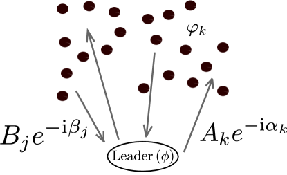
Figure 1: Configuration of the network, coupled through a leader.

We consider a system of phase oscillators with a leader-type coupling. Such a network structure (Fig. 1) is often called star network, that is the simplest small-world network. In our setup, in the most general case each phase oscillator $\varphi_{k}$ has its own frequency $\omega_{k}$ and is forced by the leader oscillator (phase $\phi$) with its own coupling strength $A_{k}$ and phase shift $\alpha_{k}$. At the same time, the leader $\phi$ has its own frequency $\omega_{0}$ and is forced by every other oscillator $\varphi_{j}$ with coupling coefficient $B_{j}$ and phase shift $\beta_{j}$. The dynamical equations thus read

$$\begin{split}\dot{\varphi_{k}}&=\omega_{k}+A_{k}\sin(\phi-\varphi_{k}-\alpha_{k}),\quad k=1\ldots N,\\ \dot{\phi}&=\omega_{0}+{1\over N}\sum_{j=1}^{N}B_{j}\sin(\varphi_{j}-\beta_{j}-\phi).\end{split}$$ (1)

The system (1) can be rewritten in terms of the mean field

$$\begin{split}\dot{\varphi_{k}}&=\omega_{k}+{\rm Im}(A_{k}e^{\text{i}(\phi-\varphi_{k}-\alpha_{k})}),\\ \dot{\phi}&=\omega_{0}+{\rm Im}(\tilde{G}(t)e^{-\text{i}\phi}),\\ \tilde{G}(t)&={1\over N}\sum_{j=1}^{N}B_{j}e^{\text{i}(\varphi_{j}-\beta_{j})}.\end{split}$$ (2)

It is convenient to perform a variable transformation to the phase differences $\Delta\varphi_{k}$ between the oscillators $\varphi_{k}$ and the leader $\phi$, taking also into account the phase shift $\alpha_{k}$:

$$\Delta\varphi_{k}=\varphi_{k}-\phi+\alpha_{k}.$$ (3)

Then, the equations for $\Delta\varphi_{k}$ and $\phi$ are

$$\begin{split}\frac{d\Delta\varphi_{k}}{dt}&=-\frac{d\phi}{dt}+\omega_{k}+{\rm Im}(A_{k}e^{-\text{i}\Delta\varphi_{k}}),\\ \frac{d\phi}{dt}&=\omega_{0}+{\rm Im}(G(t)),\\ G(t)&={1\over N}\sum_{j=1}^{N}B_{j}e^{\text{i}(\Delta\varphi_{j}-\alpha_{j}-\beta_{j})}.\end{split}$$ (4)

The expression for the leader dynamics can be directly inserted into the equations for $\Delta\varphi_{k}$, and thus we obtain the effective mean-field-coupled closed system

$$\begin{split}\frac{d\Delta\varphi_{k}}{dt}&=\omega_{k}-\omega_{0}-{\rm Im}(G(t))+{\rm Im}(A_{k}e^{-\text{i}\Delta\varphi_{k}}),\\ G(t)&={1\over N}\sum_{j=1}^{N}B_{j}e^{\text{i}(\Delta\varphi_{j}-\alpha_{j}-\beta_{j})}.\end{split}$$ (5)

The system (5) is equivalent to the phase model (1) for the leader-type (star) networks. This model in the form (5) is similar to the models of Josephson junction arrays with the star-like topology, which have been considered previously in Tsang et al. (1991); Golomb et al. (1992); Swift et al. (1992). Analytical analysis similar to that described below has been performed for Josephson junction arrays in Vlasov and Pikovsky (2013) . In Kazanovich and Borisyuk (2003) the model (1) for the systems with center element (leader coupling) has been considered in the case of identical coupling parameters and the distribution of natural frequencies of the leaf oscillators.

In this work we are going to study the cases of identical and nonidentical oscillators separately. Below we present the analytical analysis for these two cases together with numerical simulations for a particular example of nonidentical oscillators. In case of identical oscillators, we apply the Watanabe-Strogatz approach. For the analysis of the case of nonidentical units the self-consistent approach is used.

III Identical oscillators

If all the parameters $\omega_{k}$, $A_{k}$, $B_{j}$, $\beta_{j}$ and $\alpha_{j}$ are identical, then the form of the phase equation (which is a particular case of Eq. (5))

$$\begin{split}\frac{d\Delta\varphi_{k}}{dt}&=\omega-\omega_{0}-{\rm Im}\left(G(t)\right)+{\rm Im}(Ae^{-\text{i}\Delta\varphi_{k}}),\\ G(t)&=Be^{-\text{i}(\alpha+\beta)}{1\over N}\sum_{j=1}^{N}e^{\text{i}\Delta\varphi_{j}}.\end{split}$$ (6)

allows us to use the WS ansatz Watanabe and Strogatz (1993, 1994), which is applicable to any system of identical phase equations of the general form

$$\dot{\varphi_{k}}=f(t)+{\rm Im}\left(F(t)e^{-\text{i}\varphi_{k}}\right),$$ (7)

with arbitrary real function $f(t)$ and complex function $F(t)$. It consists of the idea that after WS variable transformation (8), the dynamics of the ensemble (7) is characterized by one global complex variable $z=z(t)$ and one real global variable $\Psi=\Psi(t)$, and $N$ constants of motion $\psi_{k}$ (of which only $N-3$ are independent). We use the formulation of the WS theory presented in Pikovsky and Rosenblum (2011). WS transformation (8) is essentially the Möbius transformation Marvel et al. (2009) in the form

$$e^{\text{i}\varphi_{k}}=\frac{z+e^{\text{i}(\psi_{k}+\Psi)}}{1+z^{*}e^{\text{i}(\psi_{k}+\Psi)}},$$ (8)

with additional constraints $\sum_{i}e^{\text{i}\psi_{i}}=\sum_{i}\cos 2\psi_{i}=0$. Then the global variables’ dynamics is determined by

$$\begin{split}\dot{z}&=\text{i}f(t)z+{F(t)\over 2}-{F^{*}(t)\over 2}z^{2},\\ \dot{\Psi}&=f(t)+{\rm Im}(z^{*}F(t)).\end{split}$$ (9)

Comparing the system (6) with (7) we see that in our case $f(t)=\omega-\omega_{0}-{\rm Im}\left(G(t)\right)$ and $F(t)=A$. The next step is to express the function $G(t)$, that is essentially the order parameter multiplied by a complex number, in the new global variables. In general, such an expression is rather complex (see Pikovsky and Rosenblum (2011) for details), but in the thermodynamic limit $N\to\infty$ and for a uniform distribution of constants of motion $\psi$ (the index has been dropped because constants now have a continuous distribution) the order parameter is equal to $z$ (see Appendix A). The constants $\psi$, as well as the WS variables $z(0)$ and $\Psi(0)$, are determined by initial conditions for the original phases $\Delta\varphi(0)$. In fact, any distribution of the constants is possible, and for each such distribution the dynamics will be different. However, as has been argued in Ref. Pikovsky and Rosenblum (2009), in presence of small perturbations, initially non-uniform constants tend toward the uniform distribution, which also the one appearing in the Ott-Antonsen ansatz Ott and Antonsen (2008). Due to these special relevance of the uniform distribution of the constants $\psi$, we consider only this case below.

In this case, it follows from (9) that $\Psi$ does not enter the equation for $z$, so we obtain a closed equation for $z$ that describes system (6):

$$\dot{z}=\text{i}\left(\Delta\omega-B\,{\rm Im}(ze^{-\text{i}\delta})\right)z-A\frac{z^{2}-1}{2},$$ (10)

where $\Delta\omega=\omega-\omega_{0}$ and $\delta=\alpha+\beta$.

For a further analysis, it is appropriate to represent the complex variable $z=\rho e^{\text{i}\Delta\Phi}$ in polar form. Thus

$$\begin{split}\frac{d\rho}{dt}&=A\frac{1-\rho^{2}}{2}\cos\Delta\Phi,\\ \frac{d\Delta\Phi}{dt}&=\Delta\omega+B(\sin\delta)\rho\cos\Delta\Phi-\frac{A+(A+2B\cos\delta)\rho^{2}}{2\rho}\sin\Delta\Phi.\end{split}$$ (11)

Note that Eqs. (11) are invariant under the following transformation of variables and parameters: $\Delta\Phi\to-\Delta\Phi$, $\Delta\omega\to-\Delta\omega$ and $\delta\to-\delta$.

III.1 Steady states

We start the analysis of (11) with finding its steady states. From the first equation in (11) it follows that there are two types of steady states with $\dot{\rho}=0$: synchronous with $\rho=1$ and asynchronous with $\cos\Delta\Phi=0$. The synchronous steady state gives

$$\begin{split}\rho&=1,\\ \frac{d\Delta\Phi}{dt}&=\Delta\omega-\sqrt{A^{2}+B^{2}+2AB\cos\delta\,}\sin\left(\Delta\Phi+\arcsin\frac{A+B\cos\delta}{\sqrt{A^{2}+B^{2}+2AB\cos\delta\,}}-\frac{\pi}{2}\right).\end{split}$$ (12)

From (12) it follows that the steady solution $\frac{d\Delta\Phi}{dt}=0$ exists only if $|\Delta\omega|\leq\sqrt{A^{2}+B^{2}+2AB\cos\delta\,}$.

By rescaling time, we can reduce the number of parameters. Eq. (12) suggests that the mostly convenient rescaling is

$$t^{\prime}=t\sqrt{A^{2}+B^{2}+2AB\cos\delta\,}.$$ (13)

This rescaling is quite general except for two special cases when $\cos\delta=-1$ and $B=A$ (see Appendix B) or $A=B=0$, the latter case is just one of uniformly rotating uncoupled phase oscillators that does not present any interest. So in the new parametrization Eqs. (12) have the form

$$\begin{split}\rho&=1,\\ \frac{d\Delta\Phi}{dt}&=\Delta x-\sin\left(\Delta\Phi+\xi-\frac{\pi}{2}\right),\end{split}$$ (14)

where

$$\Delta x=\frac{\Delta\omega}{\sqrt{A^{2}+B^{2}+2AB\cos\delta\,}\,}\ \ \ \text{and}\ \ \ \sin\xi=\frac{A+B\cos\delta}{\sqrt{A^{2}+B^{2}+2AB\cos\delta\,}\,}.$$ (15)

Thus the steady solutions of Eq. (14) have the following phases

$${\Delta\Phi_{s}}_{1}=\frac{\pi}{2}+\arcsin\Delta x-\xi,\ \ \ {\Delta\Phi_{s}}_{2}=-\frac{\pi}{2}-\arcsin\Delta x-\xi.$$ (16)

In the new parametrization Eqs. (11) have the form

$$\begin{split}\frac{d\rho}{dt}&=g\frac{1-\rho^{2}}{2}\cos\Delta\Phi,\\ \frac{d\Delta\Phi}{dt}&=\Delta x+(\cos\xi)\rho\cos\Delta\Phi-\frac{g+(2\sin\xi-g)\rho^{2}}{2\rho}\sin\Delta\Phi,\end{split}$$ (17)

where $g=\frac{A}{\sqrt{A^{2}+B^{2}+2AB\cos\delta\,}\,}\geq 0$. Note that similar to Eqs. (11), Eqs. (17) are invariant to the following transformation of variables and parameters $\Delta\Phi\to-\Delta\Phi$, $\Delta x\to-\Delta x$ and $\cos\xi\to-\cos\xi$. Due to this symmetry we can consider only the case when $\cos\xi\geq 0$.

The asynchronous steady states can be found from

$$\begin{split}\Delta\Phi&=\pm\,\pi/2,\\ 0&=\Delta x\mp\frac{g+(2\sin\xi-g)\rho^{2}}{2\rho}.\end{split}$$ (18)

Eq (18) gives two asynchronous steady solutions:

$${z_{a}}_{1,2}=\text{i}\frac{\Delta x\pm\sqrt{\Delta x^{2}-g(2\sin\xi-g)}}{2\sin\xi-g}.$$ (19)

It is convenient to rewrite Eq. (19) as

$${z_{a}}_{1,2}=\text{sign}(\Delta x)\,\text{i}\frac{|\Delta x|\pm\sqrt{\Delta x^{2}-g(2\sin\xi-g)}}{2\sin\xi-g}.$$ (20)

Note, that here the cases split, depending on the value of $(2\sin\xi-g)$. If $|2\sin\xi-g|>g$, then, because $\rho=|z|\leq 1$, the solution ${z_{a}}_{1}$ exists only if $|\Delta x|\leq|\sin\xi|$. If $|2\sin\xi-g|\leq g$, then, also because $\rho=|z|\leq 1$, the solution ${z_{a}}_{2}$ exists only if $|\Delta x|\geq\sin\xi$. If $2\sin\xi-g=0$, then the asynchronous steady solutions are

$${z_{a}}_{1,2}=\pm\,\text{sign}(\Delta x)\,\text{i}\frac{g}{2|\Delta x|},$$ (21)

but the condition on $|\Delta x|\geq\sin\xi=g/2$ is still the same.

Note that the expression $2\sin\xi-g$ is equal to $\frac{A+2B\cos\delta}{\sqrt{A^{2}+B^{2}+2AB\cos\delta\,}\,}$; if $\cos\delta\geq 0$ this expression is always positive, so that $g<1$ and $\sin\xi>g$. If $\cos\delta<0$, then the sign of this expression depends on the sign of $A+2B\cos\delta$, but $\sin\xi<g$.

III.2 Stability analysis

In order to analyze stability of the asynchronous steady solutions (20) we linearize the system around corresponding fixed point. The linearized system reads

$$\begin{split}\dot{a}_{1,2}&=\text{sign}(\Delta x)\left(-(\cos\xi)\,\frac{|\Delta x|\pm\sqrt{\Delta x^{2}-g(2\sin\xi-g)}}{2\sin\xi-g}\,a_{1,2}\pm\,\sqrt{\Delta x^{2}-g(2\sin\xi-g)}\,b_{1,2}\right),\\ \dot{b}_{1,2}&=\text{sign}(\Delta x)\left(|\Delta x|-(\sin\xi)\,\frac{|\Delta x|\pm\sqrt{\Delta x^{2}-g(2\sin\xi-g)}\,}{2\sin\xi-g}\right)a_{1,2},\end{split}$$ (22)

where $a_{1,2}$ and $b_{1,2}$ are real and imaginary parts of the perturbation, respectively. Although it is difficult to find explicit expressions for the eigenvalues of the linear system (22), compared to a straightforward calculation of eigenvalues for the synchronous fixed points below, it is possible to find regions of parameters where they are positive or negative, what is sufficient for determining stability of asynchronous solutions (see Appendix C for detailed description of stability properties of the asynchronous states).

There is one truly remarkable case when $\cos\xi=0$ or $\sin\delta=0$. In this case, eigenvalues of the linear system (22) for ${z_{a}}_{2}$ are purely imaginary, what opens a possibility for the fixed point ${z_{a}}_{2}$ to be neutrally stable (see subsection III.3 for details).

For two synchronous fixed points (16): ${z_{s}}_{1}=e^{\text{i}{\Delta\Phi_{s}}_{1}}$ and ${z_{s}}_{2}=e^{\text{i}{\Delta\Phi_{s}}_{2}}$, the corresponding linearized system reads

$$\begin{split}\dot{a}_{1,2}=&\Biggl{[}\mp\sqrt{1-\Delta x^{2}}+(\sin\xi-g)(-\Delta x\cos\xi\pm\sqrt{1-\Delta x^{2}}\sin\xi)\Biggr{]}a_{1,2}+\\ &+\Biggl{[}(\sin\xi-g)(\pm\sqrt{1-\Delta x^{2}}\cos\xi+\Delta x\sin\xi)\Biggr{]}b_{1,2},\\ \dot{b}_{1,2}=&\Biggl{[}\cos\xi(-\Delta x\cos\xi\pm\sqrt{1-\Delta x^{2}}\sin\xi)\Biggr{]}a_{1,2}+\\ &+\Biggl{[}-\sin\xi(-\Delta x\cos\xi\pm\sqrt{1-\Delta x^{2}}\sin\xi)\Biggr{]}b_{1,2},\end{split}$$ (23)

with the same meaning of linear perturbations $a_{1,2}$, $b_{1,2}$. Linear system (23) has two eigenvalues:

$$\begin{split}{\lambda_{s}}_{1,2}^{1}&=g(\Delta x\cos\xi\mp\sqrt{1-\Delta x^{2}}\sin\xi),\\ {\lambda_{s}}_{1,2}^{2}&=\mp\sqrt{1-\Delta x^{2}}.\end{split}$$ (24)

Their signs depend on the values of the parameters. We will outline all possible steady solutions together with their stability below (see Appendix C for a full description of stability properties of the steady solutions).

III.3 Reversible case when condition $\sin\delta=0$ holds

As has been shown by the stability analysis above, when $\sin\delta=0$, the steady state ${z_{a}}_{2}$ is neutrally stable for any $\Delta x$. The neutral stability can be proved by the fact that when $\sin\delta=0$ (and, as a consequence, $\cos\xi=0$), Eq. (10) is invariant to the transformation ${\rm Im}(z)\to{\rm Im}(z)$, ${\rm Re}(z)\to-{\rm Re}(z)$, when the time direction is also changed: $t\to-t$. This transformation, which leaves the imaginary axis invariant, is an involution. Thus, the dynamics is reversible Roberts and Quispel (1992): any trajectory that crosses ${\rm Im}(z)$ axes twice is a neutrally stable closed curve (Fig. 2). This set of quasi-Hamiltonian trajectories (surrounded by a homoclinic one) coexists with an attractor and a repeller, which are symmetric to each other (for other examples of coexistence of conservative and dissipative dynamics in reversible systems see, e.g., Politi et al. (1986)). In direct numerical simulations, one observes, depending on initial conditions, either a synchronous state, or oscillations of the order parameter $z$.

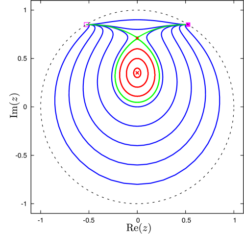
Figure 2: The phase portrait for the reversible order parameter dynamics (case $\sin\xi=1$, $\Delta x=0.85$, and $g=0.4$). Trajectories connecting the unstable synchronous fixed point (denoted as the empty square) and the stable one (filled square) are shown in blue. Trajectories oscillating around neutrally stable fixed point (x-cross) are shown in red. Stable and unstable manifolds of the saddle (denoted as the plus marker) are shown in green.

III.4 Synchronization scenarios

There are three main regions of parameters with three different transitions from asynchronous steady solution to synchronous one.

We present the diagram of different states in the parameter plane $(\delta,\Delta x)$ in the Fig. 3. There are three main domains: the domain, where the synchronous solution (illustrated in Fig. 4(a)) is stable; the domain where the asynchronous solution (illustrated in Fig. 4(b)) is stable; and the domain of bistability. As parameters $\delta$ and $\Delta x$ describe two main properties of the star-type coupling, namely the phase shift in the coupling and the frequency mismatch between the central and peripheral elements, correspondingly, the interpretation of these domains is straightforward. Phase shifts close to zero, as well as small frequency mismatches facilitate synchrony; bistability is observed when the mismatch is relatively large while the phase shift $\delta$ is close to the optimal one for synchronization (zero).

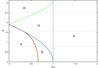
Figure 3: Different regimes in the parameter plane $(\delta,\Delta x)$ for $A=1$ and $B=3$. The area, where the synchronous steady solution is stable, is denoted with $s$, the areas, where asynchronous steady solution is stable, are denoted with $a$, the area of the hysteresis is denoted with $h$. Solid red line is stability line of the asynchronous state, solid blue line is stability line of the synchronous state. Dashed green line denotes the area of existence of unstable asynchronous solution and dashed blue line - the area of existence of unstable synchronous solution. Horizontal dashed gray lines are cuts of the diagram illustrated in Fig 5 ((a) corresponds to the bottom line, (b) - to the middle line and (c) - to the top line).

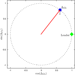
(a) (b)

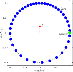
Figure 4: Snapshots of the oscillators for synchronous ((a) $\Delta x=0.3$) and asynchronous ((b) $\Delta x=0.7$) cases. The parameters are the same as for the Fig. 5(a).

We show the transitions in dependence on the relative frequency mismatch $\Delta x$ between the oscillator’s natural frequency and the frequency of the leader. Stability of the solutions depends on the sign of the frequency mismatch $\Delta x$. A detailed description of the solutions we present in Appendix C.

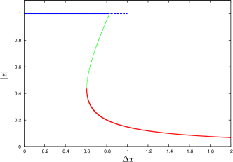
(a) (b)

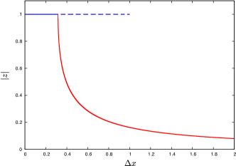
(c)

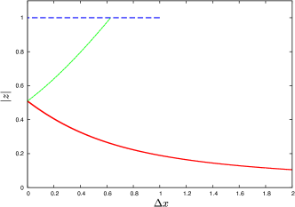
Figure 5: The dependence of the order parameter $|z|$ on the relative frequency mismatch $\Delta x$, for the case $\sin\xi>g\geq 0$ (a), for the case $g\geq\sin\xi\geq 0$ (b) and for the case $\sin\xi<0$ (c). The red curve denotes stable asynchronous steady solution, the green curve denotes unstable asynchronous steady solution and solid blue line denotes synchronous steady solution, while dashed blue line denotes unstable synchronous steady solution.

In the first case (Fig. 5(a)) there is a hysteretic synchronization transition. If $\Delta x>0$, there is a stable asynchronous steady solution that exists for large absolute values of $|\Delta x|$, and a stable synchronous steady solution that exists for small $|\Delta x|$. These solutions coexist for a bounded region of $|\Delta x|$, thus forming hysteresis. If the frequency mismatch is negative $\Delta x<0$, the synchronous steady solution is still stable, and also the synchronous limit cycle solution becomes stable for large $|\Delta x|$, while the asynchronous steady solution becomes unstable.

In the second case (Fig. 5(b)) there is no hysteresis. In this case there is only one asynchronous steady solution existing for large values of $|\Delta x|$ that is stable if $\Delta x>0$ and unstable if $\Delta x<0$. If $\Delta x>0$, the synchronous solution is stable for small values of $|\Delta x|$, while if $\Delta x<0$ both synchronous (steady and limit cycle) solutions are stable for all $|\Delta x|$.

In the third case (Fig. 5(c)) the transition is not hysteretic. For $\Delta x>0$ there is only one stable steady solution that is the asynchronous one. And for $\Delta x<0$, for small $|\Delta x|$ there is stable asynchronous steady solution that transforms to synchronous steady solution for larger $|\Delta x|$, which with further increase of $|\Delta x|$ becomes a stable synchronous limit cycle.

III.5 Star-like and mean field coupling

The analytical approach described above can be partially applied for the system of identical oscillators coupled not only through interactions with a leader, but also via a Kuramoto-Sakaguchi mean field. Adding such a mean-field means that we add additional all-to-all coupling between the leaf oscillators, thus the original system (1) reads

$$\begin{split}\dot{\varphi_{k}}&=\omega+A\sin(\phi-\varphi_{k}-\alpha)+{1\over N}\sum_{j=1}^{N}C\sin(\varphi_{j}-\varphi_{k}-\gamma),\quad k=1\ldots N,\\ \dot{\phi}&=\omega_{0}+{1\over N}\sum_{j=1}^{N}B\sin(\varphi_{j}-\beta-\phi).\end{split}$$ (25)

Parameter $C$ here describes relative strength of the direct mean-field coupling compared to that via the leader. In the context of drum orchestra, this corresponds to a situation, where the drummers follow not only the leader, but react on the other drummers. In a more general context, Eqs. (25) describe coupling via two mean field channels, one direct (Kuramoto-Sakaguchi term), and one mediated by the leader.

The system (25) can be similarly rewritten to the form of the system (6) with additional mean field $H(t)$:

$$\begin{split}\frac{d\Delta\varphi_{k}}{dt}&=\omega-\omega_{0}-{\rm Im}\left(G(t)\right)+{\rm Im}(Ae^{-\text{i}\Delta\varphi_{k}})+{\rm Im}(H(t)e^{-\text{i}\Delta\varphi_{k}}),\\ G(t)&=Be^{-\text{i}(\alpha+\beta)}{1\over N}\sum_{j=1}^{N}e^{\text{i}\Delta\varphi_{j}},\\ H(t)&=Ce^{-\text{i}\gamma}{1\over N}\sum_{j=1}^{N}e^{\text{i}\Delta\varphi_{j}}.\end{split}$$ (26)

The WS approach can be also applied to the new system (26), so that according to (9) we obtain the following equation for the order parameter

$$\dot{z}=\text{i}(\Delta\omega-B\,{\rm Im}(ze^{-\text{i}\delta}))z-A\frac{z^{2}-1}{2}+\frac{C}{2}(e^{-\text{i}\gamma}-e^{\text{i}\gamma}|z|^{2})z.$$ (27)

Then we perform a similar analysis, which involves the same rescaling of time (13) and reparameterization (15) as in the previous case. In the rescaled time Eq. (27) for the magnitude and the argument of the order parameter reads

$$\begin{split}\frac{d\rho}{dt}&=\frac{1-\rho^{2}}{2}(g\cos\Delta\Phi+q\cos\gamma\,\rho),\\ \frac{d\Delta\Phi}{dt}&=\Delta x-q\frac{1+\rho^{2}}{2}\sin\gamma+\cos\xi\rho\cos\Delta\Phi-\frac{g+(2\sin\xi-g)\rho^{2}}{2\rho}\sin\Delta\Phi,\end{split}$$ (28)

where $q=\frac{C}{\sqrt{B^{2}+A^{2}+2BA\cos\delta\,}\,}\geq 0$. Note that similar to Eqs. (11), Eqs. (28) are invariant to the following transformation of variables and parameters $\Delta\Phi\to-\Delta\Phi$, $\Delta x\to-\Delta x$ and $\cos\xi\to-\cos\xi$, $\gamma\to-\gamma$. Thus, as above, we will consider only the case when $\cos\xi\geq 0$.

The synchronous steady solutions with $\rho=|z|=1$ of Eq. (28) are

$${\Delta\Phi_{s}}_{1}=\frac{\pi}{2}+\arcsin(\Delta x-q\sin\gamma)-\xi,\ \ \ {\Delta\Phi_{s}}_{2}=-\frac{\pi}{2}-\arcsin(\Delta x-q\sin\gamma)-\xi.$$ (29)

The incoherent steady solutions should be found from the following equations

$$\begin{split}\cos\Delta\Phi&=-\frac{q\cos\gamma\,\rho}{g},\\ 0&=\Delta x-q\frac{1+\rho^{2}}{2}\sin\gamma-(\cos\xi)\rho\,\frac{q\cos\gamma\,\rho}{g}\mp\frac{g+(2\sin\xi-g)\rho^{2}}{2\rho}\,\sqrt{1-\left(\frac{q\cos\gamma\,\rho}{g}\right)^{2}}.\end{split}$$ (30)

The system of equations (30) for $\rho$ and $\Delta\Phi$ is rather complex for an analytical analysis, but it is clear that there are two main limiting cases. The first is the case with large $C$ (which corresponds to the parameter $q$), this means that the dynamics of the system is mostly influenced by the Kuramoto mean field. This case qualitatively coincides with the well studied case when $B=A=0$ with two synchronous fixed points (one stable and one unstable with $|z|=1$) and one asynchronous fixed point (stability of which depends on the coupling parameters and frequency mismatch). The second case is when the influence of the mean field is relatively small, what happens if the coupling strength $C$ (or $q$) is small. The qualitative picture for this case coincides with the limit $C=q=0$ considered in the main part of this section. The quantitative results can be obtained by solving system (30) numerically. Note, that our approach is still useful here because the numerical analysis of the reduced system (28) is much simpler then the original one.

IV Nonidentical oscillators

Let us return to the original formulation of the problem with a generic distribution of the coupling constants and phase shifts (5)

$$\begin{split}\frac{d\Delta\varphi_{k}}{dt}&=\omega_{k}-\omega_{0}-{\rm Im}(G(t))+{\rm Im}(A_{k}e^{-\text{i}\Delta\varphi_{k}}),\\ G(t)&={1\over N}\sum_{j=1}^{N}B_{j}e^{\text{i}(\Delta\varphi_{j}-\alpha_{j}-\beta_{j})},\end{split}$$ (31)

where dynamics of the leader

$$\dot{\phi}=\omega_{0}+{\rm Im}(G(t))$$ (32)

does not enter in the equations for the phase differences.

IV.1 Self-consistent approach

We analyze the solutions of (31) in the thermodynamic limit $N\rightarrow\infty$, where in this case the parameters $\omega$, $A$, $B$, $\alpha$ and $\beta$ have a joint distribution density $w(p)=w(\omega,A,B,\alpha,\beta)$, where $p$ is a general vector of parameters. Introducing the conditional probability density function for the distribution of the phases at a given set $p$: $W(\Delta\varphi,t\,|\,p)$, we can rewrite system (31) as

$$\begin{split}\frac{d\Delta\varphi}{dt}=&\,\omega-\omega_{0}-Q\sin\Delta\Theta-A\sin\Delta\varphi,\\ G(t)=Qe^{\text{i}\Delta\Theta}&=\int w(p)Be^{-\text{i}(\alpha+\beta)}\int_{0}^{2\pi}W(\Delta\varphi,t\,|\,p)\,e^{\text{i}\Delta\varphi}d\Delta\varphi\,dp,\end{split}$$ (33)

where $W(\Delta\varphi,t\,|\,p)$ should be calculated from the Liouville equation

$$\frac{\partial W}{\partial t}+\displaystyle\frac{\partial}{\partial\Delta\varphi}\left(\left[\omega-\omega_{0}-Q\sin\Delta\Theta-A\sin(\Delta\varphi)\right]W\right)=0.$$ (34)

Then, we look for a stationary solution for the distribution of the phase difference $\Delta\varphi$

$$\frac{\partial}{\partial t}{W}(\Delta\varphi,t\,|\,p)=0.$$ (35)

Stationarity of the distribution of $\Delta\varphi$ means that we are looking for the solutions of the original system (1), for which phases $\varphi$ rotate with a constant frequency $\Omega$, where $\Omega$ denotes the frequency of the leader (resulting from (32))

$$\Omega=\dot{\phi}=\omega_{0}+Q\sin\Delta\Theta.$$ (36)

Then it is convenient to treat the unknowns $Q$, $\Delta\Theta$ and the parameter $\omega_{0}$ as functions of $\Omega$.

The stationary solution of the stationary Liouville equation (34), is either a delta-function or a continuous distribution:

$$\begin{split}W=\delta(\Delta\varphi-\overline{\Delta\varphi}),\quad\sin(\overline{\Delta\varphi}(A,\omega))=\frac{\omega-\Omega}{A}&,\ \ A\geq|\omega-\Omega|,\\ W=\frac{C(A,\omega)}{|\omega-\Omega-A\sin(\Delta\varphi)|}&,\ \ A<|\omega-\Omega|.\end{split}$$ (37)

The first equation in (37) has two solutions, we take the microscopically stable one

$$e^{\text{i}\overline{\Delta\varphi}(A,\omega)}=\sqrt{1-\left(\frac{\omega-\Omega}{A}\right)^{2}\,}+\text{i}\frac{\omega-\Omega}{A},$$ (38)

Also we need to calculate the following integrals, yielding the contribution from the desynchronized oscillators

$$\begin{split}C(A,\omega)=&\left(\int_{0}^{2\pi}\frac{d\Delta\varphi}{|\omega-\Omega-A\sin(\Delta\varphi)|}\right)^{-1}=\frac{\sqrt{(\Omega-\omega)^{2}-A^{2}}}{2\pi}\,,\\ &\int_{0}^{2\pi}\frac{e^{\text{i}\Delta\varphi}\,d\Delta\varphi}{|\omega-\Omega-A\sin(\Delta\varphi)|}=\frac{2\pi\text{i}}{A}\left(\frac{\Omega-\omega}{|\Omega-\omega|}-\frac{\Omega-\omega}{\sqrt{(\Omega-\omega)^{2}-A^{2}}}\right)\,.\end{split}$$ (39)

Since in the integrals there is no dependence on $Q$, it is more convenient to denote

$$Qe^{\text{i}\Delta\Theta}=F(\Omega),$$ (40)

where

$$\begin{split}F(\Omega)&=\int_{|A|\geq|\Omega-\omega|}w(p)Be^{-\text{i}(\beta+\alpha)}\,\sqrt{1-\frac{(\Omega-\omega)^{2}}{A^{2}}\,}\,dp\,-\\ &-\text{i}\int w(p)Be^{-\text{i}(\beta+\alpha)}\,\frac{\Omega-\omega}{A}\,dp\,+\\ &+\text{i}\int_{|A|<|\Omega-\omega|}w(p)Be^{-\text{i}(\beta+\alpha)}\,\frac{\Omega-\omega}{|\Omega-\omega|}\sqrt{\frac{(\Omega-\omega)^{2}}{A^{2}}-1\,}\ dp\,.\end{split}$$ (41)

Thus using relations (40) and (36) we obtain the parametric solution of the problem:

$$Q=|F(\Omega)|,\ \ \ \ \Delta\Theta=\text{arg}(F(\Omega)),\ \ \ \ {\omega_{0}}=\Omega-{\rm Im}(F(\Omega)).$$ (42)

In the case of the Kuramoto-type model with generic coupling described in Vlasov et al. (2014), where a similar self-consistent approach has been applied, the mean field has been characterized by two unknown variables, the frequency $\Omega$ and the amplitude $Q$. The integral in the function $F=F(\Omega,Q)$ was dependent on these variables, therefore two non-distributed parameters were needed in order to express them through the unknown variables. In contradistinction, here for the leader-type coupling, only the frequency $\Omega$ enters the integral. Thus, the solution here is parametrized by the frequency of the leader $\Omega$ only, and thereby we have only one non-distributed parameter of the original system that is expressed via the complementary parameter $\Omega$, namely the natural frequency of the leader $\omega_{0}$. So hereinafter we will represent the solutions in the form of the dependence of $Q$ and $\Omega$ on the parameter $\omega_{0}$. Also the phase $\Delta\Theta$ is not indicative, so we will not show it in the examples below.

In this model, the amplitude of the global field $Q$ that determines the forcing acting on the oscillators is not normalized, and can be larger than unity. Moreover, it does not vanish for the asynchronous regime. Thus it is not convenient to use it as an order parameter. As an order parameter it is more suitable to use the relative number of locked oscillators, or, in the thermodynamic limit, the parameter $R$ defined according to Eq. (43):

$$R=\int_{|A|\geq|\Omega-\omega|}w(p)dp.$$ (43)

IV.2 Drums with a leader

Here, as an example of the application of this method, we will consider system (31) as a model for the drum orchestra or any other ensemble of oscillators with a spatial two-dimensional organization. We assume that the drum orchestra is a set of oscillators uniformly distributed on a unit square located at the origin (Fig. 6).

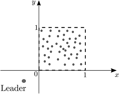
Figure 6: The scheme of the organization of the drum orchestra.

As in Ref. Vlasov et al. (2014), where an example of a geometric organization of oscillators has been treated, we assume that the phase shifts $\beta_{j}$ and $\alpha_{i}$ are proportional to the distances between the oscillator and the leader, thus

$$\beta_{i}=\alpha_{i}={\omega_{s}\over c}\sqrt{(x_{i}-x_{l})^{2}+(y_{i}-y_{l})^{2}}\,,$$ (44)

where $\omega_{s}$ is the central frequency of the original signal (around which the phase approximation was made) and $c$ is the speed of signal propagation. Coupling strengths $B_{j}$ and $A_{i}$ are assumed to be inversely proportional to the square distances between each oscillator and the leader:

$$B_{j}=\frac{W_{B}}{(x_{j}-x_{l})^{2}+(y_{j}-y_{l})^{2}},\quad A_{i}=\frac{W_{A}}{(x_{i}-x_{l})^{2}+(y_{i}-y_{l})^{2}}\;,$$ (45)

here additional initial intensities of the signals $W_{A}$ and $W_{B}$ were added in order to have coupling coefficients of the order $1$ for any distant position of the leader.

Then in the thermodynamic limit the distribution of the coupling parameters can be written as $w(A,B,\alpha,\beta)=w(x,y)$, where all the parameters are the functions (44,45) of the coordinates $(x,y)$ of the 2D plane, except for, perhaps, natural frequencies $\omega$, that can be independently distributed. In our numerical simulations we neglected this, assuming that all oscillators have identical frequencies. The self-consistent approach gives solutions for any given position of the leader outside of the manifold of the oscillators, and for any given value of its own natural frequency. As a measure of synchrony, we will use the order parameter $R$ introduced above in Eq. (43) (if $R$ is close to unity, the regime is synchronous, and if $R$ is small we call this regime asynchronous). The terms “synchronous” and “asynchronous” are used here in order to show the resemblance between the solutions of homogenous and non-homogenous systems. For the latter case, however, the usage of these terms is not entirely correct as can be seen in Fig. 7, where it is impossible to distinguish between the partial synchrony and asynchrony because there is no abrupt transitions, and, except for a small region when all the phases are locked ($R=1$), there is a fraction of locked phases and rotating phases with stationary distribution, that can be named both as partial synchrony and as asynchrony in this case.

Spatial patterns of the average frequencies of the oscillators are shown on the Fig. 8 for positive and negative frequencies of the global field $\Omega$. In both cases there is an area of locked phases, where $\dot{\varphi}=\dot{\phi}=\Omega$, and an area of rotating phases with $\langle\dot{\varphi}\rangle=\text{sign}(\Omega)\sqrt{(\Omega-\omega)^{2}-A^{2}}$.

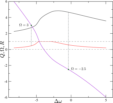
Figure 7: The dependences of the amplitude $Q$ (black curve) and the frequency $\Omega$ (violet curve) of the global field together with the order parameter $R$ (red curve) on the frequency mismatch $\Delta\omega=\omega-\omega_{0}$, obtained self-consistently for the following values of the parameters $x_{l}=-0.1$, $y_{l}=-0.1$ and $W_{A}=W_{B}$, $\omega_{s}/c=1$. Horizontal dashed lines represent $1$ and $0$ on the y-axis. Vertical lines represent the parameters for Fig. 8

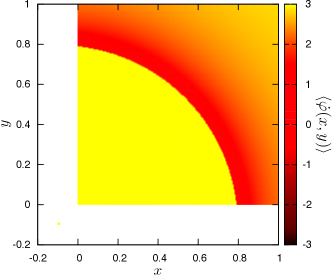
(a) (b)

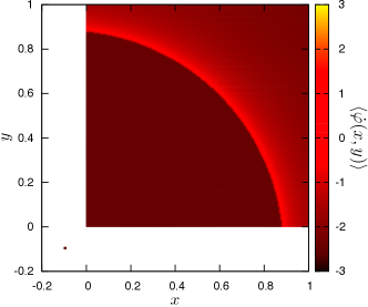
Figure 8: Distributions of the average frequencies of the oscillators for two cases (a) $\Omega=3$ and (b) $\Omega=-2.5$. For the locked phases $\dot{\varphi}=\dot{\phi}=\Omega$ while for the rotating phases $\langle\dot{\varphi}\rangle=\text{sign}(\Omega)\sqrt{(\Omega-\omega)^{2}-A^{2}}$. The parameters are the same as for Fig. 7

This model contains many parameters, varying each one can obtain various regimes. Therefore exhaustive description does not seem possible. While other complex states cannot be a priori excluded, next we will present the solutions that qualitatively coincide with the solutions of the homogenous system.

Fig. 7 shows the dependence of the amplitude $Q$, the frequency $\Omega$ of the global field and the order parameter $R$ on the frequency mismatch $\Delta\omega=\omega-\omega_{0}$ obtained self-consistently, for the case when transitions between synchronous and asynchronous regimes are smooth. For relatively large absolute values $|\Delta\omega|$, the order parameter $R$ is small, but the value of the amplitude $Q$ of the global field is significantly larger than zero. For small negative $\Delta\omega$ the order parameter $R$ is equal to unity, meaning that all the phases are locked, what leads to even larger values of $Q$. The interesting feature is that the maximum value of $Q$ is achieved when $R$ is smaller than unity. The fully asynchronous regime with $R=0$ is not shown on the Fig. 7, however it exists for sufficiently large absolute values of the frequency mismatch $|\Delta\omega|$.

In the second regime, we illustrate the situation when there are two stable steady states (one asynchronous and one synchronous) with a hysteretic transition between them. The dependences of the amplitude $Q$ and the frequency $\Omega$ of the global field on the frequency mismatch $\Delta\omega=\omega-\omega_{0}$ for this case together with the order parameter $R$ are shown in Fig. 9. In these figures we depict both the results obtained by the self-consistent method and by direct numerical simulations. These two are very close (slight differences are due to the finite-size effects and the fact that we stop calculations at a finite time) everywhere except for the area of the hysteresis that can be observed in the neighbourhood of the maximum amplitude of the global field, and when the values of the order parameter $R$ are close to unity. For the large absolute values of the frequency mismatch $|\Delta\omega|$, the order parameter $R$ is small and goes to zero with further increase of $|\Delta\omega|$, what means that the number of locked phases is low and goes to zero with further increasing of $|\Delta\omega|$.

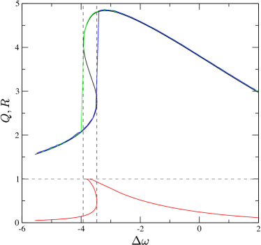
(a) (b)

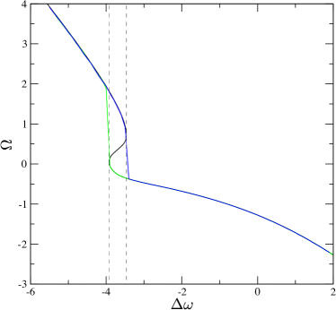
Figure 9: (a) The dependences of the amplitude $Q$ of the global field (black curve represents self-consistent solution, blue and green curves — numeric) and the order parameter $R$ (red curve obtained from self-consistent method) as functions of the frequency mismatch $\Delta\omega=\omega-\omega_{0}$, for the case $x_{l}=-0.1$, $y_{l}=-0.1$ and $W_{A}=0.25W_{B}$, $\omega_{s}/c=1$. (b) The dependences of the frequency $\Omega$ of the global field (black curve from self-consistent approach is mostly hidden but can be seen in the area of hysteresis, blue and green curves from numerics) as functions of the frequency mismatch $\Delta\omega=\omega-\omega_{0}$, for the case $x_{l}=-0.1$, $y_{l}=-0.1$ and $W_{A}=0.25W_{B}$, $\omega_{s}/c=1$. Horizontal dashed line represents $1$ on the y-axis. Vertical dashed lines show the area of hysteresis.

Another regime represents the case when there is one stable synchronous fixed point and one unstable asynchronous fixed point. The results of numerical simulations and the self-consistent method for this case are shown in Fig. 10. For negative and small positive values of $\Delta\omega$, there is a steady solution. Being asynchronous for large negative $\Delta\omega$, it gradually becomes partly synchronous for small negative $\Delta\omega$, and transforms to a synchronous solution ($R=1$) for small positive $\Delta\omega$. As can be seen with the help of numerical simulations, with further increasing of $\Delta\omega$ the steady solution becomes unstable and we observe the oscillating regime (these limit cycle oscillations are illustrated in Fig. 11).

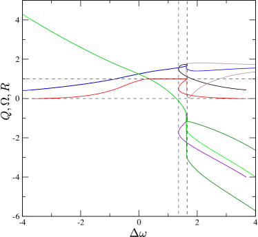
Figure 10: The dependences of the amplitude $Q$ (black curve is obtained self-consistently, blue curve is an average value on the limit cycle obtained numerically and brown curves are minimum and maximum values on the limit cycle) and the frequency $\Omega$ (violet curve — self-consistent solution, light green curve is numerical average over the limit cycle, dark green curves are the minimum and the maximum on the limit cycle) of the global field on the frequency mismatch $\Delta\omega=\omega-\omega_{0}$ together with the order parameter $R$ (red curve obtained from self-consistent method). The following values of the parameters were used $x_{l}=-1$, $y_{l}=-1$ and $W_{A}=W_{B}$, $\omega_{s}/c=1$. Horizontal dashed lines represent $1$ and $0$ on the y-axis. Vertical dashed lines show the area of hysteresis.

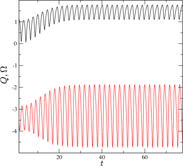
Figure 11: Numerical simulations for the amplitude $Q$ (black curve) and the frequency $\Omega$ (red curve) of the global field as functions of time for $\Delta\omega=\omega-\omega_{0}=3$, for the same values of the parameters as in Fig. (10).

In connection with the interpretation of the model as a “drum orchestra”, the global field represents the signal collected from all the drummers and filtered at the main frequency. This frequency is equal to the frequency of the global field $\Omega$ and the intensity of this filtered collected signal is equal to the amplitude of the global field $Q$. The order parameter $R$ represents the relative amount of drummers oscillating with the same main frequency of the collected signal $\Omega$. Our calculations show that perfect synchrony of the orchestra is not achieved when the intensity of the filtered collected signal is maximum, therefore it is not appropriate to use it as a measure for synchrony of the orchestra.

V Conclusions

In this paper we have performed the analysis of homogeneous and inhomogeneous ensembles of oscillators coupled through a leader by virtue of two methods: the Watanabe-Strogatz approach for identical oscillators, and the self-consistent theory for nonidentical oscillators. While the former method yields also stability of the solutions, in the second approach the stability properties are indicated with the help of direct numerical simulations.

In the homogenous case, the WS approach gives a possibility for a full analytical analysis of the system. The main result is the existence of a hysteretic transition from asynchrony to synchrony for some set of the parameters, while for other sets the transition is not hysteretic. Another distinction from classical Kuramoto-type systems is that the asynchronous solution has a non-zero order parameter.

In the inhomogeneous case, solutions rotating with a constant frequency have been found self-consistently. As an example we consider the case when coupling parameters are determined by the spatial distribution of the oscillators. In this situation the solutions similar to that of the homogeneous system can be found. In this case the stability analysis cannot be performed, but with the help of direct numerical simulations we are able to show which solutions are expected to be stable and which not.

Although our interpretation of the star-type network as a “drum orchestra” is sketchy and of course cannot be applied to real musical performances, the very field of acoustically coupled elements is, in our opinion, one where potential geometric effects on synchronization due to delay in signal propagation could be visible. Indeed, for a rhythm with a 1/2 second period, propagation in air at distance of about 80 m would give a phase shift close to $\pi$, and such distances are not unusual for large drumming sections.

The star-type network considered in this paper is just one example where the coupling can be expressed through a mean field. More generally, there can be a set of global variables (generalized mean fields) that act on oscillators. There are two main types of coupling: (i) the mean field is algebraically expressed through the states of the oscillators, this is the case of the standard Kuramoto model and its generalization to more complex coupling functions; (ii) the global variables are dynamical ones, i.e. there are dynamical equations for the mean fields. To this second class belong situations where the global variables obey linear or nonlinear passive equations (e.g., for Huygens clocks on a common support, the latter can be described as a linear passive oscillator; similarly the common load for an array of Josephson junctions is a passive linear or nonlinear LCR circuit). The star-coupled network above is one where the global field is itself active, i.e. a self-sustained oscillator. We studied only a situation where this central oscillator is of the same type as those in the battery, in particular it is described by a similar phase equation. It would be interesting to study more general setups, where the leader is, e.g., a weakly nonlinear self-sustained oscillator described by the Stuart-Landau equations. Another possible generalization is a system with several global fields. Partially we have touched it, when both leader-mediated and direct Kuramoto-Sakaguchi-type coupling terms have been included. Here of potential interest would be setups with two or more competing leaders, we expect that the analytical approaches developed in this paper could be extended to studies of such problems.

Appendix A Representing the order parameter in terms of Watanabe-Strogatz (WS) global variables

In order to represent the order parameter

$$Z={1\over N}\sum_{j=1}^{N}e^{\text{i}\varphi_{j}}$$ (46)

through the WS variables one should substitute the original phases included as $e^{\text{i}\varphi_{k}}$ with the WS transformation (8) (see Pikovsky and Rosenblum (2011) for details), such that

$$Z={1\over N}\sum_{j=1}^{N}e^{\text{i}\varphi_{j}}={1\over N}\sum_{j=1}^{N}\frac{z+e^{\text{i}(\psi_{j}+\Psi)}}{1+z^{*}e^{\text{i}(\psi_{j}+\Psi)}}.$$ (47)

The expression (47) is rather complex and not applicable for analytical analysis. But there is a special case when this expression becomes extremely simple. First let us use an identity

$$\left(1+z^{*}e^{\text{i}(\psi_{j}+\Psi)}\right)^{-1}=\sum_{l=0}^{\infty}(-z^{*})^{l}e^{\text{i}l(\psi_{j}+\Psi)}.$$ (48)

Using the identity (48) we rewrite the expression (47) for $Z$

$$Z={1\over N}\sum_{j=1}^{N}\left(z+e^{\text{i}(\psi_{j}+\Psi)}\right)\sum_{l=0}^{\infty}(-z^{*})^{l}e^{\text{i}l(\psi_{j}+\Psi)},$$ (49)

or

$$Z=z\left[1+\left(1-|z|^{-2}\right)\sum_{l=1}^{\infty}(-z^{*})^{l}{1\over N}\sum_{j=1}^{N}e^{\text{i}l(\psi_{j}+\Psi)}\right],$$ (50)

Then, in the thermodynamic limit (the number of oscillators goes to infinity), there is one special configuration of constants $\psi$ (the index has been dropped because constants now have continuous distribution) when this expression is simple. Such a configuration is a uniform distribution of constants $\psi$. In this case the order parameter $Z$ is equal to the global variable $z$ (due to the fact that the sums over $j$ in (50) become integrals over the distribution and in the case of the uniform distribution these integrals vanish). Note that the requirement of the uniform distribution of constants $\psi$ is a restriction on initial conditions, but it does not mean that the initial conditions should be also uniformly distributed (because $z(0)$ not necessary should be equal to zero).

Appendix B Special case when $\cos\delta=-1$ and $B=A$

If $\cos\delta=-1$ and $B=A$ then Eqs. (11) transform to

$$\begin{split}\dot{\rho}&=A\frac{1-\rho^{2}}{2}{\rm Re}(e^{\text{i}\Delta\Phi}),\\ \dot{\Delta\Phi}&=\Delta\omega-A\frac{1-\rho^{2}}{2\rho}\,{\rm Im}(e^{\text{i}\Delta\Phi}).\end{split}$$ (51)

Thus in this special case, there are no synchronous steady states, only limit cycle with $\rho=1$ and $\Delta\Phi(t)=\Delta\omega\,t$. The asynchronous steady states could be found from the equations analogous to Eqs. (18), they read

$$\begin{split}\Delta\Phi&=\pm\,\pi/2,\\ 0&=\Delta\omega\mp A\frac{1-\rho^{2}}{2\rho}.\end{split}$$ (52)

Then the steady asynchronous solutions are

$${z_{a}}_{1,2}=\text{sign}(\Delta\omega)\,\text{i}\frac{\,-|\Delta\omega|\mp\sqrt{\Delta\omega^{2}+A^{2}\,}\,}{A}.$$ (53)

From (53) follows that $|{z_{a}}_{1}|>1$ and $|{z_{a}}_{2}|<1$ if $\Delta\omega\neq 0$. And thus there is only one asynchronous steady solution ${z_{a}}_{2}$. After linearization around ${z_{a}}_{2}$ the following linear system is obtained

$$\begin{split}\dot{a}&=-\,\text{sign}(\Delta\omega)\,\sqrt{\Delta\omega^{2}+A^{2}\,}\,b,\\ \dot{b}&=\text{sign}(\Delta\omega)\,|\Delta\omega|a,\end{split}$$ (54)

where $a={\rm Re}(z)$ and $b={\rm Im}(z)-{\rm Im}({z_{a}}_{2})$. Linear system (54) has two eigenvalues:

$${\lambda_{a}}_{2}^{1,2}=\pm\sqrt{-|\Delta\omega|\sqrt{\Delta\omega^{2}+A^{2}\,}\,},$$ (55)

what means that ${z_{a}}_{2}$ is neutrally stable as in the general case when $\sin\delta=0$.

Appendix C The presentation of the solutions for all values of the parameters

Here we present a detailed description of the solution for all three cases. Since we consider only the case when $\cos\xi>0$ (for $\cos\xi=0$ see separate section) and thus $\sin\xi\neq 1$, the solution with stability for $\Delta x>0$ [$\Delta x<0$] is

(i) (Fig. 5(a)) $(2\sin\xi-g)>g$, note that $1>\sin\xi>g\geq 0$ and

$$\left(|\Delta x|-(\sin\xi)\,\frac{|\Delta x|\pm\sqrt{\Delta x^{2}-g(2\sin\xi-g)}\,}{2\sin\xi-g}\right)>0.$$ (56)

$$\begin{split}&{z_{s}}_{1}-sink(stable)node\ [sink(stable)node]\ \ \ \text{and}\\ &{z_{s}}_{2}-source(unstable)node\ [source(unstable)node],\ \ \ \text{if}\ |\Delta x|<\sqrt{g(2\sin\xi-g)\,},\\ \\ &{z_{a}}_{1}-saddle\ [saddle],\ \ {z_{a}}_{2}-stable\ [unstable]\ \ \ \text{and}\\ &{z_{s}}_{1}-sink(stable)node\ [sink(stable)node]\ \ \ \text{and}\\ &{z_{s}}_{2}-source(unstable)node\ [source(unstable)node],\ \ \ \text{if}\ \sqrt{g(2\sin\xi-g)\,}\leq|\Delta x|\leq\sin\xi,\\ \\ &{z_{a}}_{2}-stable\ [unstable]\ \ \ \text{and}\\ &{z_{s}}_{1}-saddle\ [sink(stable)node]\ \ \ \text{and}\\ &{z_{s}}_{2}-source(unstable)node\ [saddle],\ \ \ \text{if}\ \sin\xi<|\Delta x|\leq 1,\\ \\ &{z_{a}}_{2}-stable\ [unstable],\ \ \ \text{and}\\ &|z|=1,\ \text{arg}(z)=\Delta\Phi(t),\ unstable\ [stable]\ limit\ cycle\ \ \ \text{if}\ 1<|\Delta x|.\end{split}$$ (57)

(ii) (Fig. 5(b)) $-g\leq(2\sin\xi-g)\leq g$, so $g\geq\sin\xi\geq 0$ and

$$\left(|\Delta x|-(\sin\xi)\,\frac{|\Delta x|\pm\sqrt{\Delta x^{2}-g(2\sin\xi-g)}\,}{2\sin\xi-g}\right)>0$$ (58)

$$\begin{split}&{z_{s}}_{1}-sink(stable)node\ [sink(stable)node]\ \ \ \text{and}\\ &{z_{s}}_{2}-source(unstable)node\ [source(unstable)node],\qquad\text{if}\ |\Delta x|<\sin\xi,\\ \\ &{z_{a}}_{2}-stable\ [unstable]\ \ \ \text{and}\\ &{z_{s}}_{1}-saddle\ [sink(stable)node]\ \ \ \text{and}\\ &{z_{s}}_{2}-source(unstable)node\ [saddle],\qquad\text{if}\ \sin\xi\leq|\Delta x|\leq 1,\\ \\ &{z_{a}}_{2}-stable\ [unstable],\ \ \ \text{and}\\ &|z|=1,\ \text{arg}(z)=\Delta\Phi(t),\ unstable\ [stable]\ limit\ cycle\ \ \ \text{if}\ 1<|\Delta x|.\end{split}$$ (59)

(iii) (Fig. 5(c)) $(2\sin\xi-g)<-g$, thus $\sin\xi<0$ and

$$\begin{split}\left(|\Delta x|-(\sin\xi)\,\frac{|\Delta x|+\sqrt{\Delta x^{2}-g(2\sin\xi-g)}\,}{2\sin\xi-g}\right)&<0\\ \left(|\Delta x|-(\sin\xi)\,\frac{|\Delta x|-\sqrt{\Delta x^{2}-g(2\sin\xi-g)}\,}{2\sin\xi-g}\right)&>0\end{split}$$ (60)

$$\begin{split}&{z_{a}}_{1}-unstable\ [stable],\ \ {z_{a}}_{2}-stable\ [unstable]\ \ \ \text{and}\\ &{z_{s}}_{1}-saddle\ [saddle]\ \ \ \text{and}\\ &{z_{s}}_{2}-saddle\ [saddle],\qquad\text{if}\ |\Delta x|\leq|\sin\xi|,\\ \\ &{z_{a}}_{2}-stable\ [unstable]\ \ \ \text{and}\\ &{z_{s}}_{1}-saddle\ [sink(stable)node]\ \ \ \text{and}\\ &{z_{s}}_{2}-source(unstable)node\ [saddle],\qquad\text{if}\ |\sin\xi|<|\Delta x|\leq 1,\\ \\ &{z_{a}}_{2}-stable\ [unstable],\ \ \ \text{and}\\ &|z|=1,\ \text{arg}(z)=\Delta\Phi(t),\ unstable\ [stable]\ limit\ cycle\ \ \ \text{if}\ 1<|\Delta x|.\end{split}$$ (61)

Where

$$\begin{split}&{z_{s}}_{1}=e^{\text{i}\left(\frac{\pi}{2}+\arcsin\Delta x-\xi\right)},\\ &{z_{s}}_{2}=e^{\text{i}\left(-\frac{\pi}{2}-\arcsin\Delta x-\xi\right)},\end{split}$$ (62)

and if $2\sin\xi-g\neq 0$

$$\begin{split}&{z_{a}}_{1}=\text{sign}(\Delta x)\,\text{i}\frac{|\Delta x|+\sqrt{\Delta x^{2}-g(2\sin\xi-g)}}{2\sin\xi-g},\\ &{z_{a}}_{2}=\text{sign}(\Delta x)\,\text{i}\frac{|\Delta x|-\sqrt{\Delta x^{2}-g(2\sin\xi-g)}}{2\sin\xi-g},\end{split}$$ (63)

or if $2\sin\xi-g=0$

$$\begin{split}&{z_{a}}_{1}=\text{sign}(\Delta x)\,\text{i}\frac{g}{2|\Delta x|},\\ &{z_{a}}_{2}=-\,\text{sign}(\Delta x)\,\text{i}\frac{g}{2|\Delta x|}.\end{split}$$ (64)

References

- Acebrón et al. (2005) J. A. Acebrón, L. L. Bonilla, C. J. P. Vicente, F. Ritort, and R. Spigler, Rev. Mod. Phys. 77, 137 (2005).
- Pikovsky and Rosenblum (2015) A. Pikovsky and M. Rosenblum, arXiv:1504.06747 [nlin.AO] (2015).
- Kuramoto (1975) Y. Kuramoto, in International Symposium on Mathematical Problems in Theoretical Physics, edited by H. Araki (Springer Lecture Notes Phys., v. 39, New York, 1975) p. 420.
- Kuramoto (1984) Y. Kuramoto, Chemical Oscillations, Waves and Turbulence (Springer, Berlin, 1984).
- Watanabe and Strogatz (1993) S. Watanabe and S. H. Strogatz, Phys. Rev. Lett. 70, 2391 (1993).
- Watanabe and Strogatz (1994) S. Watanabe and S. H. Strogatz, Physica D 74, 197 (1994).
- Ott and Antonsen (2008) E. Ott and T. M. Antonsen, CHAOS 18, 037113 (2008).
- Wiesenfeld et al. (1996) K. Wiesenfeld, P. Colet, and S. H. Strogatz, Phys. Rev. Lett. 76, 404 (1996).
- Pikovsky (2013) A. Pikovsky, Phys. Rev. E 88, 032812 (2013).
- Pikovsky and Rosenblum (2009) A. Pikovsky and M. Rosenblum, Physica D 238(1), 27 (2009).
- Kazanovich and Borisyuk (2003) Y. Kazanovich and R. Borisyuk, Prog. Theor. Phys. 110, 1047 (2003).
- Burylko et al. (2012) O. Burylko, Y. Kazanovich, and R. Borisyuk, Physica D 241, 1072 (2012).
- Kazanovich et al. (2013) Y. Kazanovich, O. Burylko, and R. Borisyuk, Physica D 261, 114 (2013).
- Vlasov et al. (2014) V. Vlasov, E. E. N. Macau, and A. Pikovsky, Chaos: An Interdisciplinary Journal of Nonlinear Science 24, 023120 (2014).
- Vlasov, Zou and Pereira (2015) V. Vlasov, Y. Zou, and T. Pereira, Phys. Rev. E 92, 012904 (2015).
- Tsang et al. (1991) K. Y. Tsang, R. E. Mirollo, S. H. Strogatz, and K. Wiesenfeld, Physica D 48, 102 (1991).
- Golomb et al. (1992) D. Golomb, D. Hansel, B. Shraiman, and H. Sompolinsky, Phys. Rev. A 45, 3516 (1992).
- Swift et al. (1992) J. W. Swift, S. H. Strogatz, and K. Wiesenfeld, Physica D 55, 239 (1992).
- Vlasov and Pikovsky (2013) V. Vlasov and A. Pikovsky, Phys. Rev. E 88, 022908 (2013).
- Pikovsky and Rosenblum (2011) A. Pikovsky and M. Rosenblum, Physica D 240, 872 (2011).
- Marvel et al. (2009) S. A. Marvel, R. E. Mirollo, and S. H. Strogatz, Chaos 19, 043104. (2009).
- Roberts and Quispel (1992) J. A. G. Roberts and G. R. W. Quispel, Physics Reports 216, 63 (1992).
- Politi et al. (1986) A. Politi, G. L. Oppo, and R. Badii, Phys. Rev. A 33, 4055 (1986).