Cascading Edge Failures: A Dynamic Network Process

Abstract

This paper considers the dynamics of edges in a network. The Dynamic Bond Percolation (DBP) process models, through stochastic local rules, the dependence of an edge $(a,b)$ in a network on the states of its neighboring edges. Unlike previous models, DBP does not assume statistical independence between different edges. In applications, this means for example that failures of transmission lines in a power grid are not statistically independent, or alternatively, relationships between individuals (dyads) can lead to changes in other dyads in a social network. We consider the time evolution of the probability distribution of the network state, the collective states of all the edges (bonds), and show that it converges to a stationary distribution. We use this distribution to study the emergence of global behaviors like consensus (i.e., catastrophic failure or full recovery of the entire grid) or coexistence (i.e., some failed and some operating substructures in the grid). In particular, we show that, depending on the local dynamical rule, different network substructures, such as hub or triangle subgraphs, are more prone to failure.

PACS numbers

I Introduction

In 2003, the failure of a single power line triggered a series of cascading failures throughout the Northeastern United States and Southeastern Canada Minkel (2008). Connectivity of the power grid led to an uncontrollable propagation of failures that resulted in over 50 millions customers losing power. Similarly, the rapid spread of infection during epidemics is due to contacts between individuals of a population. These phenomena are rare and difficult to study via experiments. Due to their scale, they are also expensive to simulate. It is therefore advantageous to be able to study such phenomena analytically.

Cascading failures and epidemics can be modeled as network processes —dynamical processes whose substrate is a particular network structure. It is of interest to understand the dynamics of such processes, particularly the impact of the network structure Jackson (2008); Newman (2010). In some applications such as epidemiology, where nodes represent individuals, it is more intuitive to study network processes on nodes Eames and Keeling (2002); Zhang and Moura (2014, 2015). This means that the state of each node changes according to deterministic or stochastic dynamics often depending on the states of the nodes’ neighbors. This inclusion couples the evolution of each node with that of all the other nodes in the network, resulting in a complex dynamical system. For modeling phenomena such as cascading failures of transmission lines in the power grid or the evolution of relationships, called dyads, in social networks, it is more appropriate to study edge-centric network processes where the edges change state according to some dynamics.

Dynamic edge models have been used in computational sociology to study the time evolution of dyads Wasserman (1980); Leenders (1995); Snijders (2005); Pepyne (2007). However, some models assume that the dynamics of different dyads are statistically independent. These models can not capture effects such as triadic closure, where friendships are more likely to form between individuals with common neighbors Granovetter (1973). Alternatively, models try to capture interdependencies by incorporating knowledge of network structure into the dynamics of a dyad. This assumes that individual dyads have full knowledge of the overall network structure, which may not be feasible in practice.

The bond percolation model from statistical mechanics has been used to study the robustness and resilience of network structures to stochastic bond (i.e., edge) removals Broadbent and Hammersley (1957); Newman (2010); Callaway et al. (2000). However, the standard percolation model is not a network process, as it does not model dynamical evolution of bond states over time Steif (2009). Additionally, the bond percolation model assumes that the size of the network is infinite, and account for the topology only through the degree distribution and not higher order degree correlations. Lastly, percolation is a macroscopic model; it characterizes global properties such as the percentage of removed components, but can not provide information on microscopic properties such as probability that a set of bonds is removed.

The Dynamic Bond Percolation (DBP) model we present in this paper differs from previous models by the inclusion of local coupling dependencies in time between edges as represented by a heterogenous network structure. Each edge in a network can be in one of two states: open and closed. The dynamics of edges are no longer independent as an edge $(a,b)$ changes state according to a stochastic rule depending only on the states of its local neighboring edges. For example, this means that the failure rate of a transmission line is affected by the failures of other transmission lines. Alternatively, the formation of friendship links between individuals $a$ and $b$ depends on the other relationships of $a$ and $b$.

The state of DBP at time $t$ is the collection of the states of all the edges at time $t$. We show that the probability distribution over the states of DBP reaches an equilibrium distribution. For certain local rules, we can compute this distribution explicitly for any finite-size, unweighted, undirected network structure, unlike previous models that approximate the underlying network by simpler structures (e.g., complete graphs) or infinite-size networks (i.e., mean-field approximation) Liggett (1999); Barrat et al. (2008). Analysis of the equilibrium distribution informs us of the emergence of global behavior. For example, in certain parameter regimes, the most probable network state at equilibrium is that of consensus, denoting either complete failure or complete recovery of all transmission lines. In other parameter regimes, it provides information about the subset of transmission lines more prone to cascading failures or more likely to form relationships. We will see that these effects depend on the local dynamical rules.

When the imbalance between node $a$ and node $b$ does not matter, the critical edges tend to belong to star subgraphs (i.e., hub structures). Whereas critical edges tend to belong to triangle subgraphs and other network structures (e.g., $P_{3}$ or $P_{4}$, see Section III.1) when imbalance or mutual relationships matter. We illustrate our analysis within two real-world networks: 118-node IEEE test bus power grid Christie (1993) and 198-node social network Weeks et al. (2002).

Section II explains the Dynamic Bond Percolation process in detail. Section III derives the closed-form equilibrium distribution for 3 different dynamical rules. Section IV describes the Most-Probable Network Problem. Section V through Section VII analyzes the solution space of the Most-Probable Network Problem for the different parameter regimes. Section VIII concludes the paper.

II Dynamic Bond Percolation Process

Consider a population of $N$ individuals or components represented as nodes in a network. The adjacency matrix, $\mathbf{A}_{\max}$, describes the largest set of potentially open or closed bonds between the nodes. We will refer to the network represented by $\mathbf{A}_{\max}$ the maximal network. For example, the maximal network may be a representation of the underlying power grid or a social network between $N$ individuals. We assume that the maximal network is a simple, connected, undirected graph. Let $E_{\max}$ denote the set of edges and $V_{\max}$ denote the set of nodes in the maximal network respectively. Figure 1 shows an example of a maximal network.

Edges in the maximal network may change state over time. For instance, transmission lines in the power grid can fail, social ties between individuals can weaken or strengthen with time. We are particularly interested in scenarios where there is a contagion aspect to the dynamical process: a single transmission line failure can lead to other line failures such as in blackouts.

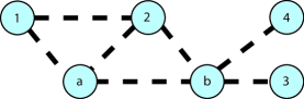
Figure 1: Maximal network represented by $\mathbf{A}_{\max}$. Dashed edges (i.e., bonds) are the only possible edges in the network.

In this paper, we present the Dynamic Bond Percolation (DBP) process, a dynamical extension of the bond percolation model Broadbent and Hammersley (1957). Edges in the maximal network open or close according to stochastic dynamical rules specified by DBP. We assume that the close of an edge depends on the state of the neighboring edges, thereby coupling the underlying network topology with the process dynamics. In applications, DBP can be used to model cascading failures of transmission lines in the power grid or the formation and dissolution of ties in a social network. Figure 3 shows a possible realization of the DBP process on the maximal network shown in Figure 1.

The state of the DBP process at time $t\geq 0$, $A(t)$, is represented by the $N\times N$ adjacency matrix $\mathbf{A}$, where

$$\mathbf{A}_{i,j}= 1\text{ if edge $(a,b)$ is close}$$

$$= 0\text{ if edge $(a,b)$ is open}.$$

We will call $\mathbf{A}$ the network state. The set of nodes in the network state $V(\mathbf{A})=V_{\max}$. The set of edges in the network state corresponds to the set of closed edges in the maximal network; therefore, $E(\mathbf{A})\subseteq E_{\max}$. The space of all possible network states is $\mathcal{A}$. Since each edge in the maximal network can be either open or closed, then $|\mathcal{A}|=2^{|E_{\max}|}$. DBP makes the following assumptions:

Assumption 1: Network states that contain edges not in $E_{\max}$ are invalid. For example, with respect to the maximal network in Figure 1, the network state in Figure 2 is not valid since edge $(2,4)$ is not in the maximal network.

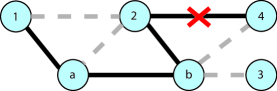
Figure 2: Invalid network state. Edge (2,4) is not in the maximal network and can not change state. Solid edges are closed. Dashed edges are open.

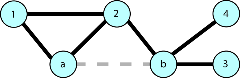
(a) $X(t_{1})$

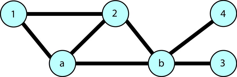
(b) $X(t_{2})$

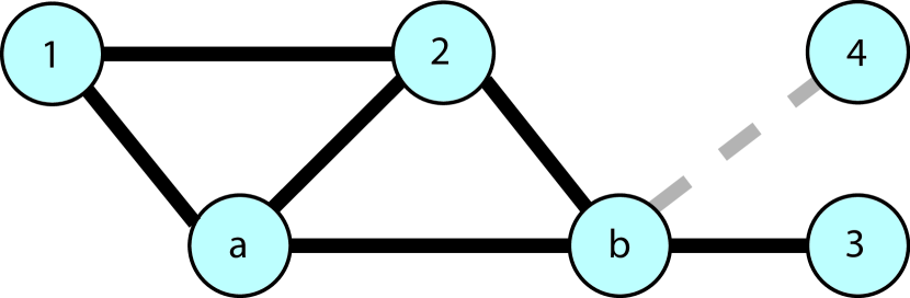
(c) $X(t_{3})$

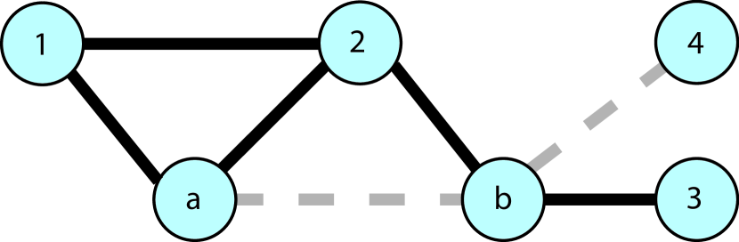
(d) $X(t_{4})$

Figure 3: Example evolution of $A(t)$. Solid edges are closed. Dashed edges are open.

Assumption 2: Multiple edge opening or closure can not occur simultaneously. Only one edge changes state per transition.

Assumption 3: The time it takes for an edge $(a,b)$ to go from close to open (e.g., $t_{4}-t_{3}$ as in Figure 3) is exponentially distributed with rate

$$q(\mathbf{A},T_{a,b}^{-}\mathbf{A})=\mu^{\prime}.$$ (1)

This means that the probability that edge $(a,b)$ switches from close to open $\Delta t$ time units in the future is

$$P(A(t+\Delta t)=T_{a,b}^{-}\mathbf{A}\mid A(t)=\mathbf{A})\approx\mu^{\prime}\Delta t+o(\Delta t),$$

where $o(\cdot)$ is the little-o notation. We call $\mu^{\prime}>0$ the edge opening rate. DBP assumes that $\mu^{\prime}$ is the same for all closed edges. For applications where edge opening is rare, $\mu^{\prime}$ can be arbitrarily small as long as it is not 0.

Assumption 4: The time it takes for an edge $(a,b)$ to go from open to close (e.g., $t_{2}-t_{1}$ as in Figure 3) is exponentially distributed with rate

$$q(\mathbf{A},T_{a,b}^{+}\mathbf{A})=\lambda^{\prime}\gamma^{\prime f(\mathcal{N}_{a},\mathcal{N}_{b})},$$ (2)

where $\mathcal{N}_{a}$ and $\mathcal{N}_{b}$ denotes the set of closed edges connected to node $a$ and the set of closed edges connected to node $b$ in network state $\mathbf{A}$, respectively. We call the function $f(\mathcal{N}_{a},\mathcal{N}_{b})$ the cascade function. It captures how the edge closure rate of $(a,b)$ depends on the local neighborhood of edge $(a,b)$. In this paper, we consider the following cascade functions:

1. SUD-DBP (Sum-Dependent Dynamic Bond Percolation):

   $$f(\mathcal{N}_{a},\mathcal{N}_{b})=|\mathcal{N}_{a}|+|\mathcal{N}_{b}|$$ (3)

2. TRI-DBP (Triangle-Dependent Dynamic Bond Percolation):

   $$f(\mathcal{N}_{a},\mathcal{N}_{b})=|\mathcal{N}_{a}\cap\mathcal{N}_{b}|.$$ (4)

3. POD-DBP (Product-Dependent Dynamic Bond Percolation):

   $$f(\mathcal{N}_{a},\mathcal{N}_{b})=|\mathcal{N}_{a}||\mathcal{N}_{b}|.$$ (5)

SUD-DBP assumes that the closure rate of an edge depends on the sum of the number of closed neighboring edges. POD-DBP assumes that the closure rate depends on the product of the number of closed neighboring edges. These model different dynamics because POD-DBP implicitly accounts for imbalance between the number of closed edges on node $a$, $|\mathcal{N}_{a}|$, and node $b$, $|\mathcal{N}_{b}|$. For example, consider the two scenarios in Figure 4. Under SUD-DBP, the closure rate of edge $(a,b)$ is $\lambda^{\prime}\gamma^{\prime 6}$ for both Scenarios A and B. Under POD-DBP, the closure rate of edge $(a,b)$ is $\lambda^{\prime}\gamma^{\prime 9}$ for Scenario A and $\lambda^{\prime}\gamma^{\prime 5}$ for Scenario B.

TRI-DBP assumes that the closure rate of an edge depends on the number of closed neighboring edges sharing a common agent. This comes from the concept of triadic closure, which states that, for 3 agents $a,b$, and $c$, if there is a connection between $(a,b)$ and $(a,c)$, then it is more likely that there is a connection between $(b,c)$ Brandes et al. (2013). Under TRI-DBP, the closure rate of edge $(a,b)$ is $\lambda^{\prime}$ for both Scenario A and $\lambda^{\prime}\gamma^{\prime}$ for Scenario B.

When $f(\mathcal{N}_{a},\mathcal{N}_{b})=0$, the transition rate $q(\mathbf{A},T_{a,b}^{+}\mathbf{A})=\lambda^{\prime}$. This means that it it is possible for an edge $(a,b)$ to close independent of the state of neighboring edges. Therefore, we consider $\lambda^{\prime}$ to be the spontaneous edge closure rate and $\gamma^{\prime}$ to be the cascading edge closure rate.

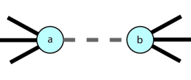
(a) Scenario A: $|\mathcal{N}_{a}|=3,|\mathcal{N}_{b}|=3$.

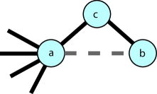
(b) Scenario B: $|\mathcal{N}_{a}|=5,|\mathcal{N}_{b}|=1$.

Figure 4: Different edge removal scenarios. Solid edges are closed. Dashed edges are open.

Since the transition rates are not time dependent, DBP is a time-homogenous process. Since the model assumes both spontaneous edge opening and close, there is no absorbing state. Under the stated assumptions, the Dynamic Bond Percolation model, $\{A(t),t\geq 0\}$, is an irreducible, continuous-time Markov process with finite state space, $\mathcal{A}=\{\mathbf{A}\}$; each state in the Markov process corresponds to a potential network state $\mathbf{A}$. The dimension of the configuration space is $|\mathcal{A}|=2^{|E_{\max}|}$.

III Time-Asymptotic Behavior

While it is difficult to completely characterize the dynamics of the Dynamic Bond Percolation process, its time-asymptotic behavior $\left(\text{i.e., }\lim_{t\to\infty}A(t)\right)$ can be studied using its equilibrium distribution, $\pi$. The equilibrium distribution of DBP is a probability mass function (PMF) over $\mathcal{A}$. Since DBP is a finite-state, continuous-time Markov process, the equilibrium distribution $\pi$ is unique Kelly (1979). It can be found by solving the left eigenvalue-eigenvector problem

$$\pi\mathbf{Q}=0,$$

where $\mathbf{Q}$ is the transition rate matrix, also known as the infinitesimal matrix Norris (1998).

The matrix $\mathbf{Q}$ characterizes the transition rates between all the states in $\mathcal{A}$ using (1), (2). For DBP, it is an asymmetric $2^{|E_{\max}|}\times 2^{|E_{\max}|}$ matrix. Element $\mathbf{Q}_{ij}$ corresponds to the transition rate between 2 states $\mathbf{i},\mathbf{j}\in\mathcal{A}$ where $i$ and $j$ are decimal scalar representations of the network states $\mathbf{i}$ and $\mathbf{j}$, respectively.

The equilibrium distribution of a continuous-time Markov process is the left eigenvector of the transition rate matrix corresponding to the zero eigenvalue. However, the challenge of finding $\pi$ is that the dimensions of $\mathbf{Q}$ scales exponentially with the total number of edges in the maximal network, $|E_{\max}|$. This makes computing the equilibrium distribution prohibitively expensive for large networks. In the next section, we will show that we can avoid this computation for SUD-DBP, TRI-DBP, and POD-DBP by finding the equilibrium distribution, $\pi$, up to a constant, in closed form.

III.1 Review of Graph Theoretic Concepts

First, we review graph theory terms necessary for the rest of the paper West (1996); Jackson (2008).

Definition III.1.

A walk is a list $v_{0},e_{1},v_{1},e_{2},\ldots,e_{k},v_{k}$ of vertices and edges. The length of the walk is the number of edges in the list. The number of walks in an undirected graph from node $i$ to node $j$ of length $k$ is

$$(\mathbf{A}^{k})_{i,j},$$

where $\mathbf{A}^{k}$ is the adjacency matrix of an undirected, unweighted graph raised to the $k$th power.

Definition III.2.

A path is a walk where all the vertices are distinct (although some literature does not make this distinction between paths and walks). A graph that is a path is called a path graph and written as $P_{n}$, where $n$ is the number of vertices (not edges) in the path. By convention, the path graph $P_{n}$ is equivalent to a path of length $n-1$. Figure 5(a) shows the $P_{3}$ subgraph and Figure 5(c) shows the $P_{4}$ subgraph.

Definition III.3.

A cycle is a path where the endpoints $v_{0}=v_{k}$. A graph that is a cycle is called a cycle graph and written as $C_{n}$, where $n$ is the number of vertices (not edges) in the cycle. By convention, the cycle graph $C_{n}$ is equivalent to a cycle of length $n$. Figure 5(b) shows the $C_{3}$ subgraph. $C_{3}$ subgraphs are also called triangles.

(a) $P_{3}$ graph

(b) $C_{3}$ graph

(c) $P_{4}$ graph

(d) $S_{6}(4)$ star graph

Figure 5: $P_{3}$, $C_{3}$, $P_{4}$ and $S_{6}(4)$ subgraphs

Definition III.4.

A star graph, $S_{n}(i)$, has $n$ vertices that are only connected to the center vertex $i$. Figure 5(d) shows the $S_{6}(4)$ subgraph.

Definition III.5.

West (1996) A matching, $\mathcal{M}$, of the graph $G(V,E)$, also called the Independent Edge Set, is a subset of edges $E$ such that no vertex in $V$ is incident to more than one edge in $\mathcal{M}$; see Figure 6(a). Maximum Matching is a matching with the maximum number of edges; see Figure 6(b).

The number of edges in the maximum matching is known as the matching number, $\nu(G)$.

In this paper, we introduce a generalization to the matching set.

Definition III.6.

A star matching, $\mathcal{S}$, of the graph $G(V,E)$, is a subset of edges $E$ such that these edges form a collection of disconnected star graphs; see Figure 6(c). Maximum star matching is a star matching with the maximum number of edges; see Figure 6(d). Note that $\mathcal{M}\subset\mathcal{S}$.

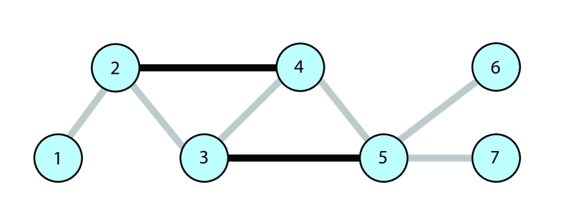
(a) Matching: $\{(2,4),(3,5)\}$

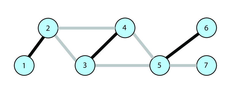
(b) Max Matching: $\{(1,2),(3,4),(5,6)\}$

(c) Star Matching: $\{(1,2),(2,3),(4,5),(5,6)\}$

(d) Max Star Matching: $\{(1,2),(3,5),(4,5),(5,6),(6,7)\}$

Figure 6: Matching and Star Matching

III.2 Reversibility and Equilibrium Distribution

Some Markov processes possess the property that the process forward in time is statistically equivalent to the process backward in time. These Markov processes are called reversible Markov processes. The following theorem is important in deriving the stationary distribution of a reversible Markov process:

Theorem III.7 (From Kelly (1979)).

A stationary Markov process is reversible if and only if there exists a collection of positive number $\pi(j),j\in\mathcal{L}$, summing to unity that satisfy the detailed balance conditions

$$\pi(j)q(j,k)=\pi(k)q(k,j),\quad j,k,\in\mathcal{L},$$

where $q(\cdot,\cdot)$ is the transition rate of the Markov process. When there exists such a collection $\pi(j),j\in\mathcal{L}$, it is the equilibrium distribution of the process.

Using this theorem, we will show that the equilibrium distributions for SUD-DBP, POD-DBP, and TRI-DBP have the form:

$$\pi(\mathbf{A})=\frac{1}{Z}\left(\frac{\lambda^{\prime}}{\mu^{\prime}}\right)^{\prime|E(\mathbf{A})|}\gamma^{\prime g(E(\mathbf{A}))},\quad\mathbf{A}\in\mathcal{A},$$ (6)

where the partition function, $Z$, is

$$Z=\sum_{\mathbf{A}\in\mathcal{A}}\left(\frac{\lambda^{\prime}}{\mu^{\prime}}\right)^{|E(\mathbf{A})|}\gamma^{\prime g(E(\mathbf{A}))}.$$ (7)

The exponent $|E(\mathbf{A})|$ is the total number of closed edges in a network state, and $g(E(\mathbf{A}))$ is the number of special network structures induced by the set of closed edges $E(\mathbf{A})$. These special network structures are derived for SUD-DBP, POD-DBP, TRI-DBP in sections III.3,  III.5, and III.4, respectively.

The equilibrium distribution is the product of three terms: the partition function $Z$, a structure-free term, and a structure-dependent term that depends on the maximal network. Let $E(\mathbf{A})$ denote the set of closed edges in network state $\mathbf{A}$. The term $\left(\frac{\lambda^{\prime}}{\mu^{\prime}}\right)^{|E(\mathbf{A})|}$ is structure-free because it depends only on the number of close edges in network state whereas the term $\gamma^{\prime g(E(\mathbf{A}))}$ depends on the underlying maximal network topology.

III.3 (SUD-DBP) Sum-Dependent Dynamic Bond Percolation Model

Theorem III.8.

The Sum-Dependent Dynamic Bond Percolation model, $\{A(t),t\geq 0\}$, is a reversible Markov process and the equilibrium distribution is

$$\pi(\mathbf{A})=\frac{1}{Z}\left(\frac{\lambda^{\prime}}{\mu^{\prime}}\right)^{|E(\mathbf{A})|}\gamma^{\prime g(E(\mathbf{A}))},\quad\mathbf{A}\in\mathcal{A},$$ (8)

where $g(E(\mathbf{A}))$ it the number of $P_{3}$ subgraphs induced by the set of closed edges $E(\mathbf{A})$.

The number of close edges in a network state is

$$|E(\mathbf{A})|=\frac{\mathbf{1}^{T}\mathbf{A}\mathbf{1}}{2},$$

where $\mathbf{1}=[1,1,\ldots,1]^{T}$.

The number of $P_{3}$ subgraphs induced by the edges $E(\mathbf{A})$ in a network state is

$$g(E(\mathbf{A}))=\sum_{i=1}^{N}\sum_{j>i}(\mathbf{A}^{2})_{i,j}=\sum_{i=1}^{N}\binom{k_{i}}{2},$$ (9)

where $k_{i}=\sum_{j=1}^{N}\mathbf{A}_{ij}$ and is the number of closed edges at node $i$. The derivation of the closed-from equation of $g(E(\mathbf{A}))$ is in Appendix A

In the SUD-DBP model, the sufficient statistics are the total number of close edges and the total number of paths of length 2 (i.e., the number of $P_{3}$ subgraphs) induced by the closed edges. The number of $P_{3}$ subgraphs induced by the closed edges is related also to the degree of the network state $\mathbf{A}$. Surprisingly, this means that a sufficient statistic of a process where edges change state in time is a nodal characteristic.

Proof.

We prove that the equilibrium distribution $\pi(\mathbf{A})$ of the SUD-DBP is given by (8).

By Theorem III.7, $\pi(\mathbf{A})$ satisfies the detailed balance equations:

$$\pi(\mathbf{A})q(\mathbf{A},T^{+}_{a,b}\mathbf{A})=\pi(T^{+}_{a,b}\mathbf{A})q(T^{+}_{a,b}\mathbf{A},\mathbf{A})$$ (10)

and

$$\pi(\mathbf{A})q(\mathbf{A},T^{-}_{a,b}\mathbf{A})=\pi(T^{-}_{a,b}\mathbf{A})q(T^{-}_{a,b}\mathbf{A},\mathbf{A}).$$ (11)

We prove (10) first.

Let $T^{+}_{a,b}\mathbf{A}$ denote the network state that is the same as network state $\mathbf{A}$ except edge $(a,b)$ switches from open to close. According to the transition rate in (2) for SUD-DBP (3),

$$q(\mathbf{A},T^{+}_{a,b}\mathbf{A})=\lambda^{\prime}\gamma^{\prime k_{a}+k_{b}},$$

where $k_{a}=|\mathcal{N}_{a}|=\sum_{i=1}^{N}\mathbf{A}_{ai}$ and $k_{b}=|\mathcal{N}_{b}|=\sum_{i=1}^{N}\mathbf{A}_{bi}$ are the number of closed edges incident at node $a$ and $b$, respectively.

According to the equilibrium distribution of SUD-DBP (8), the equilibrium probability of network state $\mathbf{A}$ is

$$\pi(\mathbf{A})=\frac{1}{Z}\left(\frac{\lambda^{\prime}}{\mu^{\prime}}\right)^{|E(\mathbf{A})|}\gamma^{\prime g(E(\mathbf{A}))},$$

where $g(E(\mathbf{A}))$ is the number of $P_{3}$ subgraphs induced by the set of closed edges $E(\mathbf{A})$. The LHS of (10) is

$$\begin{split}&\pi(\mathbf{A})q(\mathbf{A},T^{+}_{a,b}\mathbf{A})\\ &=\frac{1}{Z}\left(\frac{\lambda^{\prime}}{\mu^{\prime}}\right)^{|E(\mathbf{A})|}\gamma^{\prime g(E(\mathbf{A}))}\left(\lambda^{\prime}\gamma^{\prime k_{a}k_{b}}\right)\\ &=\frac{1}{Z}\left(\frac{\lambda^{\prime|E(\mathbf{A})|+1}}{\mu^{\prime|E(\mathbf{A})|}}\right)\gamma^{\prime g(E(\mathbf{A}))+k_{a}+k_{b}}.\end{split}$$ (12)

According to the transition rate in (1),

$$q(T^{+}_{a,b}\mathbf{A},\mathbf{A})=\mu^{\prime}.$$

Recognize that by definition, $|E(T^{+}_{a,b}\mathbf{A})|=1+|E(\mathbf{A})|$. Consider the closure of edge $(a,b)$. This means that the number of paths of length 2 from any node in $\mathcal{N}_{a}$ to the node $b$ is $k_{a}$ and the number of paths of length 2 from the node $a$ to any node in $\mathcal{N}_{b}$ in $k_{b}$. Therefore, $g(E(T^{+}_{a,b}\mathbf{A}))=g(E(\mathbf{A}))+k_{a}+k_{b}$.

The RHS of (10) is

$$\begin{split}&\pi(T^{+}_{a,b}\mathbf{A})q(T^{+}_{a,b}\mathbf{A},\mathbf{A})\\ &=\frac{1}{Z}\left(\frac{\lambda^{\prime}}{\mu^{\prime}}\right)^{|E(T^{+}_{a,b}\mathbf{A})|}\gamma^{\prime g(E(T^{+}_{a,b}\mathbf{A}))}\mu^{\prime}\\ &=\frac{1}{Z}\left(\frac{\lambda^{\prime|E(\mathbf{A})|+1}}{\mu^{\prime|E(\mathbf{A})|}}\right)\gamma^{\prime g(E(\mathbf{A}))+k_{a}+k_{b}}.\end{split}$$ (13)

The LHS and RHS of (10) are equivalent. Similar reasoning holds for (11). Since the detailed balance equations are satisfied by (8), Theorem III.7 proves Theorem III.8.

∎

III.4 (TRI-DBP) Triangle-Dependent Dynamic Bond Percolation Model

Theorem III.9.

The Triangle-Dependent Dynamic Bond Percolation model, $\{A(t),t\geq 0\}$, is a reversible Markov process and the equilibrium distribution is

$$\pi(\mathbf{A})=\frac{1}{Z}\left(\frac{\lambda^{\prime}}{\mu^{\prime}}\right)^{|E(\mathbf{A})|}\gamma^{\prime g(E(\mathbf{A}))},\quad\mathbf{A}\in\mathcal{A},$$ (14)

where $g(E(\mathbf{A}))$ it the number of $C_{3}$ subgraphs induced by the set of closed edges $E(\mathbf{A})$.

The number of close edges in a network state is

$$|E(\mathbf{A})|=\frac{\mathbf{1}^{T}\mathbf{A}\mathbf{1}}{2},$$

where $\mathbf{1}=[1,1,\ldots,1]^{T}$.

The number of $C_{3}$ subgraphs induced by the edges $E(\mathbf{A})$ in a network state is West (1996)

$$g(E(\mathbf{A}))=\sum_{i=1}^{N}\frac{(\mathbf{A}^{3})_{i,i}}{6}.$$ (15)

In the TRI-DBP model, the sufficient statistics are the total number of close edges and the total number of triangles (i.e., the number of $C_{3}$ subgraphs) induced by the closed edges. The proof for Theorem III.9 follows the same steps as the proof for Theorem III.8 except 1) the transition rate $q(\mathbf{A},T^{+}_{a,b}\mathbf{A})$ for TRI-DBP is given by (4), and 2) the number of $C_{3}$ subgraphs $g(E(T^{+}_{a,b}\mathbf{A}))=|\mathcal{N}_{a}\cap\mathcal{N}_{b}|+g(E(\mathbf{A}))$.

III.5 (POD-DBP) Product-Dependent Dynamic Bond Percolation Model

Theorem III.10.

The Product-Dependent Dynamic Bond Percolation model, $\{A(t),t\geq 0\}$, is a reversible Markov process and the equilibrium distribution is

$$\pi(\mathbf{A})=\frac{1}{Z}\left(\frac{\lambda^{\prime}}{\mu^{\prime}}\right)^{|E(\mathbf{A})|}\gamma^{\prime g(E(\mathbf{A}))},\quad\mathbf{A}\in\mathcal{A},$$ (16)

where $\mathbf{A}$ is the adjacency matrix, $g(E(\mathbf{A}))$ is the number of triangles $C_{3}$, and the paths of length 3, $P_{4}$ formed by the set of closed edges, $E(\mathbf{A})$.

The number of close edges, $|E(\mathbf{A})|$, is

$$|E(\mathbf{A})|=\frac{\mathbf{1}^{T}\mathbf{A}\mathbf{1}}{2},$$

where $\mathbf{1}=[1,1,\ldots,1]^{T}$.

The number of $C_{3}$ and $P_{4}$ subgraphs is

$$\begin{split}&g(E(\mathbf{A}))=\sum_{i=1}^{N}\frac{(\mathbf{A}^{3})_{i,i}}{6}+\\ &\sum_{i=1}^{N}\sum_{j>i}\left[(\mathbf{A}^{3})_{i,j}-(\mathbf{A}_{i,j})\left((\mathbf{A}^{2})_{i,i}+\sum_{k=1,k\neq i,j}^{N}\mathbf{A}_{k,j}\right)\right].\end{split}$$ (17)

The derivation of the closed-from equation of $g(E(\mathbf{A}))$ is in Appendix B.

In the POD model, the sufficient statistics are the total number of closed edges and the total number of $C_{3}$ and $P_{4}$ subgraphs induced by the closed edges. The POD model and the SUD model do not have the same sufficient statistics. The proof for Theorem III.10 follows the same steps as the proof for Theorem III.8 except 1) the transition rate $q(\mathbf{A},T^{+}_{a,b}\mathbf{A})$ for POD-DBP is given by (5), and 2) the number of paths of length 3 from any node in $\mathcal{N}_{a}$ to any node in $\mathcal{N}_{b}$ through edge $(a,b)$ is $|\mathcal{N}_{a}||\mathcal{N}_{b}|$. Therefore $g(E(T^{+}_{a,b}\mathbf{A}))=k_{a}k_{b}+g(E(\mathbf{A}))$.

IV Critical Structures and the Most-Probable Network Problem

In the second part of the paper, we will use DBP to study critical structures in the maximal networks. Assuming that DBP models cascading failures of transmission lines in the power grid, we are interested in understanding the interaction between the underlying power grid structure and the closure (i.e., failure) and opening (i.e., recovery) rates. Alternatively, DBP may model formation of social ties between individuals; the critical structures are then relationships that are more likely to be formed and maintained.

The most-probable network state is the network state in $\mathcal{A}$ with the highest equilibrium probability:

$$\mathbf{A}^{*}=\arg\max_{\mathbf{A}\in\mathcal{A}}\pi(\mathbf{A})=\arg\max_{\mathbf{A}\in\mathcal{A}}\left(\frac{\lambda^{\prime}}{\mu^{\prime}}\right)^{|E(\mathbf{A})|}\gamma^{\prime g(E(\mathbf{A}))}.$$ (18)

Once the DBP process has reached equilibrium, it is the network state most likely to be observed. We call (18) the Most-Probable Network Problem and $\mathbf{A}^{*}$ the most-probable network. By evaluating $\mathbf{A}^{*}$, we see that some edges are more prone to closure than others depending on the dynamic parameters, $\lambda^{\prime},\mu^{\prime},\gamma^{\prime}$ and the maximal network topology.

Further, the Most-Probable Network Problem does not depend on finding the partition function, $Z$, (7). This means we do not have to sum over $2^{|E_{\max}|}$ configurations. We will prove in later section that the most-probable network configuration for SUD-DBP, TRI-DBP, and POD-DBP can be found using polynomial-time algorithms. We can partition the parameter space of DBP into four regimes and determine in each regime the most-probable network.

Regime I)

Recovery Dominant: $0<\frac{\lambda^{\prime}}{\mu^{\prime}}\leq 1,0<\gamma^{\prime}\leq 1$

Regime II)

Cascading Failure: $0<\frac{\lambda^{\prime}}{\mu^{\prime}}\leq 1,\gamma^{\prime}>1$

Regime III)

Cascading Prevention: $\frac{\lambda^{\prime}}{\mu^{\prime}}>1,0<\gamma^{\prime}\leq 1$

Regime IV)

Removal Dominant: $\frac{\lambda^{\prime}}{\mu^{\prime}}>1,\gamma^{\prime}>1$.

We are especially interested in contrasting the most-probable networks of SUD-DBP, TRI-DBP, and POD-DBP models in the different parameter regimes. This will give us insight in how the cascade function $f(\mathcal{N}_{a},\mathcal{N}_{b})$ affects the dynamic process.

V Regime I) Recovery Dominant and Regime IV) Removal Dominant

In Regime I) Recovery Dominant, the structure-free and the structure dependent terms are both decreasing exponential functions of the number of closed edges. Therefore, the most-probable network for SUD-DBP, TRI-DBP, and POD-DBP is the network with no edges, $\mathbf{A}_{0}=\{\mathbf{A}\in\mathcal{A}:|E(\mathbf{A})|=0\}$; for this regime, the opening rate is high enough that the most-probable network is a consensus state such that none of the edges in the maximal network are considered at-risk.

In Regime IV), the topology dependent and the topology independent terms are both increasing exponential functions. Therefore, the most-probable network for SUD-DBP, TRI-DBP, and POD-DBP is $\mathbf{A}_{\max}=\{\mathbf{A}\in\mathcal{A}:|E(\mathbf{A})|=E_{\max}\}$; for this regime, the closure rate is high enough that the most-probable network is a consensus state such that all of the edges in the maximal network are considered at-risk.

The most-probable network for SUD-DBP, TRI-DBP, and POD-DBP are the same in Regime I) and Regime IV). We will show in the next section that it may be different for these models in Regime II) and Regime III) as in these regimes, there is competition between the structure-free term and the structure-dependent term .

VI Regime II) Cascading Failure

In Regime II) Cascading Failure: $0<\frac{\lambda^{\prime}}{\mu^{\prime}}\leq 1,\gamma^{\prime}>1$, the structure-free term is driven by edge opening and the structure-dependent term is driven by edge closure. For SUD-DBP, TRI-DBP, and POD-DBP, we expect the solution space of the Most-Probable Network Problem (18) to exhibit phase transition depending on if edge opening or edge closure dominates. From the analysis of Regime I) and Regime IV), we expect that when the closure process dominates, the most-probable network of SUD-DBP, TRI-DBP, and POD-DBP will be driven toward $\mathbf{A}_{\max}$; whereas if the opening process dominates, the most-probable network for both models will be driven toward $\mathbf{A}_{0}$.

Unlike Regime I) and IV), there may be solutions to the Most-Probable Network Problem that are neither $\mathbf{A}_{0}$ nor $\mathbf{A}_{\max}$. We call these solutions the non-degenerate most-probable networks. The existence of these solutions means that subset of edges in the maximal network are more at-risk of closure (i.e., failure) than other edges during cascading failures.

To find these non-degenerate solutions, we have to solve the Most-Probable Network Problem (18), a combinatorial optimization problem. In general, such computation is NP-hard Boros and Hammer (2002). For SUD-BDP, POD-BDP, and TRI-BDP however, the Most-Probable Network Problem can be solved exactly using polynomial-time algorithm using submodularity Grötschel et al. (1981).

Recall the definition of a submodular function:

Definition VI.1 (Billionnet and Minoux (1985)).

A set function, $h:\mathcal{P}(E)\to\mathcal{R}$, is submodular if and only if for any $E(\mathbf{A}_{1}),E(\mathbf{A}_{2})\subseteq E$ with $E(\mathbf{A}_{2})\subseteq E(\mathbf{A}_{1}),i\not\in E\setminus E(\mathbf{A}_{1})$:

$$h(E(\mathbf{A}_{1})\cup\{i\})-h(E(\mathbf{A}_{1}))\leq h(E(\mathbf{A}_{2})\cup\{i\})-h(E(\mathbf{A}_{2})).$$ (19)

Submodular functions are closed under nonnegative linear combination Schrijver (2003). Consider the function

$$h(E)=\sum_{i=1}^{M}\alpha_{i}f_{i}(E).$$

If $\alpha_{i}\geq 0\,\forall i=1,\ldots,M$ and the functions $f_{i}(E)$ are submodular, then $h(E)$ is also submodular.

First, we need the following lemma:

Lemma VI.1.

Consider two sets of closed edges, $E(\mathbf{A}_{1}),E(\mathbf{A}_{2})\subseteq E_{\max}$ and an additional closed edge $i\in E_{\max}\setminus\{E(\mathbf{A}_{1})\cup E(\mathbf{A}_{2})\}$. For a given maximal network, the number of subgraphs induced by the edges in $E(\mathbf{A}_{1})$ and $E(\mathbf{A}_{2})$ are $g(E(\mathbf{A}_{1}))\geq 0$ and $g(E(\mathbf{A}_{1})\geq 0$, respectively. Let the number of subgraphs induced by the edges $E(\mathbf{A}_{1})\cup\{i\}=g(E(\mathbf{A}_{1}))+m_{1}$ and the edges $E(\mathbf{A}_{2})\cup\{i\}=g(E(\mathbf{A}_{2}))+m_{2}$; therefore $m_{1}\geq 0$ is the number of additional induced subgraphs created with the inclusion of edge $i$ in $E(\mathbf{A}_{1})$ and $m_{2}\geq 0$ is the number of additional induced subgraphs created with the inclusion of edge $i$ in $E(\mathbf{A}_{2})$. If $E(\mathbf{A}_{2})\subseteq E(\mathbf{A}_{1})$, then:

1. $g(E(\mathbf{A}_{1}))\geq g(E(\mathbf{A}_{2}))\geq 0$,

2. $m_{1}\geq m_{2}\geq 0$.

Proof.

1. When $E(\mathbf{A}_{2})\subset E(\mathbf{A}_{1})$, edges in $E(\mathbf{A}_{2})$ can not induce more subgraphs than edges in $E(\mathbf{A}_{1})$. When $E(\mathbf{A}_{2})=E(\mathbf{A}_{1})$, then the edges in $E(\mathbf{A}_{1})$ and $E(\mathbf{A}_{2})$ will induce the same number of subgraphs. Hence, $g(E(\mathbf{A}_{1}))\geq g(E(\mathbf{A}_{2}))\geq 0$.

2. Every edge in $E(\mathbf{A}_{2})$ is also an edge in $E(\mathbf{A}_{1})$. Therefore, adding edge $i$ to $E(\mathbf{A}_{2})$ will generate the same or less number of subgraphs as adding edge $i$ to $E(\mathbf{A}_{1})$. Hence, $m_{1}\geq m_{2}\geq 0$.

∎

Using Lemma VI.1, we can prove that

Theorem VI.2.

In Regime II), for SUD-DBP, TRI-DBP, and POD-DBP, the function

$$-\log(Z\pi(\mathbf{A}))=-|E(\mathbf{A})|\log\left(\frac{\lambda^{\prime}}{\mu^{\prime}}\right)-g(E(\mathbf{A}))\log(\gamma^{\prime}).$$

is submodular. The most-probable network,

$$\mathbf{A}^{*}=\arg\max\pi(\mathbf{A})=\arg\min-\log(Z\pi(\mathbf{A})),$$

is the minimum of a submodular function and can therefore be computed in polynomial-time Grötschel et al. (1981) .

Proof.

By the additive closure property of submodular functions, the function $-\log(Z\pi(\mathbf{A}))$ is submodular when

$$f_{1}(E(\mathbf{A}))=-|E(\mathbf{A})|\log\left(\frac{\lambda^{\prime}}{\mu^{\prime}}\right)$$

and

$$f_{2}(E(\mathbf{A}))=-g(E(\mathbf{A}))\log(\gamma^{\prime})$$

are submodular functions in regime II).

We need to show that $f_{1}(\mathbf{A})$ and $f_{2}(\mathbf{A})$ satisfy Definition VI.1 when $0<\frac{\lambda^{\prime}}{\mu^{\prime}}\leq 1$ and $\gamma^{\prime}>1$.

Consider $E(\mathbf{A}_{1}),E(\mathbf{A}_{2})\subseteq E$ with $E(\mathbf{A}_{2})\subseteq E(\mathbf{A}_{1}),i\not\in E\setminus E(\mathbf{A}_{1})$.

$$\begin{split}&f_{1}(E(\mathbf{A}_{1})\cup\{i\})-f_{1}(E(\mathbf{A}_{1}))\\ &=-(|E(\mathbf{A}_{1})|+1)\log\left(\frac{\lambda^{\prime}}{\mu^{\prime}}\right)+|E(\mathbf{A}_{1})|\log\left(\frac{\lambda^{\prime}}{\mu^{\prime}}\right)\\ &=-\log\left(\frac{\lambda^{\prime}}{\mu^{\prime}}\right).\end{split}$$ (20)

$$\begin{split}&f_{1}(E(\mathbf{A}_{2})\cup\{i\})-f_{1}(E(\mathbf{A}_{2}))\\ &=-(|E(\mathbf{A}_{2})|+1)\log\left(\frac{\lambda^{\prime}}{\mu^{\prime}}\right)+|E(\mathbf{A}_{2})|\log\left(\frac{\lambda^{\prime}}{\mu^{\prime}}\right)\\ &=-\log\left(\frac{\lambda^{\prime}}{\mu^{\prime}}\right).\end{split}$$ (21)

Equations (20) and (21) satisfy the submodular condition (19) when $0<\frac{\lambda^{\prime}}{\mu^{\prime}}\leq 1$. In fact, function $f_{1}(E(\mathbf{A}))$ is always submodular regardless of $\frac{\lambda^{\prime}}{\mu^{\prime}}$.

$$\begin{split}&f_{2}(E(\mathbf{A}_{1})\cup\{i\})-f_{2}(E(\mathbf{A}_{1}))\\ &=-(g(E(\mathbf{A}_{1}))+m_{1})\log(\gamma^{\prime})+g(E(\mathbf{A}_{1})\log(\gamma^{\prime})\\ &=-m_{1}\log(\gamma^{\prime}).\end{split}$$ (22)

$$\begin{split}&f_{2}(E(\mathbf{A}_{2})\cup\{i\})-f_{2}(E(\mathbf{A}_{2}))\\ &=-(g(E(\mathbf{A}_{2}))+m_{2})\log(\gamma^{\prime})+g(E(\mathbf{A}_{2})\log(\gamma^{\prime})\\ &=-m_{2}\log(\gamma^{\prime}).\end{split}$$ (23)

According to Lemma VI.1, $m_{1}\geq m_{2}\geq 0$. The function $f_{2}(E(\mathbf{A})$ satisfies the definition of submodularity when $\gamma^{\prime}>1$.

Furthermore, since Lemma VI.1 is true for all subgraphs induced by $E(\mathbf{A})$. It is applicable for SUD-DBP, TR-DBP, and POD-DBP.

∎

VI.1 Power Grid Example

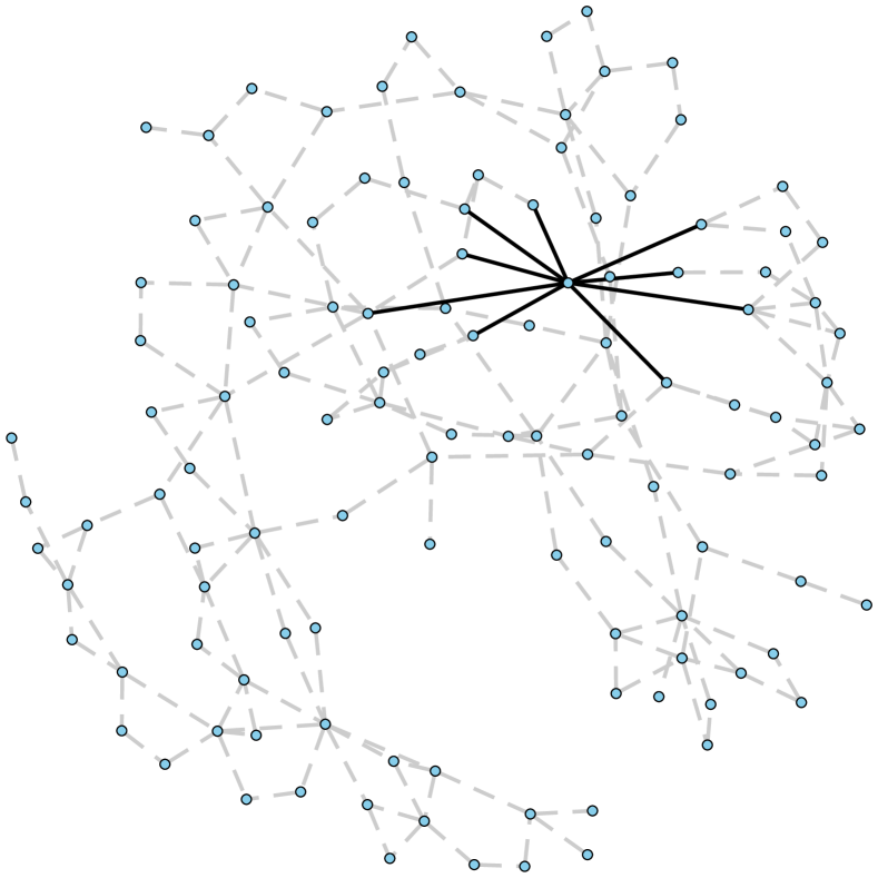
(a) SUD-DBP: $|E(\mathbf{A}^{*})|=9$
$\frac{\lambda^{\prime}}{\mu^{\prime}}=0.0028,\gamma^{\prime}=4.4222$

(b) SUD-DBP: $|E(\mathbf{A}^{*})|=0$
$\frac{\lambda^{\prime}}{\mu^{\prime}}=0.0167,\gamma^{\prime}=1.844$

(c) SUD-DBP: $|E(\mathbf{A}^{*})|=179$
$\frac{\lambda^{\prime}}{\mu^{\prime}}=0.27542,\gamma^{\prime}=28.889$

(d) TRI-DBP: $|E(\mathbf{A}^{*})|=0$
$\frac{\lambda^{\prime}}{\mu^{\prime}}=0.0028,\gamma^{\prime}=4.4222$

(e) TRI-DBP: $|E(\mathbf{A}^{*})|=0$
$\frac{\lambda^{\prime}}{\mu^{\prime}}=0.0167,\gamma^{\prime}=1.844$

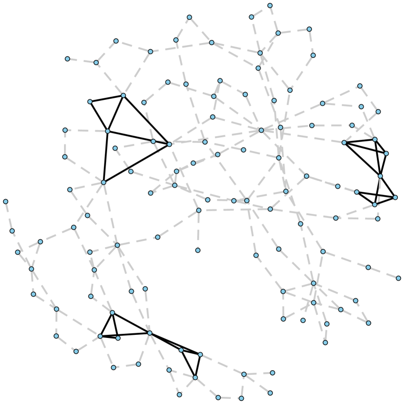
(f) TRI-DBP: $|E(\mathbf{A}^{*})|=28$
$\frac{\lambda^{\prime}}{\mu^{\prime}}=0.27542,\gamma^{\prime}=28.889$

(g) POD-DBP: $|E(\mathbf{A}^{*})|=178$
$\frac{\lambda^{\prime}}{\mu^{\prime}}=0.0028,\gamma^{\prime}=4.4222$

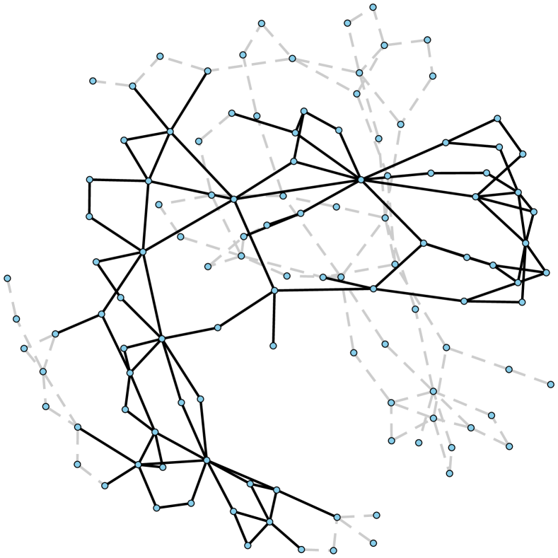
(h) POD-DBP: $|E(\mathbf{A}^{*})|=98$
$\frac{\lambda^{\prime}}{\mu^{\prime}}=0.0167,\gamma^{\prime}=1.844$

(i) SUD-DBP: $|E(\mathbf{A}^{*})|=179$
$\frac{\lambda^{\prime}}{\mu^{\prime}}=0.27542,\gamma^{\prime}=28.889$

Figure 7: 118-bus Test Case Most-Probable Network (solid edges = close, dashed edges = open)

In this section, we use DBP to model cascading failures of transmission lines on the IEEE 118 Bus Test CaseChristie (1993). The network is a portion of the Midwestern US power grid from 1962. It remains one of the standard test cases today. We only use the network topology provided by the test case. The nodes in the network represent the buses and the edges represent transmission lines between the buses. We model edge closures as line failures and edge opening as recovery. During cascading failures like blackouts, transmission line $(a,b)$ is more likely to fail if there are already many failed transmission lines at bus (i.e., node) $a$ and bus $b$. Therefore, it is intuitive to assume that $\gamma^{\prime}>1$. On the other hand, spontaneous failures are rare events and since the power grid is well maintained, the recovery rate of failed transmission lines is relatively high; it is natural to assume that $0<\frac{\lambda^{\prime}}{\mu^{\prime}}\leq 1$.

Figure 7 shows the most-probable network with different dynamic parameters $\lambda^{\prime},\gamma^{\prime},\mu^{\prime}$ for SUD-DBP, TRI-DBP, and POD-DBP. When the closure (i.e., failure) rate of an edge is low compared with the opening rate (i.e., recovery), $\mathbf{A}^{*}=\mathbf{A}_{0}$ as in Regime I). When the closure (i.e., failure) rate of an edge is high compared with the opening rate (i.e., recovery), $\mathbf{A}^{*}=\mathbf{A}_{\max}$ as in Regime IV). However, for a subset of parameters, the most-probable networks are non-degenerate. This means that a subset of edges are more vulnerable to cascading failures than others. We can also see that the contagion dynamic, captured by the cascade function $f(\mathcal{N}_{a},\mathcal{N}_{b})$, has a large impact on the susceptibility of the network to failure.

The dynamics of SUD-DBP (3) put higher probability on network states that minimize the number of closed edges, $|E(\mathbf{A})|$ and maximize the number of induced $P_{3}$ subgraphs. We can see from Figures 7(a), that the most-probable network of SUD-DBP consists of closed edge structures resembling many star subgraphs. Central, hub structures are more vulnerable under SUD-DBP dynamics.

The dynamics of TRI-DBP (4) put high probability on network states that minimize the number of closed edges, $|E(\mathbf{A})|$ but maximize the number of induced $C_{3}$ subgraphs. From Figure 7(f), we can see the the most-probable network consists of triangles. Since the cascade function of TRI-DBP depends on the number of common neighbors, networks with few triangles have the lowest rate of cascading failures.

The dynamics of POD-DBP (5) put high probability on network states that minimize the number of closed edges, $|E(\mathbf{A})|$ but maximize the number of induced $C_{3}$ and $P_{4}$ subgraphs. We can see from Figure 7(h) that the most-probable network consists of more triangles (i.e., $C_{3}$s) and longer paths than the most-probable network of SUD-DBP. POD-DBP has higher rate of cascade than SUD-DBP and TRI-DBP and therefore more lines are vulnerable to cascading failures for the same parameter values.

VI.2 Social Network Example

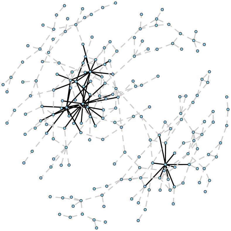
(a) SUD-DBP: $|E(\mathbf{A}^{*})|=54$
$\frac{\lambda^{\prime}}{\mu^{\prime}}=0.0028,\gamma^{\prime}=4.4222$

(b) SUD-DBP: $|E(\mathbf{A}^{*})|=15$
$\frac{\lambda^{\prime}}{\mu^{\prime}}=0.0167,\gamma^{\prime}=1.844$

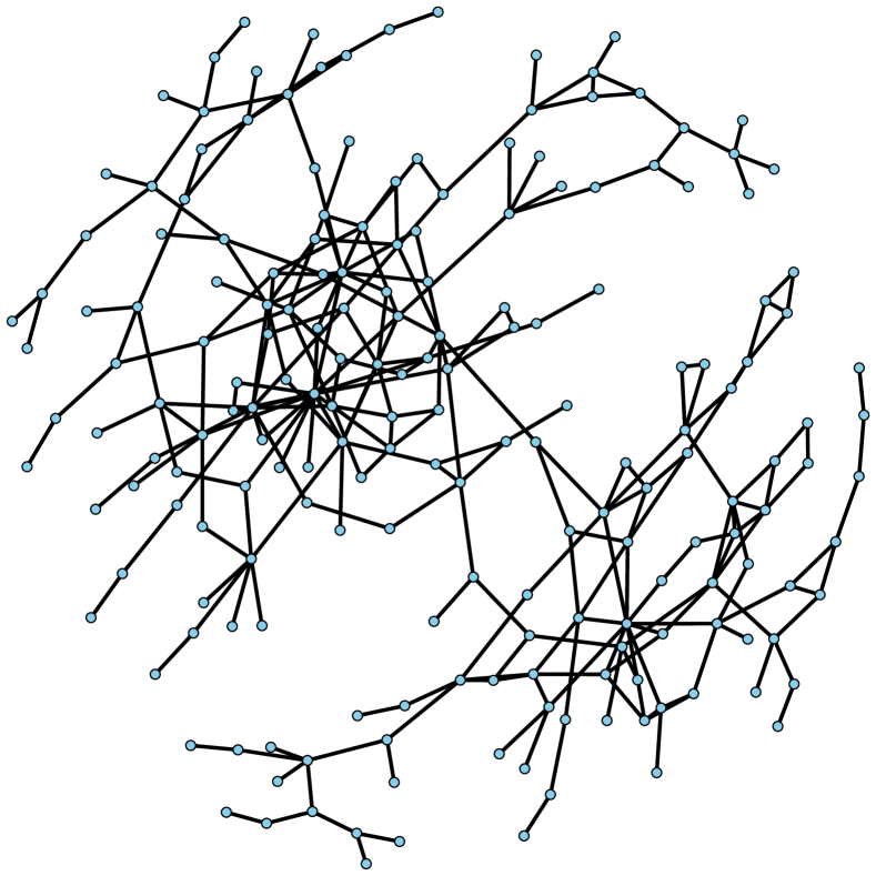
(c) SUD-DBP: $|E(\mathbf{A}^{*})|=273$
$\frac{\lambda^{\prime}}{\mu^{\prime}}=0.27542,\gamma^{\prime}=28.889$

(d) TRI-DBP: $|E(\mathbf{A}^{*})|=0$
$\frac{\lambda^{\prime}}{\mu^{\prime}}=0.0028,\gamma^{\prime}=4.4222$

(e) TRI-DBP: $|E(\mathbf{A}^{*})|=0$
$\frac{\lambda^{\prime}}{\mu^{\prime}}=0.0167,\gamma^{\prime}=1.844$

(f) TRI-DBP: $|E(\mathbf{A}^{*})|=44$
$\frac{\lambda^{\prime}}{\mu^{\prime}}=0.27542,\gamma^{\prime}=28.889$

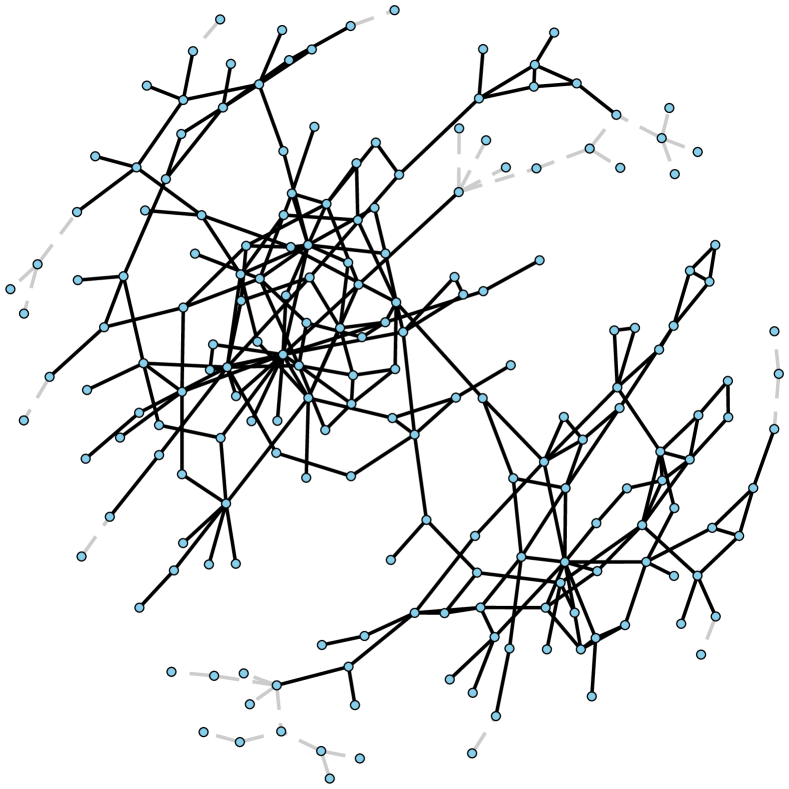
(g) POD-DBP: $|E(\mathbf{A}^{*})|=241$
$\frac{\lambda^{\prime}}{\mu^{\prime}}=0.0028,\gamma^{\prime}=4.4222$

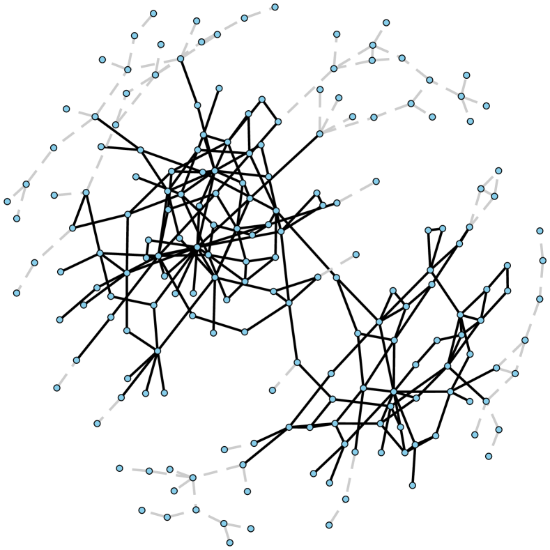
(h) POD-DBP: $|E(\mathbf{A}^{*})|=194$
$\frac{\lambda^{\prime}}{\mu^{\prime}}=0.0167,\gamma^{\prime}=1.844$

(i) POD-DBP: $|E(\mathbf{A})|=273$
$\frac{\lambda^{\prime}}{\mu^{\prime}}=0.27542,\gamma^{\prime}=28.889$

Figure 8: 198-node Social Network Most-Probable Network (solid edges = closed, dashed edges = open)

We also used DBP to model evolving social ties on a 198-node social network of drug users in Hartford, CT Weeks et al. (2002). The nodes in the network represent individual drug users. Edge closure corresponds to formation or reestablishment of social ties, and edge opening corresponds to dissipation of social ties. In this case, edges that are closed in the most-probable networks are the social ties that are often established. They are the stronger social ties between individuals.

Assuming that $\gamma^{\prime}>1$ means that a relationship $(a,b)$ is more likely to form if agent $a$ and agent $b$ already have many other relationships. In particular, TRI-DBP assumes that a relationship $(a,b)$ is more likely to form if agent $a$ and agent $b$ already have many friends in common. This is based on the theory of triadic closure from social networks Brandes et al. (2013). On the other hand, spontaneous friendships are possible and relationships can dissipate over time. Therefore, it is natural to assume nonzero $\lambda^{\prime}$ and $\mu^{\prime}$ and that $0<\frac{\lambda^{\prime}}{\mu^{\prime}}\leq 1$.

Figure 8 shows the most-probable network with different dynamic parameters $\lambda^{\prime},\gamma^{\prime},\mu^{\prime}$ for SUD-DBP, TRI-DBP, and POD-DBP. We can see from Figure 8(f) and Figure 8(h) that, for some range of parameter values, social ties in triadic closures are stronger assuming TRI-DBP and POD-DBP cascade functions. On the other hand, social ties of highly connected individuals are stronger as in SUD-DBP.

VII Regime III) Cascading Prevention

In Regime III) Cascading Prevention: $\frac{\lambda^{\prime}}{\mu^{\prime}}>1$ and $0<\gamma^{\prime}\leq 1$, the structure-free term is driven by edge closure and the structure-dependent term is driven by edge opening. The dynamics of Regime III) Cascading Prevention is the opposite of Regime II) Cascading Failures. The average time an edge is open increases with increasing number of closed edges on its end nodes; diffusion effects, instead of driving cascading failures, preventsedge closures. Therefore, this regime is called Regime III) Cascading Prevention. For SUD-DBP, TRI-DBP, and POD-DBP, we expect the solution space of the Most-Probable Network Problem (18) to exhibit phase transition depending on if edge opening or edge closure dominates.

However, since $0<\gamma^{\prime}\leq 1$ in Regime III), the Most-Probable Network Problem can not be solved using submodularity according to Theorem VI.2. However, we will prove in the next section that we can still solve for the most-probable network in polynomial-time for a sub-range of parameter values in Regime III) for SUD-DBP. In this sub regime, the most-probable network corresponds to the maximum matching (see Definition III.5). For TRI-DBP, the most-probable network corresponds to triangle-free graphs. For POD-DBP, the most-probable network corresponds to the maximum star matching (see Definition III.6).

VII.1 SUD-DBP and Maximum Matching

The dynamics of SUD-DBP in regime III) put high probability on network states that maximize the number of closed edges, $|E(\mathbf{A})|$, and minimize the number of induced $P_{3}$ subgraphs. This means avoiding forming paths of length $2$ and allowing for only paths of length $1$. As a result, for sub-range of parameters, $\frac{\lambda^{\prime}}{\mu^{\prime}},\gamma^{\prime}$, we can prove that the set of close edges in the most-probable network is a maximum matching (see Definition III.5). It is known that the maximum matching can be found in polynomial time for arbitrary, undirected graphs Micali and Vazirani (1980); Harvey (2009). Maximum matching may not be unique.

Theorem VII.1.

In Regime III), if $\lambda^{\prime}\gamma^{\prime}<\mu^{\prime}$, then the most-probable network, $\mathbf{A}^{*}=\{\mathbf{A}\in\mathcal{A}:g(E(\mathbf{A}))=0,|E(\mathbf{A})|\text{ is maximum}\}$, where $g(\mathbf{A})$ is the number of induced $P_{3}$ subgraphs. This is equivalent to stating that $E(\mathbf{A}^{*})$ is a maximum matching (see Definition III.5).

Proof.

We prove the theorem by contradiction. Let $\mathcal{A}^{*}$ denote the set of network states whose set of closed edges are maximum matching.

$$\mathcal{A}^{*}=\{\mathbf{A}\in\mathcal{A}:E(\mathbf{A})\text{ is maximum matching}\}.$$

By the definition of matching, the number of $P_{3}$ subgraphs induced by any network state $\mathbf{A}^{*}\in\mathcal{A}^{*}$, $g(E(\mathbf{A}^{*}))=0$. Suppose that the most-probable network is $\mathbf{A}^{\prime}\in\mathcal{A}\setminus\mathcal{A}^{*}$. Then there are two possibilities for $\mathbf{A}^{\prime}$:

1. $\mathbf{A}^{\prime}$ is the network state such that $E(\mathbf{A}^{\prime})$ is a matching but it is not the maximum matching.

2. $\mathbf{A}^{\prime}$ is the network state such that $E(\mathbf{A}^{\prime})$ is not a matching.

Case 1)

This implies that $|E(\mathbf{A}^{\prime})|<|E(\mathbf{A}^{*})|$ for any $\mathbf{A}^{*}\in\mathcal{A}^{*}$. Since $\frac{\lambda^{\prime}}{\mu^{\prime}}>1$, then by the equilibrium distribution (8), $\pi(\mathbf{A}^{\prime})<\pi(\mathbf{A}^{*})$. Therefore, $\mathbf{A}^{\prime}$ can not be the most-probable network.

Case 2)

This implies that $g(E(\mathbf{A}^{\prime}))>0$. For any $\mathbf{A}^{*}\in\mathcal{A}^{*}$, there are two possibilities

1. $|E(\mathbf{A}^{\prime})|\leq|E(\mathbf{A}^{*})|$
   If $|E(\mathbf{A}^{\prime})|\leq|E(\mathbf{A}^{*})|$, then

   $$\left(\frac{\lambda^{\prime}}{\mu^{\prime}}\right)^{|E(\mathbf{A}^{\prime})|}\gamma^{\prime g(E(\mathbf{A}^{\prime}))}<\left(\frac{\lambda^{\prime}}{\mu^{\prime}}\right)^{|E(\mathbf{A}^{*})|}\gamma^{\prime g(E(\mathbf{A}^{*}))}.$$

   Therefore, $\mathbf{A}^{\prime}$ can not be the most-probable network.

2. $|E(\mathbf{A}^{\prime})|>|E(\mathbf{A}^{*})|$.

   Let $\mathcal{A}^{\prime}_{1}$ denote the set of network states such that for any $\mathbf{A}^{\prime}\in\mathcal{A}^{\prime}_{1}$, $|E(\mathbf{A}^{\prime})|=|E(\mathbf{A}^{*})|+1$. This also implies that the number of $P_{3}$ subgraphs induced by $E(\mathbf{A}^{\prime})$, $g(E(\mathbf{A}))\geq 1$:

   $$\mathcal{A}^{\prime}_{1}=\{\mathbf{A}\in\mathcal{A}:g(E(\mathbf{A}))\geq 1,|E(\mathbf{A})|=|E(\mathbf{A}^{*})|+1\}$$

   Similarly, let $\mathcal{A}^{\prime}_{2}$ denote the set of network states such that for any $\mathbf{A}^{\prime}\in\mathcal{A}^{\prime}_{2}$, $|E(\mathbf{A}^{\prime})|=|E(\mathbf{A}^{*})|+2$:

   $$\mathcal{A}^{\prime}_{2}=\{\mathbf{A}\in\mathcal{A}:g(E(\mathbf{A}))\geq 2,|E(\mathbf{A})|=|E(\mathbf{A}^{*})|+2\}.$$

   We can define additional sets such as $\mathcal{A}^{\prime}_{3}$ $\mathcal{A}^{\prime}_{4},\ldots,\mathcal{A}^{\prime}_{N}$. Realize that $g(E(\mathbf{A}^{\prime}_{2}))>g(E(\mathbf{A}^{\prime}_{1}))$ for any $\mathbf{A}^{\prime}_{1}\in\mathcal{A}^{\prime}_{1}$ and $\mathbf{A}^{\prime}_{2}\in\mathcal{A}^{\prime}_{2}$, $g(E(\mathbf{A}^{\prime}_{3}))>g(E(\mathbf{A}^{\prime}_{2}))$ for any $\mathbf{A}^{\prime}_{2}\in\mathcal{A}^{\prime}_{2}$ and $\mathbf{A}^{\prime}_{3}\in\mathcal{A}^{\prime}_{3}$. Similarly $g(E(\mathbf{A}^{\prime}_{N}))>g(E(\mathbf{A}^{\prime}_{N-1}))$ for any $\mathbf{A}^{\prime}_{N-1}\in\mathcal{A}^{\prime}_{N-1}$ and $\mathbf{A}^{\prime}_{N}\in\mathcal{A}^{\prime}_{N}$.

   Since $0<\gamma^{\prime}\leq 1$, the network state with the maximum equilibrium probability in set $\mathcal{A}^{\prime}_{1}$ has the probability

   $$\pi(\overline{\mathbf{A}^{\prime}_{1}})=\frac{1}{Z}\left(\frac{\lambda^{\prime}}{\mu^{\prime}}\right)^{|E(\mathbf{A}^{*})|+1}\gamma^{\prime}$$

   and the network state with the maximum equilibrium probability in set $\mathcal{A}^{\prime}_{2}$ has the probability

   $$\pi(\overline{\mathbf{A}^{\prime}_{2}})=\frac{1}{Z}\left(\frac{\lambda^{\prime}}{\mu^{\prime}}\right)^{|E(\mathbf{A}^{*})|+2}\gamma^{\prime 2}.$$

   The additional condition $\lambda^{\prime}\gamma^{\prime}<\mu^{\prime}$ implies that $\pi(\overline{\mathbf{A}^{\prime}_{1}})>\pi(\overline{\mathbf{A}^{\prime}_{2}})$. Similar argument will show that $\pi(\overline{\mathbf{A}^{\prime}_{2}})>\pi(\overline{\mathbf{A}^{\prime}_{3}})$, and that $\pi(\mathbf{A}^{\prime}_{N-1})>\pi(\mathbf{A}^{\prime}_{N})$.

   Since

   $$\pi(\mathbf{A}^{*})=\frac{1}{Z}\left(\frac{\lambda^{\prime}}{\mu^{\prime}}\right)^{k},$$

   the network state $\mathbf{A}^{\prime}$ can not be the most-probable network as $\pi(\mathbf{A}^{\prime})\leq\pi(\overline{\mathbf{A}^{\prime}_{1}})$ by definition.

∎

The dynamics of SUD-DBP in regime III) put high probability on network states that maximize the number of closed edges, $|E(\mathbf{A})|$, and minimize the number of induced $P_{3}$ subgraphs. This means avoiding forming paths of length $2$ and allowing for only paths of length $1$. As a result, for a sub-range of parameters, $\frac{\lambda^{\prime}}{\mu^{\prime}},\gamma^{\prime}$, we can prove that the set of close edges in the most-probable network is a maximum matching (see Definition III.5). It is known that the maximum matching can be found in polynomial time for arbitrary, undirected graphs Micali and Vazirani (1980); Harvey (2009). Note that the maximum matching may not be unique.

VII.2 TRI-DBP and Triangle Free Graphs

The dynamics of TRI-DBP in regime III) put higher probability on network states that maximize the number of closed edges, $|E(\mathbf{A})|$ and minimize the number of induced $C_{3}$ subgraphs. This means avoiding forming cycles of length $3$ (i.e., triangles). Consequently, the most-probable configuration will be biased toward the set of closed edges that induces triangle-free graphs.

Theorem VII.2.

In Regime III), if $\lambda^{\prime}\gamma^{\prime}<\mu^{\prime}$, then the most-probable network, $\mathbf{A}^{*}=\{\mathbf{A}\in\mathcal{A}:g(E(\mathbf{A}))=0,|E(\mathbf{A})|\text{ is maximum}\}$, where $g(\mathbf{A})$ is the number of induced $C_{3}$ subgraphs. This is equivalent to stating that $\mathbf{A}^{*}$ is the largest possible triangle-free subgraph in the maximal network.

The proof follows the same argument as in Theorem VII.1.

VII.3 POD-DBP and Maximum Star Matching

The dynamics of POD-DBP in regime III) put higher probability on network states that maximize the number of closed edges, $|E(\mathbf{A})|$ and minimize the number of induced $C_{3}$ and $P_{4}$ subgraphs. This means avoiding forming paths of length $3$ and cycles of length $3$ and allowing paths of length $1$ and $2$. Consequently, the most-probable configuration will be biased toward the set of closed edges that maximizes the number of induced paths of length 2.

Theorem VII.3.

In Regime III), if $\lambda^{\prime}\gamma^{\prime}<\mu^{\prime}$, then the most-probable network, $\mathbf{A}^{*}=\{\mathbf{A}\in\mathcal{A}:g(E(\mathbf{A}))=0,|E(\mathbf{A})|\text{ is maximum}\}$, where $g(\mathbf{A})$ is the number of induced $C_{3}$ and $P_{4}$ subgraphs. This is equivalent to stating that $E(\mathbf{A}^{*})$ is a maximum star matching (see Definition III.6).

The proof follows the same argument as in Theorem VII.1.

VIII Conclusion

We presented the Dynamic Bond Percolation process, a stochastic, edge-centric network process. DBP assumed that an edge in the maximal network can spontaneously open or close. In addition, the closure rate of an edge also depends on the state of the neighboring edges. This is captured by the cascade function, $f(\mathcal{N}_{a},\mathcal{N}_{b})$. In this paper, we considered 3 different variations of DBP: 1) SUD-DBP, 2) TRI-DBP, and 3) POD-DBP. The advantage of DBP over other existing network process models is that the equilibrium distribution can be derived in closed-form for arbitrary maximal network.

We proved that the sufficient statistics of SUD-DBP at equilibrium are the number of closed edges, $|E(\mathbf{A})|$, and the number of $P_{3}$ subgraphs. The sufficient statistics of TRI-DBP are the number of closed edges, $|E(\mathbf{A})|$, and the number of $C_{3}$ subgraphs. The sufficient statistic of POD-DBP are the number of closed edges, $|E(\mathbf{A})|$, and the number of $C_{3}$ and $P_{4}$ subgraphs. As the sufficient statistics are different depending on the cascade function, it is intuitive that the most-probable network of the process may also differ.

In Regime I) Recovery Dominant and Regime IV) Removal Dominant, this is not the case since SUD-DBP, TRI-DBP, and POD-DBP all lead to the consensus most-probable network of $\mathbf{A}_{0}$ and $\mathbf{A_{\max}}$. This does not apply to Regime II) Cascading Failures and Regime III) Cascading Prevention. We proved that the Most-Probable Configuration Problem can be solved using polynomial-time algorithm in Regime II) because solving the optimization of the most-probable configuration corresponds to finding the minimum of a submodular function. We illustrated using two real-world, heterogenous networks, phase transition behavior as well as the existence of non-degenerate solutions of the Most-Probable Configuration Problem. This means that, for certain processes, some subset of edges is more critical than others. In SUD-DBP, these at-risk edges tend to belong to edges in large star subgraphs; in POD-DBP and TRI-DBP, they tend to belong to edges in triangle subgraphs.

In Regime III), we proved that, for a subregime of parameters, the solution of the Most-Probable Network Problem corresponds to maximum matching for SUD-DBP. For TRI-DBP, the solution corresponds to triangle-free graphs. For POD-DBP, the solution corresponds to maximum star matching. We showed with DBP and preliminary analysis that the underlying topology and the form of the cascade function have a large impact on the equilibrium behavior of the dynamical process. In the future, we will extend our analysis to transient behaviors as well as considering other cascade functions.

Appendix A Determining $g(E(\mathbf{A}))$ for SUD-DBP

For the Sum-Dependent Dynamic Bond Percolation Model, $g(E(\mathbf{A}))$ is the number of paths of length 2 formed by the set of edges, $E(\mathbf{A})$, of the network represented by the adjacency matrix $\mathbf{A}$. The number of walks of length 2 from node $i$ to node $j\neq i$ is

$$\sum_{i=1}^{N}\sum_{j>i}(\mathbf{A}^{2})_{i,j}.$$

Realize that this is also equivalent to the number of paths of length 2 from node $i$ to node $j\neq i$.

Appendix B Determining $g(E(\mathbf{A}))$ for POD-DBP

For the Product-Dependent Dynamic Bond Percolation Model, $g(E(\mathbf{A}))$ is the number of triangles and of paths of length 3 formed by the set of edges, $E(\mathbf{A})$, of the network represented by the adjacency matrix $\mathbf{A}$. The number of cycles of length $3$ is

$$\sum_{i=1}^{N}\frac{(\mathbf{A}^{3})_{i,i}}{6}.$$

We need to find the number of paths of length 3. We know that the number of walks of length 3 from node $i$ to node $j\neq i$ is

$$\sum_{i=1}^{N}\sum_{j>i}(\mathbf{A}^{3})_{i,j}.$$

This number is larger than the number of paths of length 3 because there are walks from node $i$ to node $j$ that are not paths. Figure 9 illustrates the three cases of walks of length 3 that are not paths of length 3 because the vertices repeat.

(a) Walk of Length 3 from Node $i$ to Node $j$: $i,e_{1},k,e_{2},i,e_{3},j$

(b) Walk of Length 3 from Node $i$ to Node $j$: $i,e_{1},j,e_{2},k,e_{3},j$

(c) Walk of Length 3 from Node $i$ to Node $j$: $i,e_{1},k,e_{2},i,e_{3},j$

Figure 9: Walks of Length 3 that are not Paths of Length 3

Therefore, the number of paths of length 3 from node $i$ to node $j\neq i$ is

$$\begin{split}&\sum_{i=1}^{N}\sum_{j>i}(\mathbf{A}^{3})_{i,j}-(\mathbf{A}_{i,j})\sum_{k=1,k\neq i,j}^{N}\mathbf{A}_{i,k}-(\mathbf{A}_{i,j})\sum_{k=1,k\neq i,j}^{N}\mathbf{A}_{j,k}-\mathbf{A}_{i,j}\\ =&\sum_{i=1}^{N}\sum_{j>i}(\mathbf{A}^{3})_{i,j}-(\mathbf{A}_{i,j})\left(\sum_{k=1,k\neq i,j}^{N}\mathbf{A}_{i,k}+\sum_{k=1,k\neq i,j}^{N}\mathbf{A}_{j,k}+1\right)\\ =&\sum_{i=1}^{N}\sum_{j>i}(\mathbf{A}^{3})_{i,j}-(\mathbf{A}_{i,j})\left((\mathbf{A}^{2})_{i,i}+\sum_{k=1,k\neq i,j}^{N}\mathbf{A}_{k,j}\right).\end{split}$$ (24)

This leads to

$$\begin{split}&g(E(\mathbf{A}))=\sum_{i=1}^{N}\frac{(\mathbf{A}^{3})_{i,i}}{6}+\\ &\sum_{i=1}^{N}\sum_{j>i}(\mathbf{A}^{3})_{i,j}-(\mathbf{A}_{i,j})\left((\mathbf{A}^{2})_{i,i}+\sum_{k=1,k\neq i,j}^{N}\mathbf{A}_{k,j}\right).\end{split}$$

References

- Minkel [2008] J.R. Minkel. The 2003 northeast blackout–five years later. Scientific American, 13, 2008.
- Jackson [2008] M. O. Jackson. Social and Economic Networks. Princeton University Press, 2008.
- Newman [2010] Mark Newman. Networks: an Introduction. Oxford University Press, 2010.
- Eames and Keeling [2002] Ken T.D. Eames and Matt J. Keeling. Modeling dynamic and network heterogeneities in the spread of sexually transmitted diseases. Proceedings of the National Academy of Sciences, 99(20):13330–13335, 2002.
- Zhang and Moura [2014] June Zhang and José M. F. Moura. Diffusion in social networks as SIS epidemics: Beyond full mixing and complete graphs. IEEE Journal of Selected Topics in Signal Processing, 8(4):537–551, Aug 2014. doi: 10.1109/JSTSP.2014.2314858.
- Zhang and Moura [2015] June Zhang and José M. F. Moura. Role of subgraphs in epidemics over finite-size networks under the scaled SIS process. Journal of Complex Networks, 2015. doi: 10.1093/comnet/cnv006.
- Wasserman [1980] Stanley Wasserman. Analyzing social networks as stochastic processes. Journal of the American Statistical Association, 75(370):280–294, 1980.
- Leenders [1995] Roger Th. A.J. Leenders. Models for network dynamics: A Markovian framework. Journal of Mathematical Sociology, 20(1):1–21, 1995.
- Snijders [2005] Tom AB Snijders. Models for longitudinal network data. Models and Methods in Social Network Analysis, 1:215–247, 2005.
- Pepyne [2007] David L Pepyne. Topology and cascading line outages in power grids. Journal of Systems Science and Systems Engineering, 16(2):202–221, 2007.
- Granovetter [1973] Mark S Granovetter. The strength of weak ties. American Journal of Sociology, pages 1360–1380, 1973.
- Broadbent and Hammersley [1957] Simon R Broadbent and John M Hammersley. Percolation processes. In Mathematical Proceedings of the Cambridge Philosophical Society, volume 53, pages 629–641. Cambridge University Press, 1957.
- Callaway et al. [2000] Duncan S Callaway, Mark EJ Newman, Steven H Strogatz, and Duncan J Watts. Network robustness and fragility: percolation on random graphs. Physical Review Letters, 85(25):5468, 2000.
- Steif [2009] Jeffrey E Steif. A survey of dynamical percolation. In Fractal Geometry and Stochastics IV, pages 145–174. Springer, 2009.
- Liggett [1999] Thomas M Liggett. Stochastic Interacting Systems: Contact, Voter and Exclusion Processes, volume 324. Springer, 1999.
- Barrat et al. [2008] Alain Barrat, Marc Barthelemy, and Alessandro Vespignani. Dynamical Processes on Complex Networks, volume 1. Cambridge University Press Cambridge, 2008.
- Christie [1993] Rich Christie. Power system test archive, May 1993. URL https://www.ee.washington.edu/research/pstca/pf118/pg_tca118bus.htm.
- Weeks et al. [2002] Margaret R Weeks, Scott Clair, Stephen P Borgatti, Kim Radda, and Jean J Schensul. Social networks of drug users in high-risk sites: finding the connections. AIDS and Behavior, 6(2):193–206, 2002.
- Brandes et al. [2013] Ulrik Brandes, Jürgen Pfeffer, and Ines Mergel. Studying social networks: A guide to empirical research. Campus, 2013.
- Kelly [1979] F.P. Kelly. Reversibility and Stochastic Networks, volume 40. Wiley New York, 1979.
- Norris [1998] James R Norris. Markov Chains. Cambridge University Press, 1998.
- West [1996] Douglas B West. Introduction to Graph Theory. Prentice Hall, 1996.
- Boros and Hammer [2002] Endre Boros and Peter L Hammer. Pseudo-boolean optimization. Discrete Applied Mathematics, 123(1):155–225, 2002.
- Grötschel et al. [1981] Martin Grötschel, László Lovász, and Alexander Schrijver. The ellipsoid method and its consequences in combinatorial optimization. Combinatorica, 1(2):169–197, 1981.
- Billionnet and Minoux [1985] A Billionnet and M Minoux. Maximizing a supermodular pseudoBoolean function: A polynomial algorithm for supermodular cubic functions. Discrete Applied Mathematics, 12(1):1–11, 1985.
- Schrijver [2003] Alexander Schrijver. Combinatorial Optimization: Polyhedra and Efficiency, volume 24. Springer Science & Business Media, 2003.
- Micali and Vazirani [1980] Silvio Micali and Vijay V Vazirani. An O algoithm for finding maximum matching in general graphs. In 21st Annual Symposium on Foundations of Computer Science, pages 17–27. IEEE, 1980.
- Harvey [2009] Nicholas JA Harvey. Algebraic algorithms for matching and matroid problems. SIAM Journal on Computing, 39(2):679–702, 2009.