Muon Identification with Muon Telescope Detector at the STAR Experiment

Abstract

The Muon Telescope Detector (MTD) is a newly installed detector in the STAR experiment. It provides an excellent opportunity to study heavy quarkonium physics using the dimuon channel in heavy ion collisions. In this paper, we report the muon identification performance for the MTD using proton-proton collisions at $\sqrt{s}$ = 500 GeV with various methods. The result using the Likelihood Ratio method shows that the muon identification efficiency can reach up to $\sim$90% for muons with transverse momenta greater than 3 GeV/c and the significance of the $J/\psi$ signal is improved by a factor of 2 compared to using the basic selection.

1 Introduction

The Solenoidal Tracker At RHIC (STAR) [1] is one of the two large high energy nuclear physics experiments at the Relativistic Heavy Ion Collider (RHIC) at Brookhaven National Laboratory. After 15 years of operation, the STAR experiment has provided many important results, which have helped to improve our understanding of Quantum Chromodynamics (QCD). In particular, evidence of the existence of the Quark Gluon Plasma (QGP) opened a new window to get a deeper insight into QCD [2]. Heavy quarkonia states are ideal probes to study the properties of QCD matter. For instance, quarkonium suppression in the medium due to the color-screening of surrounding partons can provide information about the partonic nature of the QGP and its temperature [3, 4]. Quarkonia are identified by reconstructing their invariant mass ($M_{inv.}$) in the dilepton decay channel. Muons can be reconstructed more precisely due to their reduced bremsstrahlung radiation in material compared to electrons. A new subdetector in STAR, the Muon Telescope Detector (MTD), dedicated to measuring muons was proposed in 2009 and was installed from 2012 to 2014 [5, 6]. In this paper, we present the muon identification performance of this new detector. There have been many studies on muon identification from different experiments, and more details can be found in Refs. [7, 8, 9].

This paper is arranged as follows. In Section 2, a brief description of the STAR detector is presented. The data sets and event selection are described in Section 3. In Section 4, three methods used to identify muon candidates are described. We present in section 5 the efficiency as well as the resulting signal significance for $J/\psi$ from these three methods. Finally, a summary is given in Section 6.

2 The STAR detector

The STAR detector is a general purpose particle detector optimized for high energy nuclear physics. The main subsystems relevant to this analysis include the Time Projection Chamber (TPC), the Magnet System and the MTD. The TPC is the primary tracking detector for charged particles and provides particle identification via measurements of the energy loss ($dE/dx$) [10]. It covers full azimuthal angles ($0<\phi<2\pi$) and a large pseudorapidity range ($|\eta|<1$). The transverse momenta ($p_{T}$) and charge (q) of charged particles are measured by the curvature of their trajectories in the 0.5 Tesla solenoidal field generated by the Magnet System. There are 30 bars, known as “backlegs”, outside the coil to provide the return flux path for the magnetic field [11]. They are 61 cm thick at a radius of 363 cm corresponding to about 5 absorption lengths. These backlegs play an essential role in enhancing the muon purity by absorbing the background hadrons from collisions. The MTD is a fast detector based on the Multi-gap Resistive Plate Chamber technology to record signals, also referred to as signals (“hits”) generated by charged particles traversing it. It provides single-muon and dimuon triggers based on the number of hits within a predefined online timing window. The MTD modules are installed at a radius of about 403 cm, and cover about 45% in azimuth within $|\eta|<$ 0.5 [5]. Installation of the full MTD was 10%, 63%, and 100% completed for the 2012, 2013, and 2014 run years respectively. As shown in cosmic ray data, the timing resolution of the MTD is $\sim$100 ps and the spatial resolutions are $\sim$1-2 cm in both $r\phi$ and $z$ directions [12].

3 Dataset and event selection

3.1 Data and Monte Carlo

Data for this study were collected by the STAR detector during the RHIC proton-proton run at a center of mass energy of 500 GeV in 2013. Events in the data sample were selected using the MTD dimuon trigger which requires at least two MTD hits in coincidence with the bunch crossing. The data set represents an integrated luminosity of 28.3 pb^-1.

The detector response to the $J/\psi\to\mu^{+}\mu^{-}$ signal was studied using a Monte Carlo (MC) simulation. The MC sample was generated by a single-particle generator with flat distribution in $p_{T}$, $\phi$ and $\eta$ for $J/\psi$. These simulated signals were then passed through the full GEANT3 [13] simulation of the STAR detector, and “embedded” into real events, followed by the standard reconstruction procedure as used for real data. The kinematic distributions of the embedded $J/\psi$ and $\mu^{\pm}$ were weighted by the $p_{T}$ spectrum of $J/\psi$ in $pp$ collisions at 500 GeV determined via interpolation through a global fit of world-wide differential $J/\psi$ cross section measurements [14]. The reconstructed muon $p_{T}$ in MC was also slightly smeared by a Gaussian function, with mean = $1.004\times p_{T}$ and width = $0.022\times p_{T}$, to match the reconstructed $J/\psi$ mass distribution in data.

3.2 Track selection

Tracks selected for the muon identification study have to meet the following requirements: $p_{T}$ is greater than 1 GeV/c; the distance of closest approach to the collision vertex should be less than 3 cm to suppress secondary decays; number of TPC clusters used in reconstruction should be greater than 15 (the maximum possible is 45) to have good momentum resolution; number of TPC clusters used for the $dE/dx$ measurement is greater than 10 to ensure good $dE/dx$ resolution; the ratio of the number of used TPC clusters over the number of possible clusters is not less than 0.52 in order to reject split tracks. Tracks are also required to project to MTD hits that fire the triggers.

Figure 1 shows the invariant mass spectrum of opposite-sign dimuon pairs with the selection criteria described above applied to both candidate daughters. The $J/\psi$ signal is clear around 3.1 GeV/c². More than 1500 $J/\psi$ candidates are present in the data sample used here. Lighter mesons, like $\omega$, $\phi$ and $\eta$ particles particles are obscured by large backgrounds at low $M_{inv.}$.

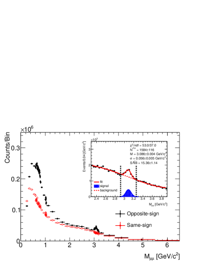
Figure 1: The dimuon mass spectrum with basic selection described in Section 3.2 applied to both muons. The black solid and red open circles are for the muon pairs with opposite and same signs in charge, respectively. The inset shows the dimuon mass fits for $J/\psi$ peak. The solid red line is a combined fit to the signal and background with a single Gaussian plus a fourth-order polynomial, and the two vertical black dashed lines indicate the mass window [2.92 - 3.25 GeV/c²] used to select the $J/\psi$ candidates.

4 Muon identification

4.1 Methods

To distinguish muon candidates from the hadron background, there are four variables, $\Delta$ToF, $\Delta y\times q$, $\Delta z$ and $n\sigma_{\pi}$ used in this study. $\Delta$ToF is the difference between the calculated time-of-flight value from track extrapolation with a muon particle hypothesis and the measured one from the MTD detector. $\Delta z$ and $\Delta y$ are the residuals between the MTD hit position and extrapolated track position on the MTD, where $z$ is along the beam pipe and $y$ is perpendicular to z along the surface of each MTD module (approximately $r\phi$). $\Delta y$ is multiplied by charge ($\Delta y\times q$) to eliminate the charge dependence. $n\sigma_{\pi}$ is the difference between the measured $dE/dx$ and the theoretical value assuming the track is a pion (for simplicity with pre-existing codes), normalized to the $dE/dx$ resolution of the TPC:

$$n\sigma_{\pi}=\frac{(\log\frac{dE}{dx})_{{\rm measured}}-(\log\frac{dE}{dx})_{\pi,{\rm theory}}}{\sigma(\log\frac{dE}{dx})_{{\rm measured}}}.$$ (1)

The probability distribution functions (PDFs) of each variable for same sign dimuon pairs (SS) within the $M_{inv.}$ window [2.92, 3.25] GeV/c² (shown by vertical dashed black lines in the inset of Fig. 1) were used to characterize backgrounds. The PDFs of pure muons were then obtained by a subtraction of the background PDFs from those of opposite sign dimuon pairs (OS) within the same $M_{inv.}$ window. Similar distributions are extracted from MC as well except for the $\Delta$ToF distribution because the timing signal of MTD is not modeled in the simulation. Figure 2 shows the comparisons for the PDF of each variable between signal (data and MC) and background. The signal distributions in data and MC are in reasonable agreement.

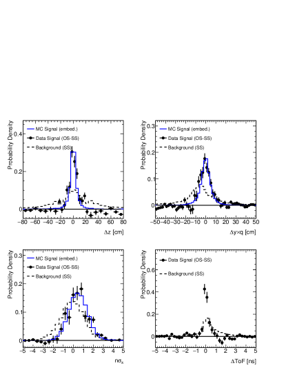
Figure 2: The probability density function of $\Delta$z, $\Delta y\times q$, $\Delta$ToF, and $n\sigma_{\pi}$ variables. The black points are the signal from data (OS-SS), the solid line histograms are the signal from MC, and the dashed line histograms are the background from data (SS).

Three methods, straight cut, N-1 iteration and Likelihood Ratio, are utilized in this paper to identify muon candidates. The performance of these three methods is quantified using a tag-and-probe procedure. In the low muon $p_{T}$ region ($p_{T}<3.5$ GeV/c), the tagged muon is the one with higher $p_{T}$, while the probed muon is the one with lower $p_{T}$. However, in the high muon $p_{T}$ region ($p_{T}>3.5$ GeV/c), in contrast, the tagged (probed) muon is the one with lower (higher) $p_{T}$ to increase statistics. The muon identification cuts are applied on the probed muons, and then the efficiency and background rejection power can be obtained by comparing the yield and significance of the $J/\psi$ signal from before and after the selection. Several signal (single Gaussian or Crystal-Ball function) and background (third-order or fourth-order polynomial function) models are used to fit the dimuon mass spectra. The efficiency is calculated by using the average fitted values for the number of $J/\psi$ from all combinations of signal and background models, and the fit model uncertainty is determined by using the maximum deviation of any fit result from the average.

• Straight cut method
  The simplest way to reduce background is to directly apply cuts on these four variables. An about $\pm 2.5\sigma$ window cut on $\Delta z$ and $\Delta y\times q$, and an asymmetric window cut, $-1.5\sigma$ to $+2.5\sigma$, on $n\sigma_{\pi}$ are used to retain high efficiency while rejecting background, where $\sigma$ is the width of the signal distributions as shown in Fig. 2. An empirical asymmetric cut is used for $\Delta{\rm ToF}$ since the hadron background has a long tail to the right. Specifically, the selection criteria are $-5<\Delta{\rm ToF}<0.2$ ns, $|\Delta z|<20$ cm, $|\Delta y\times q|<20$ cm and $-1<n\sigma_{\pi}<3$.

• N-1 iteration method
  An advanced way to select muon candidates, called N-1 iteration, is to vary one variable to optimize the $J/\psi$ signal significance ($S/\sqrt{B}$) with the other N-1 variables fixed at each iteration step. The values of the cuts determined using this method are $-4.8<\Delta{\rm ToF}<0.7$ ns, $-15<\Delta z<19$ cm, $-9<\Delta y\times q<14$ cm and $-0.5<n\sigma_{\pi}<3.6$.

• Likelihood Ratio method
  A more sophisticated way to reduce the background level and keep high purity simultaneously is using more powerful multivariate methods, such as the Likelihood Ratio method. The basic idea is to create a discriminative variable in the form of a likelihood ratio $R=(1-Y)/(1+Y)$, where $Y=\prod y_{i}$ and each $y_{i}=PDF^{\rm bkg}_{i}/PDF^{\rm sig}_{i}$ is a ratio between background and signal PDFs. Due to the limited statistics in data for the signal PDFs which causes large fluctuations, the embedded MC sample is used to construct the signal PDFs. In this method, only three variables, $\Delta y\times q$, $\Delta z$ and $n\sigma_{\pi}$, are used to calculate the $R$ value for the probed muon. The cut values on $\Delta$ToF are fixed from the N-1 iteration method. Figure 3 shows the PDF ratios ($PDF^{bkgd}/PDF^{sig}$) for, $\Delta y\times q$, $\Delta z$, and $n\sigma_{\pi}$, respectively. A bin-to-bin interpolation (solid red line) is used to obtain the ratios between points in the middle region while a linear fit (dashed red line) is used for the side regions where statistics are low. Figure 4 shows the discriminating power of the Likelihood Ratio method, and the cut value on $R$ variable, $R>-0.2$, is chosen to maximize the significance of the $J/\psi$ signal as shown in Fig. 4.

  

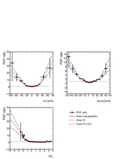
  Figure 3: The PDF ratios of $\Delta$z, $\Delta y\times q$, $\Delta$ToF, and $n\sigma_{\pi}$ variables. The solid red line indicates the bin-to-bin interpolation and the dashed red line is a linear fit to parameterize the ratio.

  

  

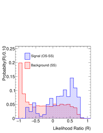
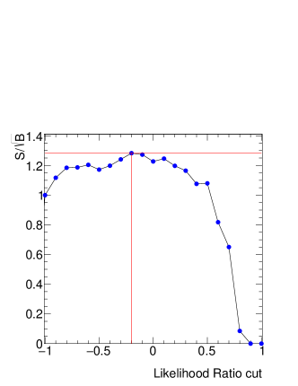
  Figure 4: 4 Distributions of the Likelihood Ratio (R) for signal (blue) and background (red). 4 The cut value on R variable is optimized using the signal significance.

4.2 Systematic uncertainties

The following sources of systematic uncertainty on the muon identification efficiency are considered for these three methods: the background and signal fit models used in data, and the smearing on muon $p_{T}$ in MC. For the Likelihood Ratio method, different methods to build the PDF ratios and different procedures to extract the ratios are also considered. The systematic uncertainties from using different fit models, as described in Section 4.1, are about 5 - 7% in data. The $p_{T}$ smearing uncertainty in MC is evaluated by varying the mean and width in the smearing function to match the mean and width of reconstructed $J/\psi$ mass within $\pm 1\sigma$. In addition, for the Likelihood Ratio method, we compared the results from using sideband or same-sign data as the background PDFs, from extracting the ratios in the middle region via bin-to-bin interpolation or via fitting with a third-order polynomial function, and from varying the fit function by $\pm 1\sigma$ in the side region shown as the blue dot-dashed lines in Fig. 3. The maximum deviation from the average of these results is assigned as the uncertainty related to determining the PDF ratios. The total systematic uncertainties in different $p_{T}$ bins are 0.9 - 8.7% (0.6 - 2.6%), 0.9 - 10.5% (0.2 - 2.1%) and 0.6 - 15.4% (0.5 - 3.8%) for straight cuts, N-1 iteration and Likelihood Ratio method in data (MC), respectively.

5 Results

The performances of different muon identification methods are evaluated by using $J/\psi\to\mu^{+}\mu^{-}$ signals with the selection cuts applied on the probed (subleading) muons as shown in Fig. 5. All of them have the capability to reduce the background level by more than 65% while keeping the $J/\psi$ efficiency relatively high. The muon identification efficiencies are calculated relative to the basic selection described in Section 3.2, and shown as a function of $p_{T}$ in Fig. 6. The plateau efficiency ($p_{T}>$ 3 GeV) is about 90% for the Likelihood Ratio method, and about 80% for the other methods. For the $J/\psi$ signal, the Likelihood Ratio method provides an overall efficiency of about 80% and improves the significance by a factor of 1.38. Detailed comparisons between all three methods are summarized in Table 1.

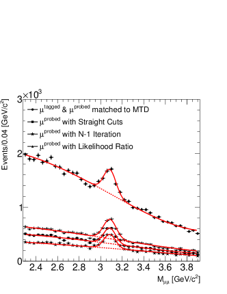
Figure 5: The dimuon mass spectra with various muon identification methods. The solid curves are combined fits to the mass distribution with a Gaussian distribution plus a fourth-order polynomial function. The dashed lines show the fitted background. The solid circles are for the basic selection applied to both muons; the open boxes, open circles and solid triangles are for the cases that the subleading muon is selected using straight cut, N-1 iteration cut and the Likelihood Ratio methods, respectively.

	Basic selection	Straight cut	N-1 iteration	Likelihood Ratio
Signal	1656 $\pm$ 143 $\pm$ 114	1006 $\pm$ 67 $\pm$ 20	891 $\pm$ 58 $\pm$ 12	1346 $\pm$ 74 $\pm$ 22
Background	10861 $\pm$ 104 $\pm$ 317	2682 $\pm$ 52 $\pm$ 80	1962 $\pm$ 44 $\pm$ 58	3743 $\pm$ 61 $\pm$ 79
$S/B$	0.15 $\pm$ 0.01 $\pm$ 0.01	0.38 $\pm$ 0.03 $\pm$ 0.01	0.45 $\pm$ 0.03 $\pm$ 0.01	0.36 $\pm$ 0.02 $\pm$ 0.01
$S/\sqrt{B}$	15.89 $\pm$ 1.37 $\pm$ 1.12	19.44 $\pm$ 1.31 $\pm$ 0.49	20.11 $\pm$ 1.33 $\pm$ 0.39	22.01 $\pm$ 1.23 $\pm$ 0.43
$\varepsilon_{signal}$	—	0.61 $\pm$ 0.01 $\pm$ 0.05	0.54 $\pm$ 0.01 $\pm$ 0.05	0.81 $\pm$ 0.01 $\pm$ 0.07
$1-\varepsilon_{bkgd.}$	—	0.75 $\pm$ 0.01 $\pm$ 0.02	0.82 $\pm$ 0.01 $\pm$ 0.01	0.66 $\pm$ 0.01 $\pm$ 0.01
$\varepsilon_{signal}^{MC}$	—	0.62 $\pm$ 0.01 $\pm$ 0.03	0.51 $\pm$ 0.01 $\pm$ 0.03	0.80 $\pm$ 0.01 $\pm$ 0.04

Table 1: Comparison of the performance for three muon identification methods. $\varepsilon_{signal}$ and $1-\varepsilon_{bkgd.}$ are the muon identification efficiency and the background rejection rate relative to the basic selection, respectively. The first and second errors are the statistical and systematic uncertainties, respectively.

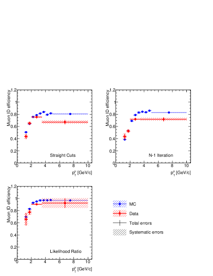
Figure 6: The muon identification efficiencies as a function of $p_{T}$ with straight cuts, N-1 iteration and Likelihood Ratio methods. The blue solid points are from MC, while the red open circles are from data. The error bars are the total uncertainties (statistical plus systematic), while the shaded boxes represent the systematic uncertainties.

After applying the muon identification selections determined using the Likelihood Ratio method on both muons, not only the significance of the $J/\psi$ signal is enhanced by a factor of 2 ($S/\sqrt{B}=31.89$), but also the peaks of the light mesons, such as $\rho$, $\omega$ and $\phi$, become clearer as shown in Fig. 7. This offers a good opportunity to study light mesons, heavy quarkonium, and the dimuon continuum at the STAR experiment.

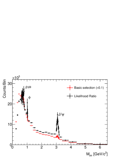
Figure 7: The dimuon mass spectrum with both muons selected with Likelihood Ratio method compared with that using basic selection which is scaled by 0.1. The significance of $J/\psi$ signal is greatly enhanced and the light mesons are clearly visible.

6 Conclusion

The MTD is a newly installed detector dedicated to triggering on and identifying muons in STAR with low kinematic cutoff. In this paper, we evaluated three different muon identification methods: straight cut, N-1 iteration and Likelihood Ratio method. Each of these can reduce the background level by more than 65% and keep the $J/\psi$ signals with about 60% of efficiency. With this muon identification capability, the MTD opens the door to study heavy-ion physics with muons, especially the quarkonium states, in the STAR experiment.

7 Acknowledgments

We thank the STAR Collaboration, the RACF at BNL and National Cheng Kung University (Taiwan) for their support. This work was supported in part by the U.S. DOE Office of Science under the contract No. de-sc0012704 and the Goldhaber Fellowship program at Brookhaven National Laboratory. L. Ruan acknowledges a DOE Office of Science Early Career Award. We thank Dr. Gene Van Buren (BNL) for the proofreading.

References

References

- [1] K. H. Ackermann et al. (STAR Collaboration) , Nucl. Instr. and Meth. A 499 (2003), 624.
- [2] M. Gyulassy, arXiv:nucl-th/0403032 (2004).
- [3] T. Matsui, H. Satz, Phys. Lett. B 178 (1986), 416.
- [4] A. Mocsy, Eur. Phys. J. C 61 (2009), 705.
- [5] L. Ruan et al, J. Phys G 36 (2009), 095001.
- [6] Z. Xu, BNL LDRD project 07-007; Beam Test Experiment (T963) at FermiLab.
- [7] ATLAS Collaboration, Eur. Phys. J. C 74 (2014), 3130.
- [8] The CMS Collaboration, J. of Instr. 7 (2012), 10.
- [9] LHCb Collaboration, J. of Instr. 10 (2013), 10.
- [10] M. Anderson et al. (STAR Collaboration), Nucl. Instr. and Meth. A 499 (2003), 659.
- [11] F. Bergsma et al. (STAR Collaboration), Nucl. Instr. and Meth. A 499 (2003), 633.
- [12] C. Yang et al, Nucl. Instr. and Meth. A762 (2014), 1-6.
- [13] CERN Program Library Long Writeup W5013.
- [14] W. Zha et al., arXiv:1506.08985 (2015).