Asteroid models from the Lowell Photometric Database

Abstract

Context. Information about shapes and spin states of individual asteroids is important for the study of the whole asteroid population. For asteroids from the main belt, most of the shape models available now have been reconstructed from disk-integrated photometry by the lightcurve inversion method.

Aims. We want to significantly enlarge the current sample ($\sim$ 350) of available asteroid models.

Methods. We use the lightcurve inversion method to derive new shape models and spin states of asteroids from the sparse-in-time photometry compiled in the Lowell Photometric Database. To speed up the time-consuming process of scanning the period parameter space through the use of convex shape models, we use the distributed computing project Asteroids@home, running on the Berkeley Open Infrastructure for Network Computing (BOINC) platform. This way, the period-search interval is divided into hundreds of smaller intervals. These intervals are scanned separately by different volunteers and then joined together. We also use an alternative, faster, approach when searching the best-fit period by using a model of triaxial ellipsoid. By this, we can independently confirm periods found with convex models and also find rotation periods for some of those asteroids for which the convex-model approach gives too many solutions.

Results. From the analysis of Lowell photometric data of the first 100,000 numbered asteroids, we derived 328 new models. This almost doubles the number of available models. We tested the reliability of our results by comparing models that were derived from purely Lowell data with those based on dense lightcurves, and we found that the rate of false-positive solutions is very low. We also present updated plots of the distribution of spin obliquities and pole ecliptic longitudes that confirm previous findings about a non-uniform distribution of spin axes. However, the models reconstructed from noisy sparse data are heavily biased towards more elongated bodies with high lightcurve amplitudes.

Conclusions. The Lowell Photometric Database is a rich and reliable source of information about the spin states of asteroids. We expect hundreds of other asteroid models for asteroids with numbers larger than 100,000 to be derivable from this data set. More models will be able to be reconstructed when Lowell data are merged with other photometry.

1 Introduction

Large all-sky surveys like Catalina, Pan-STARRS, etc. image the sky every night to discover new asteroids and detect those that are potentially hazardous. The main output of these surveys is a steadily increasing number of asteroids with known orbits. Apart from astrometry that is used for orbit computation, these surveys also produce photometry of asteroids. This photometry contains, in principle, information about asteroid rotation, shape, and surface properties. However, because of its poor quality (when compared with a dedicated photometric measurements of a single asteroid) the signal corresponding to asteroid’s rotation is usually drowned in noise and systematic errors. However, there have been recent attempts to use sparse-in-time photometry to reconstruct the shape of asteroids. Kaasalainen (2004) has shown that sparse photometry can be used to solve the lightcurve inversion problem and further simulations confirm this (Ďurech et al., 2005, 2007). Afterwards, real sparse data were used either alone or in combination with dense lightcurves and new asteroid models were derived (Ďurech et al., 2009; Cellino et al., 2009; Hanuš et al., 2011, 2013c). The aim of these efforts was to derive new unique models of asteroids, i.e., their sidereal rotation periods, shapes, and direction of spin axis.

Another approach to utilize sparse data was to look for changes in the mean brightness as a function of the aspect angle, which led to estimations of spin-axis longitudes for more than 350,000 asteroids (Bowell et al., 2014) from the so-called Lowell Observatory photometric database (Oszkiewicz et al., 2011).

In this paper, we show that the Lowell photometric data set can be also be used for solving the full inversion problem. By processing Lowell photometry for the first 100,000 numbered asteroids, we derived new shapes and spin states for 328 asteroids, which almost doubles the number of asteroids for which the photometry-based physical model is known.

We describe the data, the inversion method, and the reliability tests in Sect. 2, the results in Sect. 3, and we conclude in Sect. 4

2 Method

The lightcurve inversion method of Kaasalainen et al. (2001) that we applied was reviewed by Kaasalainen et al. (2002) and more recently by Ďurech et al. (2016). We used the same implementation of the method as Hanuš et al. (2011), where the reader is referred to for details. Here we describe only the general approach and the details specific for our work.

2.1 Data

As the data source, we used the Lowell Observatory photometric database (Bowell et al., 2014). This is photometry provided to Minor Planet Centre (MPC) by 11 of the largest surveys that were re-calibrated in the V-band using the accurate photometry of the Sloan Digital Sky Survey. Details about the data reduction and calibration can be found in Oszkiewicz et al. (2011). The data are available for about $\sim 330,000$ asteroids. Typically, there are several hundreds of photometric points for each asteroid. The length of the observing interval is $\sim 10$–15 years. The largest amount of data is for the low-numbered asteroids and decreases with increasing asteroid numbers. For example, the average number of data points is $\sim 480$ for asteroids with number $<10,000$ and $\sim 45$ for those $>300,000$. The accuracy of the data is around 0.10–0.20 mag.

For each asteroid and epoch of observation, we computed the asteroid-centric vectors towards the Sun and the Earth in the Cartesian ecliptic coordinate frame – these were needed to compute the illumination and viewing geometry in the inversion code.

2.2 Convex models

To derive asteroid models from the optical data, we used the lightcurve inversion method of Kaasalainen & Torppa (2001) and Kaasalainen et al. (2001), the same way as Hanuš et al. (2011). Essentially, we searched for the best-fit model by densely scanning the rotation period parameter space. We decided to search in the interval of 2–100 hours. The lower limit roughly corresponds to the observed rotation limit of asteroids larger than $\sim 150$ m (Pravec et al., 2002), the upper limit was set arbitrarily to cover most of the rotation periods for asteroids determined so far. For each trial period, we started with ten initial pole directions that were isotropically distributed on a sphere. This turned out to be enough not to miss any local minimum in the pole parameter space. In each period run, we recorded the period and $\chi^{2}$ value that correspond to the best fit. Then we looked for the global minimum of $\chi^{2}$ on the whole period interval and tested the uniqueness and stability of this globally best solution (see details in Sect. 2.6).

For a typical data set, the number of trial periods is 200,000–300,000, which takes about a month on one CPU. Because the number of asteroids we wanted to process was $\sim 100,000$, the only way to finish the computations in a reasonable time was to use tens of thousands of CPUs. For this task, we used the distributed computing project Asteroids@home.

2.3 Asteroids@home

Asteroids@home is a volunteer-based computing project built on the Berkeley Open Infrastructure for Network Computing (BOINC) platform. Because the scanning of the period parameter space is the so-called embarrassingly parallel problem, we divided the whole interval of 2–100 hours into smaller intervals (typically hundreds), which were searched individually on the computers of volunteers connected to the project. The units sent to volunteers had about the same CPU-time demand. Results from volunteers were sent back to the BOINC server and validated. When all units belonging to one particular asteroid were ready, they were connected and the global minimum was found. The technical details of the project are described in Ďurech et al. (2015)

2.4 Ellipsoids

To find the rotation period in sparse data, we also used an alternative approach that was based on the triaxial ellipsoid shape model and a geometrical light-scattering model (Kaasalainen & Ďurech, 2007). Its advantage is that it is much faster than using convex shapes because the brightness can be computed analytically (it is proportional to the illuminated projected area, Ostro & Connelly, 1984). On top of that, contrary to the convex modelling, all shape models automatically fulfill the physical condition of rotating along the principal axis with the largest momentum of inertia. The accuracy of this simplified model is sufficient to reveal the correct rotation period as a significant minimum of $\chi^{2}$ in the period parameter space. That period is then used as a start point for the convex inversion for the final model. In many cases when the convex models gives many equally good solutions with different periods, this method provides a unique and correct rotation period.

2.5 Restricted period interval

As mentioned above, the interval for period search was 2–100 hours. However, for many asteroids, their rotation period is known from observations of their lightcurves. The largest database of asteroid rotation periods is the Lightcurve Asteroid Database (LCDB) compiled by Warner et al. (2009) and regularly updated at http://www.minorplanet.info/lightcurvedatabase.html. If we take information about the rotation period as an a priori constraint, we can narrow the interval of possible periods and significantly shrink the parameter space. For this purpose, we used only reliable period determinations from LCDB with quality codes U equal to 3, 3-, or 2+. However, even for these quality codes, the LCDB period can be wrong (for examples see Marciniak et al., 2015) resulting in a wrong shape model. For quality codes 3 and 3-, we restricted the search interval to $P\pm 0.05P$, where $P$ was the rotation period reported in LCDB. Similarly for U equal to 2+, we restricted the search interval to $P\pm 0.1P$. We applied this approach to both convex- and ellipsoid-based period search.

2.6 Tests

For each periodogram, there is formally one best model that corresponds to the period with the lowest $\chi^{2}$. However, the global minimum in $\chi^{2}$ has to be significantly deeper than all other local minima to be considered as a reliable solution, rather than just a random fluctuation. We could not use formal statistical tools to decide whether the lowest $\chi^{2}$ value is statistically significant or not, because the data were also affected by systematic errors. Instead, to select only robust models, we set up several tests, which each model had to pass to be considered as a reliable model.

1. The lowest $\chi^{2}$ corresponding to the rotation period $P_{\text{min}}$ is at least 5% lower than all other $\chi^{2}$ values for periods outside the $P_{\text{min}}\pm 0.5P_{\text{min}}^{2}/\Delta T$ interval, where $\Delta T$ is the time span of observations (Kaasalainen, 2004). The value of 5% was chosen such that the number of unique models was as large as possible while keeping the number of a false positive solution very low ($\sim 1$%). The comparison was done with respect to models in DAMIT (see Sect. 3.1).

2. When using convex models for scanning the period parameter space, we ran the period search for two resolutions of the convex model – the degree and order of the harmonics series expansion that parametrized the shape was three or six. The periods $P_{\text{min}}$ corresponding to these two resolutions had to agree within their errors (and both had to pass the test nr. 1).

3. Because we realized that $P_{\text{min}}\gtrsim 20$ h often produced false positive solutions, we accepted only models with $P_{\text{min}}$ shorter than 20 hours (when there was no information about the rotation period from LCDB).

4. For a given $P_{\text{min}}$, there are no more than two distinct (farther than $30^{\circ}$ apart) pole solutions with $\chi^{2}$ at least 5% deeper than other poles.

5. Because of the geometry limited close to the ecliptic plane, two models that have the same pole latitudes $\beta$ and pole longitudes $\lambda$ that are different by $180^{\circ}$ provide the same fit to disk-integrated data, and they cannot be distinguished from each other (Kaasalainen & Lamberg, 2006). Therefore we accepted only such solutions that fulfilled the condition that if there were two pole directions $(\lambda_{1},\beta_{1})$ and $(\lambda_{2},\beta_{2})$, the difference in ecliptic latitudes $|\beta_{1}-\beta_{2}|$ has to be less than $50^{\circ}$ and the difference in ecliptic longitudes $\mod(|\lambda_{1}-\lambda_{2}|,180^{\circ})$ has to be larger than $120^{\circ}$.

6. The ratio of the moment of inertia along the principal axis to that along the actual rotation axis should be less than 1.1. Otherwise the model is too elongated along the direction of the rotation axis and it is not considered a realistic shape.

7. For each asteroid that passed the above test, we created a bootstrapped lightcurve data set by randomly selecting the same number of observations from the original data set. This new data set was processed the same way as the original one (using either convex shapes or ellipsoids for the period search) and the model was considered stable only if the best-fit period $P_{\text{min}}$ from the bootstrapped data agreed with that from the original data.

8. We also visually checked all shape models, periodograms, and fits to the data to be sure that the shape model looked realistic and that there were no clear problems with the data and residuals. In some rare cases we rejected models that formally fitted the data, passed all the test, but were unrealistically elongated or flat.

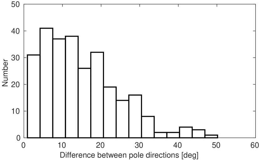
Figure 1: Histogram of differences between the pole directions of models derived from Lowell data and those archived in DAMIT.

3 Results

3.1 Comparison with independent models

From all $\sim 600$ models that successfully passed the tests described in Sect. 2.6, some were already modeled from other photometric data and the models were stored in the Database of Asteroid Models from Inversion Techniques (DAMIT, Ďurech et al., 2010). For this subset, we could compare our results from an inversion of Lowell data with independent models (assumed to be reliable) from DAMIT. In total, there were 279 models in DAMIT for comparison. For these models, we computed the difference between the DAMIT and Lowell rotation periods and also the difference between the pole directions. Out of this set, almost all (275 models) have the same rotation periods (within the uncertainties) and the pole differences $<50^{\circ}$ of arc. The histogram of pole differences between DAMIT and our models is shown in Fig. 1. Although there are some asteroids for which we got differences as large as $\sim 40$–$50^{\circ}$, the mean value is $15^{\circ}$ and the median $13^{\circ}$, which can be interpreted as a typical error in the pole determination that was based on Lowell data, assuming that the poles from DAMIT have smaller errors (typically 5–10^∘).

As an example of the difference between shape models, we show results for asteroid (63) Ausonia. In Fig. 2, we compare our shape model, which we derived from Lowell sparse photometry, with that obtained by inversion of dense lightcurves (Torppa et al., 2003). In general, the shapes derived from sparse photometry are more angular than those derived from dense lightcurves and often have artificial sharp edges.

The four asteroids (5) Astraea, (367) Amicita, (540) Rosamunde, and (4954) Eric, for which we got different solutions to DAMIT, are discussed below. We also discuss the five asteroids – (1753) Mieke, (2425) Shenzen, (6166) Univsima, (11958) Galiani, and (12753) Povenmire – for which there is no model in DAMIT, but the period we derived from the Lowell data does not agree with the data in LCDB.

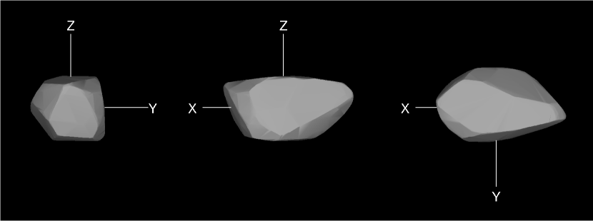
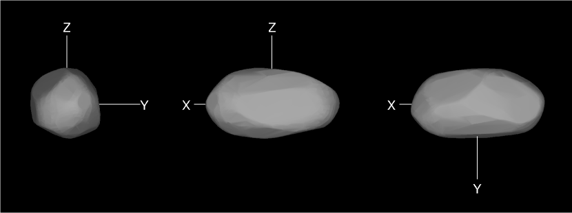
Figure 2: Comparison between the shape model of (63) Ausonia reconstructed from Lowell sparse data (top) and from dense lightcurves (bottom).

(5) Astraea

From Lowell data, we got two pole directions $(\lambda,\beta)=(121^{\circ},-20^{\circ})$ and $(296^{\circ},-15^{\circ})$, the former being about $60^{\circ}$ away from the DAMIT model of Hanuš et al. (2013b) with the pole $(126^{\circ},40^{\circ})$. The DAMIT model agrees with the adaptive optics data as well as with the occultation silhouette from 2008 and it is not clear why there is so large a difference in the pole direction, while the rotation periods are the same and the number of Lowell photometric points is also large (447 points).

(367) Amicita

The model derived from Lowell data has two pole solutions $(17^{\circ},-52^{\circ})$ and $(194^{\circ},-45^{\circ})$ and rotation period of 5.05578 h, while the DAMIT model of Hanuš et al. (2011) has prograde rotation with poles of $(21^{\circ},32^{\circ})$ and $(203^{\circ},38^{\circ}),$ with a significantly different period of 5.05502 h. However, the DAMIT model is based on sparse data from US Naval Observatory and Catalina and only two pieces of lightcurve by Wisniewski et al. (1997) and it might not be correct.

(540) Rosamunde

Although the periodogram obtained with the convex model approach shows a minimum for 9.34780 h – the same as the DAMIT model of Hanuš et al. (2013a) – this minimum was not deep enough to pass the test nr. 1. However, the second-best minimum for a convex model at 7.82166 h appeared as the best solution for the ellipsoid approach and passed all tests leading to a wrong model.

(4954) Eric

The DAMIT model of Hanuš et al. (2013c) has a pole direction of $(86^{\circ},-55^{\circ})$, which is almost exactly opposite to our value of $(261^{\circ},70^{\circ})$. Moreover, even the rotation periods are different by about 0.0003 h, which is more than the uncertainty interval.

(1753) Mieke

The rotation period of 8.9 h was determined by Lagerkvist (1978) from two (1.5 and 5 hours) noisy lightcurves. Given the quality of the data, this period is not in contradiction with our value of 10.19942 h.

(2425) Shenzen

The rotation period of $14.715\pm 0.012$ h was determined by Hawkins & Ditteon (2008). Our value of 9.83818 h is close to 2/3 of their. In the periodogram, there is no significant minimum around 14.7 h.

(6166) Univsima

The lightcurve is published online in the database of R. Behrend. However, the period of 9.6 h is based on only 12 points, which covers about half of the reported period, so we think that this preliminary result is not in contradiction with our period of $\sim 11.4$ h.

(11958) Galiani

This asteroid was observed by Clark (2014), who determined the period $9.8013\pm 0.0023$ h, which does not agree with our value of 8.24720 h. The reason is not clear, because the data of Clark (2014) seem to fit this period correctly. We do not see any significant minimum in $\chi^{2}$ near 9.8 h in the periodogram.

(12753) Povenmire

The period of 12.854 h reported in the LCDB is based on the observations of Gary (2004). However, according to the same author, the correct rotation period that is based on observations from 2010 is $17.5752\pm 0.0008$ h, which agrees with our value.

In summary, the frequency of false positive solutions that pass all reliability tests seems to be sufficiently low, around a few percent. However, the sample of models in DAMIT that we use for comparison is itself biased against low-amplitude long-period asteroids (Marciniak et al., 2015), so the real number of false positive solutions might be higher.

3.2 New models

After applying all the tests described in Sect. 2.6, we selected only those asteroids with no model in DAMIT for publication. These are listed in Tables 4 (models from full interval 2–100 hours) and 4 (models derived from a restricted period interval). The tables list the pole direction(s) (one or two models), the sidereal rotation period (with uncertainty corresponding to the order of the last decimal place). The C/E code means the method by which $P_{\text{min}}$ was found – convex models (C) or ellipsoids (E). In some cases, both methods independently gave the same value of $P_{\text{min}}$ (then CE code). All new shape models and the photometric data are available in DAMIT.

For some of these asteroids, Hanuš et al. (2016) obtained independent models by applying the same lightcurve inversion method on sparse data, which they combined with dense lightcurves. These asteroids (not yet published in DAMIT) are marked by asterisk in the Tables 4 and 4. For all of them (56 in total), our rotation periods agree with those of Hanuš et al. (2016) within their uncertainties and pole directions differ by 10–20 degrees on average. By way of comparison, this is a similar result to the DAMIT models (Sect. 3.1, Fig. 1) and it independently confirms the reliability of our models based on only Lowell data.

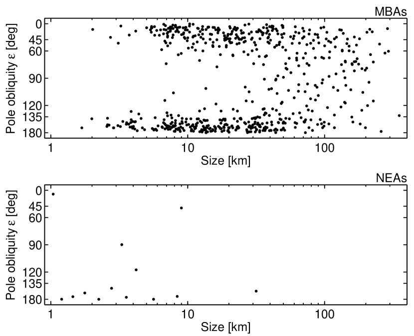
Figure 3: The distribution of pole obliquity $\varepsilon$ as a function of size for 575 main-belt and 13 near-Earth asteroids.

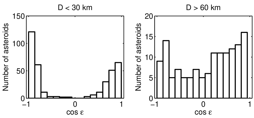
Figure 4: Histograms of the distribution of pole obliquities $\varepsilon$ for asteroids with diameters $<30$ km and $>60$ km, respectively.

3.3 Statistics of pole directions

Together with models from DAMIT, we now have a sample of shape models for 717 asteroids (685 MBAs, 13 NEAs, 10 Mars-crossers, 7 Hungarias, 1 Hilda, and 1 Trojan). The statistical analysis of the pole distribution confirms the previous findings. Namely, the distribution of spin directions is not isotropic (Kryszczyńska et al., 2007). Moreover, the distribution of pole obliquities (an angle between the spin vector and the orbital plane) depends on the size of an asteroid. We plot the dependence of obliquity on the size in Fig. 3 for main-belt (MBAs) and near-Earth (NEAs) asteroids. There is a clear trend of smaller asteroids clustering towards extreme values of obliquity. This was explained by Hanuš et al. (2011) as YORP-induced evolution of spins (Hanuš et al., 2013c). The distribution of obliquities is not symmetric around $90^{\circ}$ (Fig. 4). As noticed by Hanuš et al. (2013c), the retrograde rotators are more concentrated to $-90^{\circ}$, probably because prograde rotators are affected by resonances. For larger asteroids, there is an excess of prograde rotators that might be primordial (Kryszczyńska et al., 2007; Johansen & Lacerda, 2010).

However, the current sample of asteroid models is far from being representative of the whole asteroid population. Because the period search in sparse data is strongly dependent on the lightcurve amplitude – the larger the amplitude the easier is to detect the correct rotation period in noisy data – more elongated asteroids are reconstructed more easily than spherical ones. That is why almost all the asteroids listed in Tables 4 and 4 have large amplidudes of $\gtrsim 0.3$ mag. The lightcurve inversion (based mostly or exclusively on sparse data) is also less efficient for asteroids with poles close to the ecliptic plane because, during some apparitions, we observe them almost pole-on, thus with very small amplitudes. This bias in the method was estimated to be of the order of several tens percent (Hanuš et al., 2011). A much higher discrepancy (factor 3–4) in the successfully recovered pole directions between poles close-to and perpendicular-to the ecliptic was found by Santana-Ros et al. (2015). But even such a large selection effect cannot fully explain the significant “gap” for obliquities between 60–120^∘. To clearly show how the unbiased distribution of pole obliquities looks like, we would have to carry out an extensive simulation on a synthetic population with realistic systematic and random errors to see the bias that is induced by the method, shape, and geometry. This sort of simulation would be more computationally demanding than processing real data from the Lowell database. Therefore, we postpone this investigation for a future paper.

For near-Earth asteroids, the excess of retrograde rotators can be explained by the Yarkovsky-induced delivery mechanism from the main belt through resonances (La Spina et al., 2004), although the number of NEA models in our sample is too small for any reliable statistics.

We also see a clear deviation from a uniform distribution of pole longitudes in Fig. 5. Because of ambiguity in pole direction (often there are two solutions with similar latitudes and the difference in longitudes of about $180^{\circ}$), we plotted the distribution modulo $180^{\circ}$. The histogram shows an excess of longitudes around 50–100^∘. This was already announced by Bowell et al. (2014), who processed the Lowell data set using a different approach, estimated spin-axis longitudes for more than 350,000 asteroids, and revealed an excess of longitudes at 30–110^∘ and a paucity at 120–180^∘. The explanation of this phenomenon remains unclear.

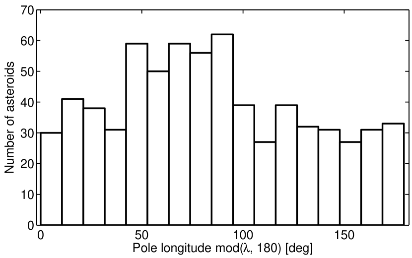
Figure 5: Histograms of the distribution of pole longitude $\lambda$ for 685 main-belt asteroids.

4 Conclusions

The new models presented in this paper significantly enlarge the sample of asteroids for which their spin axis direction and approximate shape are known. Because these models are based on a limited number of data points, the shapes have to be interpreted as only approximations of the real shapes of asteroids. Also the pole directions need to be refined with more data if one is interested in a particular asteroid. However, as an ensemble, the models can be used in future statistical studies of asteroid spins, for example.

We believe that this is only the beginning of a mass production of shape and spin models from sparse photometry. Although the number of models derivable from the Lowell Observatory photometric database is small compared to the total number of asteroids, the potential of Lowell photometry consists in its combination with other data. Even a priori information about the rotation period shrinks the parameter space that has to be scanned, and a local minimum in a large parameters space becomes a global minimum on a restricted interval. Of course, the reliability of this type of model depends critically on the reliability of the period. Lowell photometry can be combined with dense lightcurves that constrain the rotation period. This way, models for about 250 asteroids were derived recently by Hanuš et al. (2016), some of which confirm the models presented in this paper. The database of asteroid rotation periods has been increased dramatically by Waszczak et al. (2015) – their data can also be combined with Lowell photometry, and we expect that other hundreds of models will be reconstructed from this data set. Another promising approach is the combination of sparse photometry with data from the Wide-field Infrared Survey Explorer (WISE) mission (Wright et al., 2010). Although WISE data were observed in mid-infrared wavelengths, Ďurech et al. (2016) showed that thermally emitted flux can be treated as reflected light to derive the correct rotation period and the shape and spin model. This opens up a new possibility, because both Lowell and WISE data are available for tens of thousands of asteroids.

In general, the combination of more data sources is always better than using them separately. By using Lowell photometry with dense lightcurves, WISE data, photometry from Gaia, etc., the number of available models will increase and the statistical studies of spin and shape distribution will become more robust, being based on larger sets of models. Nevertheless, any inference based on the models derived from lightcurves (and sparse lightcurves in particular) has to take into account that the sample of models is biased against more spherical shapes with low lightcurve amplitudes and poles near the plane of ecliptic.

longtabler l r r r r @ d @ d l l l r c List of new asteroid models derived from the full period interval 2–100 hours. For each asteroid, there is one or two pole directions in the ecliptic coordinates $(\lambda,\beta)$, the sidereal rotation period $P$, rotation period from LCDB $P_{\mathrm{LCDB}}$ and its quality code $U$ (if available), the minimum and maximum lightcurve amplitude $A_{\text{min}}$, $A_{\text{max}}$, respectively, the number of data points $N$, and the method which was used to derive the unique rotation period: C – convex inversion, E – ellipsoids, CE – both methods gave the same unique period. The accuracy of the sidereal rotation period is of the order of the last decimal place given. Asteroids marked with $\ast$ were independently confirmed by Hanuš et al. (2016).
Asteroid $\lambda_{1}$ $\beta_{1}$ $\lambda_{2}$ $\beta_{2}$ $P$ $P_{\mathrm{LCDB}}$ $A_{\text{min}}$ $A_{\text{max}}$ $U$ $N$ method
number name/designation [deg] [deg] [deg] [deg] [h] [h] [mag] [mag]
continued.
Asteroid $\lambda_{1}$ $\beta_{1}$ $\lambda_{2}$ $\beta_{2}$ $P$ $P_{\mathrm{LCDB}}$ $A_{\text{min}}$ $A_{\text{max}}$ $U$ $N$ method
number name/designation [deg] [deg] [deg] [deg] [h] [h] [mag] [mag]
136 Austria^∗ 118 57 333 75 11.49665 11.4969 0.37 3 401 CE
163 Erigone 276 $-69$ 16.1402 16.136 0.32 0.37 3 483 E
186 Celuta 88 $-54$ 235 $-77$ 19.8435 19.842 0.4 0.55 3 406 C
254 Augusta^∗ 56 $-69$ 218 $-75$ 5.89503 5.8961 0.56 0.75 3$-$ 371 CE
263 Dresda^∗ 101 55 280 58 16.8138 16.809 0.32 0.55 3 605 E
274 Philagoria^∗ 138 $-52$ 303 $-58$ 17.94072 17.96 0.43 0.51 3 460 E
296 Phaetusa^∗ 145 53 326 60 4.538091 4.5385 0.38 0.50 3 340 C
381 Myrrha^∗ 3 48 160 77 6.57198 6.572 0.35 0.36 3 496 E
407 Arachne^∗ 64 $-49$ 268 $-63$ 22.6264 22.62 0.31 0.45 2 433 C
427 Galene 72 $-57$ 272 $-75$ 3.706036 3.705 0.55 0.68 3 394 CE
474 Prudentia^∗ 150 $-58$ 297 $-46$ 8.57228 8.572 0.53 0.90 3 374 E
482 Petrina^∗ 94 2 274 37 11.79212 11.7922 0.07 0.56 3 337 E
518 Halawe 120 $-66$ 292 $-58$ 14.31765 14.310 0.50 0.55 3 439 E
520 Franziska^∗ 122 $-50$ 301 $-59$ 16.5044 16.507 0.35 0.51 3 384 CE
523 Ada 152 $-70$ 357 $-70$ 10.03242 10.03 0.52 0.70 3 343 CE
616 Elly 60 62 250 44 5.29770 5.297 0.34 0.44 3 368 CE
620 Drakonia 138 56 316 47 5.48711 5.487 0.52 0.65 3 345 E
632 Pyrrha^∗ 72 $-64$ 249 $-72$ 4.116854 4.1167 0.40 3 487 CE
650 Amalasuntha 46 51 16.57586 16.582 0.45 0.49 3 435 E
686 Gersuind^∗ 127 56 6.31240 6.3127 0.30 0.37 3 400 E
689 Zita 8 $-72$ 256 $-61$ 6.42391 6.425 0.30 0.62 3 369 E
698 Ernestina^∗ 193 $-68$ 5.03661 5.0363 0.30 0.69 3 459 C
718 Erida 78 $-56$ 257 $-52$ 17.4462 17.447 0.31 0.37 3 430 E
749 Malzovia^∗ 53 37 242 46 5.92749 5.9279 0.30 3$-$ 423 E
784 Pickeringia^∗ 99 67 283 30 13.16995 13.17 0.20 0.40 2 437 E
789 Lena 192 39 5.84239 5.848 0.40 0.50 3 328 E
829 Academia 71 $-41$ 245 $-67$ 7.89321 7.891 0.36 0.44 3$-$ 436 E
877 Walkure^∗ 68 58 253 61 17.4217 17.424 0.33 0.44 3$-$ 596 E
881 Athene^∗ 123 $-58$ 337 $-47$ 13.89449 13.895 0.39 0.53 3$-$ 376 CE
955 Alstede 54 38 240 13 5.18735 5.19 0.26 0.27 3 401 E
996 Hilaritas 100 $-56$ 281 $-57$ 10.05154 10.05 0.63 0.70 3 442 CE
998 Bodea 7 $-59$ 8.57412 8.574 0.68 3 262 E
1017 Jacqueline 7 55 170 65 7.87149 7.87 0.6 0.72 3 491 CE
1035 Amata 31 69 247 29 9.08215 9.081 0.41 0.44 3 305 E
1050 Meta 60 $-42$ 198 $-79$ 6.14188 6.142 0.46 3 325 E
1061 Paeonia 155 $-50$ 7.99710 6. 0.5 2$-$ 314 E
1075 Helina 123 $-33$ 284 $-34$ 44.6768 44.9 0.64 3$-$ 421 C
1081 Reseda 92 $-69$ 256 $-76$ 7.30136 7.3002 0.34 3 410 E
1082 Pirola 123 $-42$ 300 $-38$ 15.8540 15.8525 0.53 0.60 3 528 E
1098 Hakone 40 43 7.14117 7.142 0.35 0.40 3 382 E
1119 Euboea^∗ 71 61 280 54 11.39823 11.41 0.46 0.50 3 461 E
1121 Natascha 16 59 209 50 13.19717 13.197 0.51 3 415 E
1127 Mimi 224 $-57$ 12.74557 12.749 0.72 0.95 3 357 CE
1135 Colchis^∗ 7 $-54$ 168 $-56$ 23.4827 23.47 0.45 2 409 C
1147 Stavropolis 78 $-50$ 267 $-51$ 5.66079 5.66 0.42 3 372 E
1187 Afra 40 34 226 13 14.06993 14.0701 0.38 0.40 3 374 E
1204 Renzia^∗ 130 $-44$ 312 $-51$ 7.88697 7.885 0.42 3 528 E
1206 Numerowia 64 $-50$ 271 $-69$ 4.77529 4.7743 0.63 3 322 CE
1219 Britta 72 $-66$ 241 $-66$ 5.57556 5.575 0.48 0.75 3 387 E
1230 Riceia 37 $-63$ 6.67317 293 CE
1231 Auricula 57 $-57$ 225 $-85$ 3.981580 3.9816 0.75 3 292 E
1245 Calvinia 52 $-51$ 235 $-43$ 4.85148 4.84 0.37 0.7 3 410 E
1248 Jugurtha 254 $-89$ 12.19047 12.910 0.70 1.4 3 381 C
1251 Hedera 124 $-70$ 266 $-62$ 19.9020 19.9000 0.41 0.61 3$-$ 415 E
1275 Cimbria 85 $-61$ 271 $-31$ 5.65454 5.65 0.40 0.57 3 352 E
1281 Jeanne 153 19 338 32 15.30379 15.2 0.45 2 470 E
1299 Mertona 73 35 253 56 4.97691 4.977 0.46 0.59 3 369 E
1312 Vassar^∗ 104 $-50$ 250 $-29$ 7.93189 7.932 0.35 3 317 E
1320 Impala 151 $-57$ 254 $-70$ 6.17081 6.167 0.40 0.52 2+ 353 E
1334 Lundmarka 79 $-75$ 6.25033 6.250 0.70 3$-$ 496 CE
1339 Desagneauxa 63 53 225 42 9.37514 9.380 0.45 0.48 3 465 E
1349 Bechuana 153 32 314 46 15.6873 15.692 0.30 3$-$ 412 E
1350 Rosselia 67 $-64$ 246 $-58$ 8.14008 8.140 0.3 0.54 3 425 E
1391 Carelia 21 $-79$ 208 $-43$ 5.87822 295 E
1400 Tirela 58 $-80$ 297 $-41$ 13.35384 13.356 0.55 2 281 E
1459 Magnya^∗ 73 $-54$ 198 $-55$ 4.679102 4.678 0.57 0.85 3 363 E
1484 Postrema 19 44 250 64 12.18978 12.1923 0.22 0.23 3$-$ 312 E
1493 Sigrid 183 69 350 69 43.1795 43.296 0.38 0.6 2 452 C
1494 Savo 50 $-65$ 233 $-68$ 5.35059 5.35011 0.45 0.52 3 486 C
1500 Jyvaskyla 123 $-75$ 268 $-79$ 8.82750 248 C
1545 Thernoe 164 $-75$ 352 $-80$ 17.20321 17.20 0.76 3 281 E
1547 Nele 159 28 318 50 7.09742 7.100 0.18 0.45 3$-$ 343 E
1548 Palomaa 72 $-61$ 232 $-32$ 7.49966 7.4961 0.50 3 353 E
1551 Argelander 3 $-81$ 183 $-72$ 4.058350 453 CE
1557 Roehla 124 $-38$ 329 $-57$ 5.67899 334 CE
1561 Fricke 320 71 15.15330 395 E
1597 Laugier 345 $-78$ 8.02272 321 E
1619 Ueta 99 49 295 37 2.718238 2.720 0.32 0.44 3 350 E
1623 Vivian 52 $-66$ 229 $-56$ 20.5235 20.5209 0.85 3$-$ 316 C
1643 Brown 140 64 353 84 5.93124 5.932 0.48 3 497 CE
1648 Shajna^∗ 94 47 278 50 6.41368 6.4140 0.65 3 391 E
1672 Gezelle^∗ 44 73 234 82 40.6821 40.72 0.2 0.56 3 366 C
1676 Kariba^∗ 71 74 279 56 3.167336 3.1673 0.51 0.65 3 342 CE
1687 Glarona 132 76 274 70 6.49595 6.3 0.75 3 375 CE
1730 Marceline^∗ 95 56 303 81 3.836550 3.837 0.94 1.00 3 268 E
1733 Silke 141 $-63$ 302 $-58$ 7.89457 277 E
1738 Oosterhoff 121 $-62$ 301 $-80$ 4.448955 4.4486 0.48 0.54 3 371 C
1743 Schmidt 69 $-62$ 261 $-53$ 17.4599 17.45 0.36 3 381 E
1753 Mieke 121 67 321 35 10.19942 8.8 0.2 2 413 E
1758 Naantali 150 $-60$ 5.47369 5.4699 0.44 3 446 E
1768 Appenzella 39 45 227 40 5.18335 5.1839 0.53 3 395 CE
1774 Kulikov 54 $-50$ 237 $-46$ 3.830791 518 E
1792 Reni 122 $-41$ 260 $-50$ 15.94121 15.95 0.54 3$-$ 319 E
1793 Zoya^∗ 52 59 227 59 5.75187 5.753 0.40 2+ 398 CE
1801 Titicaca 48 51 260 57 3.211233 3.2106 0.50 3 379 CE
1814 Bach 126 66 317 64 7.23954 221 CE
1819 Laputa 149 $-48$ 9.79965 9.8004 0.51 3 394 CE
1825 Klare^∗ 115 $-61$ 315 $-69$ 4.742885 4.744 0.70 0.90 3 336 CE
1838 Ursa^∗ 51 66 286 32 16.16358 16.141 0.80 3 346 C
1840 Hus 298 $-77$ 4.749057 4.780 0.85 2$-$ 549 E
1841 Masaryk 122 62 305 59 7.54301 7.53 0.52 2+ 406 E
1855 Korolev 90 52 262 64 4.656199 4.6568 0.75 0.76 3 370 C
1900 Katyusha 94 $-46$ 291 $-48$ 9.50358 9.4999 0.56 0.74 3 283 E
1942 Jablunka 156 $-73$ 8.91158 225 E
1945 Wesselink 190 $-78$ 336 $-60$ 3.547454 445 E
1949 Messina 138 $-64$ 326 $-51$ 3.649308 3.6491 0.37 3 323 CE
1978 Patrice 21 13 203 18 5.881213 365 CE
1985 Hopmann 107 $-81$ 17.4787 17.480 0.36 0.44 3 272 E
1997 Leverrier 96 46 274 40 8.01532 301 E
2313 Aruna^∗ 94 $-80$ 283 $-70$ 8.88618 8.90 0.79 3 715 E
2381 Landi^∗ 54 $-87$ 237 $-45$ 3.986045 3.989 0.75 1.04 3 364 E
2395 Aho 160 47 340 46 7.88033 751 E
2425 Shenzhen 50 58 265 40 9.83818 14.715 0.80 3 551 E
2483 Guinevere 19 70 194 59 14.73081 14.733 1.34 1.38 3 317 E
2528 Mohler 56 $-64$ 246 $-54$ 6.49130 641 E
2581 Radegast 57 56 230 53 8.75121 573 CE
2630 Hermod 74 50 256 45 19.4283 578 E
2659 Millis^∗ 117 $-55$ 294 $-52$ 6.12464 6.132 0.53 0.84 3 566 C
2836 Sobolev 82 $-51$ 270 $-79$ 4.754883 560 E
3086 Kalbaugh 63 $-51$ 5.17907 5.180 0.47 0.76 3 383 C
3261 Tvardovskij 90 65 280 68 5.36852 665 E
3281 Maupertuis 62 $-66$ 231 $-74$ 6.72984 6.7295 1.22 3 453 E
3286 Anatoliya 52 51 293 76 5.81029 410 CE
3375 Amy 168 $-50$ 343 $-49$ 3.255633 486 E
3407 Jimmysimms 34 53 259 82 6.82069 6.819 0.93 0.95 3 457 E
3544 Borodino^∗ 104 $-57$ 267 $-53$ 5.43459 5.442 0.60 0.65 3 515 E
3573 Holmberg 142 50 318 52 6.54245 6.5431 0.91 1.03 3 577 C
3735 Trebon 51 $-54$ 236 $-69$ 8.47251 568 E
3746 Heyuan 170 66 333 70 16.3010 538 E
3758 Karttunen 74 $-72$ 202 $-52$ 12.50101 396 CE
3786 Yamada^∗ 100 54 205 60 4.032946 4.034 0.40 0.65 3 463 E
3822 Segovia 43 58 265 72 11.03204 585 E
3910 Liszt 104 $-46$ 290 $-66$ 4.736280 4.73 0.60 3 423 E
4037 Ikeya 92 67 270 44 4.057537 485 E
4877 Humboldt 218 $-77$ 340 $-55$ 3.491213 450 E
5006 Teller 84 66 301 57 10.90225 10.898 0.69 3 474 E
5195 Kaendler 67 $-59$ 212 $-50$ 5.33756 537 E
5299 Bittesini 76 60 251 49 4.679660 599 CE
5488 Kiyosato 19 23 242 62 8.76307 449 E
5489 Oberkochen^∗ 23 $-62$ 194 $-38$ 5.62439 5.625 0.40 0.51 3 470 E
5494 1933 UM1 137 $-65$ 323 $-62$ 5.72752 612 CE
5685 Sanenobufukui 122 $-63$ 327 $-58$ 3.387871 518 CE
5723 Hudson 72 $-73$ 255 $-58$ 4.475115 472 E
5776 1989 UT2^∗ 105 $-76$ 350 $-46$ 4.340787 473 E
5929 1974 XT 130 $-71$ 244 $-40$ 3.759432 3.7596 1.01 3 358 E
5993 Tammydickinson 52 $-65$ 241 $-78$ 9.44711 546 E
6136 Gryphon 134 57 337 63 16.4683 16.476 0.61 3 602 E
6161 Vojno-Yasenetsky 64 70 217 41 7.98095 393 E
6166 Univsima 80 $-42$ 242 $-59$ 11.37655 9.6 0.6 2 425 E
6276 Kurohone 147 63 322 62 6.34850 441 E
6410 Fujiwara^∗ 148 $-59$ 296 $-81$ 7.00667 7.0073 0.80 0.85 3 552 E
6422 Akagi 213 $-38$ 7.74756 430 E
6590 Barolo 171 59 313 63 8.35928 460 CE
6671 1994 NC1 69 57 204 78 5.22042 463 E
6719 Gallaj 60 $-63$ 252 $-59$ 4.429487 515 E
6882 Sormano 43 $-33$ 248 $-58$ 3.998344 396 E
7001 Noether 13 $-66$ 9.58191 421 E
7072 Beijingdaxue 72 56 262 64 5.304419 549 E
7106 Kondakov 63 58 268 81 7.59690 515 E
7289 Kamegamori 108 $-39$ 268 $-54$ 3.831182 538 C
7318 Dyukov 65 $-64$ 239 $-44$ 4.856335 497 E
7835 1993 MC 72 $-64$ 288 $-55$ 7.43019 473 E
7896 Svejk 86 36 266 35 16.20582 500 E
7964 1995 DD2 74 $-73$ 264 $-49$ 10.22553 532 E
8573 Ivanka 100 $-70$ 344 $-78$ 8.03312 454 E
9440 1997 FZ1 97 $-64$ 278 $-65$ 5.196349 485 E
9971 Ishihara 42 76 223 60 6.71574 559 E
10281 1981 EE45 183 $-88$ 7.57192 462 E
10472 1981 EO20 73 37 249 43 5.98599 344 C
10627 Ookuninushi 3 49 204 89 4.334986 394 E
11052 1990 WM 194 $-49$ 351 $-78$ 5.06904 471 E
11148 Einhardress 121 $-69$ 296 $-64$ 7.77240 378 E
11700 1998 FT115 82 $-64$ 280 $-72$ 5.52303 596 E
11958 Galiani 12 47 8.24720 9.801 0.96 2+ 541 E
11995 1995 YB1 70 $-80$ 238 $-68$ 12.66498 398 E
12384 Luigimartella 4 $-50$ 160 $-60$ 6.44220 517 E
12551 1998 QQ39 123 50 299 44 11.19841 571 E
12753 Povenmire 138 $-28$ 295 $-48$ 17.5740 12.854 0.45 2 424 E
12774 Pfund 121 53 308 62 7.34295 174 E
12979 1978 SB8 45 $-68$ 203 $-62$ 5.78331 349 C
13059 Ducuroir 117 71 311 73 13.84864 560 E
13338 1998 SK119 86 $-42$ 240 $-70$ 4.129105 474 E
13535 1991 RS13 127 $-64$ 318 $-60$ 5.22705 390 E
13952 1990 SN6 13 58 193 67 7.35225 526 E
14031 1994 WF2 41 $-62$ 180 $-60$ 2.900652 509 E
14044 1995 VS1 95 $-47$ 253 $-57$ 9.25874 499 E
14203 Hocking 106 81 240 52 9.08566 393 E
14691 2000 AK119 38 $-54$ 248 $-68$ 3.652412 3.652 0.70 0.78 3 441 E
15677 1980 TZ5 75 $-64$ 226 $-75$ 5.61479 491 E
16216 2000 DR4 130 $-66$ 10.36816 480 E
16786 1997 AT1 178 56 307 60 4.020902 296 E
16955 1998 KU48 122 $-48$ 264 $-51$ 5.26062 387 E
17111 1999 JH52 157 46 328 62 8.89847 629 E
19608 1999 NC57 69 $-68$ 306 $-68$ 9.18995 513 E
20329 Manfro 92 $-55$ 258 $-63$ 8.80724 395 E
20570 Molchan 40 $-52$ 244 $-59$ 4.132007 485 E
20725 1999 XP120 170 67 334 45 3.601296 488 E
21411 Abifraeman 249 $-63$ 11.02020 409 E
22018 1999 XK105 61 45 228 31 17.0575 373 C
22298 1990 EJ 64 $-42$ 244 $-72$ 2.985538 530 C
23578 Baedeker 141 $-53$ 8.17154 382 C
23707 1997 TZ7 185 79 334 35 5.06632 381 E
23873 1998 RL76 56 $-74$ 13.86111 323 E
26241 1998 QY40 40 45 12.83303 380 C
26387 1999 TG2 94 $-46$ 325 $-79$ 5.14720 460 E
26460 2000 AZ120 9 $-87$ 230 $-47$ 5.45444 5.48 0.90 2 326 E
27225 1999 GB17 72 54 266 31 3.853858 480 C
28133 1998 SS130 126 $-49$ 310 $-56$ 5.46284 408 CE
29308 1993 UF1 71 $-56$ 246 $-83$ 9.79348 9.810 0.83 0.94 3 365 E
29777 1999 CK46 32 56 224 40 3.627265 460 E
31060 1996 TB6^∗ 103 $-52$ 253 $-76$ 5.104323 5.103 0.80 3 394 E
32575 2001 QY78 60 $-70$ 223 $-64$ 4.535495 4.5344 0.86 3 324 E
32799 1990 QN1 71 75 258 72 9.49636 337 E
33776 1999 RB158 46 64 247 42 16.9593 426 E
33854 2000 HH53 114 $-56$ 236 $-78$ 4.423484 348 E
33974 2000 ND17 132 $-55$ 347 $-65$ 4.67868 340 E
34318 2000 QV192 81 $-70$ 237 $-36$ 6.35105 198 E
35218 1994 WU2 138 $-56$ 304 $-68$ 11.56991 353 E
35928 1999 JV107 137 $-52$ 302 $-75$ 7.26361 279 E
35965 1999 LH13 63 $-70$ 245 $-55$ 6.76072 387 E
36303 2000 JM54 55 $-48$ 225 $-46$ 4.93652 368 E
36487 2000 QJ42 127 $-66$ 332 $-50$ 8.14982 333 E
36944 2000 SD249 96 $-69$ 295 $-76$ 6.09677 188 C
40104 1998 QE4 144 $-87$ 4.475241 443 E
40478 1999 RT54 184 $-66$ 358 $-65$ 3.886734 286 C
40806 1999 TX41 82 $-69$ 269 $-64$ 6.41500 198 C
43163 1999 XB127 154 $-59$ 5.20660 298 C
43574 2001 FU192 104 $-36$ 279 $-49$ 4.324751 239 E
45864 2000 UO97 44 $-66$ 179 $-84$ 5.13544 436 E
46376 2001 XD3 121 55 5.73569 278 E
47508 2000 AQ58 12 $-49$ 196 $-26$ 5.05521 349 E
48268 2002 AK1 72 $-69$ 234 $-35$ 4.250546 406 E
48842 1998 BA44 86 83 254 43 6.17996 383 E
52723 1998 GP2 86 $-39$ 224 $-56$ 11.90781 329 E
54850 2001 OZ11 20 $-68$ 189 $-48$ 4.222157 283 E
55200 2001 RO19 14 $-70$ 186 $-58$ 18.3910 233 E
64480 2001 VG45 128 $-60$ 265 $-72$ 6.49717 233 E
66076 1998 RD53 100 $-54$ 233 $-66$ 8.93855 485 E
69117 2003 EX2 13 70 4.74608 215 E
71011 1999 XE45 91 $-24$ 264 $-31$ 4.69449 115 C
74155 1998 QK93 264 50 15.9680 393 E
75167 1999 VF128 190 $-56$ 350 $-55$ 10.27743 280 C
75495 1999 XM181 64 $-32$ 252 $-64$ 14.69041 200 E
76214 2000 EV64 168 28 9.27775 132 C
77677 2001 MA25 139 $-69$ 326 $-55$ 5.304712 253 E
78420 2002 QU40 123 $-46$ 327 $-45$ 4.91365 4.90 1.1 2 193 E
79436 1997 TD6 70 $-53$ 201 $-68$ 3.635352 207 E
80112 1999 RN61 70 $-58$ 247 $-39$ 4.923622 157 E
81740 2000 JA46 100 $-72$ 310 $-47$ 9.34151 272 E
81911 2000 NV9 136 23 334 49 6.95480 288 E
82642 2001 PX5 53 37 241 67 11.61144 178 E
85489 1997 SV2 317 $-56$ 5.79502 81 E
85532 1997 WD21 117 $-75$ 4.76820 230 E
89764 2002 AW61 8 $-45$ 152 $-60$ 5.93513 278 E
91063 1998 FX62 53 $-44$ 191 $-60$ 11.66510 255 C
94808 2001 XM167 9 $-59$ 197 $-63$ 10.66092 104 E
96461 1998 HS36 166 $-60$ 344 $-72$ 12.67641 115 E
97346 2000 AF10 11 42 222 50 7.65364 394 E
99667 2002 JO1 86 $-57$ 262 $-42$ 5.07877 199 C

longtabler l r r r r @ d @ d l l l r c List of new asteroid models derived from a restricted period interval centered at $P_{\mathrm{LCDB}}$. The meaning of columns is the same as in Table 4. Asteroids marked with $\ast$ were independently confirmed by Hanuš et al. (2016).
Asteroid $\lambda_{1}$ $\beta_{1}$ $\lambda_{2}$ $\beta_{2}$ $P$ $P_{\mathrm{LCDB}}$ $A_{\text{min}}$ $A_{\text{max}}$ $U$ $N$ method
number name/designation [deg] [deg] [deg] [deg] [h] [h] [mag] [mag]
continued.
Asteroid $\lambda_{1}$ $\beta_{1}$ $\lambda_{2}$ $\beta_{2}$ $P$ $P_{\mathrm{LCDB}}$ $A_{\text{min}}$ $A_{\text{max}}$ $U$ $N$ method
number name/designation [deg] [deg] [deg] [deg] [h] [h] [mag] [mag]
60 Echo 91 $-25$ 272 $-17$ 25.2285 25.208 0.07 0.22 3 446 E
116 Sirona 51 $-53$ 222 $-53$ 12.03251 12.028 0.42 0.55 3 454 C
138 Tolosa 49 $-42$ 222 $-39$ 10.10306 10.101 0.18 0.45 3 528 E
176 Iduna 83 24 219 68 11.28784 11.2877 0.14 0.43 3 491 E
214 Aschera 123 $-37$ 306 $-42$ 6.83369 6.835 0.20 0.22 3 386 E
239 Adrastea 226 $-70$ 18.4717 18.4707 0.34 0.51 3 416 E
270 Anahita^∗ 30 $-35$ 205 $-48$ 15.05950 15.06 0.25 0.34 3 492 C
353 Ruperto-Carola^∗ 47 $-55$ 220 $-46$ 2.738962 2.73898 0.32 3 368 E
391 Ingeborg^∗ 305 $-52$ 26.4149 26.391 0.22 0.79 3 409 E
394 Arduina^∗ 0 $-79$ 191 $-49$ 16.62157 16.5 0.28 0.54 3 395 CE
513 Centesima 149 4 332 15 5.32399 5.23 0.18 0.45 3 460 C
636 Erika 13 $-70$ 176 $-60$ 14.60771 14.603 0.29 0.33 3 498 E
670 Ottegebe^∗ 127 77 304 68 10.03991 10.045 0.34 0.35 3 540 C
682 Hagar^∗ 93 $-71$ 277 $-35$ 4.850417 4.8503 0.49 0.52 3 334 C
700 Auravictrix 54 33 249 47 6.07489 6.075 0.18 0.43 3 404 CE
706 Hirundo^∗ 91 70 250 45 22.0161 22.027 0.39 0.9 3 365 E
744 Aguntina 44 $-58$ 227 $-51$ 17.4690 17.47 0.50 3 388 CE
762 Pulcova^∗ 20 $-12$ 196 $-42$ 5.83977 5.839 0.18 0.30 3 408 E
769 Tatjana 176 54 347 38 35.0637 35.08 0.30 0.33 3$-$ 437 E
844 Leontina 302 68 6.78303 6.7859 0.20 0.26 3 415 E
885 Ulrike 13 $-64$ 207 $-60$ 4.906164 4.90 0.55 0.72 3 416 C
918 Itha 59 $-59$ 249 $-72$ 3.473810 3.47393 0.15 0.30 3 350 E
943 Begonia 209 $-75$ 15.6593 15.66 0.24 0.34 3 363 E
968 Petunia 355 $-78$ 61.160 61.280 0.38 3 361 CE
979 Ilsewa 352 $-66$ 42.8982 42.61 0.30 0.31 3 370 E
1077 Campanula 178 76 313 59 3.850486 3.85085 0.24 0.40 3 361 E
1083 Salvia 165 $-59$ 358 $-58$ 4.281429 4.23 0.61 3 277 C
1150 Achaia^∗ 126 $-65$ 315 $-60$ 61.071 60.99 0.72 3 396 CE
1294 Antwerpia 128 $-66$ 246 $-76$ 6.62521 6.63 0.35 0.42 3 317 E
1332 Marconia 37 31 220 31 19.2264 19.16 0.30 3 408 E
1352 Wawel^∗ 37 55 201 52 16.9542 16.97 0.35 0.44 3 356 C
1379 Lomonosowa 72 $-84$ 265 $-46$ 24.4846 24.488 0.63 3 359 E
1407 Lindelof 147 36 31.0941 31.151 0.34 3 397 CE
1449 Virtanen^∗ 89 61 302 61 30.5006 30.495 0.08 0.69 3$-$ 354 E
1486 Marilyn^∗ 83 $-57$ 270 $-62$ 4.566945 4.566 0.40 0.48 3 492 C
1496 Turku 75 $-75$ 6.47375 6.47 0.51 3$-$ 486 CE
1521 Seinajoki 63 $-18$ 230 $-37$ 4.328159 4.32 0.15 3 331 C
1592 Mathieu 94 $-14$ 269 $-7$ 28.4821 28.46 0.50 2+ 302 E
1716 Peter 52 $-60$ 252 $-52$ 11.51720 11.514 0.52 3 348 CE
1723 Klemola 52 $-54$ 239 $-56$ 6.25609 6.2545 0.16 0.33 3 484 E
1820 Lohmann^∗ 62 67 250 58 14.04497 14.0554 0.40 0.55 3 281 E
1833 Shmakova 88 47 336 84 3.838235 3.93 0.38 3 355 E
1858 Lobachevskij 80 50 255 48 5.41208 5.413 0.30 0.48 2+ 390 E
1860 Barbarossa 45 30 238 63 3.254853 3.255 0.28 0.35 3 404 E
1906 Naef 72 $-70$ 11.00818 11.009 0.92 0.96 3 319 C
2064 Thomsen 118 $-72$ 334 $-56$ 4.244023 4.233 0.62 3 550 E
2275 Cuitlahuac 9 $-65$ 6.29005 6.2891 1.10 3 536 E
3015 Candy 142 $-26$ 346 $-70$ 4.625223 4.625 0.50 1.05 3 450 E
3773 Smithsonian^∗ 121 $-62$ 6.98132 6.9804 1.04 3 622 C
4089 Galbraith 64 69 218 50 4.91316 4.9123 0.68 3 687 C
4265 Kani^∗ 74 67 277 72 5.727574 5.7279 0.75 3 730 CE
4641 1990 QT3 178 $-46$ 359 $-50$ 5.313079 5.3126 0.88 3 541 C
4801 Ohre 121 $-74$ 266 $-85$ 31.9990 32.000 0.50 0.60 3 581 CE
4896 Tomoegozen 276 $-66$ 8.87996 8.869 0.65 3 371 CE
4995 1984 QR 243 68 355 70 26.3920 26.37 0.82 3$-$ 261 E
5738 Billpickering 2 $-66$ 10.38264 10.4 0.45 3 118 E
6406 1992 MJ^∗ 17 $-61$ 216 $-52$ 6.81816 6.819 1.10 1.18 3 508 CE
6487 Tonyspear 165 $-90$ 74.501 74.91 1.24 3$-$ 372 C
6510 Tarry 84 $-72$ 249 $-37$ 6.36490 6.370 0.50 0.54 3 376 E
7783 1994 JD 70 $-71$ 31.8661 31.83 0.85 3 265 E
9983 Rickfienberg 120 $-58$ 248 $-77$ 5.29616 5.2963 1.30 3 371 C
12045 Klein 77 $-22$ 9.00648 8.9686 0.55 3$-$ 453 E
14257 2000 AR97 57 67 13.57929 13.584 0.67 3 514 C
28887 2000 KQ58^∗ 11 $-61$ 191 $-21$ 6.84315 6.8429 0.55 3 368 E
31485 1999 CM51 94 $-36$ 316 $-56$ 6.00262 6.001 0.65 0.68 3 375 E
34484 2000 SR124^∗ 236 $-55$ 6.17519 6.174 0.80 2+ 473 C
44600 1999 RU10 267 $-24$ 6.21130 6.211 0.98 1.09 3 310 C
80276 1999 XL32 60 38 275 63 5.57148 5.56 0.77 3$-$ 258 C
88161 2000 XK18 195 53 340 70 6.80480 6.806 0.80 3 429 C