Cycle bases of reduced powers of graphs

Abstract

We define what appears to be a new construction. Given a graph $G$ and a positive integer $k$, the reduced $k$th power of $G$, denoted $G^{(k)}$, is the configuration space in which $k$ indistinguishable tokens are placed on the vertices of $G$, so that any vertex can hold up to $k$ tokens. Two configurations are adjacent if one can be transformed to the other by moving a single token along an edge to an adjacent vertex. We present propositions related to the structural properties of reduced graph powers and, most significantly, provide a construction of minimum cycle bases of $G^{(k)}$.

The minimum cycle basis construction is an interesting combinatorial problem that is also useful in applications involving configuration spaces. For example, if $G$ is the state-transition graph of a Markov chain model of a stochastic automaton, the reduced power $G^{(k)}$ is the state-transition graph for $k$ identical (but not necessarily independent) automata. We show how the minimum cycle basis construction of $G^{(k)}$ may be used to confirm that state-dependent coupling of automata does not violate the principle of microscopic reversibility, as required in physical and chemical applications.

Keywords: graph products; Markov chains; cycle spaces.

Math. Subj. Class.: 05C76, 60J27

1 Introduction

Time-homogenous Markov chains [1] are used as a mathematical formalism in applications as diverse as computer systems performance analysis [2], queuing theory in operations research [3], simulation and analysis of stochastic chemical kinetics [4], and biophysical modeling of ion channel gating [5].

Many properties of a Markov chain, such its rate of mixing and its steady-state probability distribution, can be numerically calculated using its transition matrix [6]. A continuous-time Markov chain $X(t)$ ($t\geq 0$) with a finite number of states $\{1,\ldots,\eta\}$ is defined by an initial probability distribution, $\pi_{i}(0)=\Pr\{X(0)=i\}$, and a transition matrix $Q=(q_{ij})$ where $1\leq i,j\leq\eta$, $q_{ij}\geq 0$ for $i\neq j$ and $q_{ii}=-\sum_{j\neq i}q_{ij}$, so called because, for $i\neq j$, $q_{ij}=\lim_{dt\rightarrow 0}\Pr\{X(t+dt)=j|X(t)=i\}/dt$. The requirement that $Q$ has zero row sums, $\sum_{j}q_{ij}=0$, corresponds to conservation of probability, $\sum_{i}\pi_{i}(t)=1$, in the ordinary differential equation initial value problem, $d\boldsymbol{\pi}/dt=\boldsymbol{\pi}Q$ with initial condition $\boldsymbol{\pi}(0)$, solved by the time-dependent discrete probability distribution $\boldsymbol{\pi}(t)=(\pi_{1}(t),\ldots,\pi_{\eta}(t))$ where $\pi_{i}(t)=\Pr\{X(t)=i\}$.

A CTMC with a single communicating class of $\eta<\infty$ states is irreducible, positive recurrent, and has a unique steady-state probability distribution that solves $\bar{\boldsymbol{\pi}}Q=\boldsymbol{0}$ subject to $\sum_{i}\bar{\pi}_{i}=1$ (by the Perron-Frobenius theorem). The Perron vector and steady-state distribution $\bar{\boldsymbol{\pi}}$ is the limiting probability distribution of the Markov chain, $\lim_{t\rightarrow\infty}\|\boldsymbol{\pi}(t)-\bar{\boldsymbol{\pi}}\|=0$, for any initial condition satisfying conservation of probability, $\sum_{i}\pi_{i}(0)=1$. In general, the calculation of steady-state distributions and other properties for Markov chains with $\eta$ states requires algorithms of $\mathcal{O}(\eta^{3})$ complexity.

Many open questions in the physical and biological sciences involve the analysis of systems that are naturally modeled as a collection of interacting stochastic automata [7, 8, 9]. Unfortunately, representing a stochastic automata network as a single master Markov chain suffers from the computational limitation that the aggregate number of states is exponential in the number of components. For example, the transition matrix for $k$ coupled stochastic automata, each of which can be represented by an $v$-state Markov chain, has $\eta=v^{k}$ states and requires algorithms of $\mathcal{O}(v^{3k})$ complexity.

Many results are relevant to overcoming combinatorial state-space explosions of coupled stochastic automata. For example, memory-efficient numerical methods may use ordinary Kronecker representations of the master transition matrix $Q=\sum_{\ell}\bigotimes_{n=1}^{k}R_{\ell n}$ where the $R_{\ell n}$ are size $v$, and many are identity matrices, eliminating the need to generate and store the size $v^{k}$ transition matrix [10]. Kronecker representations may be generalized to allow for matrix operands whose entries are functions that describe state-dependent transition rates, i.e., $Q=\bigoplus_{n=1}^{k}F_{n}$ and $F_{n}(i,j):\times_{n=1}^{k}X_{n}\rightarrow\mathbb{R}$ where $X_{n}(t)$ is the state of the $n$th automata [11]. Hierarchical Markovian models may be derived in an automated manner and leveraged by multi-level numerical methods [12].

Redundancy in master Markov chains for interacting stochastic automata can often be eliminated without approximation. Both lumpability at the level of individual automata and model composition have been extensively researched, though the latter reduces the state space in a manner that eliminates Kronecker structure [13, 14, 15]. To see this, consider $k$ identical and indistinguishable stochastic automata, each with $v$ states, that interact via transition rates that are functions of the global state, that is, $Q=\bigoplus^{k}F$ where $F(i,j):\times_{\ell=1}^{v}\,n_{\ell}\rightarrow\mathbb{R}$ where $n_{\ell}(t)$ = $\sum_{n=1}^{k}\mathcal{I}\{X_{n}(t)=\ell\}$ is the number of automata in state $\ell$. As defined $Q$, is size $v^{k}$, however, states may be lumped using symmetry in the model specification to yield an equivalent master Markov chain of size $\eta=\binom{k+v-1}{k}$. Although model reduction in this spirit is intuitive and widely used in applications, the mathematical structure of the transition graphs resulting from such contractions does not appear to have been extensively studied.

More concretely, let $G$ represent the transition graph for an $v$-state automaton with transition matrix $Q=(q_{ij})$. As required in many applications, we assume that $Q$ is irreducible and that state transitions are reversible ($q_{ij}>0\Leftrightarrow q_{ji}>0$, $i\neq j$). Thus, the transition graph $G$ corresponding to $Q$ is simple (unweighted, undirected, no loops or multiple edges) and connected (by the irreducibility of $Q$). The transition graph $G$ has adjacency matrix $A(G)=(a_{ij})$ where $a_{ii}=0$, and for $i\neq j$, $a_{ij}=0$ when $q_{ij}=0$ and $a_{ij}=1$ when $q_{ij}>0$.

The transition graph for the master Markov chain for $k$ automata with transition graphs $G_{n}$ is the Cartesian graph product $G_{1}\Box G_{2}\Box\cdots\Box G_{k}$. If these $k$ automata are identical, the transition graph for the master Markov chain is the $k$th Cartesian power of $G$, that is, the $k$-fold product $G^{k}=G\Box G\Box\cdots\Box G$. The focus of this paper is the $\boldsymbol{k}$-th reduced power of $G$, i.e., the transition graph of the contracted master Markov chain for $k$ indistinguishable (but not necessarily independent) $v$-state automata with isomorphic transition graphs.

The remainder of this paper is organized as follows. In Sections 2–3 we formally define the reduced power of a graph and interpret it as particular configuration space. Sections 4–6 present our primary result, the construction of minimal cycle bases of reduced graph powers. Section 7 explicates the relevance of these minimal cycle bases to applications that do not allow state-dependent coupling of automata to introduce nonequilibrium steady states.

2 Reduced Cartesian powers of a graph

There are several equivalent formulations of the reduced power of a graph. For the first formulation, recall that given graphs $G$ and $H$, their Cartesian product is the graph $G\Box H$ whose vertex set is the Cartesian product $V(G)\times V(H)$ of the vertex sets of $G$ and $H$, and whose edge set is

$$\begin{array}[]{lcl}E(G\Box H)&=&\big{\{}(x,u)(y,v)\mid xy\in E(G)\mbox{ and }u=v,\;\mbox{\bf or }\;x=y\mbox{ and }uv\in E(H)\big{\}}.\end{array}$$

This product is commutative and associative [16]. For typographical efficiency we may abbreviate a vertex $(x,y)$ of $G\Box H$ as $xy$ if there is no danger of confusion.

The $k$th Cartesian power of a graph $G$ is the $k$-fold product $G^{k}=G\Box G\Box\cdots\Box G$. The symmetric group $S_{k}$ acts on $G^{k}$ by permuting the factors. Specifically, for a permutation $\pi\in S_{k}$ the map

$$(x_{1},x_{2},\ldots,x_{k})\mapsto(x_{\pi(1)},x_{\pi(2)},\ldots,x_{\pi(k)})$$

is an automorphism of $G^{k}$. The $k$th reduced power of $G$ is the graph that has as vertices the orbits of this action, with two orbits being adjacent if $G^{k}$ has an edge joining one orbit to the other. Said more succinctly, the reduced $k$th power is the quotient $G^{k}/S_{k}$ of $G^{k}$ by its $S_{k}$ action.

Figure 1 shows a graph $G$ next to $G^{2}=G\Box G$. The $S_{2}$ action on $G^{2}$ has as orbits the singletons $\{aa\}$, $\{bb\}$, $\{cc\}$, $\{dd\}$, along with the pairs $\{ab,ba\}$, $\{ac,ca\}$, $\{ad,da\}$, $\{bc,cb\}$, $\{bd,db\}$, and $\{cd,dc\}$. Let us identify a singleton orbit such as $\{aa\}$ with the monomial $aa=a^{2}$, and a paired orbit such as $\{ab,ba\}$ with the monomial $ab$ (with $ab=ba$). The reduced power $G^{(2)}$ appears on the right of Figure 1. Note that two monomials $xy$ and $uv$ are adjacent in $G^{(2)}$ provided that $xy$ and $uv$ have a common factor, and the remaining two factors are adjacent vertices of $G$.

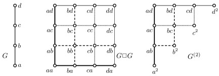
Figure 1: A graph $G$, the Cartesian square $G^{2}=G\Box G$, and the reduced power $G^{(2)}$. For each $x\in V(G)$, the vertices $\{xv\mid v\in V(G)\}$ induce a subgraph $Gx\cong G$ of $G^{(2)}$. These subgraphs are shown dashed, dotted and solid in $G^{(2)}$. Note $Gx$ and $Gy$ intersect precisely at vertex $xy$ if $x\neq y$.

As each monomial $xy$ corresponds uniquely to the $2$-multiset $\{x,y\}$ of vertices of $G$, we can also define the reduced power $G^{(2)}$ as follows. Its vertices are the $2$-multisets of vertices of $G$, with two multisets being adjacent precisely if they agree in one element, and the other elements are adjacent in $G$.

In general, higher reduced powers $G^{(k)}$ can be understood as follows. Suppose $V(G)=\{a_{1},a_{2},\ldots,a_{v}\}$. Any vertex of $G^{(k)}$ is the $S_{k}$-orbit of some $x=(x_{1},x_{2},\ldots,x_{k})\in V(G^{k})$. For each index $1\leq i\leq v$, say $x$ has $n_{i}\geq 0$ coordinates equal to $a_{i}$. Then $\sum_{i=1}^{v}n_{i}=k$, and the $S_{k}$-orbit of $x$ consists precisely of those $k$-tuples in $V(G^{k})$ having $n_{i}$ coordinates equal to $a_{i}$, for $1\leq i\leq v$. This orbit — this vertex of $G^{(k)}$ — can then be identified with either the degree-$k$ monomial

$$a_{1}^{n_{1}}a_{2}^{n_{2}}\cdots a_{v}^{n_{v}},$$

or with the $k$-multiset

$$\{\,\underbrace{a_{1},a_{1},\ldots,a_{1}}_{n_{1}}\mid\underbrace{a_{2},a_{2},\ldots,a_{2}}_{n_{2}}\mid\ldots\;\ldots\mid\underbrace{a_{v},a_{v},\ldots,a_{v}}_{n_{v}}\,\},$$ (1)

where $v-1$ dividing bars are inserted for clarity. We will mostly use the monomial notation for $V(G^{(k)})$, but will also employ the multiset phrasing when convenient. Let us denote the set of monic monomials of degree $k$, with indeterminates $V(G)$, as $M_{k}(G)$, with $M_{0}(G)=\{1\}$. The above, together with the definition of the Cartesian product, yields the following.

Definition 1.

For a graph $G$ with vertex set $\{a_{1},a_{2},\ldots,a_{v}\}$, the reduced $\boldsymbol{k}$th power $G^{(k)}$ is the graph whose vertices are the monomials $a_{1}^{n_{1}}a_{2}^{n_{2}}\cdots a_{v}^{n_{v}}\in M_{k}(G)$. For edges, if $a_{i}a_{j}$ is an edge of $G$, and $f(a_{1},a_{2},\ldots a_{v})\in M_{k-1}(G)$, then $a_{i}f(a_{1},a_{2},\ldots,a_{v})$ is adjacent to $a_{j}f(a_{1},a_{2},\ldots,a_{v})$.

Figure 2 shows the three-cycle $G=C_{3}$ and its reduced second and third powers. Figure 3 shows the five-cycle and its reduced second and third powers.

The reduced power $G^{(k)}$ is not to be confused with the symmetric power of $G$, for which each vertex represents a $k$-subset of $V(G)$, and two $k$-subsets are joined if and only if their symmetric difference is an edge of $G$ [17, 18].

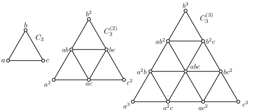
Figure 2: The three-cycle $C_{3}$ and its second and third reduced powers $C_{3}^{(2)}$ and $C_{3}^{(3)}$.

The multiset notation (1) gives a quick formula for the number of vertices of reduced $k$th powers. This presentation describes the multiset as a list of length $k+v-1$ involving $k$ symbols $a_{i}$, $1\leq i\leq k$, and $v-1$ separating bars. We can count the multisets by choosing $k$ slots for the $a_{i}$’s and filling in the remaining slots with bars. Therefore, when $|V(G)|=v$,

$$\left|V\big{(}G^{(k)}\big{)}\right|=\binom{k+v-1}{k}.$$ (2)

The number of vertices in $G^{k}$ that are identified with vertex $a_{1}^{n_{1}}a_{2}^{n_{2}}\cdots a_{v}^{n_{v}}\in V(G^{(k)})$ in the quotient $G^{(k)}=G^{k}/S_{k}$ is given by the multinomial coefficient $\binom{k}{n_{1}\;n_{2}\;\ldots\;n_{v}}$ .

Definition 1 says that for each edge $a_{i}a_{j}$ of $G$, and for each monomial $f\in M_{k-1}(G)$, there is an edge of $G^{(k)}$ from $a_{i}f$ to $a_{j}f$. Because there are $\binom{k+m-2}{k-1}$ such monomials $f$,

$$\left|E\big{(}G^{(k)}\big{)}\right|=|E(G)|\cdot\binom{k+v-2}{k-1}.$$ (3)

3 Reduced graph powers as configuration spaces

The reduced power $G^{(k)}$ is the transition graph of the contracted master Markov chain for $k$ identical and indistinguishable $v$-state automata, each with transition graph $G$. Consequently, an intuitive way of envisioning $G^{(k)}$ is to imagine it as a configuration space in which $k$ indistinguishable tokens are placed on the vertices of $G$, so that any vertex can hold up to $k$ tokens. The monomial $a_{1}^{n_{1}}a_{2}^{n_{2}}\cdots a_{v}^{n_{v}}$ then represents the configuration in which $n_{i}$ tokens are placed on each vertex $a_{i}$. Two configurations are adjacent if one can be transformed to the other by moving a single token along an edge of $G$ to an adjacent vertex. In this way $G^{(k)}$ is interpreted as the space of all such configurations. See [19] for a related construction in which no vertex can hold more than one token.

The reduced power $G^{(k)}$ may also be interpreted the reachability graph for a fundamental class of stochastic Petri nets with $k$ tokens, $v=|V(G)|$ places, and $2|E(G)|$ flow relations (directed arcs) between places [20, 21]. The arc from place $a_{i}$ (origin) to place $a_{j}$ (destination) has firing rate $n_{i}q_{ij}$ given by the product of transition rate $q_{ij}$ and the number $n_{i}$ of tokens in the origin place. That is, the $a_{i}\rightarrow a_{j}$ firing time is the minimum of $n_{i}$ exponentially distributed random variables with expectation $1/q_{ij}$. The $a_{i}\rightarrow a_{j}$ firing rate per token will be denoted $q_{ij}[a_{1}^{n_{1}}a_{2}^{n_{2}}\cdots a_{v}^{n_{v}}]$ when it is a function of the global state (token configuration) of the stochastic Petri net.

The token interpretation can be helpful in deducing properties of reduced powers, such as the following.

Proposition 1.

The vertex $a_{1}^{n_{1}}a_{2}^{n_{2}}\cdots a_{v}^{n_{v}}$ of $G^{(k)}$ has degree

$$\deg\big{(}a_{1}^{n_{1}}a_{2}^{n_{2}}\cdots a_{v}^{n_{v}}\big{)}=\sum_{n_{i}\geq 1}\deg_{G}(a_{i}).$$

Proof.

The configuration $a_{1}^{n_{1}}a_{2}^{n_{2}}\cdots a_{v}^{n_{v}}$ can be transformed to an adjacent configuration only by moving a token on some vertex $a_{i}$ (with $n_{i}\geq 1$) to an adjacent vertex. ∎

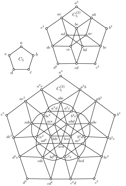
Figure 3: The five-cycle $C_{5}$ and its second and third reduced powers $C_{5}^{(2)}$ and $C_{5}^{(3)}$.

4 Cycle bases and minimum cycle bases

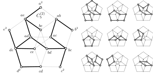
Figure 4: A spanning tree $T$ of $G=C_{5}^{(2)}$. The set $S=E(G)-E(T)$ has $\beta(G)=25-15+1=11$ edges. For each $e\in S$, let $C_{e}$ be the unique cycle in $T+e$. The set $\{C_{e}\ |\ e\in S\}$ is a cycle basis for $G$, but not a minimum cycle basis (see Figure 5).

Here we quickly review the fundamentals of cycle spaces and bases. The following is condensed from Chapter 29 of [16].

For a graph $G$, its edge space $\mathscr{E}(G)$ is the power set of $E(G)$ viewed as a vector space over the two-element field $\mathbb{F}_{2}=\{0,1\}$, where the zero vector is $0=\emptyset$ and addition is symmetric difference. Any vector $X\in\mathscr{E}(G)$ is viewed as the subgraph of $G$ induced on $X$, so $\mathscr{E}(G)$ is the set of all subgraphs of $G$ without isolated vertices. Thus $E(G)$ is a basis for $\mathscr{E}(G)$, and $\dim(\mathscr{E}(G))=|E(G)|$. The vertex space $\mathscr{V}(G)$ of $G$ is the power set of $V(G)$ as a vector space over $\mathbb{F}_{2}$. It is the set of all edgeless subgraphs of $G$ and its dimension is $|V(G)|$.

We define a linear boundary map $\delta_{G}:\mathscr{E}(G)\to\mathscr{V}(G)$ by declaring that $\delta_{G}(xy)=x+y$ on the basis $E(G)$. The subspace $\mathscr{C}(G)=\ker(\delta_{G})$ is called the cycle space of $G$. It contains precisely the subgraphs in $\mathscr{E}(G)$ whose vertices all have even degree (that is, the Eulerian subgraphs). Because every such subgraph can be decomposed into edge-disjoint cycles, each in $\mathscr{C}(G)$, we see that $\mathscr{C}(G)\subseteq$ $\mathscr{E}(G)$ is spanned by the cycles in $G$.

The dimension of $\mathscr{C}(G)$, denoted $\beta(G)$, is called the (first) Betti number of $G$. If $G$ is connected, the rank theorem applied to $\delta_{G}$ yields

$$\beta(G)=|E(G)|-|V(G)|+1.$$ (4)

A basis for the cycle space is called a cycle basis. To make a cycle basis of a connected graph $G$, take a spanning tree $T$, so the set $S=E(G)-E(T)$ has $|E(G)|-|V(G)|+1=\beta(G)$ edges. For each $e\in S$, let $C_{e}$ be the unique cycle in $T+e$. Then the set $\mathscr{B}=$ $\{C_{e}\ |\ e\in S\}$ is linearly independent. As $\mathscr{B}$ has cardinality $\beta(G)$, it is a basis (see Figure 4).

The elements of a cycle basis are naturally weighted by their number of edges. The total length of a cycle basis $\mathscr{B}$ is the number $\ell(\mathscr{B})=\sum_{C\in\mathscr{B}}|C|$. A cycle basis with the smallest possible total length is called a minimum cycle basis, or MCB.

The cycle space is a weighted matroid where each element $C$ has weight $|C|$. Hence the Greedy Algorithm [22] always terminates with an MCB: Begin with $\mathscr{M}=\emptyset$; then append shortest cycles to it, maintaining independence of $\mathscr{M}$, until no further shortest cycles can be appended; then append next-shortest cycles, maintaining independence, until no further such cycles can be appended; and so on, until $\mathscr{M}$ is a maximal independent set. Then $\mathscr{M}$ is an MCB.

Here is our primary criterion for determining if a cycle basis is an MCB. (See Exercise 29.4 of [16].)

Proposition 2.

A cycle basis $\mathscr{B}$ $=$ $\{B_{1},B_{2},\ldots,B_{\beta(G)}\}$ for a graph $G$ is an MCB if and only if every $C$ $\in$ $\mathscr{C}(G)$ is a sum of basis elements whose lengths do not exceed $|C|$.

For graphs $G$ and $H$, a weak homomorphism $\varphi:G\to H$ is a map $\varphi:V(G)\to V(H)$ having the property that for each $xy$ of $G$, either $\varphi(x)\varphi(y)$ is an edge of $H$, or $\varphi(x)=\varphi(y)$. Such a map induces a linear map $\varphi^{*}:\mathscr{E}(G)\to\mathscr{E}(H)$ defined on the basis $E(G)$ as $\varphi^{*}(xy)=\varphi(x)\varphi(y)$ provided $\varphi(x)\neq\varphi(y)$, and $\varphi^{*}(xy)=0$ otherwise. Similarly we define $\varphi_{V}^{*}:\mathscr{V}(G)\to\mathscr{V}(H)$ as $\varphi_{V}^{*}(x)=\varphi(x)$ on the basis $V(G)$. Thus we have the following commutative diagram. (Check it on the basis $E(G)$.)

From this, $\varphi^{*}$ restricts to a map $\mathscr{C}(G)\to\mathscr{C}(H)$ on cycle spaces, because if $C\in\mathscr{C}(G)$, then $\delta_{G}(C)=0$, whence $\delta_{H}\varphi^{*}(C)=\varphi_{V}^{*}\delta_{G}(C)=0$, meaning $\varphi^{*}(C)\in\ker(\delta_{H})=$ $\mathscr{C}(H)$. Certainly if $\varphi$ is a graph isomorphism, then $\varphi^{*}$ is a vector space isomorphism.

Of special interest will be the projections $p_{i}:G^{k}\to G$, where $p_{i}(x_{1},x_{2},\ldots,x_{k})=x_{i}$. These are weak homomorphisms and hence induce linear maps $p_{i}^{*}:\mathscr{C}(G^{k})\to\mathscr{C}(G)$.

Another important map is the natural projection $\eta:G^{k}\to G^{(k)}$ sending each $k$-tuple $x=(x_{1},x_{2},\ldots,x_{k})$ to the monomial representing the $S_{k}$-orbit containing $x$. This map $\eta^{*}$ also is a weak homomorphism, inducing a linear map $\eta^{*}:\mathscr{C}(G^{k})\to\mathscr{C}(G^{(k)})$.

Lemma 1.

If $G$ is connected, the map $\eta^{*}:\mathscr{C}(G^{k})\to\mathscr{C}(G^{(k)})$ is surjective.

Proof.

Because any element of $\mathscr{C}(G^{(k)})$ is an edge-disjoint union of cycles, it suffices to show that any cycle $C=f_{0}f_{1}\cdots f_{n}f_{0}\in\mathscr{C}(G^{(k)})$ equals $\eta^{*}(C^{\prime})$ for some $C^{\prime}\in\mathscr{C}(G^{k})$. For each index $i$, let $x_{i}y_{i+1}\in E(G^{k})$ be an edge for which $\eta^{*}(x_{i}y_{i+1})=\eta(x_{i})\eta(y_{i+1})=f_{i}f_{i+1}$. (Each $x_{i}$, $y_{i}$ is a $k$-tuple, and index arithmetic is modulo $n$.) Note that $\eta(x_{i})=\eta(y_{i})$, meaning $x_{i}$ and $y_{i}$ are in the same $S_{k}$-orbit, that is, $y_{i}$ equals $x_{i}$ with its coordinates permuted.

We will argue that each pair $y_{i}$, $x_{i}$ can be joined by a path $P_{i}$ in $G^{k}$, with $\eta^{*}(P_{i})=0$. This will prove the lemma because then

$$C^{\prime}=P_{0}+x_{0}y_{1}+P_{1}+x_{1}y_{2}+P_{2}+\ldots+P_{n}+x_{n}y_{0}\;\in\;\mathscr{C}(G^{k})$$

satisfies $\eta^{*}(C^{\prime})=C$.

Consider two vertices $(\ldots a\ldots b\ldots)$ and $(\ldots b\ldots a\ldots)$ of $G^{k}$ that are identical except for the transposition of two coordinates $a$ and $b$. Take a path $a=v_{0}v_{1}\cdots v_{q}=b$ from $a$ to $b$ in $G$. Now form the following two paths in $G^{k}$

$$\begin{array}[]{ccl}Q&=&(\ldots a\ldots b\ldots)(\ldots v_{1}\ldots b\ldots)(\ldots v_{2}\ldots b\ldots)\ldots(\ldots b\ldots b\ldots)\\ R&=&(\ldots b\ldots a\ldots)(\ldots b\ldots v_{1}\ldots)(\ldots b\ldots v_{2}\ldots)\ldots(\ldots b\ldots b\ldots).\end{array}$$

Concatenation of $Q$ with the reverse of $R$ is a path from $(\ldots a\ldots b\ldots)$ to $(\ldots b\ldots a\ldots)$. Moreover $\eta^{*}(Q+R)=0$ because the images of the $j$th edges of $Q$ and $R$ are always equal; hence the edges cancel in pairs. As $y_{i}$ and $x_{i}$ differ only by a sequence of transpositions of their coordinates, the above construction can be used to build up a path $P_{i}$ from $y_{i}$ to $x_{i}$ with $\eta(P_{i})=0$. ∎

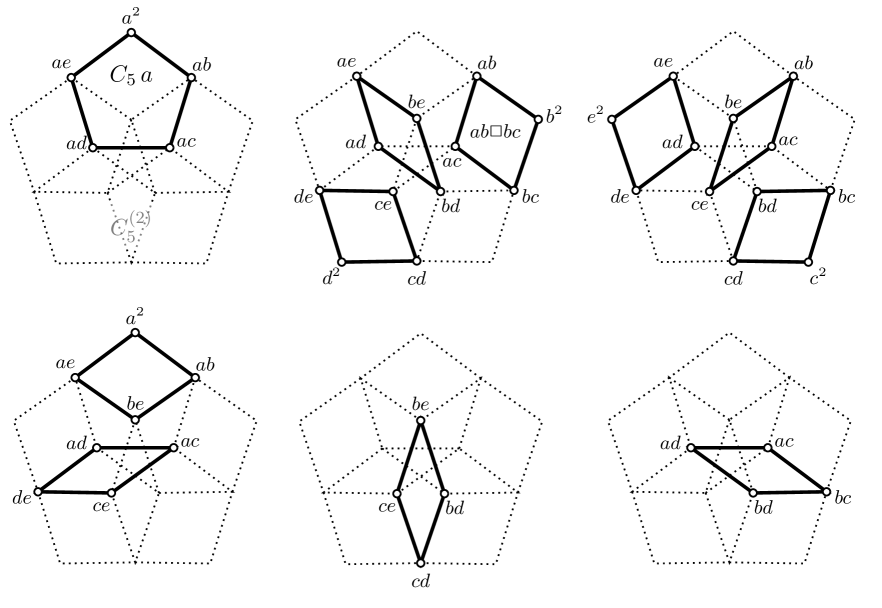
Figure 5: The union $\{C_{5}a\}\cup\mathscr{B}$ is an MCB for $\mathscr{C}(C_{5}^{(2)})=\mathscr{C}(C_{5}\,a)\,\bigoplus\,\mathscr{S}(C_{5}^{(2)})$.

We have seen that the projections $p_{i}:G^{k}\to G$ induce linear maps $\mathscr{C}(G^{k})\to\mathscr{C}(G)$. But there seems to be no obvious way of defining a projection $G^{(k)}\to G$. Still, it is possible to construct a natural linear map $p^{*}:\mathscr{C}(G^{(k)})\to\mathscr{C}(G)$. To do this, recall that any edge of $G^{(k)}$ has form $af\;bf$ where $ab\in E(G)$ and $f\in M_{k-1}(G)$. We begin by defining $p^{*}$ on the edge space. Put $p^{*}(af\;bf)=ab$ for each edge $af\;bf$ in the basis $E(G^{(k)})$ and extend linearly to a map $p^{*}:\mathscr{E}(G^{(k)})\to\mathscr{E}(G)$. Note that $\sum_{i=1}^{k}p_{i}^{*}=p^{*}\circ\eta^{*}$. (Confirm it by checking it on the basis $E(G^{k})$ of $\mathscr{E}(G^{k})$.) Now, if $X\in\mathscr{C}(G^{(k)})$, then Lemma 1 guarantees $X=\eta^{*}(Y)$ for some $Y$ in the cycle space of $G^{k}$. Then $p^{*}(X)=p^{*}(\eta^{*}(Y))=\sum_{i=1}^{k}p_{i}^{*}(Y)\in\mathscr{C}(G)$.

We now have a linear map $p^{*}:\mathscr{C}(G^{(k)})\to\mathscr{C}(G)$ for which $p^{*}(af\;bf)=ab$.

5 Decomposing the cycle space of a reduced power

This section explains how to decompose the cycle space of a reduced power into the direct sum of particularly simple subspaces.

To begin, notice that if $f$ is a fixed monomial in $M_{k-1}(G)$, then there is an embedding $G\to G^{(k)}$ defined as $x\mapsto xf$. Let us call the image of this map $Gf$. Notice that $Gf$ is an induced subgraph of $G^{(k)}$ and is isomorphic to $G$.

Proposition 3.

For any fixed $f\in M_{k-1}(G)$, we have $\mathscr{C}(G^{(k)})=\mathscr{C}(Gf)\bigoplus\ker(p^{*})$.

Proof.

Consider the map $p^{*}:\mathscr{C}(G^{(k)})\to\mathscr{C}(G)$. Its restriction $\mathscr{C}(Gf)\to\mathscr{C}(G)$ is a vector space isomorphism. The proof now follows from elementary linear algebra. ∎

Next we define a special type of cycle in a reduced power. Given distinct edges $ab$ and $cd$ of $G$ and any $f\in M_{k-2}(G)$, we have a square in $G^{(k)}$ with vertices $acf,bcf,bdf,adf$. Let us call such a square a Cartesian square, and denote it as $(ab\Box cd)f$. See Figure 6.

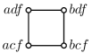
Figure 6: A Cartesian square $(ab\Box cd)f$ in $G^{(k)}$ with $k\geq 2$.

We regard this as a cycle in the cycle space; it is the subgraph of $G^{(k)}$ that is precisely the sum of edges $acf\,bcf+bcf\,bdf+bdf\,adf+adf\,acf.$ (Observe that this sum is zero if and only if $ab=cd$.) We remark that although a subgraph $Gf$ may have squares, they are not Cartesian squares because they do not have the form specified above. Define the square space $\mathscr{S}(G^{(k)})$ to be the subspace of $\mathscr{C}(G^{(k)})$ that is spanned by the Cartesian squares.

If $S$ is a Cartesian square, then $p^{*}(S)=0$, so $\mathscr{S}(G^{(k)})\subseteq\ker(p^{*})$. In the remainder of the paper we will show that in fact $\mathscr{S}(G^{(k)})=\ker(p^{*})$, so that Proposition 3 gives $\mathscr{C}(G^{(k)})=\mathscr{C}(Gf)\bigoplus\mathscr{S}(G^{(k)})$. Simultaneously we will craft a simple MCB for $G^{(k)}$ by concatenating MCBs of $\mathscr{C}(Gf)$ and $\mathscr{S}(G^{(k)})$. See Figure 5 for an example.

6 Cycle bases for reduced powers

This section describes a simple cycle basis for the reduced $k$th power of a graph $G$. If $G$ has no triangles, this cycle basis will be an MCB. (We do not consider MCBs in the cases that $G$ has triangles because the applications we have in mind do not involve such situations. Constructing MCBs when $G$ has triangles would be an interesting research problem.)

Let $G$ be a connected graph with $v$ vertices and $e$ edges. Recall that by Equations (2) and (3), the graph $G^{(k)}$ has $\binom{k+v-1}{k}$ vertices, identified with the monomials $M_{k}(G)$, and $e\binom{k+v-2}{k-1}$ edges. Thus any cycle basis has dimension

$$\beta(G^{(k)})=e\binom{k+v-2}{k-1}-\binom{k+v-1}{k}+1.$$ (5)

We first examine the square space. Any pair of distinct edges $ab$ and $cd$ of $G$ corresponds to a Cartesian square $(ab\Box cd)f$, where $f\in M_{k-2}(G)$, so there are $\binom{e}{2}\binom{k+v-3}{k-2}$ such squares. But this set of squares may not be independent. Our first task will be to construct a linearly independent set of Cartesian squares.

To begin, put $V(G)=\{a_{1},a_{2},\ldots,a_{v}\}$. Let $T$ be a rooted spanning tree of $G$ with root $a_{1}$, and arrange the indexing so its order respects a breadth-first traversal of $T$, that is, for each $i$ the vertex $a_{i}$ is not closer to the root than any $a_{j}$ for which $j<i$ (see Figure 7).

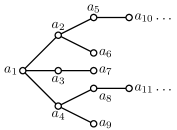
Figure 7: A rooted spanning tree $T$ of $G$ with $V(G)=\{a_{1},a_{2},\ldots,a_{v}\}$, root $a_{1}$, and indexing that respects a breadth-first traversal of $T$.

With this labeling, any edge of $T$ is uniquely determined by its endpoint $a_{j}$ that is furthest from the root. For each $2\leq i\leq v$, let $e_{j}$ be the edge of $T$ that has endpoints $a_{i}$ and $a_{j}$, with $a_{j}$ further from the root than $a_{i}$. Let $M_{k-2}(a_{1},a_{2},\ldots a_{j})$ denote the monic monomials of degree $k-2$ in indeterminates $a_{1},a_{2},\ldots,a_{j}$, with $1\leq j\leq v$. Define the following sets of Cartesian squares in $G^{(k)}$.

$$\Upsilon = \left\{(e_{i}\Box e_{j})f\mid 2\leq i<j\leq v,f\in M_{k-2}(a_{1},a_{2},\ldots,a_{j})\right\},$$

$$\Omega = \left\{(a_{\ell}a_{m}\Box e_{j})f\mid a_{\ell}a_{m}\in E(G)\!-\!E(T),2\leq j\leq v,f\in M_{k-2}(a_{1},a_{2},\ldots,a_{j})\right\}.$$

Shortly we will show that $\Upsilon\cup\Omega$ is linearly independent. But first a few quick informal words about why we would expect this to be the case. Suppose $k\geq 3$ and take three distinct edges $a_{i}a_{j}$, $a_{\ell}a_{m}$ and $a_{p}a_{q}$ in $G$, and let $f\in M_{k-3}(G)$. Figure 8 indicates that these edges result in a cube in the $k$th reduced power. Each of the six square faces of this cube is in the square space. But the faces are dependent because any one of them is a sum of the others. Call a square face such as $(a_{i}a_{j}\Box a_{\ell}a_{m})a_{q}f\,$ a “top square” of a cube if the monomial $a_{q}f$ involves an indeterminate $a_{t}$ with $t>\max\{i,j,\ell,m\}$. Sets $\Upsilon$ and $\Omega$ are constructed so as to contain no top squares.

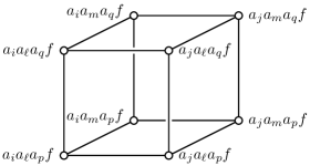
Figure 8: A Cartesian cube $(a_{i}a_{j}\Box a_{\ell}a_{m}\Box a_{p}a_{q})f$ in the reduced power $G^{(k)}$.

(A configuration of the type illustrated in Figure 8 may not always be a cube in the combinatorial sense. The reader is cautioned that if $a_{i}a_{j}$, $a_{\ell}a_{m}$ and $a_{p}a_{q}$ are the edges of a triangle in $G$, then two of the diagonally opposite vertices of the “cube” are the same, as in $K_{3}^{(3)}$, shown in Figure 2. Here there is only one cube, which takes the form of a central vertex connected to the six vertices of a hexagon. This will cause no difficulties in what follows, even if we entertain the possibility that $G$ does indeed have triangles.)

There is another kind of dependency that is ruled out in the definition of $\Upsilon$ and $\Omega$, and we now sketch it. First, imagine $G^{2}$. Consider two cycles $A$ and $B$ in $G$ each having exactly one edge not in $T$, say $a_{i}a_{j}$ and $a_{\ell}a_{m}$, respectively. Envision $A\Box B$ is as a torus in $G^{2}$ with square faces, each edge shared by two faces. In adding up all the faces, the edges cancel in pairs, giving $0$, so the squares are dependent. Removing the face $a_{i}a_{j}\Box a_{\ell}a_{m}$ removes the dependency. Such squares $a_{i}a_{j}\Box a_{\ell}a_{m}$ show up in $G^{(2)}f\subseteq G^{(k)}$ as squares $(a_{i}a_{j}\Box a_{\ell}a_{m})f$ with $a_{i}a_{j},a_{p}a_{q}\in E(G)-E(T)$. Sets $\Upsilon$ and $\Omega$ contain no such squares.

Proposition 4.

The set $\mathscr{B}=\Upsilon\cup\Omega$ is linearly independent.

Proof.

We first show that $\Upsilon$ is linearly independent. Let $X=\sum(e_{i}\Box e_{j})f_{n}$ be a sum of elements of $\Upsilon$. Form the forest $F\subseteq T$ consisting of all edges $e_{i}$ and $e_{j}$ that appear as edges of a squares in this sum, and let $ab$ be an edge of $F$ for which $b$ is a leaf. Then any term $(a_{\ell}a_{m}\Box ab)f_{n}$ of the sum is the unique square in the sum containing the edge $a_{\ell}bf_{n}\;a_{m}bf_{n}$. Because no term can cancel this edge, we get $X\neq 0$, so $\Upsilon$ is linearly independent.

To see that $\Omega$ is linearly independent, consider a sum $X=\sum(a_{\ell}a_{m}\Box e_{j})f_{n}$ of squares in $\Omega$. Again form a forest $F\subseteq T$ of the edges $e_{j}$ and let $ab$ be as before. Then any term $(a_{\ell}a_{m}\Box ab)f_{n}$ is the unique square in the sum containing the edge $a_{\ell}bf_{n}\;a_{m}bf_{n}$. Then $X\neq 0$ because no other term in the sum can cancel this edge; hence $\Omega$ is linearly independent.

Now we argue that the spans of $\Upsilon$ and $\Omega$ have zero intersection. By the previous paragraph, any nonzero linear combination of squares in $\Omega$ has edges of form $(a_{\ell}a_{m}\Box ab)f_{n}$, with $a_{\ell}a_{m}\in E(G)-E(T)$. But no linear combination of squares in $\Upsilon$ has such edges. Hence the spans have zero intersection, so $\mathscr{B}$ is linearly independent. ∎

Our next task is to show that $\mathscr{B}$ is actually a basis for the square space. In fact, we will show more: it is also a basis for $\ker(p^{*})$, and $\mathscr{S}(G^{(k)})=\ker(p^{*})$. Our dimension counts will involve finding $|\Upsilon|$ and $|\Omega|$, and for this we use the following formulas. The first is standard; both are easily verified with induction.

$$\binom{r}{r}\,+\,\binom{r+1}{r}\;+\;\binom{r+2}{r}\;+\;\cdots\;+\;\,\binom{r+n}{r} = \,\;\binom{r+n+1}{r+1}$$ (6)

$$0\binom{r}{r}+1\binom{r+1}{r}+2\binom{r+2}{r}+\;\cdots\;+n\binom{r+n}{r} = n\binom{r+n+1}{r+1}-\binom{r+n+1}{r+2}\;\;\;\;\;$$ (7)

Take an edge $e_{j}$ of $T$ with $3\leq j$. From its definition, $\Upsilon$ has $(j-2)\binom{k+j-3}{k-2}$ squares of form $(e_{i}\Box e_{j})f$. We reckon as follows, using Equations (6) and (7) as appropriate.

$$|\Upsilon| = \sum_{j=3}^{v}(j-2)\binom{k+j-3}{k-2}$$ (8)

$$= \sum_{j=1}^{v}(j-2)\binom{k+j-3}{k-2}+1$$

$$= \sum_{j=1}^{v}(j-1)\binom{k+j-3}{k-2}-\sum_{j=1}^{v}\binom{k+j-3}{k-2}+1$$

$$= (v-1)\binom{k+v-2}{k-1}-\binom{k+v-2}{k}-\binom{k+v-2}{k-1}+1$$

$$= (v-1)\binom{k+v-2}{k-1}-\binom{k+v-1}{k}+1.$$

Now, given and edge $e_{j}$ of $T$ with $2\leq j$, the set $\Omega$ has $\beta(G)\binom{k+j-3}{k-2}$ squares of form $(a_{\ell}a_{m}\Box e_{j})f$. Consequently

$$|\Omega| = \beta(G)\sum_{j=2}^{v}\binom{k+j-3}{k-2}$$ (9)

$$= \beta(G)\left(\sum_{j=1}^{v}\binom{k+j-3}{k-2}-1\right)$$

$$= \beta(G)\binom{k+v-2}{k-1}-\beta(G).$$

Proposition 5.

The set $\mathscr{B}=\Upsilon\cup\Omega$ is a basis for the square space of the reduced $k$th power of $G$. Moreover, the square space equals $\ker(p^{*})$.

Proof.

By Proposition 4, the set $\mathscr{B}$ is linearly independent; and it is a subset of the square space by construction. We saw earlier that the square space is a subspace $\ker(p^{*})$. To finish the proof we show that $\ker(p^{*})$ has dimension $|\mathscr{B}|$. By the rank theorem applied to the surjective map $p^{*}:\mathscr{C}(G^{(k)})\to\mathscr{C}(G)$ we have $\dim\ker(\varphi^{*})=\beta(G^{(2)})-\beta(G)$. This with Equations (5), (8) and (9), as well as the fact that $(v-1)+\beta(G)=e$, gives

$$|\mathscr{B}| = |\Upsilon|+|\Omega|$$

$$= (v-1)\binom{k+v-2}{k-1}-\binom{k+v-1}{k}+1+\beta(G)\binom{k+v-2}{k-1}-\beta(G)$$

$$= e\binom{k+v-2}{k-1}-\binom{k+v-1}{k}+1-\beta(G)$$

$$= \beta(G^{(2)})-\beta(G)$$

$$= \dim\ker(p^{*}).$$

Therefore $\mathscr{B}$ is a basis for both $\mathscr{S}(G^{(k)})$ and $\ker(p^{*})$. ∎

If $k=2$, then $\mathscr{B}=\{ab\Box cd\mid ab,cd\in E(G)\}-\{ab\Box cd\mid ab,cd\in E(G)-E(T)\}$, so $|\mathscr{B}|=\binom{e}{2}-\binom{\beta(G)}{2}$. It is interesting to note that if $\beta(G)\leq 1$, then $\binom{\beta(G)}{2}=0$ and $\mathscr{B}$ consists of all squares in the square space; in all other cases it has fewer squares.

We now can establish the main result of this section, namely a construction of an MCB for the reduced $k$th power. Take an $f\in M_{k-1}(G)$. Propositions 3 and 5 say

$$\mathscr{C}(G^{(k)})=\mathscr{C}(Gf)\,\bigoplus\,\mathscr{S}(G^{(k)}).$$ (10)

To any cycle $C=c_{1}c_{2}\ldots c_{n}$ in $G$, there corresponds cycle $Cf=c_{1}f\,c_{2}f\ldots\,c_{n}f$ in $G^{(k)}$.

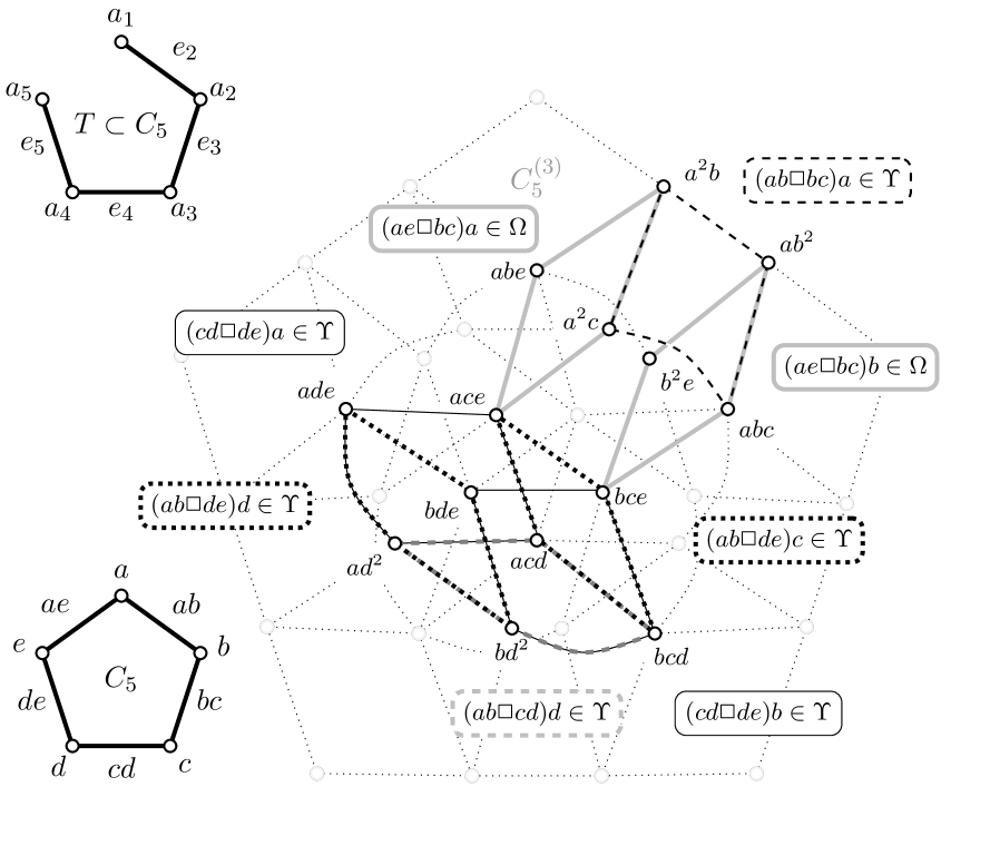
Figure 9: With $T$ as indicated, the sets of squares $\Upsilon$ and $\Omega$ form a basis $\mathscr{B}=\Upsilon\cup\Omega$ of the square space of $C_{5}^{(3)}$. Here $\Upsilon=$ $\{(ab\Box bc)f\mid f\in\{a,b,c\}\}\cup\{(ab\Box cd)f,(bc\Box cd)f\mid f\in\{a,b,c,d\}\}$ $\cup\{(ab\Box de)f,(bc\Box de)f,(cd\Box de)f\mid f\in\{a,b,c,d,e\}\}$. Also $\Omega=$ $\{(ae\Box ab)f\mid f\in\{a,b\}\}\cup\{(ae\Box bc)f\mid f\in\{a,b,c\}\}\cup\{(ae\Box cd)f\mid f\in\{a,b,c,d\}\}\cup\{(ae\Box de)f\mid f\in\{a,b,c,d,e\}\}$. Note $|\Upsilon|=24$ and $|\Omega|=14$. The square $(ab\Box cd)e\notin\mathscr{B}$ is the “top square” of the Cartesian cube $ab\Box cd\Box de$.

Theorem 1.

Take a cycle basis $\mathscr{C}=\{C_{1},C_{2},\ldots,C_{\beta(G)}\}$ for $G$, and let $\mathscr{B}$ be the basis for $\mathscr{S}(G^{(k)})$ constructed above. Fix $f\in M_{k-1}(G)$ and put $\mathscr{C}f=\{C_{1}f,C_{2}f,\ldots,C_{\beta(G)}f\}$. Then $\mathscr{C}f\cup\mathscr{B}$ is a cycle basis for $G^{(k)}$. If $\mathscr{C}$ is an MCB for $G$, and $G$ has no triangles, then this basis is an MCB for $G^{(k)}$.

Proof.

That this is a cycle basis follows immediately from Equation (10).

Now suppose $\mathscr{C}$ is an MCB for $G$, and that $G$ has no triangles. It is immediate that $G^{(k)}$ has no triangles either. The proof is finished by applying Proposition 2. Take any $C\in\mathscr{C}(G^{(k)})$, and write it as

$$C=\sum_{i\in I}G_{i}+\sum_{j\in J}B_{j}\,,$$

where the $G_{i}$ are from $\mathscr{C}f$ and the $B_{j}$ are from $\mathscr{B}$. According to Proposition 2, it suffices to show that $C$ has at least as many edges as any term in this sum. Certainly $C$ is not shorter than any square $B_{j}$ (by the triangle-free assumption). To see that it is not shorter than any $G_{i}$ in the sum, apply $p^{*}$ to the above equation to get

$$p^{*}(C)=\sum_{i\in I}p^{*}(G_{i})\,.$$

Because $p^{*}:\mathscr{C}(Gf)\to\mathscr{C}(G)$ is an isomorphism, the terms $p^{*}(G_{i})$ are part of an MCB for $G$, and thus $|p^{*}(C)|\geq|p^{*}(G_{i})|=|G_{i}|$ for each $i$, by Proposition 2. Also $|C|\geq|p^{*}(C)|$ (as some edges may cancel in the projection) so $|C|\geq|G_{i}|$. ∎

Although Theorem 1 gives a simple MCB for reduced powers of a graph that has no triangles, the constructed basis is definitely not minimum if triangles are present. Several different phenomena account for this. Consider the case $k=2$. First, if $G$ has triangles, then for each vertex $x$ of $G$, the second reduced power contains a copy $Gx$ of $G$. These copies are pairwise edge-disjoint; an MCB would have to capitalize on triangles in each of these copies at the expense of squares in the square space. Moreover, as Figure 2 demonstrates, some of the squares in the square space will actually be sums of two triangles. The figure also shows that for a triangle $\Delta=abc$ in $G$, we do not get just the three triangles $\Delta a$, $\Delta b$ and $\Delta c$, but also a fourth triangle $ab\,bc\,ca$ not belonging to any $Gx$. We do not delve into this problem here.

7 Discussion

We have defined what appears to be a new construction, the $k$th reduced power of a graph, $G^{(k)}$, and have presented a theorem for construction of minimal cycle bases of $G^{(k)}$.

When $G$ is the transition graph for a Markov chain, $G^{(k)}$ is the transition graph for the configuration space of $k$ identical and indistinguishable $v$-state automata with transition graph $G$. Symmetry of model composition allows for interactions among stochastic automata, so long as the transition rates $q_{ij}$ for $i,j\in\{1,2,\cdots,v\}$, $i\neq j$ are constant or functions of the number of automata $n_{\ell}(t)$ in each state, $0\leq n_{\ell}(t)\leq k$, $1\leq\ell\leq v$. $G^{(k)}$ does not pertain if transition rates depend on the state of any particular automaton, $X_{n}(t)\in\{1,2,\cdots,v\}$, $n\in\{1,2,\cdots,k\}$, as this violates indistinguishability.

For concreteness, consider a stochastic automata network composed of three identical automata, each with transition graph $C_{5}$ and generator matrix,

$$Q=\left(\begin{array}[]{ccccc}\diamond&q_{ab}[\cdot]&0&0&q_{ae}\\ q_{ba}&\diamond&q_{bc}&0&0\\ 0&q_{cb}&\diamond&q_{cd}&0\\ 0&0&q_{dc}&\diamond&q_{de}\\ q_{ea}&0&0&q_{ed}&\diamond\\ \end{array}\right)$$ (11)

where $\diamond$’s indicate the values required for zero row sum, $q_{ii}=-\sum_{j\neq i}q_{ij}<0$, and $q_{ab}[\cdot]$ indicates a functional transition rate that depends on the global state of the three automata. Assume constant transition rates $q_{bc}=q_{cd}=q_{de}=q_{ea}=\mu>0$ and $q_{ba}=q_{cb}=q_{dc}=q_{ed}=q_{ae}=\nu>0$. Further assume that the automata may influence one another through the state-dependent transition rate,

$$q_{ab}[\cdot]=\lambda+\alpha\,(n_{a}[\cdot]-1)+\beta\,n_{b}[\cdot]+\gamma\,n_{c}[\cdot]+\delta\,n_{d}[\cdot]+\epsilon\,n_{e}[\cdot],$$ (12)

where $\alpha,\beta,\gamma,\delta,\epsilon\geq 0$ and $[\cdot]$ denotes the global state $a_{1}^{p_{1}}a_{2}^{p_{2}}\cdots a_{v}^{p_{v}}$ that is the functional transition rate’s argument. The transition rate $q_{ab}:M_{k}(a_{1},a_{2},\cdots,a_{v})\rightarrow\mathbb{R}$ is a function of the global state via $n_{\ell}:M_{k}(a_{1},a_{2},\cdots,a_{v})\rightarrow\mathbb{N}$ defined by $n_{\ell}[a_{1}^{p_{1}}a_{2}^{p_{2}}\cdots a_{v}^{p_{v}}]=p_{\ell}$. The three automata are uncoupled when $\alpha,\beta,\gamma,\delta,\epsilon=0$ because this eliminates the dependence of $q_{ab}[\cdot]$ on the global state.

(In this model specification, coupling an isolated component automaton to itself is equivalent to absence of coupling. Because $q_{ab}[\cdot]$ is the rate of an $a\rightarrow b$ transition, $q_{ab}[\cdot]$ is only relevant when the isolated automaton is in state $a$. This functional transition rate has the property that $q_{ab}[a]=\lambda$ when $\alpha,\beta,\gamma,\delta,\epsilon>0$ because $n_{x}[y]=1$ for $x=y$ and 0 otherwise.)

The transition matrix for the master Markov chain $Q^{(3)}$ is defined by the model specification in the previous paragraph. For example, the transition rate from global state $ad^{2}$ to global state $abd$ is $q^{(3)}[ad^{2},abd]=2\mu$ because $n_{d}[ad^{2}]=2$ and $q_{db}=\mu$ is not a function of the global state. Other examples are $q^{(3)}[c^{3},c^{2}d]=n_{c}[c^{3}]q_{cd}=3\nu$, $q[a^{2}c,a^{2}d]=n_{c}[a^{2}c]q_{cd}=\nu$,

$$q^{(3)}[abe,b^{2}e] = n_{a}[abe]q_{ab}[abe]$$

$$= \lambda+\alpha\,(n_{a}[abe]-1)+\beta\,n_{b}[abe]+\gamma\,n_{c}[abe]+\delta\,n_{d}[abe]+\epsilon\,n_{e}[abe]$$

$$= \lambda+\beta+\epsilon$$

$$q^{(3)}[a^{3},a^{2}b] = n_{a}[a^{3}]q_{ab}[a^{3}]$$

$$= 3\left(\lambda+\alpha\,(n_{a}[a^{3}]-1)+\beta\,n_{b}[a^{3}]+\gamma\,n_{c}[a^{3}]+\delta\,n_{d}[a^{3}]+\epsilon\,n_{e}[a^{3}]\right)$$

$$= 3\left(\lambda+2\alpha\right)$$

$$q^{(3)}[a^{2}c,abc] = n_{a}[a^{2}c]q_{ab}[a^{2}c]$$

$$= 2\left(\lambda+\alpha\,(n_{a}[a^{2}c]-1)+\beta\,n_{b}[a^{2}c]+\gamma\,n_{c}[a^{2}c]+\delta\,n_{d}[a^{2}c]+\epsilon\,n_{e}[a^{2}c]\right)$$

$$= 2\left(\lambda+\alpha+\gamma\right).$$

This process of unpacking the model specification yields a master Markov chain with $\eta=\binom{k+v-1}{k}=\binom{3+5-1}{3}=35$ states. The master Markov chain has 210 transition rates $q_{ij}>0$ corresponding (in pairs) to the $5\binom{3+5-2}{3-1}=105$ edges of the master transition graph $C_{5}^{(3)}$.

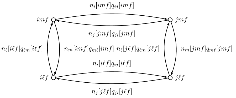
Figure 10: Many cycles of the directed, weighted transition graph for a master Markov chain for $k$ coupled $v$-state automata correspond to Cartesian squares $(ij\Box\ell m)f$ of the minimal cycle basis for the undirected, unweighted transition graph $G^{(k)}$, where $i,j,\ell,m\in\{a_{1},a_{2},\cdots,a_{v}\}$ and $f\in M_{k-2}(a_{1},a_{2},\cdots,a_{v})$.

The construction of minimal cycle bases of $G^{(k)}$ provided by Theorem 1 is especially relevant to stochastic automata networks that arise in physical chemistry and biophysics [23]. For many applications in these domains, the principle of microscopic reversibility requires that the stationary distribution of uncoupled automata satisfying global balance, $\bar{\boldsymbol{\pi}}Q=\boldsymbol{0}$ subject to $\sum_{i}\bar{\pi}_{i}=1$, also satisfies a stronger condition known as detailed balance,

$$\bar{\pi}_{i}\sum_{i\neq j}q_{ij}=\sum_{j\neq i}q_{ji}\bar{\pi}_{j}.$$

In other words, nonequilibrium steady states are forbidden. Markov chains have this property when the transition rates satisfy the Kolmogorov criterion, namely, equality of the product of rate constants in both directions around any cycle in the transition matrix $Q$ [24]. For an isolated automaton with transition graph $C_{5}$ and transition matrix (11), the Komologorov criterion is

$$q_{ab}[a]\,q_{bc}\,q_{cd}\,q_{de}\,q_{ea}=q_{ae}\,q_{ed}\,q_{dc}\,q_{cb}\,q_{ba}.$$ (13)

Substituting the transition rates of the model specification, both those that are constant as well as $q_{ab}[a]=\lambda$ (12), yields the following condition on model parameters,

$$\lambda\mu^{4}=\nu^{5},$$ (14)

that ensures the stationary distribution of an isolated automaton will satisfy detailed balance.

By constructing the minimal cycle basis of $C_{5}^{(3)}$, we may verify that the master Markov chain for three uncoupled automata, each with transition graph $C_{5}$, also exhibits microscopic reversibility under the same parameter constraints.

To see this, recall that the minimal cycle basis of $C_{5}^{(3)}$ has 39 linearly independent cycles. Microscopic reversibility for the master Markov chain for three uncoupled automata requires that, given (14) and $\alpha,\beta,\gamma,\delta,\epsilon=0$, 39 Komolgorov criteria are satisfied, each corresponding to a $C_{i}$ in the MCB for $C_{5}^{(3)}$.

One cycle in the MCB for $C_{5}^{(3)}$ takes the form $C_{5}f$ for fixed $f\in M_{2}(a,b,c,d,e)$. The Kolmogorov criterion for this cycle is

$$n_{a}[af]q_{ab}[af]\cdot n_{b}[bf]q_{bc}[bf]\cdot n_{c}[cf]q_{cd}[cf]\cdot n_{d}[df]q_{de}[df]\cdot n_{e}[ef]q_{ea}[ef]$$

$$=n_{a}[af]q_{ae}[af]\cdot n_{e}[ef]q_{ed}[ef]\cdot n_{d}[df]q_{dc}[df]\cdot n_{c}[cf]q_{cb}[cf]\cdot n_{b}[bf]q_{ba}[bf],$$

where, for typographical efficiency, here and below, we drop the superscripted $(3)$ on the transition rates $q^{(3)}[\cdot,\cdot]$ of $Q^{(3)}$. Canceling identical terms of the form $n_{x}[xf]$ gives

$$q_{ab}[af]\cdot q_{bc}[bf]\cdot q_{cd}[cf]\cdot q_{de}[df]\cdot q_{ea}[ef]=q_{ae}[af]\cdot q_{ed}[ef]\cdot q_{dc}[df]\cdot q_{cb}[cf]\cdot q_{ba}[bf].$$

When this expression is evaluated, the result is another instance of (14), which is satisfied by assumption.

The remaining 38 $C_{i}$ in the MCB for $C_{5}^{(3)}$ are Cartesian squares (see Figure 10) that yield Kolmogorov criteria of the form,

$$n_{i}[imf]q_{ij}[imf]\cdot n_{m}[jmf]q_{m\ell}[jmf]\cdot n_{j}[j\ell f]q_{ji}[j\ell f]\cdot n_{\ell}[i\ell f]q_{\ell m}[i\ell f]$$

$$=n_{m}[imf]q_{m\ell}[imf]\cdot n_{i}[i\ell f]q_{ij}[i\ell f]\cdot n_{\ell}[j\ell f]q_{\ell m}[j\ell f]\cdot n_{j}[jmf]q_{ji}[jmf],$$

where $f\in M_{1}(a,b,c,d,e)$. For $x\neq y$, $n_{x}[xyf]=n_{x}[x]+n_{x}[y]+n_{x}[f]=1+n_{x}[f]$, so this criterion simplifies to

$$(1+n_{i}[f])q_{ij}[imf]\cdot(1+n_{m}[f])q_{m\ell}[jmf]\cdot(1+n_{j}[f])q_{ji}[j\ell f]\cdot(1+n_{\ell}[f])q_{\ell m}[i\ell f]$$

$$=(1+n_{m}[f])q_{m\ell}[imf]\cdot(1+n_{i}[f])q_{ij}[i\ell f]\cdot(1+n_{\ell}[f])q_{\ell m}[j\ell f]\cdot(1+n_{j}[f])q_{ji}[jmf].$$

Canceling identical terms of the form $(1+n_{x}[f])$ gives

$$q_{ij}[imf]\,q_{m\ell}[jmf]\,q_{ji}[j\ell f]\,q_{\ell m}[i\ell f]=q_{m\ell}[imf]\,q_{ij}[i\ell f]\,q_{\ell m}[j\ell f]\,q_{ji}[jmf]$$ (15)

for $(ij\Box\ell m)f\in\mathscr{B}=\Upsilon\cup\Omega$ with $f\in M_{1}(a_{1},a_{2},\ldots,a_{v})$. When the automata are not coupled, $\alpha,\beta,\gamma,\delta,\epsilon=0$, the transition rates are not functions of the global state, and every factor on the left hand side has an equal partner on the right. Consequently, the 38 squares of $\mathscr{B}$ correspond to cycles in $Q^{(3)}$ that satisfy Komolgorov criteria.

We have shown that every cycle in the MCB for $C_{5}^{(3)}$, given by $C_{5}a\cup\mathscr{B}$, corresponds to a cycle in $Q^{(3)}$ that satisfies a Komolgorov criterion. For every cycle in $Q^{(3)}$, there is a representative in the cycle space $\mathscr{C}(C_{5}^{(3)})$ that is a linear combination (over the field $\mathbb{F}_{2}$) of elements of the MCB. It follows that every cycle in the master Markov chain satisfies the Komolgorov criterion. Thus, we conclude that the master Markov chain for three uncoupled automata exhibits microscopic reversibility provided an isolated automaton has this property. This property is expected, and yet important for model verification.

In many applications, it is important to establish whether or not model composition (i.e., the process of coupling the automata) results in a master Markov chain with nonequilibrium steady states, in spite of the fact that an isolated component automaton satisfies detailed balance. Such nonequilibrium steady states may be objects of study or, alternatively, the question may be relevant because the master Markov chain is not physically meaningful when model composition introduces the possibility of nonequilibrium steady states [23].

Our construction of minimal cycle bases of reduced graph powers provides conditions sufficient to ensure that model composition does not introduce nonequilibrium steady states. In general, it is sufficient that (15) hold of every Cartesian square $(ij\Box\ell m)f$ of the MCB for the undirected, unweighted transition graph $G^{(k)}$. In the example under discussion, many of these Komolgorov criteria do not involve the functional transition rate $q_{ab}[\cdot]$; these conditions are satisfied without placing any constraints on the coupling parameters $\alpha,\beta,\gamma,\delta,\epsilon$. The remaining constraints take the form

$$q_{ab}[amf]\,q_{m\ell}[bmf]\,q_{ba}[b\ell f]\,q_{\ell m}[a\ell f]=q_{m\ell}[amf]\,q_{ab}[a\ell f]\,q_{\ell m}[b\ell f]\,q_{ba}[bmf]$$ (16)

for $\ell m\in\{bc,cd,de,ae\}$. The Cartesian squares of concern are elements of the set $\{(ab\Box\ell m)f\mid\ell m\in\{bc,cd,de\}\}\subset\Upsilon$ and $(ae\Box ab)f\in\Omega$. Note that $\ell m\neq ab$ and, consequently, $q_{m\ell}[bmf]=q_{m\ell}[amf]$, $q_{\ell m}[a\ell f]=q_{\ell m}[b\ell f]$ and $q_{ba}[b\ell f]=q_{ba}[bmf]=\nu$. Thus, (16) simplifies to

$$q_{ab}[a\ell f]=q_{ab}[amf]\quad\quad\ell m\in\{bc,cd,de,ae\}.$$ (17)

To see how this requirement constrains the coupling parameters $\alpha,\beta,\gamma,\delta,\epsilon$, we expand both sides of (17) using (12), for example,

$$q_{ab}[a\ell f] = \lambda+\alpha(n_{a}[a\ell f]-1)+\beta n_{b}[a\ell f]+\gamma n_{c}[a\ell f]+\delta n_{d}[a\ell f]+\epsilon n_{e}[a\ell f]$$

$$= \lambda+\alpha n_{a}[\ell f]+\beta n_{b}[\ell f]+\gamma n_{c}[\ell f]+\delta n_{d}[\ell f]+\epsilon n_{e}[\ell f]$$

where we used $n_{a}[a\ell f]=1+n_{a}[\ell f]$. Subtracting both sides of (17) by $\lambda+\alpha n_{a}[f]+\beta n_{b}[f]+\gamma n_{c}[f]+\delta n_{d}[f]+\epsilon n_{e}[f]$ and using $n_{x}[\ell f]=n_{x}[\ell]+n_{x}[f]$ we obtain

$$\alpha n_{a}[\ell]+\beta n_{b}[\ell]+\gamma n_{c}[\ell]+\delta n_{d}[\ell]+\epsilon n_{e}[\ell]=\alpha n_{a}[m]+\beta n_{b}[m]+\gamma n_{c}[m]+\delta n_{d}[m]+\epsilon n_{e}[m]$$

for $\ell m\in\{bc,cd,de,ae\}$. These four equations yield four parameter constraints that ensure detailed balance in the master Markov chain for the three coupled stochastic automata, for example, $\ell m=bc$ gives

$$\alpha n_{a}[b]+\beta n_{b}[b]+\gamma n_{c}[b]+\delta n_{d}[b]+\epsilon n_{e}[b]=\alpha n_{a}[c]+\beta n_{b}[c]+\gamma n_{c}[c]+\delta n_{d}[c]+\epsilon n_{e}[c],$$

which implies that $\beta=\gamma$. Substituting $\ell m=cd$, $de$ and $ae$, we find $\gamma=\delta$, $\delta=\epsilon$ and $\alpha=\epsilon$, respectively. We conclude that $\alpha=\beta=\gamma=\delta=\epsilon$.

In our example, the three automata are coupled when one or more of $\alpha,\beta,\gamma,\delta,\epsilon$ is positive. The analysis of Cartesian squares in the MCB for $C_{5}^{(3)}$ shows that coupling the three automata in the manner specified by (12) will introduce nonequilibrium steady states unless the coupling parameters are equal. This result is intuitive because $\sum_{i}n_{i}[\cdot]=k=3$ and, consequently, equal coupling parameters $\alpha=\beta=\gamma=\delta=\epsilon$ correspond to a functional transition rate that, for every global state, evaluates to the constant $q_{ab}[\cdot]=\lambda+\alpha(k-1)=\lambda+2\alpha$.

The simplicity of this parameter constraint is a consequence of evaluating (15) in the context of the example model specification. In general, the resulting constraints may be more complex and less restrictive. Any choice of model parameters that simultaneously satisfies

$$q_{ij}[imf]\,q_{m\ell}[jmf]\,q_{ji}[j\ell f]\,q_{\ell m}[i\ell f]=q_{m\ell}[imf]\,q_{ij}[i\ell f]\,q_{\ell m}[j\ell f]\,q_{ji}[jmf]$$

for $(ij\Box\ell m)f\in\mathscr{B}=\Upsilon\cup\Omega$ with $f\in M_{k-2}(a_{1},a_{2},\ldots,a_{v})$ are conditions sufficient to ensure that the process of model composition (i.e., coupling $k$ identical and indistinguishable $v$-state automata) does not introduce a violation of microscopic reversibility.

References

- [1] JR Norris. Markov chains. Cambridge University Press, Cambridge, 1997.
- [2] B Plateau and JM Fourneau. A methodology for solving markov models of parallel systems. Journal of Parallel and Distributed Computing, 12:370–387, 1991.
- [3] MF Neuts. Structured stochastic matrices of M/G/1 type and their applications. Probability: Pure and Applied. CRC Press, 2nd edition, 1989.
- [4] DT Gillespie. Stochastic simulation of chemical kinetics. Annual review of physical chemistry, 58:35–55, 2007.
- [5] D Colquhoun and AG Hawkes. A Q-matrix cookbook: how to write only one program to calculate the sigle-channel and macroscopic predictions for any kinetic mechanism. In B Sakmann and E Neher, editors, Single-Channel Recording, pages 589–633. Plenum Press, New York, 1995.
- [6] WJ Stewart. Introduction to the Numerical Solution of Markov Chains. Princeton University Press, Princeton, 1994.
- [7] TM Liggett. Stochastic interacting systems: contact, voter and exclusion processes. A series of comprehensive studies in mathematics. Springer, 1999.
- [8] GF Ball, RK Milne, and GF Yeo. Stochastic models for systems of interacting ion channels. IMA Journal of Medicine and Biology, 17(3):263–293, 2000.
- [9] WJ Richoux and GC Verghese. A generalized influence model for networked stochastic automata. IEEE Transactions on Systems, Man, and Cybernetics - Part A: Systems and Humans, 41(1):10–23, 2011.
- [10] J Campos, S Donatelli, and M Silva. Structured solution of asynchronously communicating stochastic modules. IEEE Trans. Software Eng., 25(2):147–165, 1999.
- [11] A Benoit, P Fernandes, B Plateau, and WJ Stewart. On the benefits of using functional transitions and Kronecker algebra. Perform. Eval., 58(4):367–390, 2004.
- [12] P Buchholz. Hierarchical Markovian models: Symmetries and reduction. Perform. Eval., 22(1):93–110, 1995.
- [13] P Buchholz. Exact and ordinary lumpability in finite Markov chains. Journal of Applied Probability, 31:59–75, 1994.
- [14] A Benoit, L Brenner, P Fernandes, and B Plateau. Aggregation of stochastic automata networks with replicas. Linear Algebra and Its Applications, 386:111–136, 2004.
- [15] O Gusak, T Dayar, and J-M Fourneau. Lumpable continuous-time stochastic automata networks. European Journal of Operational Research, 148(2):436–451, 2003.
- [16] Richard Hammack, Wilfried Imrich, and Sandi Klavžar. Handbook of product graphs. Discrete Mathematics and its Applications (Boca Raton). CRC Press, Boca Raton, FL, second edition, 2011. With a foreword by Peter Winkler.
- [17] A Alzaga, R Iglesias, and R Pignol. Spectra of symmetric powers of graphs and the Weisfeiler-Lehman refinements. Journal of Combinatorial Theory, Series B, 100(6):671–682, 2010.
- [18] K Audenaert, C Godsil, G Royle, and T Rudolph. Symmetric squares of graphs. Journal of Combinatorial Theory, Series B, 97(1):74–90, 2007.
- [19] Ruy Fabila-Monroy, David Flores-Peñaloza, Clemens Huemer, Ferran Hurtado, Jorge Urrutia, and David R. Wood. Token graphs. Graphs Combin., 28(3):365–380, 2012.
- [20] P Buchholz and P Kemper. Hierarchical reachability graph generation for petri nets. Formal Methods in System Design, 21(3):281–315, 2002.
- [21] W Reisig. Understanding Petri Nets: Modeling Techniques, Analysis Methods, Case Studiess. Springer, 2013.
- [22] James G. Oxley. Matroid theory. Oxford Science Publications. The Clarendon Press, Oxford University Press, New York, 1992.
- [23] TL Hill. Free Energy Transduction in Biology and Biochemical Cycle Kinetics. Springer-Verlag, New York, 1989.
- [24] FP Kelly. Reversibility and Stochastic Networks. Cambridge Mathematical Library. Cambridge University Press, Cambridge, 2011.