Geodesic Deviation Equation in $\Lambda$CDM $f(T,\mathcal{T})$ gravity

Abstract

The geodesic deviation equation has been investigated in the framework of $f(T,\mathcal{T})$ gravity, where $T$ denotes the torsion and $\mathcal{T}$ is the trace of the energy-momentum tensor, respectively. The FRW metric is assumed and the geodesic deviation equation has been established following the General Relativity approach in the first hand and secondly, by a direct method using the modified Friedmann equations. Via fundamental observers and null vector fields with FRW background, we have generalized the Raychaudhuri equation and the Mattig relation in $f(T,\mathcal{T})$ gravity. Furthermore, we have numerically solved the geodesic deviation equation for null vector fields by considering a particular form of $f(T,\mathcal{T})$ which induces interesting results susceptible to be tested with observational data.

I Introduction

General Relativity (GR), still known as the general theory of relativity is a geometrical theory of gravitation published by Albert Einstein in 1915 and also a current description of gravitation in modern physics. Relativity General generalizes special relativity and Newton’s laws of gravitation and thus provides an unified description of gravity as a rise property of the geometry of space and time, or at least space-time. In particular, the curvature of space-time is directly related to the energy and momentum generated by presence of matter and radiation in space-time. This interaction between the geometry and the energy-momentum is specified by Einstein’s equations, a system of partial differential equations. One of the most features studied in this successful theory of Einstein (GR) is the Geodesic Deviation Equation (GDE) Misner . Indeed, the relative motion of test particles is one of the important way to get informations on the gravitational field and on the space-time geometry. This motion is described by the Geodesic Deviation Equation . It can be claimed that the GDE is also one of the most important equations in relativity for the fact that it gives a way to step the curvature of space-time. This feature in relativity has been discussed by Szekeres eti25 . The curvature of space-time described by Riemann tensor manifests through the GDE eti20 -eti22 and the relative acceleration of test particules also known under the denomination tidal acceleration. The meaning of GDE in relation with the relative acceleration and tidal forces between two neighboring particles in free fall under the influence of gravity was so stressed for several times by half of the fifties. The importance of GDE for spinless particles was emerged by the authors eti23 ,eti24 . They have notified this importance when they study the gravitational waves and their detection. The GDE provides a graceful tool to explore time-like, space-like and null structures of space-time geometry and we can get, by solving it, the following important relations: the Raychaudhuri equation eti26 , the Mattig relation eti27 and the Pirani equation eti28 .

Actually, the current accelerating Universe was strongly confirmed by several independent experiments such as Radiation of Cosmic Microwave Background (CMBR) Spergel and the Sloan Digital Sky Survey (SDSS) Adelman . This state of Universe is attempted to be explained in the litterature by two approaches. The first approach involves the correction of General Relativity and the second assumes that the Universe is dominated by an antigravity component called dark energy. All these approaches are based on the fundamental theories of gravity namely General Relativity and Tele-parallel Theory equivalent of GR (TEGR)a' and on the modified gravity theories. Severals modified theories have been constructed by modification of GR:( $f(R)$, $f(R,\mathcal{T})$ ma1 -ma6 , $f(G)$ mj1 -mj5 ) where $R$ is the scalar curvature, $\mathcal{T}$ is the trace of energy-momentum tensor and $G$ the Gauss-Bonnet invariant defined by $G=R^{2}-4R_{\mu\nu}R^{\mu\nu}+R_{\mu\nu\lambda\sigma}R^{\mu\nu\lambda\sigma}$. Furthermore, an another approach which in spirit, is similar to the first modification of GR is the so called $f(T)$ theory which is the modified version of TEGR with $T$ the scalar torsion.
Indeed, instead of the connection of Levi-Civi as it is done in GR, $f(T)$ gravity uses the Weitzenbok connection. This theory was introduced for the first time by FerraroFerraro1 in their work on UV modification of GR and inflation. Very soon after and in the context of modern cosmology, Ferraro and Bengochea Ferraro2 considered the same theory to describe dark energy. Other studies can be cited as examples: st1 - st41 . Here, a special attention was tuned to the theory $f(T,\mathcal{T})$ as an extension of the $f(T)$ gravity with $\mathcal{T}$ the trace of energy-momentum tensor. Severals works with interessing results have been developped in this framework sala1 - sala4 .

The GDE has already been studied in $f(R)$ theory eti35 ,eti36 , $f(T)$ theory and also $f(R,\mathcal{T})$ gravity etienne where $R$, $T$ and $\mathcal{T}$ are still the objects defined earlier. Excellent results have been found with these above theories. Our main goal in this present work is to find a new approach to get the GDE in the $f(T,\mathcal{T})$ gravity.

This paper is organised as follow: In Sec II we introduce the gravity $f(T,\mathcal{T})$ and obtain its field equation in cosmology FLRW . The Sec III reminds the GDE in the context of General Relativity and we have extended this study to $f(T,\mathcal{T})$ theory at Sec IV. A conclusion comes naturally to sanction the end of our work in Sec V.

II Generality on $f(T,\mathcal{T})$ gravity within FLRW Cosmology

In Tele-parallel theory, equivalent of General Relativity, the action is constructed by the teleparallel Lagrangian ”scalar torsion $T$ ”. It has modified versions which are the results of the subtitution of scalar torsion in its action by an arbitrary function of the scalar torsion. This approach is similar in spirit to the generalization of the Ricci scalar $R$ in the Einstein-Hilbert action to a function $f(R)$.

This theory and its modified versions used orthonormal tetrads defined on the tangent space at each point of the manifold which is the ordinary space-time. The line element can be written as

$$ds^{2}=g_{\mu\nu}dx^{\mu}dx^{\nu}=\eta_{ij}\theta^{i}\theta^{j}\,,$$ (1)

whose elements can also be expressed as

$$d^{\mu}=e_{i}^{\;\;\mu}\theta^{i};\,\quad\theta^{i}=e^{i}_{\;\;\mu}dx^{\mu}.$$ (2)

Here $\eta_{ij}=diag(1,-1,-1,-1)$ is the Minkowskian metric and $\{e^{i}_{\;\mu}\}$ represent the components of tetrads and satisfy the following identity

$$e^{\;\;\mu}_{i}e^{i}_{\;\;\nu}=\delta^{\mu}_{\nu},\quad e^{\;\;i}_{\mu}e^{\mu}_{\;\;j}=\delta^{i}_{j}.$$ (3)

We recall here Levi-Civita connection used in General Relativity

$$\overset{\circ}{\Gamma}{}_{\;\;\mu\nu}^{\rho}=\frac{1}{2}g^{\rho\sigma}\left(\partial_{\nu}g_{\sigma\mu}+\partial_{\mu}g_{\sigma\nu}-\partial_{\sigma}g_{\mu\nu}\right)\;.$$ (4)

The curvature associated to this connection is not zero while the torsion vanishes. By opposition to this fundamental property of the Levi-Civita connection, the Weizenbock connection which governs tensor relations in Tele-Parallel theory and its modified versions is defined by

$$\Gamma^{\lambda}_{\mu\nu}=e^{\;\;\lambda}_{i}\partial_{\mu}e^{i}_{\;\;\nu}=-e^{i}_{\;\;\mu}\partial_{\nu}e_{i}^{\;\;\lambda}.$$ (5)

With this connection and through the following relations, we get the representations of the fundamental geometrical objects namely the torsion and contorsion in (6) and (8) respectively, from which we determine the tensor $S_{\lambda}^{\;\;\mu\nu}$ in (9)

$$T^{\lambda}_{\;\;\;\mu\nu}=\Gamma^{\lambda}_{\mu\nu}-\Gamma^{\lambda}_{\nu\mu},$$ (6)

which begots

$$K_{\;\;\mu\nu}^{\lambda}\equiv\widetilde{\Gamma}_{\;\mu\nu}^{\lambda}-\overset{\circ}{\Gamma}{}_{\;\mu\nu}^{\lambda}=\frac{1}{2}(T_{\mu}{}^{\lambda}{}_{\nu}+T_{\nu}{}^{\lambda}{}_{\mu}-T_{\;\;\mu\nu}^{\lambda})\;,$$ (7)

where $\overset{\circ}{\Gamma}{}_{\;\;\mu\nu}^{\lambda}$ is by definition the Levi-Civita connection. So

$$K^{\mu\nu}_{\;\;\;\;\lambda}=-\frac{1}{2}\left(T^{\mu\nu}_{\;\;\;\lambda}-T^{\nu\mu}_{\;\;\;\;\lambda}+T^{\;\;\;\nu\mu}_{\lambda}\right)\,\,.$$ (8)

And the tensor $S_{\lambda}^{\;\;\mu\nu}$ is also

$$S_{\lambda}^{\;\;\mu\nu}=\frac{1}{2}\left(K^{\mu\nu}_{\;\;\;\;\lambda}+\delta^{\mu}_{\lambda}T^{\alpha\nu}_{\;\;\;\;\alpha}-\delta^{\nu}_{\lambda}T^{\alpha\mu}_{\;\;\;\;\alpha}\right).$$ (9)

The total contraction of torsion tensor by this latter gives the scalar torsion as

$$T=T^{\lambda}_{\;\;\;\mu\nu}S^{\;\;\;\mu\nu}_{\lambda}$$ (10)

As it has been introduced above, our present investigation will be carried out under the modified theories of Tele-Parallel theory where we replace the scalar torsion in Tele-Parallel action by an arbitrary scalar torsion function, giving the action of these modified versions. Indeed, in the specific case of our present project, the action in a Universe governed by modified Tele-Parallel theory is

$$S=\int e[\frac{T+f(T,\mathcal{T})}{2\kappa^{2}}+\mathcal{L}_{m}]d^{4}x,$$ (11)

where $\kappa^{2}=8\pi G$ is the usual gravitational coupling constant. By varying the action (11) with respect to the tetrads, one gets the following equations of motion sala1 - sala4

$$[\partial_{\xi}(ee^{\rho}_{a}S^{\;\;\sigma\xi}_{\rho})-ee^{\lambda}_{a}S^{\rho\xi\sigma}T_{\rho\xi\lambda}](1+f_{T})+ee^{\rho}_{a}(\partial_{\xi}T)S^{\;\;\sigma\xi}_{\rho}f_{TT}+\frac{1}{4}ee^{\sigma}_{a}(T)$$

$$=-\frac{1}{4}ee^{\sigma}_{a}\Big{(}f(\mathcal{T})\Big{)}-ee^{\rho}_{a}(\partial_{\xi}\mathcal{T})S^{\;\;\sigma\xi}_{\rho}f_{T\mathcal{T}}+f_{\mathcal{T}}\;\Big{(}\frac{e\,\Theta^{\sigma}_{\;\;a}+ee^{\sigma}_{a}\;p}{2}\Big{)}+\frac{\kappa^{2}}{2}e\,\Theta^{\sigma}_{\;\;a}\;,$$ (12)

with $f_{\mathcal{T}}=\partial f/\partial\mathcal{T}$, $f_{T}=\partial f/\partial T$, $f_{T\mathcal{T}}=\partial^{2}f/\partial T\partial\mathcal{T}$, $f_{TT}=\partial^{2}f/\partial T^{2}$ and $\Theta^{\sigma}_{\;\;a}$ the energy-momentum tensor of matter fields.

After some contraction, we can establish the following relations

$$e^{a}_{\nu}e^{-1}\partial_{\xi}(ee^{\rho}_{a}S^{\;\;\sigma\xi}_{\rho})-S^{\rho\xi\sigma}T_{\rho\xi\nu}=-\nabla^{\xi}S_{\nu\xi}^{\;\;\;\;\sigma}-S^{\xi\rho\sigma}K_{\rho\xi\nu}\;,$$ (13)

and

$$G_{\mu\nu}-\frac{1}{2}\,g_{\mu\nu}\,T=-\nabla^{\rho}S_{\nu\rho\mu}-S^{\sigma\rho}_{\;\;\;\;\mu}K_{\rho\sigma\nu}\;.$$ (14)

We transform the field equations Eq. (II) by combining equations Eq. (13) and Eq. (14). We obtain

$$A_{\mu\nu}(1+f_{T})+\frac{1}{4}g_{\mu\nu}\;T=B_{\mu\nu}^{eff},$$ (15)

with

$$A_{\mu\nu}=g_{\sigma\mu}e^{a}_{\nu}[e^{-1}\partial_{\xi}(ee^{\rho}_{a}S^{\;\;\sigma\xi}_{\rho})-e^{\lambda}_{a}S^{\rho\xi\sigma}T_{\rho\xi\lambda}],$$ (16)

$$\qquad=-\nabla^{\sigma}S_{\nu\sigma\mu}-S_{\;\;\;\;\mu}^{\rho\lambda}K_{\lambda\rho\nu}=G_{\mu\nu}-\frac{1}{2}g_{\mu\nu}T,\;$$

$$B_{\mu\nu}^{eff}=S^{\rho}_{\;\;\;\mu\nu}\;f_{T\mathcal{T}}\;\partial_{\rho}\mathcal{T}-S^{\rho}_{\;\;\;\mu\nu}\;f_{TT}\;\partial_{\rho}T-\frac{1}{4}g_{\mu\nu}f+f_{\mathcal{T}}\;\Big{(}\frac{\Theta_{\mu\nu}+g_{\mu\nu}\;p}{2}\Big{)}+\frac{\kappa^{2}}{2}\,\Theta_{\mu\nu}\;.$$

Consequently, we can rewrite the equation Eq. (15) in the following form

$$(1+f_{T})\,G_{\mu\nu}=T_{\mu\nu}^{eff},$$ (17)

where

$$T_{\mu\nu}^{eff}=S^{\rho}_{\;\;\;\mu\nu}\;f_{T\mathcal{T}}\;\partial_{\rho}\mathcal{T}-S^{\rho}_{\;\;\;\mu\nu}\;f_{TT}\;\partial_{\rho}T-\frac{1}{4}g_{\mu\nu}\Big{(}T+f\Big{)}+\frac{T\,g_{\mu\nu}\,f_{T}}{2}+f_{\mathcal{T}}\;\Big{(}\frac{\Theta_{\mu\nu}+g_{\mu\nu}\;p}{2}\Big{)}+\frac{\kappa^{2}}{2}\,\Theta_{\mu\nu}\;.$$ (18)

III Geodesic Deviation Equation in GR

In this section, we revisited briefly the GDE notions in General Relativity. Indeed, in order to explain well the geometrical meaning of Riemann tensor, it would be necessary to look into the behavior of two neighboring geodesics. So, let’s assume two neighboring geodesics $C_{1}$ and $C_{2}$ with affine parameter $\nu$ on a 2-surface $S$ (see fig.1). The field vector $V^{\alpha}=\frac{dx^{\alpha}}{d\nu}$ is the normalized tangent vector of the geodesic $C_{1}$ and $\eta^{\alpha}=\frac{dx^{\alpha}}{ds}$ is the deviation vector of these two geodesics. Therefore, we characterize these geodesics with $x^{\alpha}(\nu,s)$.
Beginning with $\pounds_{{}_{V}}\eta^{\alpha}=\pounds_{{}_{\eta}}V^{\alpha}$ ($[V,\eta]^{\alpha}=0$) which leads to $\nabla_{{}_{V}}\nabla_{{}_{V}}\eta^{\alpha}=\nabla_{{}_{V}}\nabla_{\eta}V^{\alpha}$ and using $\nabla_{{}_{X}}\nabla_{{}_{Y}}Z^{\alpha}-\nabla_{{}_{Y}}\nabla_{X}Z^{\alpha}-\nabla_{{}_{[X,Y]}}Z^{\alpha}=R^{\alpha}\,_{\beta\gamma\delta}Z^{\beta}X^{\gamma}Y^{\delta}$ in which $Y^{\alpha}=\eta^{\alpha}$ and $X^{\alpha}=Z^{\alpha}=V^{\alpha}$, we can obtain the GDE as doing in 3 by

$$\frac{D^{2}\eta^{\alpha}}{D\nu^{2}}=-R^{\alpha}\,_{\beta\gamma\delta}V^{\beta}\eta^{\gamma}V^{\delta}.$$ (19)

Now, we briefly review the research results on the GDE in GR. We use the energy-momentum tensor in a purportedly perfect fluid

$$\Theta_{\mu\nu}=(\rho+p)u_{\alpha}u_{\beta}+pg_{\alpha\beta},$$ (20)

where $\rho$ and $p$ denote respectivily the energy density and the pressure. We recall here that the trace of energy-momentum tensor is given by

$$\mathcal{T}=\rho-3p.$$ (21)

Considering the Einstein field equations in GR (with cosmological constant) given by

$$R_{\mu\nu}-\frac{1}{2}Rg_{\mu\nu}+\Lambda g_{\mu\nu}=\kappa\Theta_{\mu\nu},$$ (22)

we can determinate the Ricci scalar and Ricci tensor as follows

$$R=\kappa(\rho-3p)+4\Lambda,$$ (23)

$$R_{\mu\nu}=\kappa(\rho+p)u_{\alpha}u_{\beta}+\frac{1}{2}[\kappa(\rho-p)+2\Lambda]g_{\mu\nu}.$$ (24)

And then, we determinate the (0-4) Riemann curvature tensor by using Eq.(23) and Eq.(24). It results

$$R_{\alpha\beta\gamma\delta} = \frac{1}{2}(g_{\alpha\gamma}R_{\delta\beta}-g_{\alpha\delta}R_{\gamma\beta}+g_{\beta\delta}R_{\gamma\alpha}-g_{\beta\gamma}R_{\delta\alpha})-\frac{R}{6}(g_{\alpha\gamma}g_{\delta\beta}-g_{\alpha\delta}g_{\gamma\beta})+C_{\alpha\beta\gamma\delta}.$$ (25)

Thus, the right hand side of Eq.(19) becomes

$$R^{\alpha}\,_{\beta\gamma\delta}V^{\beta}\eta^{\gamma}V^{\delta}=\left[\frac{1}{3}(\kappa\rho+\Lambda)\epsilon+\frac{1}{2}\kappa(\rho+p)E^{2}\right]\eta^{\alpha},$$ (26)

where $\epsilon=V^{\alpha}V_{\alpha}$ and $E=-V^{\alpha}u_{\alpha}$. We emphasize here that $\epsilon=(-1,0,1)$, which corresponds to space-like, null and time-like geodesics respectively . The equation Eq.(26) reminds us Pirani equation 2 . We note that by considering null the Weyl tensor, we can extract the Pirani equation for every metric, which makes this equation, an equation giving solutions for space-like, null and timelike congruences ellis . In this work, we generalize these resultats in the framework of $f(T,\mathcal{T})$ gravity applied to the metric.

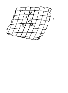
Figure 1: Geodesic Deviation..

IV Geodesics Deviation Equation in $f(T,\mathcal{T})$ gravity

In this section, we establish the GDE in the context of modified $f(T,\mathcal{T})$ gravity. Indeed, we begin our investigation by the Ricci scalar determination from the trace of equation Eq.(15), which leads to

$$R=\frac{-1}{(1+f_{T})}\Bigg{[}S^{\mu}_{\;\;\;\mu\rho}\;f_{T\mathcal{T}}\;\partial^{\rho}\mathcal{T}-S^{\mu}_{\;\;\;\mu\rho}\;f_{TT}\;\partial^{\rho}T+\Big{(}T-f(T,\mathcal{T})\Big{)}+f_{\mathcal{T}}\;\Big{(}\frac{\Theta+4\;p}{2}\Big{)}+\frac{\kappa^{2}}{2}\,\Theta\Bigg{]}.$$ (27)

In order to put out the Ricci tensor in the framework of the $f(T,\mathcal{T})$ gravity, one follows the same way as it has been done in GR by introducing Eq.(27) in Eq.(15). Thus the modified Ricci tensor is presented as follow

$$R_{\mu\nu} = \frac{1}{(1+f_{T})}\Bigg{\{}-g_{\mu\nu}\Big{[}S^{\mu}_{\;\;\;\mu\rho}\;f_{T\mathcal{T}}\;\partial^{\rho}\mathcal{T}-S^{\mu}_{\;\;\;\mu\rho}\;f_{TT}\;\partial^{\rho}T+\Big{(}T-f(T,\mathcal{T})\Big{)}+f_{\mathcal{T}}\;\Big{(}\frac{\Theta+4\;p}{2}\Big{)}$$ (30)

$$+\frac{\kappa^{2}}{2}\,\Theta-\frac{1}{4}(T-f(T,\mathcal{T}))-\frac{f_{\mathcal{T}}\;p}{2}\Big{]}$$

$$+S^{\rho}_{\;\;\;\mu\nu}\;f_{T\mathcal{T}}\;\partial_{\rho}\mathcal{T}-S^{\rho}_{\;\;\;\mu\nu}\;f_{TT}\;\partial_{\rho}T+\frac{(\kappa^{2}+f_{\mathcal{T}})}{2}\,\Theta_{\mu\nu}\Bigg{\}}.$$

If we suppose vanish the Weyl tensor $C_{\alpha\beta\gamma\delta}$, Eq.(25) becomes

$$R_{\alpha\beta\gamma\delta} = \frac{1}{2(1+f_{T})}\Big{[}\frac{(\kappa^{2}+f_{\mathcal{T}})}{2}(g_{\alpha\gamma}\Theta_{\delta\beta}-g_{\alpha\delta}\Theta_{\gamma\beta}+g_{\beta\delta}\Theta_{\gamma\alpha}-g_{\beta\gamma}\Theta_{\delta\alpha})$$ (38)

$$-g_{\mu\nu}\Big{[}S^{\mu}_{\;\;\;\mu\rho}\;f_{T\mathcal{T}}\;\partial^{\rho}\mathcal{T}-S^{\mu}_{\;\;\;\mu\rho}\;f_{TT}\;\partial^{\rho}T+\Big{(}T-f(T,\mathcal{T})\Big{)}+f_{\mathcal{T}}\;\Big{(}\frac{\Theta+4\;p}{2}\Big{)}$$

$$+\frac{\kappa^{2}}{2}\,\Theta-\frac{1}{4}(T-f(T,\mathcal{T}))-\frac{f_{\mathcal{T}}\;p}{2}\Big{]}$$

$$\times(g_{\alpha\gamma}g_{\delta\beta}-g_{\alpha\delta}g_{\gamma\beta})+(g_{\alpha\gamma}D_{\delta\beta}-g_{\alpha\delta}D_{\gamma\beta}+g_{\beta\delta}D_{\gamma\alpha}-g_{\beta\gamma}D_{\delta\alpha})f_{T}$$

$$+(g_{\alpha\gamma}\mathcal{D}_{\delta\beta}-g_{\alpha\delta}\mathcal{D}_{\gamma\beta}+g_{\beta\delta}\mathcal{D}_{\gamma\alpha}-g_{\beta\gamma}\mathcal{D}_{\delta\alpha})f_{T}\Big{]}$$

$$-\frac{1}{6(1+f_{T})}\Bigg{\{}-g_{\mu\nu}\Big{[}S^{\mu}_{\;\;\;\mu\rho}\;f_{T\mathcal{T}}\;\partial^{\rho}\mathcal{T}-S^{\mu}_{\;\;\;\mu\rho}\;f_{TT}\;\partial^{\rho}T+\Big{(}T-f(T,\mathcal{T})\Big{)}+f_{\mathcal{T}}\;\Big{(}\frac{\Theta+4\;p}{2}\Big{)}$$

$$+\frac{\kappa^{2}}{2}\,\Theta-\frac{1}{4}(T-f(T,\mathcal{T}))-\frac{f_{\mathcal{T}}\;p}{2}\Big{]}+S^{\rho}_{\;\;\;\mu\nu}\;f_{T\mathcal{T}}\;\partial_{\rho}\mathcal{T}-S^{\rho}_{\;\;\;\mu\nu}\;f_{TT}\;\partial_{\rho}T$$

$$+\frac{(\kappa^{2}+f_{\mathcal{T}})}{2}\,\Theta_{\mu\nu}\Bigg{\}}(g_{\alpha\gamma}g_{\delta\beta}-g_{\alpha\delta}g_{\gamma\beta}),$$

where

$$D_{\mu\nu}=-S_{\nu\mu\rho}\nabla^{\rho}T\partial_{{}_{T}},$$ (39)

and

$$\mathcal{D}_{\mu\nu}=-S_{\nu\mu\rho}\nabla^{\rho}\,\mathcal{T}\partial_{{}_{\mathcal{T}}}.$$ (40)

Now, we rise the first index $\alpha$ of Riemann tensor in Eq.(25) by a contraction with $V^{\beta}\eta^{\gamma}V^{\delta}$, leading to the following (1, 3)-tensor

$$R^{\alpha}\,_{\beta\gamma\delta}V^{\beta}\eta^{\gamma}V^{\delta} = \frac{1}{2(1+f_{T})}\Big{[}\frac{(\kappa^{2}+f_{\mathcal{T}})}{2}(\delta^{\alpha}_{\gamma}\Theta_{\delta\beta}-\delta^{\alpha}_{\delta}\Theta_{\gamma\beta}+g_{\beta\delta}\Theta^{\alpha}_{\gamma}-g_{\beta\gamma}\Theta^{\alpha}_{\delta})$$ (47)

$$-\Big{[}S^{\mu}_{\;\;\;\mu\rho}\;f_{T\mathcal{T}}\;\partial^{\rho}\mathcal{T}-S^{\mu}_{\;\;\;\mu\rho}\;f_{TT}\;\partial^{\rho}T+\Big{(}T-f(T,\mathcal{T})\Big{)}+f_{\mathcal{T}}\;\Big{(}\frac{\Theta+4\;p}{2}\Big{)}$$

$$+\frac{\kappa^{2}}{2}\,\Theta-\frac{1}{4}(T-f(T,\mathcal{T}))-\frac{f_{\mathcal{T}}\;p}{2}\Big{]}$$

$$\times(\delta^{\alpha}_{\gamma}g_{\delta\beta}-\delta^{\alpha}_{\delta}g_{\gamma\beta})+(\delta^{\alpha}_{\gamma}D_{\delta\beta}-\delta^{\alpha}_{\delta}D_{\gamma\beta}+g_{\beta\delta}D^{\alpha}_{\gamma}-g_{\beta\gamma}D^{\alpha}_{\delta})f_{T}$$

$$+(\delta^{\alpha}_{\gamma}\mathcal{D}_{\delta\beta}-\delta^{\alpha}_{\delta}\mathcal{D}_{\gamma\beta}+g_{\beta\delta}\mathcal{D}^{\alpha}_{\gamma}-g_{\beta\gamma}\mathcal{D}^{\alpha}_{\delta})f_{T}\Big{]}V^{\beta}\eta^{\gamma}V^{\delta}$$

$$-\frac{1}{6(1+f_{T})}\Bigg{\{}-g_{\mu\nu}\Big{[}S^{\mu}_{\;\;\;\mu\rho}\;f_{T\mathcal{T}}\;\partial^{\rho}\mathcal{T}-S^{\mu}_{\;\;\;\mu\rho}\;f_{TT}\;\partial^{\rho}T+\Big{(}T-f(T,\mathcal{T})\Big{)}+f_{\mathcal{T}}\;\Big{(}\frac{\Theta+4\;p}{2}\Big{)}$$

$$+\frac{\kappa^{2}}{2}\,\Theta-\frac{1}{4}(T-f(T,\mathcal{T}))-\frac{f_{\mathcal{T}}\;p}{2}\Big{]}+S^{\rho}_{\;\;\;\mu\nu}\;f_{T\mathcal{T}}\;\partial_{\rho}\mathcal{T}-S^{\rho}_{\;\;\;\mu\nu}\;f_{TT}\;\partial_{\rho}T+\frac{(\kappa^{2}+f_{\mathcal{T}})}{2}\,\Theta_{\mu\nu}\Bigg{\}}$$

$$(g_{\alpha\gamma}g_{\delta\beta}-g_{\alpha\delta}g_{\gamma\beta})V^{\beta}\eta^{\gamma}V^{\delta}.$$

We remark here that Eq.(38) and Eq.(47) are available only if the Weyl tensor is reduced to zero. Otherwise, from Eqs(20) and (38), one points out the following relation

$$R^{\alpha}\,_{\beta\gamma\delta} = \frac{1}{2(1+f_{T})}\Bigg{\{}\frac{(\kappa^{2}+f_{\mathcal{T}})}{2}(\rho+p)(g_{\alpha\gamma}u_{\delta}u_{\beta}-g_{\alpha\delta}u_{\gamma}u_{\beta}+g_{\beta\delta}u_{\gamma}u_{\alpha}-g_{\beta\gamma}u_{\delta}u_{\alpha})-(g_{\alpha\gamma}g_{\delta\beta}-g_{\alpha\delta}g_{\gamma\beta})$$ (51)

$$\times\frac{1}{3}\Big{[}S^{\mu}_{\;\;\;\mu\rho}\;f_{T\mathcal{T}}\;\partial^{\rho}\mathcal{T}-S^{\mu}_{\;\;\;\mu\rho}\;f_{TT}\;\partial^{\rho}T+\Big{(}T-f(T,\mathcal{T})\Big{)}+f_{\mathcal{T}}\;\Big{(}\frac{\Theta+4\;p}{2}\Big{)}+\frac{\kappa^{2}}{2}\,\Theta-\frac{1}{4}(T-f(T,\mathcal{T}))$$

$$-\frac{f_{\mathcal{T}}\;p}{2}\Big{]}$$

$$+(g_{\alpha\gamma}D_{\delta\beta}-g_{\alpha\delta}D_{\gamma\beta}+g_{\beta\delta}D_{\gamma\alpha}-g_{\beta\gamma}D_{\delta\alpha})f_{T}+(g_{\alpha\gamma}\mathcal{D}_{\delta\beta}-g_{\alpha\delta}\mathcal{D}_{\gamma\beta}+g_{\beta\delta}\mathcal{D}_{\gamma\alpha}-g_{\beta\gamma}\mathcal{D}_{\delta\alpha})f_{T}\Bigg{\}}.$$

Under the condition of vector field normalization, we have $V^{\alpha}V_{\alpha}=\epsilon$ and

$$R_{\alpha\beta\gamma\delta}V^{\beta}V^{\delta} = \frac{1}{2(1+f_{T})}\Bigg{\{}\frac{(\kappa^{2}+f_{\mathcal{T}})}{2}(\rho+p)(g_{\alpha\gamma}(u_{\beta}V^{\beta})^{2}-2(u_{\beta}V^{\beta})V_{(\alpha}u_{\gamma)}+\epsilon u_{\alpha}u_{\gamma})$$ (56)

$$-\frac{1}{3}\Big{[}S^{\mu}_{\;\;\;\mu\rho}\;f_{T\mathcal{T}}\;\partial^{\rho}\mathcal{T}-S^{\mu}_{\;\;\;\mu\rho}\;f_{TT}\;\partial^{\rho}T+\Big{(}T-f(T,\mathcal{T})\Big{)}+f_{\mathcal{T}}\;\Big{(}\frac{\Theta+4\;p}{2}\Big{)}$$

$$+\frac{\kappa^{2}}{2}\,\Theta-\frac{1}{4}(T-f(T,\mathcal{T}))-\frac{f_{\mathcal{T}}\;p}{2}\Big{]}$$

$$\times(\epsilon g_{\alpha\gamma}-V_{\alpha}V_{\gamma})+[(g_{\alpha\gamma}D_{\delta\beta}-g_{\alpha\delta}D_{\gamma\beta}+g_{\beta\delta}D_{\gamma\alpha}-g_{\beta\gamma}D_{\delta\alpha})f_{T}]V^{\beta}V^{\delta}$$

$$+[(g_{\alpha\gamma}\mathcal{D}_{\delta\beta}-g_{\alpha\delta}\mathcal{D}_{\gamma\beta}+g_{\beta\delta}\mathcal{D}_{\gamma\alpha}-g_{\beta\gamma}\mathcal{D}_{\delta\alpha})f_{T}]V^{\beta}V^{\delta}\Bigg{\}}.$$

We rise the first index with $\eta^{\gamma}$ and obtain

$$R^{\alpha}\,_{\beta\gamma\delta}V^{\beta}\eta^{\gamma}V^{\delta} = \frac{1}{2(1+f_{T})}\Big{\{}\frac{(\kappa^{2}+f_{\mathcal{T}})}{2}(\rho+p)((u_{\beta}V^{\beta})^{2}\eta^{\alpha}-(u_{\beta}V^{\beta})V^{\alpha}(u_{\gamma}\eta^{\gamma})$$ (62)

$$-(u_{\beta}V^{\beta})u^{\alpha}(V_{\gamma}\eta^{\gamma})+\epsilon u_{\alpha}u_{\gamma}\eta^{\gamma})$$

$$-\frac{1}{3}\Big{[}S^{\mu}_{\;\;\;\mu\rho}\;f_{T\mathcal{T}}\;\partial^{\rho}\mathcal{T}-S^{\mu}_{\;\;\;\mu\rho}\;f_{TT}\;\partial^{\rho}T+\Big{(}T-f(T,\mathcal{T})\Big{)}+f_{\mathcal{T}}\;\Big{(}\frac{\Theta+4\;p}{2}\Big{)}$$

$$+\frac{\kappa^{2}}{2}\,\Theta-\frac{1}{4}(T-f(T,\mathcal{T}))-\frac{f_{\mathcal{T}}\;p}{2}\Big{]}$$

$$\times(\epsilon\eta^{\alpha}-V_{\alpha}(V_{\gamma}\eta^{\gamma}))+[(\delta^{\alpha}_{\gamma}D_{\delta\beta}-\delta^{\alpha}_{\delta}D_{\gamma\beta}+g_{\beta\delta}D^{\alpha}_{\gamma}-g_{\beta\gamma}D^{\alpha}_{\delta})f_{T}]V^{\beta}V^{\delta}\eta^{\gamma}$$

$$+[(\delta^{\alpha}_{\gamma}\mathcal{D}_{\delta\beta}-\delta^{\alpha}_{\delta}\mathcal{D}_{\gamma\beta}+g_{\beta\delta}\mathcal{D}^{\alpha}_{\gamma}-g_{\beta\gamma}\mathcal{D}^{\alpha}_{\delta})f_{T}]V^{\beta}V^{\delta}\eta^{\gamma}\Big{\}}.$$

By using $E=-V_{\alpha}u^{\alpha}$ and $\eta_{\alpha}u^{\alpha}=\eta_{\alpha}V^{\alpha}=0$, Eq. (62) becomes

$$R^{\alpha}\,_{\beta\gamma\delta}V^{\beta}\eta^{\gamma}V^{\delta} = \frac{1}{2(1+f_{T})}\Big{[}\frac{(\kappa^{2}+f_{\mathcal{T}})}{2}(\rho+p)E^{2}-\frac{\epsilon}{3}\Big{(}S^{\mu}_{\;\;\;\mu\rho}\;f_{T\mathcal{T}}\;\partial^{\rho}\mathcal{T}-S^{\mu}_{\;\;\;\mu\rho}\;f_{TT}\;\partial^{\rho}T+\Big{(}T-f(T,\mathcal{T})\Big{)}$$ (66)

$$+f_{\mathcal{T}}\;\Big{(}\frac{\Theta+4\;p}{2}\Big{)}+\frac{\kappa^{2}}{2}\,\Theta-\frac{1}{4}(T-f(T,\mathcal{T}))-\frac{f_{\mathcal{T}}\;p}{2}\Big{)}\Big{]}\eta^{\alpha}$$

$$+\frac{1}{2(1+f_{T})}\Big{[}(\delta^{\alpha}_{\gamma}D_{\delta\beta}-\delta^{\alpha}_{\delta}D_{\gamma\beta}+g_{\beta\delta}D^{\alpha}_{\gamma}-g_{\beta\gamma}D^{\alpha}_{\delta})f_{T}]V^{\beta}V^{\delta}\Big{]}\eta^{\gamma}$$

$$+\frac{1}{2(1+f_{T})}\Big{[}(\delta^{\alpha}_{\gamma}\mathcal{D}_{\delta\beta}-\delta^{\alpha}_{\delta}\mathcal{D}_{\gamma\beta}+g_{\beta\delta}\mathcal{D}^{\alpha}_{\gamma}-g_{\beta\gamma}\mathcal{D}^{\alpha}_{\delta})f_{T}]V^{\beta}V^{\delta}\Big{]}\eta^{\gamma}.$$

In the following section and by make using the FLRW metric whose Weyl tensor is zero; we will use these previous results to obtain the GDE in the framework of $f(T,\mathcal{T})$ gravity, which is of course the equivalent of GDE in GR.

IV.1 GR equivalent method with FLRW background

Here we are interested in studying flat FLRW cosmologies whose metric can be described by,

$$ds^{2}=-dt^{2}+a^{2}(t)\left[\frac{dr^{2}}{1-kr^{2}}+r^{2}d\theta^{2}+r^{2}sin^{2}\theta d\phi^{2}\right].$$ (67)

The Weyl tensor associated to this latter is zero because of the flatness conformal of Universe described by FLRW metric. The non-zero components of tetrads according to the above metric are given by

$$\{e^{a}_{\;\;\mu}\}=diag[1,a,a,a].$$ (68)

The determinant of the matrix (68) is $e=a^{3}$ and the non-zero components of the torsion tensor and contorsion tensor are also given by

$$T^{1}_{\;\;\;01}=T^{2}_{\;\;\;02}=T^{3}_{\;\;\;03}=\frac{\dot{a}}{a},$$ (69)

$$K^{01}_{\;\;\;\;1}=K^{02}_{\;\;\;\;2}=K^{03}_{\;\;\;\;3}=\frac{\dot{a}}{a}.$$ (70)

The non-zero components of the tensor $S^{\;\;\;\mu\nu}_{\alpha}$ are

$$S^{\;\;\;11}_{0}=S^{\;\;\;22}_{0}=S^{\;\;\;33}_{0}=\frac{\dot{a}}{a}.$$ (71)

Therefore, one evaluates the torsion scalar and obtains

$$T=-6H^{2},$$ (72)

where $H=\dot{a}/a$ denotes the Hubble parameter. The normalization of the vector field leads to $V_{\alpha}V^{\alpha}=\epsilon$ and we have also $E=-V_{\alpha}u^{\alpha}$, $\eta_{\alpha}u^{\alpha}=\eta_{\alpha}V^{\alpha}=0$, $\eta_{0}u^{0}=0$. Considering (70) and (71) we find $S^{1}_{10}=S^{2}_{20}=S^{3}_{30}=-2H(t)$. Thus, we can reduce the expression of $R^{\alpha}\,_{\beta\gamma\delta}V^{\beta}\eta^{\gamma}V^{\delta}$ as follows

$$R^{\alpha}\,_{\beta\gamma\delta}V^{\beta}\eta^{\gamma}V^{\delta} = \frac{G}{(1+f_{T})}\left(1+\frac{f_{\mathcal{T}}}{16\pi G}\right)\Bigg{\{}4\pi E^{2}(\rho+\rho_{1}+p+p_{1})$$ (74)

$$+\frac{8\pi\,\epsilon}{3}(\rho+\rho_{1})\Bigg{\}}\eta^{\alpha}$$

with

$$G_{eff}=\frac{G}{(1+f_{T})}\left(1+\frac{f_{\mathcal{T}}}{16\pi G}\right)\,,$$ (75)

$$\rho_{1}=\frac{1}{16\pi G_{eff}(1+f_{T})}\left(f_{\mathcal{T}}p-\frac{1}{2}f-\frac{T}{2}\right)\,,$$ (76)

$$p_{1}=\rho+p-\rho_{1}-\frac{1}{4\pi G_{eff}(1+f_{T})}\left[12H^{2}\dot{H}f_{TT}-f_{T\mathcal{T}}H\left(\dot{\rho}-3\dot{p}\right)\right]\,.$$ (77)

The relation so posed in (74) is the generalized Pirani equation. Now, we can write the GDE in $f(T,\mathcal{T})$ gravity model as following

$$\frac{D^{2}\eta^{\alpha}}{D\nu^{2}} = -\frac{G}{(1+f_{T})}\left(1+\frac{f_{\mathcal{T}}}{16\pi G}\right)\Bigg{\{}4\pi E^{2}(\rho+\rho_{1}+p+p_{1})+\frac{8\pi\,\epsilon}{3}(\rho+\rho_{1})\Bigg{\}}\eta^{\alpha}.$$ (78)

For reasons of homogeneity and isotropy of the metric FLRW, there has been a change in the intensity of the deviation vector $\eta^{\alpha}$ where as in the anisotropic Universe like Bianchi Universe I, the GDE has also induced a change in the direction of the deviation vector as described in cac .

IV.2 Direct method with FLRW background

In this section, we can write the GDE in $f(T,\mathcal{T})$ gravity model by evaluating the LHS of Eq.(74) for $\alpha=r$ as follows

$$R^{r}\,_{\beta\gamma\delta}V^{\beta}\eta^{\gamma}V^{\delta}=R^{r}\,_{t\gamma t}V^{t}\eta^{\gamma}V^{t}+R^{r}\,_{r\gamma r}V^{r}\eta^{\gamma}V^{r}+R^{r}\,_{\theta\gamma\theta}V^{\theta}\eta^{\gamma}V^{\theta}+R^{r}\,_{\phi\gamma\phi}V^{\phi}\eta^{\gamma}V^{\phi}.$$ (79)

Assuming that the Riemann tensor components are not different to zero for FLRW metric in Eq.(67), we can take $\gamma=r$. Indeed, Eq.(79) becames:

$$R^{r}\,_{\beta\gamma\delta}V^{\beta}\eta^{\gamma}V^{\delta}=R^{r}\,_{trt}V^{t}V^{t}\eta^{r}+R^{r}\,_{rrr}~{}g^{rr}V_{r}V^{r}\eta^{r}+R^{r}\,_{\theta r\theta}~{}g^{\theta\theta}V_{\theta}V^{\theta}\eta^{r}+R^{r}\,_{\phi r\phi}~{}g^{\phi\phi}V_{\phi}V^{\phi}\eta^{r}=(-\dot{H}E^{2}+\epsilon H^{2})\eta^{r},$$ (80)

where we have used the following expressions $V^{t}V^{t}=E^{2}$, $V_{i}\eta^{i}=0$, $R^{r}\,_{rrr}=0$, $R^{r}\,_{\theta r\theta}=r^{2}\dot{a}^{2}$, $R^{r}\,_{\phi r\phi}=\dot{a}^{2}r^{2}sin^{2}\theta$ and $R^{r}\,_{ttr}=\frac{\ddot{a}}{a}$. Remark that similar equations are also obtained for $\alpha=\theta$ and $\alpha=\phi$. Considering (II) and (67), we obtain the Friedmann standard equations

$$3H^{2}=8\pi G_{eff}\left(\rho+\rho_{1}\right),$$ (81)

and

$$\dot{H}=-4\pi G_{eff}\left(\rho+p+\rho_{1}+p_{1}\right).$$ (82)

By putting the equations (81) and (82) in equation (80), we can generalize the Pirani equations by a direct approach as

$$R^{\alpha}\,_{\beta\gamma\delta}V^{\beta}\eta^{\gamma}V^{\delta} = \frac{G}{(1+f_{T})}\left(1+\frac{f_{\mathcal{T}}}{16\pi G}\right)\Bigg{\{}4\pi E^{2}(\rho+\rho_{1}+p+p_{1})$$ (84)

$$+\frac{8\pi\,\epsilon}{3}(\rho+\rho_{1})\Bigg{\}}\eta^{\alpha},$$

which leads to the same Geodesic Deviation Equation as in (78). This means that we have found the same results by two different approaches . This result proves the validity of the GDE obtained in the context of $f(T,\mathcal{T})$ gravity.

IV.3 Fundamental observers with FLRW background

Here, we are basing our analysis on the fundamental observers. In this particular case, we interprete $V^{\alpha}$ and $\nu$ (affine parameter) as the four-viscosity of fluid $u^{\alpha}$ and $t$ ( proper time). Since we are performing with temporal geodesics, we have $\epsilon=1$. By constraining the vector field normalization as $E=1$, one gets

$$R^{\alpha}\,_{\beta\gamma\delta}u^{\beta}\eta^{\gamma}u^{\delta}=\frac{4\pi\,G}{(1+f_{T})}\left(1+\frac{f_{\mathcal{T}}}{16\pi G}\right)\Bigg{\{}\frac{\rho+\rho_{1}}{3}+(p+p_{1})\Bigg{\}}\eta^{\alpha}.$$ (85)

We know that if $\eta_{\alpha}=\ell e_{\alpha}$, where $e_{\alpha}$ is parallel propagated along $t$, then the isotropy results in

$$\frac{De^{\alpha}}{Dt}=0,$$ (86)

which induces

$$\frac{D^{2}\eta^{\alpha}}{Dt^{2}}=\frac{d^{2}\ell}{dt^{2}}e^{\alpha}.$$ (87)

By using (19) and (85) we can write

$$\frac{d^{2}\ell}{dt^{2}}=\frac{-4\pi\,G}{(1+f_{T})}\left(1+\frac{f_{\mathcal{T}}}{16\pi G}\right)\Bigg{\{}\frac{\rho+\rho_{1}}{3}+(p+p_{1})\Bigg{\}}\ell.$$ (88)

For the particular case $\ell=a(t)$, equation (88) becames

$$\frac{\ddot{a}}{a}=\frac{-4\pi\,G}{(1+f_{T})}\left(1+\frac{f_{\mathcal{T}}}{16\pi G}\right)\Bigg{\{}\frac{\rho+\rho_{1}}{3}+(p+p_{1})\Bigg{\}}.$$ (89)

This equation is a particular case of the generalized Raychaudhuri equation given in eti20 . Furthermore, from the standard forms of the modified Friedmann equations in $f(T,\mathcal{T})$ gravity model for flat Universe rafael2 , the generalized Raychaudhuri equation above can be obtained. These equations are expressed as follows

$$H^{2} = \frac{8\pi G}{3}\rho-\frac{1}{6}\left(f+12H^{2}f_{T}\right)+f_{\mathcal{T}}\left(\frac{\rho+p}{3}\right),$$ (90)

$$\dot{H} = -\frac{4\pi G\left(1+f_{\mathcal{T}}/8\pi G\right)\left(\rho+p\right)}{1+f_{T}-12H^{2}f_{TT}+H\left(d\rho/dH\right)\left(1-3c_{s}^{2}\right)f_{T\mathcal{T}}}.$$ (91)

Consistency between the modified Friedmann equations in $f(T,\mathcal{T})$ gravity applied to flat Universe rafael2 and the generalized Raychaudhuri equation for flat Universe (89) confirms that the approach followed here, is one of the valid approaches.

IV.4 Null vector fields with FLRW background

In this section, we suppose that vector fields are directed the null past, namely $V^{\alpha}=k^{\alpha},k_{\alpha}k^{\alpha}=0$, for which the Eq.(74) leads to

$$R^{\alpha}\,_{\beta\gamma\delta}k^{\beta}\eta^{\gamma}k^{\delta}=\frac{4\pi\,G}{(1+f_{T})}\left(1+\frac{f_{\mathcal{T}}}{16\pi G}\right)\Bigg{\{}(\rho+\rho_{1}+p+p_{1})\Bigg{\}}E^{2}\eta^{\alpha}.$$ (92)

Actually, this is Ricci focusing in $f(T,\mathcal{T})$ gravity as it’s explained in the following. By make using $\eta^{\alpha}=\eta e^{\alpha}$, $e_{\alpha}e^{\alpha}=1$, $\epsilon_{\alpha}u^{\alpha}=e_{\alpha}k^{\alpha}=0$ and also writing an aligned base parallel propagated $\frac{De^{\alpha}}{D\nu}=k^{\beta}\nabla_{\beta}e^{\alpha}=0$, we get a new form of the null GDE (78) as follows

$${\frac{d^{2}\eta}{d\nu^{2}}=\frac{-4\pi\,G}{(1+f_{T})}\left(1+\frac{f_{\mathcal{T}}}{16\pi G}\right)\Bigg{\{}(\rho+\rho_{1}+p+p_{1})\Bigg{\}}E^{2}\eta^{\alpha}.}$$ (93)

At this stage, the usual GR result discussed in 2 can be recovered if we have $\kappa(\rho+p)>0$. Hence, in a specific case with the equation of state $p=-\rho$ (cosmological constant) the null geodesics notion is not affected. The relation (93) shows clearly that the focusing condition for $f(T,\mathcal{T})$ gravity model provided that

$$\frac{4\pi\,G}{(1+f_{T})}\left(1+\frac{f_{\mathcal{T}}}{16\pi G}\right)\Bigg{\{}(\rho+\rho_{1}+p+p_{1})\Bigg{\}}>0$$ (94)

$$\frac{4f_{TT}\dot{H}T+(f_{\mathcal{T}}+16G\pi)(p+\rho)+2Hf_{T\mathcal{T}}(-3\dot{p}+\dot{\rho})}{2(1+fT)}>0$$ (95)

Now, we can write the relation (93) in terms of redshift parameter $z$. Then we have

$$\frac{d}{d\nu}=\frac{dz}{d\nu}\frac{d}{dz},$$ (96)

which leads to

$$\frac{d^{2}}{d\nu^{2}}=\left(\frac{d\nu}{dz}\right)^{-2}\left[-\left(\frac{d\nu}{dz}\right)^{-1}\frac{d^{2}\nu}{dz^{2}}\frac{d}{dz}+\frac{d^{2}}{dz^{2}}\right].$$ (97)

Let’s assume the null geodesics governed by

$$(1+z)=\frac{a_{0}}{a}=\frac{E}{E_{0}}\rightarrow\frac{dz}{1+z}=-\frac{da}{a}.$$ (98)

Taking $a_{0}=1$ (the scale factor’s current value), we obtain the following result for the past-directed case

$$dz=(1+z)\frac{1}{a}\frac{da}{d\nu}d\nu=(1+z)\frac{\dot{a}}{a}Ed\nu=E_{0}H(1+z)^{2}d\nu.$$ (99)

Thus, we get

$$\frac{d\nu}{dz}=\frac{1}{E_{0}H(1+z)^{2}},$$ (100)

and so

$$\frac{d^{2}\nu}{dz^{2}}=-\frac{1}{E_{0}H(1+z)^{3}}\left[\frac{1}{H}(1+z)\frac{dH}{dz}+2\right],$$ (101)

where

$$\frac{dH}{dz}=\frac{d\nu}{dz}\frac{dt}{d\nu}\frac{dH}{dt}=-\frac{1}{H(1+z)}\frac{dH}{dt}.$$ (102)

We recall here an important relation used in these previous equations: $\frac{dt}{d\nu}=E=E_{0}(1+z)$. From Hubble parameter’s definition, we derive the following relation

$$\dot{H}=\frac{\ddot{a}}{a}-H^{2}.$$ (103)

Considering (89), $\dot{H}$ becomes

$$\dot{H}=\frac{-4\pi\,G}{(1+f_{T})}\left(1+\frac{f_{\mathcal{T}}}{16\pi G}\right)\Bigg{\{}\frac{\rho+\rho_{1}}{3}+(p+p_{1})\Bigg{\}}-H^{2},$$ (104)

where

$$-\frac{\dot{H}}{H^{2}}+2=\frac{4\pi\,G}{H^{2}(1+f_{T})}\left(1+\frac{f_{\mathcal{T}}}{16\pi G}\right)\Bigg{\{}\frac{\rho+\rho_{1}}{3}+(p+p_{1})\Bigg{\}}+3,$$ (105)

thus,

$$\frac{d^{2}\nu}{dz^{2}}=-\frac{3}{E_{0}H(1+z)^{3}}\left[\frac{4\pi\,G}{3H^{2}(1+f_{T})}\left(1+\frac{f_{\mathcal{T}}}{16\pi G}\right)\Bigg{(}\frac{\rho+\rho_{1}}{3}+(p+p_{1})\Bigg{)}+1\right].$$ (106)

Combining this latter with (97), one obtains

$$\frac{d^{2}\eta}{d\nu^{2}}=E_{0}H(1+z)^{2}\Bigg{\{}\frac{d^{2}\eta}{dz^{2}}+\frac{3}{(1+z)}\left[\frac{4\pi\,G}{3H^{2}(1+f_{T})}\left(1+\frac{f_{\mathcal{T}}}{16\pi G}\right)\Bigg{(}\frac{\rho+\rho_{1}}{3}+(p+p_{1})\Bigg{)}+1\right]\frac{d\eta}{dz}\Bigg{\}}.$$ (107)

Finally, by make using (93), the null GDE takes the following form

$$\frac{d^{2}\eta}{dz^{2}}+\frac{3}{(1+z)}\left[\frac{4\pi\,G}{3H^{2}(1+f_{T})}\left(1+\frac{f_{\mathcal{T}}}{16\pi G}\right)\Bigg{(}\frac{\rho+\rho_{1}}{3}+(p+p_{1})\Bigg{)}+1\right]\frac{d\eta}{dz}$$ (108)

$$-\frac{4\pi\,G}{H^{2}(1+z)^{2}(1+f_{T})}\left(1+\frac{f_{\mathcal{T}}}{16\pi G}\right)\Bigg{(}\rho+\rho_{1}+p+p_{1}\Bigg{)}\eta=0.$$ (109)

The contributions of matter and radiation to barotropic parameters $\rho$ and $p$ are written respectively as

$$\kappa\rho=3H_{0}^{2}\Omega_{m0}(1+z)^{3}+3H_{0}^{2}\Omega_{r0}(1+z)^{4},\hskip 56.9055pt\kappa p=H_{0}^{2}\Omega_{r0}(1+z)^{4},$$ (110)

where the following considerations $p_{m}=0$ and $p_{r}=\frac{1}{3}\rho_{r}$ have been done. By considering the equations in (110), the null GDE equation (108) becomes

$$\frac{d^{2}\eta}{dz^{2}}+P(H,\dot{H},z)\frac{d\eta}{dz}+Q(H,\dot{H},z)\eta=0,$$ (111)

where

$$P(H,\dot{H},z)=\frac{G\pi(1+\frac{f_{\mathcal{T}}}{16\pi G})}{3(1+f_{T})H_{0}^{2}(1+z)\Bigg{(}\Omega_{DE}+(1+z)^{3}\Big{(}\Omega_{m0}+\Omega_{r0}+z\Omega_{r0}\Big{)}\Bigg{)}}$$ (112)

$$\Bigg{\{}\frac{(3H_{0}^{2}(1+z)^{4}\Omega_{r0})}{\pi G}+\frac{(6H_{0}^{2}(1+z)^{3}(\Omega_{m0}+\Omega_{r0}+z\Omega_{r0}))}{\pi G}$$ (113)

$$-\frac{(8(-(f/2)+(f_{\mathcal{T}}H_{0}^{2}(1+z)^{4}\Omega_{r0})/(8\pi G)+3H_{0}^{2}(\Omega_{DE}+(1+z)^{3}(\Omega_{m0}+\Omega_{r0}+z\Omega_{r0}))))}{(f_{\mathcal{T}}+16G\pi)}$$ (114)

$$-\frac{(48H(1+z)((-3\frac{dp}{dz}+\frac{d\rho}{dz})f_{T\mathcal{T}}H-12\frac{dH}{dz}f_{TT}H_{0}^{2}(\Omega_{DE}+(1+z)^{3}(\Omega_{m0}+\Omega_{r0}+z\Omega_{r0}))))}{(f_{\mathcal{T}}+16G\pi)}\Bigg{\}},$$ (115)

$$Q(H,\dot{H},z)=-\frac{G\pi(1+\frac{f_{\mathcal{T}}}{16\pi G})}{(1+f_{T})H_{0}^{2}(1+z)^{2}\Bigg{(}\Omega_{DE}+(1+z)^{3}\Big{(}\Omega_{m0}+\Omega_{r0}+z\Omega_{r0}\Big{)}\Bigg{)}}$$ (116)

$$\Bigg{\{}\frac{(H_{0}^{2}(1+z)^{4}\Omega_{r0})}{\pi G}+\frac{3H_{0}^{2}(1+z)^{3}(\Omega_{m0}+\Omega_{r0}+z\Omega_{r0})}{\pi G}$$ (117)

$$-\frac{16H(1+z)((-3\frac{dp}{dz}+\frac{d\rho}{dz})f_{T\mathcal{T}}H-12\frac{dH}{dz}f_{TT}H_{0}^{2}(\Omega_{DE}+(1+z)^{3}(\Omega_{m0}+\Omega_{r0}+z\Omega_{r0})))}{(f_{\mathcal{T}}+16G\pi)}\Bigg{\}},$$ (118)

in which we have used the following new form of (90)

$$H^{2}=H_{0}^{2}[\Omega_{m0}(1+z)^{3}+\Omega_{r0}(1+z)^{4}+\Omega_{DE}],$$ (119)

where $\Omega_{DE}$ has been defined as

$$\Omega_{DE}=-\frac{1}{6H_{0}^{2}}\Bigg{[}\frac{\left(f+12H^{2}f_{T}\right)}{6}+\frac{f_{\mathcal{T}}(\rho+p)}{3}\Bigg{]}.$$ (120)

To solve Eq.(111), we have used Eq.(72). Now, we will check the consistency of the found results with those of the GR by choosing the special case $f(T,\mathcal{T})=-2\Lambda$. From this model, one obtains $f_{T}=0$, $f_{\mathcal{T}}=0$ et $f_{TT}=0$. So, $\Omega_{DE}$ in Eq.(120) can be reduced to

$$\Omega_{DE}=-\frac{1}{H_{0}^{2}}\Bigg{[}\frac{\left(-2\Lambda+12H^{2}\times 0\right)}{6}+\frac{0\times(\rho+p)}{3}\Bigg{]}=\frac{\Lambda}{3H_{0}^{2}}\equiv\Omega_{\Lambda}.$$ (121)

This relation allows us to rewrite the first Friedmann equation in GR in the following form

$$H^{2}=H_{0}^{2}[\Omega_{m0}(1+z)^{3}+\Omega_{r0}(1+z)^{4}+\Omega_{\Lambda}].$$ (122)

Thus, $P$ and $Q$ become dependant on only the redshift parameter as

$$P(z)=\frac{\frac{7}{2}\Omega_{m0}(1+z)^{3}+4\Omega_{r0}(1+z)^{4}+2\Omega_{\Lambda}}{(1+z)[\Omega_{m0}(1+z)^{3}+\Omega_{r0}(1+z)^{4}+\Omega_{\Lambda}]},$$ (123)

$$Q(z)=\frac{3\Omega_{m0}(1+z)+4\Omega_{r0}(1+z)^{2}}{2[\Omega_{m0}(1+z)^{3}+\Omega_{r0}(1+z)^{4}+\Omega_{\Lambda}]}.$$ (124)

Ultimately, the GDE for null vector fields becomes

$$\frac{d^{2}\eta}{dz^{2}}+\frac{\frac{7}{2}\Omega_{m0}(1+z)^{3}+4\Omega_{r0}(1+z)^{4}+2\Omega_{\Lambda}}{(1+z)[\Omega_{m0}(1+z)^{3}+\Omega_{r0}(1+z)^{4}+\Omega_{\Lambda}]}\frac{d\eta}{dz}+\frac{3\Omega_{m0}(1+z)+4\Omega_{r0}(1+z)^{2}}{2(\Omega_{m0}(1+z)^{3}+\Omega_{r0}(1+z)^{4}+\Omega_{\Lambda})}\eta=0.$$ (125)

We emphasize here that in order to obtain the Mattig relation in GR sch , we have to fix $\Omega_{\Lambda}=0$, $\Omega_{r0}+\Omega_{m0}=1$ which leads to

$$\frac{d^{2}\eta}{dz^{2}}+\frac{\frac{7}{2}\Omega_{m0}(1+z)^{3}+4\Omega_{r0}(1+z)^{4}}{(1+z)[\Omega_{m0}(1+z)^{3}+\Omega_{r0}(1+z)^{4}]}\frac{d\eta}{dz}+\frac{3\Omega_{m0}(1+z)+4\Omega_{r0}(1+z)^{2}}{2(\Omega_{m0}(1+z)^{3}+\Omega_{r0}(1+z)^{4})}\eta=0.$$ (126)

Then we can use (111) to generalize Mattig relation in $f(T,\mathcal{T})$ gravity. These previous results can be used to generate the observer area distance $r_{0}(z)$ sch

$$r_{0}(z)=\sqrt{\left|\frac{dA_{0}(z)}{d\Omega}\right|}=\left|\frac{\eta(z^{\prime})|_{z}}{d\eta(z^{\prime})/d\ell|_{z^{\prime}=0}}\right|,$$ (127)

where $A_{0}$ is the area of the object and also $\Omega$ is the solid angle. Having $d/d\ell=E^{-1}_{0}(1+z)^{-1}d/d\nu=H(1+z)d/dz$ and reducing to zero the deviation at $z=0$, we consequently obtain

$$r_{0}(z)=\left|\frac{\eta(z)}{H(0)d\eta(z^{\prime})/dz^{\prime}|_{z^{\prime}=0}}\right|.$$ (128)

$H(0)$ is the result of the modifified Friedmann equation evaluation at $z=0$.

IV.5 Numerically solution of GDE for null vector fields in $f(T,\mathcal{T})$ gravity

In order to solve numerically the null vector GDE in $f(T,\mathcal{T})$ gravity, we have considered the model of $f(T,\mathcal{T})=T+f(\mathcal{T})$ gravity, where $f(\mathcal{T})=\gamma\mathcal{T}^{\sigma}$; $\gamma$ and $\sigma=\frac{1+3w}{2(1+w)}$ being constant. A thorough study of this cosmological model shows very quickly interesting results that can be found in salakonew . Considering this model, the equations (112), (116, (120) can be rewritten under the following forms

$$\Omega_{DE}=\frac{-\gamma\;\mathcal{T}^{-1+\sigma}\Bigg{(}4\pi G\mathcal{T}+H_{0}^{2}(1+z)^{3}\sigma(3\Omega_{m0}+4(1+z)\Omega_{r0})\Bigg{)}}{24H_{0}^{2}\pi G)},$$ (129)

$$P(H,\frac{dH}{dz},z)=\frac{(\gamma\mathcal{T}^{\sigma}(2\pi G\mathcal{T}+H_{0}^{2}(1+z)^{3}\sigma(3\Omega_{m0}+4(1+z)\Omega_{r0}))}{(24H_{0}^{2}(1+z)\pi G\mathcal{T}(\Omega_{DE}+(1+z)^{3}(\Omega_{m0}+\Omega_{r0}+z\Omega_{r0})))}$$ (130)

$$-\frac{12H_{0}^{2}\mathcal{T}(-2G\pi(1+z)^{3}(2\Omega_{m0}+3(1+z)\Omega_{r0})+\pi G(\Omega_{DE}+(1+z)^{3}(\Omega_{m0}+\Omega_{r0}+z\Omega_{r0}))))}{(24H_{0}^{2}(1+z)\pi G\mathcal{T}(\Omega_{DE}+(1+z)^{3}(\Omega_{m0}+\Omega_{r0}+z\Omega_{r0})))},$$ (131)

$$Q(H,\frac{dH}{dz},z)=\frac{-(((1+z)(16G\pi\mathcal{T}+\gamma\sigma\mathcal{T}^{\sigma})(3\Omega_{m0}+4(1+z)\Omega_{r0}))}{(16\pi G\mathcal{T}(\Omega_{DE}+(1+z)^{3}(\Omega_{m0}+\Omega_{r0}+z\Omega_{r0}))))},$$ (132)

with

$$\mathcal{T}=\frac{3H_{0}^{2}(1+z)^{3}\Omega_{m0}}{(8\pi G)}.$$ (133)

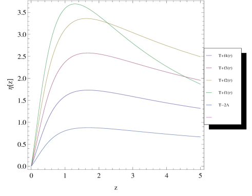
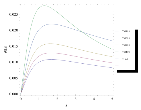
Figure 2: The graphs shows the deviation vector magnitude $\eta(z)$ (left panel) and observer area distance $r_{0}(z)$ (right panel) for null vector field GDE with FLRW background as functions of redshift. The graphs are plotted for $H_{0}=80Km/s/Mpc$, $\Omega_{m0}=0.3$, $\Omega_{r0}=\Omega_{k0}=0$, $\Lambda=1.7.10^{-121}$ and we imposed in equation (111) the initial conditions $\eta(z=0)=0$ and $\eta^{\prime}(z=0)=1$.

In each panel of Figure 2, we observe that the curves reflecting the evolution of the intensity of deviation vector $\eta(z)$ and the distance of the area of the observer $r_{0}(z)$ have similar behaviors to that of the model $\Lambda CDM$. Within the Model $f(T,\mathcal{T})=\gamma T^{\sigma}$, we see that when $\gamma$ is increasing ($\gamma\geqslant 1$) and we are going to larger values of redshift $(z\geqslant 0.8)$, the deviation vector intensity $\eta$ (z) and observer area distance $r_{0}(z)$ decouple from each model $\Lambda CDM$ but still keep the same pace while for small values of redshifts namely nowadays the model $f(T,\mathcal{T})$ can accurately replicate the model $\Lambda CDM$. We can then conclude that for all considered cases , the results are compactible to $\Lambda CDM$. So the above studied $f(T,\mathcal{T})$ models remain phenomenologically viable and can be tested with observational data.

V Conclusion

In this paper, we have presented the Geodesic Deviation Equation (GDE) in the context of $f(T,\mathcal{T})$ gravity applied to metric. The determination by rigorous calculation of the scalar Ricci and Riemann tensor was firstly executed by using the $f(T,\mathcal{T})$ gravity field equations. The Geodesic Deviation Equation and the generalization of Pirani equation for the FLRW Universe in $f(T,\mathcal{T})$ gravity have been investigated and both these equations have been reduced to the well known Mattig relation when $f(T,\mathcal{T})=-2\Lambda$. We have performed for two particular cases, the GDE for fundamental observes and the past-directed null vector fields with FLRW Universe. Within these cases we have obtained the Raychaudhuri equation, the generalized Mattig relation and the diametric angular distance differential for $f(T,\mathcal{T})$ gravity theory. Furthermore, as it is usually done in GR, we have also investigated the past-directed null geodesics condition for $f(T,\mathcal{T})$ gravity. Numerical results concerning the geodesic deviation $\eta(z)$ and the observer area distance $r_{0}(z)$ for $f(T,\mathcal{T})$ models were found and compared with their equivalent supplied by the $\Lambda CDM$ model.

References

• (1) C. W. Misner, K. S. Thorne, and J. H. Wheeler, Gravitation, W. H. Freeman and Company, 1973.
• (2) Szekeres P: The Gravitational Compass, J. Maths. Phys. 6 (1965), 1387.
• (3) J. L. Synge. On the Deviation of Geodesics and Null Geodesics, Particularly in Relation to the Properties of Spaces of Constant Curvature and Indefinite Line Element. Ann. Math. 35:705 (1934).
• (4) F. A. E. Pirani. On the Physical Significance of the Riemann Tensor. Acta Phys. Polon. 15:389 (1956).
• (5) G. F. R. Ellis and H. Van Elst. Deviation of geodesics in FLRW spacetime geometries (1997). Preprint in [arXiv:gr-qc/9709060v1].
• (6) S.L. Shapiro and S.A. Teukolsky, Black Holes, White Dwarfs and Neutron Satrs (Wile-Interscience, New York 1983).
• (7) K.S. Thorne, in S. Hawking and W. Israel, eds, 300 Year of Gravitation (Cambridge University, Cambridge 1987) p. 330.
• (8) Raychaudhuri A K: Relativistic Cosmology, Phys. Rev. 98 (1955), 1123.
• (9) Mattig W: Uber den Zusammenhang zwischen Rotverschiebung und scheinbarer Helligkeit, Astr. Nach. 284 (1958), 109.
• (10) Pirani F A E: On the Physical Significance of the Riemann Tensor, Acta Phys. Polon. 15 (1956),389.
• (11) D. N. Spergel, et. al., Astrophys. J. Suppl. 170, (2007) 377, arXiv:astro-ph/0603449.
• (12) J. K. Adelman-McCarthy, et. al., Astrophys. J. Suppl. 175, (2008) 297, arXiv:0707.3413[astro-ph].
• (13) R.Aldrovandi and J.G.Pereira,TELEPARALLEL GRAVITY,
in http://www.ift.unesp.br/users/jpereira/tele.pdf.
• (14) A. De Felice and S. Tsujikawa, Living Rel. Rev. 13, 3 (2010) [arXiv:1002.4928 [gr-qc]]; K. Bamba, S. Capozziello, S. Nojiri, S. D. Odintsov. Astrophys. Space Sci. 342, 155 (2012) [arXiv:1205.3421 [gr-qc]]; S. Nojiri and S. D. Odintsov, ECONF C 0602061, 06 (2006); Int. J. Geom. Meth. Mod. Phys. 4, 115-146 (2007) [arXiv:hep-th/0601213]; Phys. Rept. 505, 59-144 (2011) [arXiv:1011.0544].
• (15) T. Harko, F. S. N. Lobo, S. Nojiri and S. D. Odintsov, ?f(R, T ) gravity,? Phys. Rev. D 84 (2011) 024020. [arXiv:1104.2669 [gr-qc]].
• (16) M. J. S. Houndjo, Int. J. Mod. Phys. D. 21, 1250003 (2012). arXiv: 1107.3887 [astro-ph.CO].
• (17) M. J. S. Houndjo and O. F. Piattella, Int. J. Mod. Phys. D. 21, 1250024 (2012). arXiv: 1111.4275 [gr.qc].
• (18) D. Momeni, M. Jamil and R. Myrzakulov, Euro. Phys. J. C 72, arXiv: 1107.5807[physics.gen-ph].
• (19) M. J. S. Houndjo, C. E. M. Batista, J. P. Campos and O. F. Piattella,?? [arXiv:1203.6084 [gr-qc]].
• (20) F. G. Alvarenga, M. J. S. Houndjo, A. V. Monwanou and Jean. B. Chabi-Orou,?? arXiv: 1205.4678 [gr-qc].
• (21) S. ’i.Β Nojiri and S.Β D.Β Odintsov, β€œModified Gauss-Bonnet theory as gravitational alternative for dark energy,” Phys.Β Lett.Β B 631, 1 (2005) [hep-th/0508049]; S. Nojiri, S. D. Odintsov, A. Toporensky, P. Tretyakov, arXiv:0912.2488.
• (22) K. Bamba, S. D. Odintsov, L. Sebastiani, S. Zerbini, arXiv:0911.4390.
• (23) K. Bamba, C.-Q. Geng, S. Nojiri, S. D. Odintsov, arXiv:0909.4397.
• (24) M.E. Rodrigues, M.J.S. Houndjo, D. Momeni, R. Myrzakulov, arXiv:1212.4488.
• (25) M. J. S. Houndjo, M. E. Rodrigues, D. Momeni, R. Myrzakulov . arXiv:1301.4642 [gr-qc].
• (26) J.Β AmorΓ³s, J.Β de Haro and S.Β D.Β Odintsov, β€œBouncing Loop Quantum Cosmology from $f(T)$ gravity,” Physical Review D 87, 104037 (2013) [arXiv:1305.2344 [gr-qc]]; K.Β Bamba, J.Β de Haro and S.Β D.Β Odintsov, β€œFuture Singularities and Teleparallelism in Loop Quantum Cosmology,” JCAP 1302 (2013) 008 [arXiv:1211.2968 [gr-qc]]; K.Β Bamba, S. ’i.Β Nojiri and S.Β D.Β Odintsov, β€œEffective $f(T)$ gravity from the higher-dimensional Kaluza-Klein and Randall-Sundrum theories,” arXiv:1304.6191 [gr-qc]; G. R. Bengochea, R. Ferraro and , Phys. Rev. D 79, 124019 (2009) [arXiv:0812.1205 [astro-ph]].
• (27) E. V. Linder, Phys.Rev. D 81, 127301 (2010) [Erratum-ibid. D 82, 109902 (2010)] [arXiv:1005.3039 [astro-ph.CO]].
• (28) M. Jamil, D. Momeni and R. Myrzakulov, Eur. Phys. J. C 72 (2012) 2267 [arXiv:1212.6017 [gr-qc]].
• (29) R. Myrzakulov, Entropy 14 (2012) 1627[arXiv:1212.2155 [gr-qc]].
• (30) M. R. Setare and N. Mohammadipour, JCAP 1211 (2012) 030 [arXiv:1211.1375 [gr-qc]].
• (31) M.R. Setare, N. Mohammadipour, JCAP 01 (2013) 015 [arXiv: 1301.4891].
• (32) M. Jamil, D. Momeni, R. Myrzakulov and P. Rudra, J. Phys. Soc. Jap. 81 (2012) 114004 [arXiv:1211.0018 [physics.gen-ph]].
• (33) M. E. Rodrigues, M. J. S. Houndjo, D. Saez-Gomez and F. Rahaman, Phys. Rev. D 86 (2012) 104059 [arXiv:1209.4859 [gr-qc]].
• (34) M. Jamil, D. Momeni and R. Myrzakulov, Eur. Phys. J. C 72 (2012) 2122 [arXiv:1209.1298 [gr-qc]].
• (35) R. Myrzakulov, Eur. Phys. J. C 72 (2012)2203 [arXiv:1207.1039 [gr-qc]].
• (36) M. J. S. Houndjo, D. Momeni and R. Myrzakulov, Int. J. Mod. Phys. D 21 (2012) 1250093 [arXiv:1206.3938 [physics.gen-ph]].
• (37) M. E. Rodrigues, M. H. Daouda and M. J. S. Houndjo, arXiv:1205.0565 [gr-qc].
• (38) M. R. Setare and M. J. S. Houndjo, arXiv:1203.1315 [gr-qc].
• (39) K. Bamba, M. Jamil, D. Momeni and R. Myrzakulov, arXiv:1202.6114 [physics.gen-ph].
• (40) K. Bamba, R. Myrzakulov, S. ’i. Nojiri and S. D. Odintsov, Phys. Rev. D 85 (2012)104036 [arXiv:1202.4057 [gr-qc]].
• (41) M. Jamil, D. Momeni and R. Myrzakulov, Eur. Phys. J. C 72 (2012) 2267 [arXiv:1212.6017[gr-qc]].
• (42) M. Jamil, D. Momeni and R. Myrzakulov, Gen. Rel. Grav. 45 (2013) 263 [arXiv:1211.3740 [physics.gen-ph]].
• (43) M. Jamil, D. Momeni and R. Myrzakulov, Eur. Phys. J. C 72 (2012) 2122 [arXiv:1209.1298 [gr-qc]].
• (44) M. Jamil, D. Momeni and R. Myrzakulov, Eur. Phys. J. C 72 (2012) 2075 [arXiv:1208.0025 [gr-qc]].
• (45) M. Jamil, K. Yesmakhanova, D. Momeni and R. Myrzakulov, Central Eur. J. Phys. 10 (2012) 1065 [arXiv:1207.2735 [gr-qc]].
• (46) M. J. S. Houndjo, D. Momeni and R. Myrzakulov, Int. J. Mod. Phys. D 21 (2012) 1250093 [arXiv:1206.3938 [physics.gen-ph]].
• (47) M. Jamil, D. Momeni and R. Myrzakulov, Eur. Phys. J. C 72 (2012) 1959 [arXiv:1202.4926 [physics.gen-ph]].
• (48) M. H. Daouda, M. E. Rodrigues and M. J. S. Houndjo, Phys. Lett. B 715 (2012) 241 [arXiv:1202.1147 [gr-qc]].
• (49) M. Jamil, S. Ali, D. Momeni, R. Myrzakulov and Eur. Phys. J. C 72, 1998 (2012) [arXiv:1201.0895 [physics.gen-ph]].
• (50) M. Jamil, D. Momeni, N. S. Serikbayev, R. Myrzakulov and , Astrophys. Space Sci. 339, 37 (2012) [arXiv:1112.4472 [physics.gen-ph]].
• (51) M. Jamil, D. Momeni, M. A. Rashid and , Eur. Phys. J. C 71, 1711 (2011) [arXiv:1107.1558 [physics.gen-ph]].
• (52) M. Hamani Daouda, M. E. Rodrigues and M. J. S. Houndjo, Eur. Phys. J. C 72 (2012) 1893 [arXiv:1111.6575 [gr-qc]].
• (53) M. Hamani Daouda, M. E. Rodrigues and M. J. S. Houndjo, Eur. Phys. J. C 72 (2012) 1890 [arXiv:1109.0528 [physics.gen-ph]].
• (54) R. Myrzakulov, Gen. Rel. Grav. 44 (2012) 3059 [arXiv:1008.4486 [physics.gen-ph]].
• (55) K. K. Yerzhanov, S. .R. Myrzakul, I. I. Kulnazarov and R. Myrzakulov, arXiv:1006.3879 [gr-qc].
• (56) R. Myrzakulov, Eur. Phys. J. C 71 (2011) 1752 [arXiv:1006.1120 [gr-qc]].
• (57) M. E. Rodrigues, M. J. S. Houndjo, D. Momeni, R. Myrzakulov and , arXiv:1302.4372 [physics.gen-ph].
• (58) J. M. Bardeen, B. Carter, S. W. Hawking , Commun. Math. Phys. 31 (1973) 161-170.
• (59) N. Tamanini and C. G. Boehmer, Phys. Rev. D 86, 044009 (2012), arXiv:1204.4593 [gr-qc].
• (60) Baojiu Li, T. P. Sotiriou and J. D. Barrow, Phys. Rev. D 83, 064035 (2011); Phys. Rev. D 83, 104030 (2011).
• (61) M. J. S. Houndjo, D. Momeni, R. Myrzakulov and M. E. Rodrigues,arXiv:1304.1147.
• (62) C. Deliduman and B. Yapiskan, arXiv:1103.2225v3 [gr-qc].
• (63) M. Hamani Daouda, M. E. Rodrigues and M. J. S. Houndjo, Eur. Phys. J. C 71 (2011) 1817 [arXiv:1108.2920 [astro-ph.CO]].
• (64) I.G.Salako, M.E.Rodrigues, A.V.Kpadonou, M. J.S.Houndjo and J.Tossa JCAP 060, 1475-7516 (2013)
• (65) M. E. Rodrigues, I. G. Salako, M. J. S. Houndjo, J. Tossa Int. J. Mod. Phys. D 23, 1450004 (2014)
• (66) Davood Momeni, Ratbay Myrzakulov.: arXiv:1405.5863 [gr-qc]
• (67) Tiberiu Harko, Francisco S. N. Lobo, G. Otalora,and Emmanuel N. Saridakis http://arxiv.org/abs/1405.0519v1
• (68) Ines G. Salako, Abdul Jawad, Surajit Chattopadhyay, Astrophys.Space Sci. 358 (2015) 1, 13
• (69) S. B. Nassur, M. J. S. Houndjo, A. V. Kpadonou, M. E. Rodrigues, J. Tossa, http://arxiv.org/abs/1506.09161
• (70) R. Ferraro and F. Fiorini, Phys. Rev. D 75 (2007) 084031
• (71) G. R. Bengochea and R. Ferraro, Phys. Rev. D 79(2009)124019
• (72) A. Guarnizo, L. Castaneda, J. M. Tejeiro, Gen. Rel. Grav. 43, 2713 (2011); A. de la Cruz-Dombriz, P. K. S. Dunsby, V. C. Busti, S. Kandhai, Phys. Rev. D 89, 064029 (2014), arXiv:1312.2022; A. Guarnizo, L. Castaneda, J. M. Tejeiro, arXiv:1402.3196.
• (73) F. Shojai and A. Shojai, Phys. Rev. D 78, 104011 (2008).
• (74) F. Darabi, M. Mousavi, K. Atazadeh, Dec 31, 2014. 11 pp. Published in Phys.Rev. D91 (2015) 084023.
• (75) E. H. Baffou, M. J. S. Houndjo, M. E. Rodrigues, A. V. Kpadonou, J. Tossa, arXiv:1509.06997
• (76) R. M. Wald, General Relativity, The University of Chicago Press, 1984;
E. Poisson, A Relativist’s Toolkit - The Mathematics of Black-Hole Mechanics, Cambridge University Press, 2004.
• (77) J. L. Synge, Ann. Math. 35, 705 (1934);
F. A. E. Pirani, Acta Phys. Polon. 15, 389 (1956);
G. F. R. Ellis and H. Van Elst, [arXiv:gr-qc/9709060v1].
• (78) G. F. R. Ellis and H. Van Elst, [arXiv:gr-qc/9812046v5].
• (79) D. L. Caceres, L. CastaΒ neda, J. M. Tejeiro, J. Phys. Conf. Ser. 229, 012076 (2010), [arXiv:0912.4220v1].
• (80) G.R. Bengochea and R. Ferraro, Phys. Rev. D 79, 124019 (2009), [arXiv:0812.1205].
• (81) P. Schneider, J. Ehlers and E. E. Falco, Gravitational Lenses, (Springer-Verlag, 1999).
• (82) Ines.G.Salako, M. J. S. Houndjo, M. E. Rodrigues, and A. V. Kpadonou, to Appear