Topological Anderson Insulators in Systems without Time-Reversal Symmetry

Abstract

Occurrence of topological Anderson insulator (TAI) in HgTe quantum well suggests that when time-reversal symmetry (TRS) is maintained, the pertinent topological phase transition, marked by re-entrant $2e^{2}/h$ quantized conductance contributed by helical edge states, is driven by disorder. Here we show that when TRS is broken, the physics of TAI becomes even richer. The pattern of longitudinal conductance and nonequilibrium local current distribution displays novel TAI phases characterized by nonzero Chern numbers, indicating the occurrence of multiple chiral edge modes. Tuning either disorder or Fermi energy (in both topologically trivial and nontrivial phases), drives transitions between these distinct TAI phases, characterized by jumps of the quantized conductance from $0$ to $e^{2}/h$ and from $e^{2}/h$ to $2e^{2}/h$. An effective medium theory based on the Born approximation yields an accurate description of different TAI phases in parameter space.

I Introduction

The quest for understanding novel electronic properties of topological insulators (TIs) stirred intense experimental and theoretical studies [1, 2, 3, 4, 5, 6, 7, 8, 9]. Observations of quantized conductance at $2e^{2}/h$ in time reversal invariant TIs [4, 5] and at $e^{2}/h$ in magnetically doped TIs [9] confirm the occurrence of the quantum spin Hall (QSH) and the quantum anomalous Hall (QAH) effects. A well accepted paradigm is that the main distinction of TIs from trivial insulators is the existence of topologically protected gapless edge states that conduct (either charge or spin) even at strong disorder [10, 11]. Recently, a novel family of TIs whose helical edge states can be induced by disorder was discovered [12, 13, 14, 15, 16, 17, 18, 19, 20, 21, 22, 23]. Explicitly, as disorder strength increases from zero, the conductance initially decreases, but then, within a certain region of disorder, it is quantized at $2e^{2}/h$ before dropping to zero at stronger disorder [12, 13, 14, 15, 16, 17, 18, 19, 20, 21, 22, 23]. This (evidently nontrivial) phase of matter is termed as topological Anderson insulator (TAI). Specifically, disorder drives topological phase (TP) transitions by modifying the topological mass and chemical potential of HgTe quantum well [14]. Interestingly, TAI in three dimensions has also been identified in a cubic lattice in which electrons are subject to strong spin-orbit coupling (SOC) [15].

So far, TAI was studied mainly in systems that maintain time-reversal symmetry (TRS) for which the Chern number vanishes and edge states are helical. In this work we suggest a model for exposing the (even richer) physics of TAI in systems with broken TRS. As we show, these systems support multiple chiral edge states, and display novel TAI phases characterized by nonzero Chern numbers. Even in the absence of disorder, the model exhibits nontrivial TPs including the QAH phases with Chern numbers $C=\pm 1$ and $\pm 2$, and the TRS-broken QSH phase whose helical edge states are not topologically protected [24]. Then, adding on-site disorder (of strength $W$), the TAI phases are identified by re-entrant $e^{2}/h$ and $2e^{2}/h$ quantized conductance plateaus. By using a combination of numerical methods and an effective medium theory based on the Born approximation [14], the Chern number and bulk band gap evolution are evaluated in the $W-E_{F}$ plane. Inspection of the nonequilibrium local current distribution (NLCD) in the nontrivial TAI phases further confirms the conjecture that quantized conductance plateaus are due to chiral edge states and that transitions between these plateaus are drivable by tuning either disorder or Fermi energy.

II Model

In order to study TAI in magnetic systems that lift spin degeneracy and break TRS, we consider electrons hopping on a hexagonal lattice subject to SOC, staggered sublattice potential, antiferromagnetic exchange field [25, 26, 27, 28], and off-resonant circularly polarized light [29, 30, 31]. The tight-binding Hamiltonian reads

$$\begin{split}H=&t\sum_{\langle ij\rangle}c_{i}^{\dagger}c_{j}+\lambda_{v}\sum_{i}\mu_{i}c_{i}^{\dagger}c_{i}+\sum_{i}\epsilon_{i}c_{i}^{\dagger}c_{i}\\ &+i\lambda_{so}\sum_{\langle\langle ij\rangle\rangle}\nu_{ij}c_{i}^{\dagger}s^{z}c_{j}+i\lambda_{r}\sum_{\langle ij\rangle}c_{i}^{\dagger}(\bm{s}\times\hat{\bm{d}}_{ij})_{z}c_{j}\\ &+\lambda_{am}\sum_{i}\mu_{i}c_{i}^{\dagger}s^{z}c_{i}+i\lambda_{l}\sum_{\langle\langle ij\rangle\rangle}\nu_{ij}c_{i}^{\dagger}c_{j}.\end{split}$$ (1)

The various symbols in Eq. (1) are defined as follows: $i$ and $j$ label the lattice sites, while $\langle ij\rangle$ and $\langle\langle ij\rangle\rangle$ stand for nearest neighbor (NN) and next nearest neighbor (NNN) sites. $\bm{s}=(s^{x},s^{y},s^{z})$ is the vector of Pauli matrices acting in spin space. $\nu_{ij}=(2/\sqrt{3})(\hat{\bm{d}}_{1}\times\hat{\bm{d}}_{2})_{z}=\pm 1$ is defined by lattice geometry where $\hat{\bm{d}}_{1}$ and $\hat{\bm{d}}_{2}$ are two unit vectors along NN bonds connecting site $i$ to its NNN site $j$, $\hat{\bm{d}}_{ij}$ is a unit vector connecting two NN sites $i$ and $j$, and $\mu_{i}=\pm 1$ denotes A and B sublattices. The first two terms describe NN hopping and staggered sublattice potential with respective strengths $t$ and $\lambda_{v}$. The third term represents on-site disorder in which $\{\epsilon_{i}\in[-W/2,W/2]\}$ are i.i.d. The fourth and fifth terms describe the intrinsic and Rashba SOC with respective strengths $\lambda_{so}$ and $\lambda_{r}$. The first five terms respect TRS, and can be viewed as a disordered version of the Kane-Mele model [1]. The last two terms break TRS, and are termed as the antiferromagnetic exchange field [25, 26, 27, 28] and off-resonant circularly polarized light [29, 30, 31] with strengths $\lambda_{am}$ and $\lambda_{l}$. The last term is named so because it is originally derived from the interaction of electrons with a vertically incident weak circularly polarized light of high frequency ($\gg t/\hbar$). Such that the off-resonant conditions are satisfied and high order effects can be neglected [29, 30, 31]. By using the Floquet theory [32, 33], the time-dependent problem is transformed to a static problem encoded in the effective Hamiltonian described by the last term in Eq. (1) [29, 30, 31]. Of course, this term may be generated by other means such as by staggered magnetic flux in the Haldane model [34].

III Clean case: Topological phases

In the absence of disorder, this model supports the QAH phases with $C=\pm 1$ and $\pm 2$. The Hamiltonian Eq. (1) is block-diagonized in momentum space as $H=\sum_{\bm{k}}c_{\bm{k}}^{\dagger}\mathcal{H}(\bm{k})c_{\bm{k}}$. In the basis of $\{|\text{A},\uparrow\rangle,|\text{A},\downarrow\rangle,|\text{B},\uparrow\rangle,|\text{B},\downarrow\rangle\}$, $\mathcal{H}(\bm{k})$ can be expressed in terms of the Dirac $\Gamma$ matrices [35] as

$$\mathcal{H}(\bm{k})=d_{0}(\bm{k})\text{I}^{4}+\sum_{a=1}^{5}d_{a}(\bm{k})\Gamma^{a}+\sum_{a<b=1}^{5}d_{ab}(\bm{k})\Gamma^{ab},$$ (2)

where $\text{I}^{4}$ is the $4\times 4$ identity matrix and the nonvanishing $d_{a}$ and $d_{ab}$ factors are shown in Ref. [36]. To be concrete (and without loss of generality), $\lambda_{r}=\lambda_{am}=0.3t$ and $\lambda_{so}$=$0.2t$ are fixed below while $(\lambda_{l},\lambda_{v})$ are tunable parameters to realize various TPs (identified by their corresponding Chern numbers). TP transitions occur at the closure and reopening of the bulk band gap. For $\mathcal{H}(\bm{k})$, gap closure and reopening occurs (at $K$ and $K^{\prime}$ valley) whenever,

$$2\left|f_{\eta}\right|-\left|\lambda_{\eta}\right|=\sqrt{\lambda_{\eta}^{2}+9\lambda_{r}^{2}},$$ (3)

where $f_{\eta}=\lambda_{am}-3\sqrt{3}\eta\lambda_{so}$ and $\lambda_{\eta}=\lambda_{v}-3\sqrt{3}\eta\lambda_{l}$, while $\eta=\pm 1$ denotes $K$ and $K^{\prime}$ valley, respectively. At half filling, the Chern number is calculated for the valence bands in the $\lambda_{l}/\lambda_{so}-\lambda_{v}/\lambda_{so}$ plane based on the numerical method developed in Ref.  [37]. The results are shown in Fig. 1(a) where TPs are classified by different colors and the Chern numbers. The TP boundaries of Eq. (3) (red solid and blue dash lines) separate different TPs as shown in Fig. 1(a). Crossing points of two different phase boundary lines correspond to simultaneous closure of the bulk band gap at two different valleys. These are verified by the band structures (Fig. 1(b)-(d)) at three points marked as b, c, d on the TP boundaries as shown in Fig. 1(a).

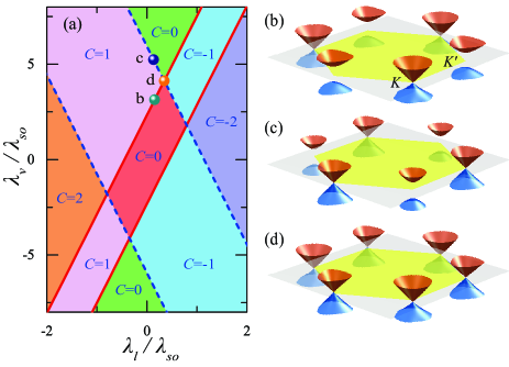
Figure 1: (color online) (a) Phase diagram in the $\lambda_{l}/\lambda_{so}-\lambda_{v}/\lambda_{so}$ plane. Red solid and blue dash lines are the TP boundaries at which the bulk band gap closes at $K$ and $K^{\prime}$ valleys respectively. Various TPs with different colors are specified by the Chern number $C$. The $C=0$ phases are further distinguished by a pair of spin Chern numbers as $(C_{+},C_{-})=(0,0)$ marked by green and $(\pm 1,\mp 1)$ marked by red. The low-energy band structures near the $K$ and $K^{\prime}$ valleys (corresponding to the three TP boundary points labeled as b, c, and d in (a)) are shown in (b), (c), and (d).

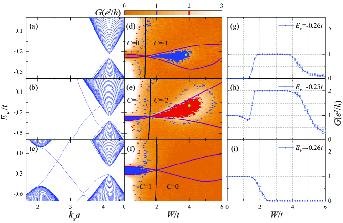
Figure 2: (color online) (a)-(c): Low-energy band structures of the nanoribbons with zigzag edges in the trivial, QAH1, and QAH2 phases whose parameters are specified in the text. (d)-(f): Density plot of longitudinal conductance of the nanoribbons corresponding to (a)-(c). The black and purple lines are respective TP boundary and bulk band gap evolution predicted by the Born approximation in the $W-E_{F}$ plane. The colorbar is terminated at $G=3$ and $G\geq 3$ is represented by white. (g)-(i): Conductance profiles are displayed as a function of disorder strength for given Fermi energies within the bulk band gap.

Two distinct $C=0$ phases exist with different spin Chern numbers $(C_{+},C_{-})$ defined in Ref. [38, 39]: The first, $(C_{+},C_{-})$=$(0,0)$ (green color region in Fig. 1(a)) is a topologically trivial insulator. The second, $(C_{+},C_{-})=(\pm 1,\mp 1)$ (red color region in Fig. 1(a)) is the QSH insulator (strictly protected only if TRS is respected). When TRS is broken two counter-propagating chiral edge states could annihilate each other. Nevertheless, when the TRS is only weakly broken, the edge states that suffer from the backward scattering can still exist, and capable of transporting charge and spin although not in a perfect (quantized) value [24]. In other words, the edge states are not topologically protected, and, at strong disorder, they will be destroyed [40].

In order to elucidate the role of edge states, we consider the model on a long strip with zigzag edges. The energy spectrum of $\mathcal{H}(\bm{k})$ is evaluated numerically for $(\lambda_{l},\lambda_{v})=(0.25t,1.8t)$ in the trivial phase, $(0.35t,1.4t)$ in the QAH1 phase with $C=-1$, and $(0.03t,0.7t)$ in the QAH2 phase with $C=1$. The corresponding band structures are shown in Fig. 2(a)-(c). The edge modes are clearly visible for the QAH1 and QAH2 phases.

IV TAI: Broken TRS and role of disorder

To study TAI phases within this model, we elucidate the effect of on-site disorder on the longitudinal conductance in a two-terminal setup: A long strip of size $200a/\sqrt{3}\times 1000a$ is connected to two semi-infinite leads at the two ends. Here $a$ is the in-plane lattice constant. Existence or absence of edge channels due to disorder in different phases can be clearly seen from the density plot of longitudinal conductance (averaged over 5 disorder realizations) in the $W-E_{F}$ plane as shown in Fig. 2(d)-(f). In the trivial phase, as disorder increases, a $e^{2}/h$ quantized conductance plateau appears in the bulk band gap as shown in Fig. 2(d). In the QAH1 phase, as expected, $e^{2}/h$ quantized conductance plateau exists within the bulk band gap. However, it shoots up to $2e^{2}/h$ above a critical disorder and penetrates into the conduction band as disorder increases further (see Fig. 2(e)). In the QAH2 phase, the $e^{2}/h$ quantized conductance plateau is terminated at relatively weak disorder as shown in Fig. 2(f). The corresponding conductance profiles as a function of disorder strength for given Fermi energies within the bulk band gap are respectively shown in Fig. 2(g)-(i). The data is obtained by averaging over 100 realizations. The absence of fluctuation within the quantized conductance plateaus indicates that they are contributed by topologically protected edge states.

To corroborate this physical interpretation, we analyze the present model within an effective medium theory based on the Born approximation in which high order scattering processes are neglected [14]. In this formalism, the role of disorder is encoded in the self-energy,

$$\begin{split}\Sigma(W,E_{F})&=\frac{W^{2}}{12S_{\text{BZ}}}\int_{\text{BZ}}d^{2}\textbf{{k}}\left[E_{F}+i0^{+}-\mathcal{H}(\textbf{{k}})\right]^{-1}.\end{split}$$ (4)

Here $S_{\text{BZ}}$ is the area of the first Brillouin zone and $\mathcal{H}(\bm{k})$ is the $4\times 4$ Hamiltonian given in Eq. (2). The self-energy can also be decomposed into the summation of the Dirac $\Gamma$ matrices. Thus, the effective Hamiltonian in the presence of disorder is

$$\overline{\mathcal{H}}(\bm{k},W,E_{F})=\mathcal{\mathcal{H}}(\bm{k})+\Sigma(W,E_{F}).$$ (5)

Due to the violation of time-reversal, spin rotation, inversion, and particle-hole symmetries, $\Sigma(W,E_{F})$ is a full $4\times 4$ matrix (for $W\neq 0$) that modifies the parameters of $\mathcal{H}(\bm{k})$ and shifts the Dirac points away from the $K$ and $K^{\prime}$ valley.

To demonstrate the disorder-induced TP transitions, the Chern number $C(W,E_{F})$ of the effective Hamiltonian $\overline{\mathcal{H}}(\bm{k},W,E_{F})$ is evaluated for various $W$ and $E_{F}$ by using the same method mentioned early for $\mathcal{H}(\bm{k})$. The results are shown in Fig. 2(d)-(f) where the TP boundaries are marked by black solid lines and different TPs are specified by Chern numbers. The disorder-induced TP transitions are: (i) trivial phase $(C=0)$ $\rightarrow$ QAH phase $(C=-1)$; (ii) QAH phase $(C=-1)$ $\rightarrow$ QAH phase $(C=-2)$; (iii) QAH phase $(C=1)$ $\rightarrow$ TRS-broken QSH phase $(C=0)$. In order to further determine the TAI phases in the $W-E_{F}$ plane, the bulk band gap evolution under disorder is evaluated and is represented by purple lines in Fig. 2(d)-(f). (Recall that the appearance of edge states requires the Fermi energy to lie in the bulk band gap). Indeed, band inversion occurs at the TP boundary. Thus, for modest disorder, this effective medium theory yields an adequate description of the various TAI phases in the $W-E_{F}$ plane. The peculiarity of these TAI phases is that they are characterized by nonzero Chern numbers as a result of broken TRS. In analogy with the distinction between QAH and QSH phases, the TAI phases found in systems without TRS are distinct from the one studied previously in systems that respect TRS.

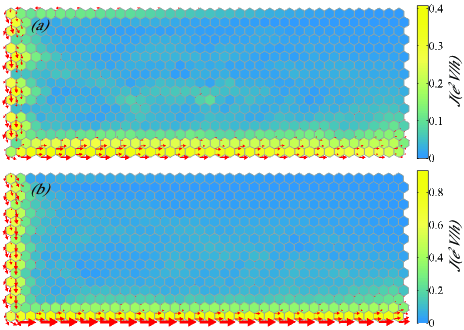
Figure 3: (color online) The averaged NLCD in nanoribbons for different TAI phases and with various disorder strengths $W$ and Fermi energies $E_{F}$ in a two-terminal setup. The color in each hexagon is the average value of the NLCs at six corners. The red arrows denote current direction at each lattice site. The arrow size is proportional to the magnitude of NLC. $eV$ denotes the chemical potential difference between the source and drain. (a) $W=3.8t$ and $E_{F}=-0.25t$ (marked by green spot in Fig. 2(d)). (b) $W=4t$ and $E_{F}=-0.1t$ (marked by green spot in Fig. 2(e)).

V Nonequilibrium local current distribution (NLCD)

To further substantiate the assertion that the re-entrant quantized conductance plateaus in Fig. 2(d) and (e) originate from the robust chiral edge states, we study the NLCD (averaged over 1000 ensembles). In the two-terminal setup specified above, the strip size is set as $26a/\sqrt{3}\times 40a$ here. Consider first the disorder induced $e^{2}/h$ quantized conductance plateau shown in Fig. 2(d). For $(W,E_{F})=(3.8t,-0.25t)$ (green dot in Fig. 2(d)) that is in the $C=-1$ TAI phase, the NLCD is shown in Fig. 3(a). Apparently, the nonequilibrium local currents (NLCs) are strongly localized at the bottom edge. The NLCs at the top edge are suppressed because the charge motion is directed against the source-drain bias voltage. Similar NLCD is found in the $2e^{2}/h$ quantized conductance plateau. For $(W,E_{F})=(4t,-0.1t)$ (marked by green spot in Fig. 2(e)) within the $C=-2$ TAI phase, the NLCD is shown in Fig. 3(b). As expected, the edge current is roughly twice higher than that encountered in Fig. 3(a) since the Chern number is doubled. Namely, the number of edge channels is doubled. The fact that the two edge modes propagate in the same direction at the same edge indicates that the edge states are chiral, not helical. Thus, our results pertaining the NLCD are consistent with the conclusions obtained within the Born approximation.

VI Discussion

So far, the TAI was observed and analyzed in systems that respect TRS. In these systems, the Chern number is strictly zero. Thus only trivial and QSH phases can exist, and there are either zero or two Kramer degenerate helical edge channels. Consequently, the conductance can only jump from $0$ to $2e^{2}/h$ or vice versa. It was not clear from previous studies how the topologically protected edge channels are created and destroyed by disorder in systems without TRS, where the TAI phases can have nonzero Chern numbers and support chiral edge states. In fact, the appearance of robust multiple chiral edge modes in our model is striking and nontrivial within our current understanding of TAI [11]. The present work shows the edge channels can be created and/or destroyed one-by-one, resulting in multiple quantized conductance plateaus. Furthermore, previous works can only be realized in non-magnetic materials. Our model could be realized in magnetic materials. As for the experimental detection, the TAI in systems without TRS can support both even and odd numbers quantized conductance plateaus in units of $e^{2}/h$. However, only even number quantized conductance is permitted in TAI with TRS studied previously. For QSH states in the present case where the TRS is broken, helical edge states are not topologically protected as expected. However, these edge states, suffering the backward scattering, can still exist at weak disorder and transport charge and spin [24, 40].

VII Summary

We present a tight-binding model on a hexagonal lattice that breaks both time-reversal and spin rotation symmetries. It displays several TPs, including the QAH phases with $C=\pm 1$ and $C=\pm 2$, as well as the TRS-broken QSH phase. In the presence of on-site disorder, the longitudinal conductance within various TPs is displayed in the $W-E_{F}$ plane and exposes new TAI phases. They are characterized by nonzero Chern numbers, and can be experimentally identified from the re-entrant $e^{2}/h$ and $2e^{2}/h$ quantized conductance plateaus. Disorder-induced TP transitions are marked by jumps of the quantized conductance from 0 to $e^{2}/h$ and from $e^{2}/h$ to $2e^{2}/h$. An effective medium theory based on the Born approximation adequately encodes all transitions among these TAI phases. Analysis of the NLCD further confirms the interpretation that quantized conductance plateaus originate from chiral edge states, similar to the QAH and quantum Hall effects.

VIII Acknowledgment

This work is supported by NSFC of China grant (11374249) and Hong Kong RGC grants (163011151 and 605413). The research of Y.A is partially supported by Israeli Science Foundation grant 400/2012.

References

- [1] C. L. Kane and E. J. Mele, Phys. Rev. Lett. 95, 146802 (2005).
- [2] C. L. Kane and E. J. Mele, Phys. Rev. Lett. 95, 226801 (2005).
- [3] B. A. Bernevig, T. L. Hughes, and S. C. Zhang, Science 314, 1757 (2006).
- [4] M. König, S. Wiedmann, C. Brüne, A. Roth, H. Buhmann, L. W. Molenkamp, X. L. Qi, and S. C. Zhang, Science 318, 766 (2007).
- [5] A. Roth, C. Brüne, H. Buhmann, L. W. Molenkamp, J. Maciejko, X. L. Qi, and S. C. Zhang, Science 325, 294 (2009).
- [6] M. Z. Hasan and C. L. Kane, Rev. Mod. Phys. 82, 3045, (2010).
- [7] J. E. Moore, Nature 464, 194 (2010).
- [8] X. L. Qi and S. C. Zhang, Rev. Mod. Phys. 83, 1057 (2011).
- [9] C. Z. Chang, J. Zhang, X. Feng, J. Shen, Z. Zhang, M. Guo, K. Li, Y. Ou, P. Wei, L. L. Wang, Z. Q. Ji, Y. Feng, S. Ji, X. Chen, J. Jia, X. Dai, Z. Fang, S. C. Zhang, K. He, Y. Wang, L. Lu, X. C. Ma, and Q. K. Xue, Science 340, 167 (2013).
- [10] L. Sheng, D. N. Sheng, C. S. Ting, and F. D. M. Haldane, Phys. Rev. Lett. 95, 136602 (2005).
- [11] I. C. Fulga, B. van Heck, J. M. Edge, and A. R. Akhmerov, Phys. Rev. B 89, 155424 (2014).
- [12] J. Li, R. L. Chu, J. K. Jain, and S. Q. Shen, Phys. Rev. Lett. 102, 136806 (2009).
- [13] H. Jiang, L. Wang, Q. F. Sun, and X. C. Xie, Phys. Rev. B 80, 165316 (2009).
- [14] C. W. Groth, M. Wimmer, A. R. Akhmerov, J. Tworzyd lo, and C. W. J. Beenakker, Phys. Rev. Lett. 103, 196805 (2009).
- [15] H. M. Guo, G. Rosenberg, G. Refael, and M. Franz, Phys. Rev. Lett. 105, 216601 (2010).
- [16] W. Li, J. D. Zang, and Y. J. Jiang, Phys. Rev. B 84, 033409 (2011).
- [17] Y. X. Xing, L. Zhang, and J. Wang, Phys. Rev. B 84, 035110 (2011).
- [18] Y. Y. Zhang, R. L. Chu, F. C. Zhang, and S. Q. Shen, Phys. Rev. B 85, 035107 (2012).
- [19] J. Song, H. Liu, H. Jiang, Q. F. Sun, and X. C. Xie, Phys. Rev. B 85, 195125 (2012).
- [20] D. Xu, J. Qi, J. Liu, Sacksteder V., X. C. Xie, and H. Jiang, Phys. Rev. B 85, 195140 (2012).
- [21] Y. Y. Zhang and S. Q. Shen, Phys. Rev. B 88, 195145 (2013).
- [22] A. Girschik, F. Libisch, and S. Rotter, Phys. Rev. B 91, 214204 (2015).
- [23] C. P. Orth, T. Sekera, C. Bruder, and T. L. Schmidt, Sci. Rep. 6, 24007 (2016).
- [24] Y. Yang, Z. Xu, L. Sheng, B. Wang, D. Y. Xing, and D. N. Sheng, Phys. Rev. Lett. 107, 066602 (2011).
- [25] X. Li, T. Cao, Q. Niu, J. Shi, and J. Feng, Proc. Natl Acad. Sci. USA 110, 3738 (2013).
- [26] M. Ezawa, Phys. Rev. B 87, 155415 (2013).
- [27] Q. F. Liang, L. H. Wu, and X. Hu, New J. Phys. 15, 063031 (2013).
- [28] M. Ezawa, Phys. Rev. Lett. 114, 056403 (2015).
- [29] J. I. Inoue and A. Tanaka, Phys. Rev. Lett. 105, 017401 (2010).
- [30] T. Kitagawa, T. Oka, A. Brataas, L. Fu, and E. Demler, Phys. Rev. B 84, 235108 (2011).
- [31] M. Ezawa, Phys. Rev. Lett. 110, 026603 (2013).
- [32] J. H. Shirley, Phys. Rev. 138, B979 (1965).
- [33] H. Sambe, Phys. Rev. A 7, 2203 (1973).
- [34] F. D. M. Haldane, Phys. Rev. Lett. 61, 2015 (1988).
- [35] The Dirac matrices are defined as: and [1], where and are Pauli matrices acting in sublattice and spin spaces.
- [36] The nonvanishing and factors in Eq. (2) are: , , , , , , , , where and .
- [37] T. Fukui, Y. Hatsugai, and H. Suzuki, J. Phys. Soc. Jpn. 74, 1674 (2005).
- [38] D. N. Sheng, Z. Y. Weng, L. Sheng, and F. D. M. Haldane, Phys. Rev. Lett. 97, 036808 (2006).
- [39] E. Prodan, Phys. Rev. B 80, 125327 (2009).
- [40] See supplemental material.